Data Compression for Proof Replay

J Autom Reasoning (2008) 41:193–218DOI 10.1007/s10817-008-9109-2

Data Compression for Proof Replay

Hasan Amjad

Received: 14 November 2008 / Accepted: 14 November 2008 / Published online: 9 December 2008© Springer Science + Business Media B.V. 2008

Abstract We describe a compressing translation from SAT solver generated propo-sitional resolution refutation proofs to classical natural deduction proofs. The re-sulting proof can usually be checked quicker than one that simply simulates theoriginal resolution proof. We use this result in interactive theorem provers, to speedup reconstruction of SAT solver generated proofs. The translation is fast and scalesup to large proofs with millions of inferences.

Keywords Proof translation · SAT solvers · Interactive theorem proving

1 Introduction

Interactive theorem provers like Coq [18], PVS [23], HOL4 [11], Isabelle [24] andHOL Light [15] traditionally support rich specification logics. Automation for theselogics is limited in theory and hard in practice, and proving a non-trivial theoremusually requires manual guidance by an expert user. Automatic proof procedures onthe other hand, while designed for simpler logics, have become increasingly powerfulover the past few years. By integrating automated procedures with interactivesystems, we can preserve the richness of our specification logic and at the same timeincrease the degree of proof automation for useful fragments of that logic [25].

Formal verification is an important application area of interactive theorem prov-ing. Problems in verification can often be reduced to Boolean satisfiability (SAT)[2–4] and so the performance of an interactive prover on propositional problemsmay be of significant practical importance. SAT solvers [8, 22] are powerful proofprocedures for propositional logic and it is natural to wish to use them as proofengines for interactive provers.

H. Amjad (B)University of Cambridge Computer Laboratory, William Gates Building,15 JJ Thomson Avenue, Cambridge CB3 0FD, UKe-mail: [email protected]

194 H. Amjad

There are many approaches to such an integration. The pragmatic approach is totrust the result of the SAT solver and assert it as a theorem in the prover. The dangeris that of soundness bugs in the solver but more likely in the relatively untestedinterface code, which may involve complex translations to propositional logic. Thesafest approach would be to execute the SAT solver algorithm within the prover, butwe reject this on the grounds of efficiency. A good middle ground is to verify the SATsolver proof, and this is the approach we take. The extra assurance of soundness isparticularly suited for those industrial applications where the focus is on certificationrather than debugging.

Recent work [9, 28] showed how interactive provers could use SAT solvers asnon-trusted decision procedures for propositional logic, by simulating propositionalresolution in their proof systems. We now show how to translate the resolution proofto a natural deduction proof that can be replayed faster than a natural deductionproof that directly simulates the resolution proof. The idea is to memoise parts ofthe proof by adapting standard data compression techniques. The treatment is toolindependent, and assumes only that the interactive prover supports propositionallogic and can simulate classical natural deduction.

The next section gives all the background required to keep the paper reasonablyself-contained. In Sections 3 and 4, we look at proof reconstruction and memoisationrespectively. Finally, we give experimental results in Section 5.

2 Preliminaries

2.1 SAT Solver Proof Structure

We restrict ourselves to proofs produced by conflict driven clause learning SATsolvers based on the DPLL algorithm [6]. The presentation here is based on a tutorialintroduction by Mitchell [20]. A SAT solver takes as input a term in conjunctivenormal form (CNF), a conjunction of disjunctions of literals. A literal is a possiblynegated atomic proposition. The negation of an atomic proposition p is denoted byp. Each disjunct term of the conjunction is called a clause. Since both conjunction anddisjunction are associative, commutative and idempotent, clauses can also be thoughtof as sets of literals, and the entire formula as a set of clauses. A unit clause is oneconsisting of a single literal.

SAT solvers maintain a set of clauses φ, called the clause database (typicallya dynamic array). Initially these are the problem clauses. The database is thenextended by clauses derived during the proof search. Derivation of the empty clauseends the proof. Let an assignment α be a sequence of literals that have been assigned� by the SAT solver in chronological order of assignment (in text, α grows to theright), and assume that atomic propositions do not repeat in α. We denote a restricteddatabase by φ|α. This database is obtained by deleting from φ every clause thatcontains an element p of α, and subtracting p from every clause.

It is customary to think of a clause with respect to the current α. So, for instance,given a clause C = {q, p}, we say C = {p} under the assignment q and C = ∅ underthe assignment qp. Of course, the assignment can contain literals not in C.

Data compression for proof replay 195

A SAT solver proceeds by iteratively extending α either by choosing a literal con-tained in some unit clause of φ|α (such a choice is called a propagation of that literal),or, if no such clause exists, by choosing a literal based on some heuristic calculation(such a choice is called a decision). For each extension of α, the solver recomputesφ|α until either φ|α = ∅ (at which point α represents a satisfying assignment) or untila clause of φ|α becomes empty. In the latter case, called a conflict, if all literals inα are propagated ones, the problem is unsatisfiable. Otherwise, one of the decisionshappened to make an unfortunate choice of literal and the solver must backtrackby undoing that decision (and perhaps others). To avoid making the same fruitlesssequence of decisions again, the solver computes a conflict clause which encodes thatsequence. A simple-minded abstract view of the SAT procedure is:

procedure SAT(α)

if φ|α = ∅ return SATISFIABLE

if ∅ ∈ φ|α add_conflict_clause(); return UNSAT

if ∃p.{p} ∈ φ|α return SAT(αp)

else

p ← decide_literal()

if SAT(αp) = SATISFIABLE return SATISFIABLE

else return SAT(α p)

Note that a decision can never immediately cause a conflict: if a decision choosesa literal p and it causes a conflict then a clause { p} must have been present in φ|αimmediately prior to the decision, but this is impossible because then p would havebeen propagated at some earlier stage.

The key is to derive “useful” conflict clauses, and for decide_literal to pick a“good” decision literal. For the latter, in structured problems, heuristic tracking ofhow often the containing clause has turned up in the proof has been one successfultechnique and is implemented in nearly all SAT solvers. It is not in our scope todiscuss these heuristics in detail.

The derivation of a conflict clause can be seen as a simple linear resolution proof(sometimes called a trivial resolution proof). The propositional resolution proofsystem is

C0 ∪ {p} C1 ∪ { p}(C0 − p) ∪ (C1 − p)

p

where the literal p is the pivot. We set the convention that the pivot is given byits literal occurrence in the second input clause of the resolution. The first clausecontains the negation of the pivot. The conclusion clause is the resolvent. Theconsequent clause can be written linearly as (C0 ∪ {p}) ⊗ (C1 ∪ { p}).

We will not discuss the derivation of “useful” conflict clauses but describe a simplescheme to illustrate the mechanics of the derivation. Suppose C0 becomes ∅ under

196 H. Amjad

pn pn−1 . . . p1, after p1 is chosen. As noted above, p1 cannot be a decision literal, butthe other pi can be. Then the conflict clause is derived as below:

procedure add_conflict_clause()

i ← 1

R0 ← C0

while pi is not a decision literal

if pi ∈ Ri−1

Ci ← the clause that is {pi} under pn . . . pi+1

Ri ← Ri−1 ⊗ Ci(with pivot pi)

else Ri ← Ri−1

i ← i + 1

φ ← φ ∪ Ri−1

In the procedure above, Ci is always well-defined, because it is the clause that causedthe propagation of pi. Ri is well-defined because Ri−1 = { pi} under pn . . . pi+1 (sinceRi−1 became ∅ when pi was propagated). The test inside the while loop is requiredsince C0 need not contain all the pi.

Note that the solver cannot discover unsatisfiability during conflict clause genera-tion, i.e, i never exceeds n. This is because α must have contained at least one decisionliteral for conflict clause generation to have been called in the first place.

We can thus obtain a chain

C0 C1

R1p1

C2

R2p2

....Rm−1 Cm

Rpm

(1)

of resolutions, eventually deriving the conflict clause R. Each such R is assigned anumeric ID that is referenced by chains occurring later in the proof, since conflictclauses themselves become part of φ. The Ci are thus clause IDs (typically indexesinto the clause database) and the pivots pi are encoded as numbers. We abbreviate achain c by using the linear form

c ≡ C0(p1)C1(p2)C2 . . . (pm)Cm

and order literals, so clauses are ordered sets. We will use ci (for i > 0) for the ith

pivot, and c[ j ] (for j ≥ 0) for the jth clause in a chain c.

Example As a concrete example, consider the clause database {{0, 1}, {0, 2}, {0, 1},{0, 2}}, where we represent literals by numbers for convenience. The solver steps are


summarised in the table below, showing the assignment α and the clauses under theassignment (a “−” represents clauses deleted under the current assignment).

Step α {0, 1} {0, 2} {0, 1} {0, 2}Decide 0 – {2} – {2}Propagate 02 – – – ∅

At this point there is a conflict, and conflict clause generation derives

{0, 2} {0, 2}{0} 2 (2)

and the solver continues after adding this conflict clause to the database (also, theassignment is undone completely during conflict clause generation; this need nothappen in general).

Step α {0, 1} {0, 2} {0, 1} {0, 2} {0}Propagate 0 {1} – {1} – –Propagate 01 – – ∅ – –

We now have another conflict, but this time α contains no decisions, so weconclude the problem is unsatisfiable, and derive the empty clause in a manneridentical to conflict clause derivation:

{0, 1} {0, 1}{0} 1 {0}

⊥ 0(3)

If we assign clause IDs (starting from 1) to the example clauses above (in order offirst occurrence), the proof written out by the solver would be,

1. 0 12. 0 23. 0 14. 0 25. 4(2)26. 3(1)1(0)5

containing the four problem clauses, and two chains corresponding to derivations (2)and (3) respectively.

In general, conflict clauses need not be unit, and an assignment may contain multi-ple decisions, even though this does not happen in the example. Also, depending onthe initial decision literal, the actual solver steps may well be different: the exampleshows just one possible run of some solver.

A SAT solver generated refutation proof then consists of the problem clauses anda list of chains of resolutions. The last chain in the list derives the empty clause ⊥.

Since the solver uses backtracking search, many such derived clauses are neverused in the final proof. The derivations that are relevant to the final proof can be

198 H. Amjad

easily and cheaply extracted from the SAT solver trace. Henceforth, whenever werefer to the SAT solver generated proof, we mean the smaller extracted version.

The description above allows us to deduce certain restrictions on chains, which welist here:

1. ci = c j implies i = j, since α is a non-repeating sequence.2. No Ri contains either c j or c j, for i ≥ j. R contains no c j. If this were the case,

there would be have to be a clause containing c j or c j under an assignmentcontaining c j or c j, which is impossible.

We will use these restrictions in Section 4.

2.2 Natural Deduction and Fully Expansive Proof

Classical natural deduction, call it N, is a well known inference system. Figure 1 givesa two-sided sequent style presentation of the rules, primitive and derived, that weshall use. N has primitive rules for other connectives and for quantifiers, but we shallnot be needing those.

Implementations of system N form the deductive engine for the theorem proversHOL4, Isabelle/HOL and HOL Light, and other well-known interactive provers suchas Coq, MetaPRL [17] and PVS can simulate system N easily. It thus forms a goodstarting point for our investigations.

A fully expansive or LCF style prover is one in which all proof must use a smallkernel of simple inference rules. The small kernel is easy to get right, and all proofsare then sound by construction. For this reason, all the provers mentioned above,except perhaps1 PVS, are fully expansive.

The penalty for fully expansive proofs is performance, because complex inferencesmust be implemented in terms of the existing kernel rather than in a more directand efficient manner. It is therefore standard practice when implementing proofprocedures for fully expansive provers to use an efficient external engine to find theproof, and then check the proof in-logic.

One approach is to reflect a verified proof checker into efficient code. Thisapproach has the appeal that the proof checker need not be limited by the proof com-plexity of the deductive system of the prover and so can be designed for efficiency.The downside is that reflection is logically tricky and the implementation of theextracted code is often inefficient [14]. Further, not many interactive provers supportreflection (except indirectly via unverified code generation).

We therefore take the alternative approach of replaying the proof within theprover’s deductive system. We shall be using the HOL4 theorem prover as our initialtest bed. The HOL4 kernel can efficiently simulate all the rules of Fig. 1. This doesnot rule out the use of reflected verifiers with this compression method, since proofcompression and reconstruction are independent phases.

1The designation “fully expansive” is a philosophical one: implementations vary in both the size ofthe kernel and the complexity of the rules.


Fig. 1 Inference rules

Hypotheses are implemented as red-black sets (i.e., a red-black tree implementa-tion of sets) in HOL4. So hypothesis set deletions and insertions are logarithmic inthe number of hypotheses, whereas unions are linearithmic.2 Since inferences clearlydiffer in complexity, we shall normalise cost calculations for inferences in terms of setoperations, e.g., CUT requires one set union and one deletion. This approach sufficesfor obtaining asymptotic upper bounds.

2.3 Generalised Suffix Trees

A generalised suffix tree (GST) is a data structure that supports efficient substringmatching [12]. GSTs and their refinements find extensive use in computationalbiology, and in data compression.

Let A be an alphabet. An alphabet is a set of distinct atomic labels, calledcharacters. Sequences of characters are called strings. The length |s| of a string s isthe number of characters in it. Strings are of finite length. A substring s[i.. j ] is acontiguous subsequence of s, starting from the character of s at index i and going upto and including the character of s at index j.

Given a set of strings T over A and a string P, a GST for T can report all substringsof elements of T that are substrings of P, in time O(|P|). The GST for T itself can beconstructed in time O(�s∈T |s|) and takes up space O(�s∈T |s|), assuming A is fixed. Ifthis is not the case, all complexity results acquire a factor of log2 A.

An online algorithm for GST construction is known, due to E. Ukkonen [27].Ukkonen’s algorithm is for constructing the suffix tree of one string, but can easilybe extended to GSTs by adding a terminal character $ to the end of each string, where$ /∈ A.

A GST stores all suffixes of each string in T (where each string has been assigneda unique numeric ID), in a structure resembling a threaded Patricia trie [21].Intuitively, a string s is added by considering increasingly longer prefixes of it, andadding each suffix of that prefix to the tree. A final step adds on the $ character so thatonly the actual suffixes of s are represented. Suffixes are added by following from theroot node the unique path corresponding to that suffix, and then creating new nodes(perhaps breaking an existing edge into two edges) and edges if some suffix of thatsuffix is not already present. The concatenation of edge labels along the path from

2 O(n log(n)).

200 H. Amjad

the root to a node is called the path label of the node. An abstract overview of thealgorithm follows.

s ← s$

n ← |s|foreach i ∈ [0..n − 1]

foreach j ∈ [0..i](m, last_edge) ← follow_upto(s[ j..i ])if last_edge = null then create_new_edge_and_label(root_node, s[ j..i ])else if m < i then new_node ← split(last_edge, m)

create_new_edge_and_label(new_node, s[m + 1..i ])

The function follow_upto attempts to follow the string s[ j..i] from the root nodeand returns m, j ≤ m ≤ i, the index in s[ j..i] up to which a path label already exists,and the last edge on the corresponding path. If there is no edge from the root whoselabel begins with s[ j ], then the last edge is returned as null. If so, a new edge is createdfrom the root node, and labelled with s[ j..i]. Otherwise, the last edge on the followedpath is split by inserting a node just after s[m], and a new edge from this new node islabelled with s[m + 1..i].

The algorithm as presented is O(|s|3) for adding string s, since each follow_uptois O(|s|), and there are O(|s|2) calls to follow_upto. Ukkonen’s method uses severalclever tricks to achieve linear time update. It is beyond the scope of this article topresent the algorithm in detail.

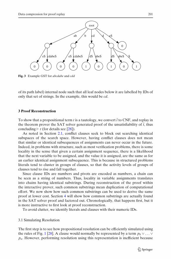
As an example, Fig. 2 gives the GST for the string abcdabe with ID 0, and Fig. 3shows how the GST appears after adding the string cdd with ID 1. The threads arenot shown, and edges are labelled with substrings for readability. It is worth notingthat in Fig. 2, the algorithm has to re-visit branches (the two left-most branches fromthe root node) that were created earlier in the addition of the same string, becausethe substring ab repeats in the string abcdabe. This fact will be of use in Section 4.2.1.

Note that a leaf node is labelled with the IDs of all strings that end at that node.Thus, the longest substring common to a set of strings is the deepest (w.r.t. the length

Fig. 2 Example GSTfor abcdabe root

ab b cd d

0

e$

0

e$

0

cdabe$

0

e$

0

cdabe$

0

abe$

0

abe$


root

ab b cd d

0

e$

0

e$

0

cdabe$

0

e$

0

cdabe$

1

d$

0

abe$

1

d$

0

abe$

1

$

Fig. 3 Example GST for abcdabe and cdd

of its path label) internal node such that all leaf nodes below it are labelled by IDs ofonly that set of strings. In the example, this would be cd.

3 Proof Reconstruction

To show that a propositional term t is a tautology, we convert t to CNF, and replay inthe theorem prover the SAT solver generated proof of the unsatisfiability of t, thusconcluding t (for details see [28]).

As noted in Section 2.1, conflict clauses seek to block out searching identicalsubspaces of the search space. However, having conflict clauses does not meanthat similar or identical subsequences of assignments can never occur in the future.Indeed, in problems with structure, such as most verification problems, there is somelocality in the sense that given a certain assignment sequence, there is a likelihoodthat the next variable to be assigned, and the value it is assigned, are the same as foran earlier identical assignment subsequence. This is because in structured problemsliterals tend to cluster in groups of clauses, so that the activity levels of groups ofclauses tend to rise and fall together.

Since clause IDs are numbers and pivots are encoded as numbers, a chain canbe seen as a string of numbers. Thus, locality in variable assignments translatesinto chains having identical substrings. During reconstruction of the proof withinthe interactive prover, such common substrings mean duplication of computationaleffort. We now show how such common substrings can be used to derive the sameproof at lower cost. Section 4 will show how common substrings are actually foundin the SAT solver proof and factored out. Chronologically, that happens first, but itis more instructive to first look at proof reconstruction.

To avoid clutter, we identify literals and clauses with their numeric IDs.

3.1 Simulating Resolution

The first step is to see how propositional resolution can be efficiently simulated usingthe rules of Fig. 1 [28]. A clause would normally be represented by a term p0 ∨ . . . ∨pn. However, performing resolution using this representation is inefficient because

202 H. Amjad

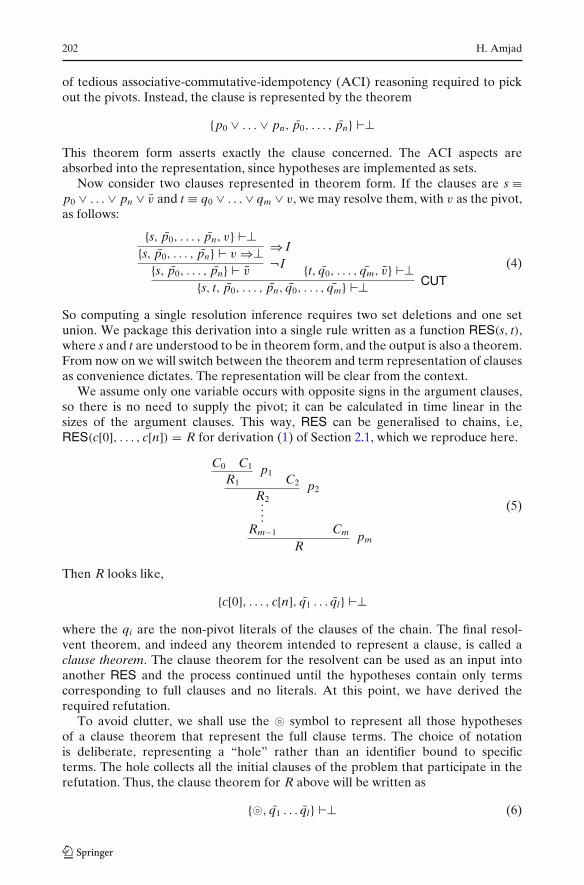
of tedious associative-commutative-idempotency (ACI) reasoning required to pickout the pivots. Instead, the clause is represented by the theorem

{p0 ∨ . . . ∨ pn, p0, . . . , pn} ⊥This theorem form asserts exactly the clause concerned. The ACI aspects areabsorbed into the representation, since hypotheses are implemented as sets.

Now consider two clauses represented in theorem form. If the clauses are s ≡p0 ∨ . . . ∨ pn ∨ v and t ≡ q0 ∨ . . . ∨ qm ∨ v, we may resolve them, with v as the pivot,as follows:

{s, p0, . . . , pn, v} ⊥{s, p0, . . . , pn} v ⇒⊥ ⇒ I

{s, p0, . . . , pn} v¬I {t, q0, . . . , qm, v} ⊥

{s, t, p0, . . . , pn, q0, . . . , qm} ⊥ CUT(4)

So computing a single resolution inference requires two set deletions and one setunion. We package this derivation into a single rule written as a function RES(s, t),where s and t are understood to be in theorem form, and the output is also a theorem.From now on we will switch between the theorem and term representation of clausesas convenience dictates. The representation will be clear from the context.

We assume only one variable occurs with opposite signs in the argument clauses,so there is no need to supply the pivot; it can be calculated in time linear in thesizes of the argument clauses. This way, RES can be generalised to chains, i.e,RES(c[0], . . . , c[n]) = R for derivation (1) of Section 2.1, which we reproduce here.

C0 C1

R1p1

C2

R2p2

....Rm−1 Cm

Rpm

(5)

Then R looks like,

{c[0], . . . , c[n], q1 . . . ql} ⊥where the qi are the non-pivot literals of the clauses of the chain. The final resol-vent theorem, and indeed any theorem intended to represent a clause, is called aclause theorem. The clause theorem for the resolvent can be used as an input intoanother RES and the process continued until the hypotheses contain only termscorresponding to full clauses and no literals. At this point, we have derived therequired refutation.

To avoid clutter, we shall use the � symbol to represent all those hypothesesof a clause theorem that represent the full clause terms. The choice of notationis deliberate, representing a “hole” rather than an identifier bound to specificterms. The hole collects all the initial clauses of the problem that participate in therefutation. Thus, the clause theorem for R above will be written as

{�, q1 . . . ql} ⊥ (6)


3.2 Using Memoised Pieces of Chains

The memoisation algorithm (Section 4) generates a new, memoised proof from theSAT solver proof. It detects shared parts of the proof and writes them out beforetheir first use, and later in the proof at the point of use inserts pointers to the sharedpart. We now show how this sharing is used in the theorem prover.

Let a semi-chain be a strictly alternating sequence of pivots and clauses, startingwith a pivot and ending with a clause. Semi-chains are written using the same linearform as chains. The length or size of a semi-chain is the number of pivots in it. Givena chain c, a semi-chain (ci)c[i] . . . (c j)c[ j ] is denoted by c[i.. j ] for i > 0, analogous tosubstring notation.

We allow semi-chain notation in RES, i.e.,

RES(c[0], c[1], c[2], . . . , c[n])= RES(c[0], c[1..n])= RES(c[0], . . . , c[i − 1], c[i.. j ], c[ j + 1], . . . , c[n])

Further, we use RES(c) for RES(c[0], c[1..n]), and the indexing notation for singlingout chain pivots and clauses is extended to semi-chains.

We plan to use our memoisation algorithm (Section 4) to identify semi-chainscommon to more than one chain in the proof. Suppose the algorithm has found asemi-chain s with m pivots, such that s = c1[i..i + m − 1] and s = c2[i′..i′ + m − 1] forchains c1 and c2.

The aim is compute the resolutions in s only once. The immediate problem is thatthe semi-chain has no first clause with which to begin computing its resolutions. Toget around this, we construct the first clause s for s using the list of pivots of s, asfollows:

{s1 ⇒ . . . ⇒ sm ⇒⊥} s1 ⇒ . . . ⇒ sm ⇒⊥ ASSUME

.... ⇒ E{s1 ⇒ . . . ⇒ sm ⇒⊥, s1, . . . , sm

} ⊥ (7)

By building RES(s, s[1..m]) as shown in Section 3.1, we can confirm that

RES(s, s) = {�, s1 ⇒ . . . ⇒ sm ⇒⊥, q0, . . . , qk

} ⊥where the q literals are the non-pivot literals occurring in the clauses of s.

The only extra term in the hypotheses, which makes it not quite a clause theorem,is s1 ⇒ . . . ⇒ sm ⇒⊥, contributed by the first clause s. Intuitively this term representsthe work done in the computation of the semi-chain, and will be used as a lemmawhen using the semi-chain while computing a chain. This term is then the key to“resolving” away all the pivots ci

1, . . . , ci+m−11 of c1.

Example Let C1 = {0, 1, 2}, C2 = {0, 1, 3} and C3 = {3, 7}, and consider a semi-chain(2)C1(1)C2(3)C3. We have

RES(s, s) = {�, 2 ⇒ 1 ⇒ 3 ⇒⊥, 0, 7} ⊥where � represents the three clauses (and any other clauses that were used in thederivations of those clauses, if those clauses were derived). Note that the non-pivot

204 H. Amjad

literals occur negated, as they should in the theorem version of the clause (e.g., (6) inSection 3.1).

We can now see why semi-chains do not begin with a clause: if they did, the pivotto be removed from that clause would vary from one use of the semi-chain to another,making it impossible to cache RES(s, s). We note the cost of constructing this clause.

Theorem 1 The cost of constructing s is O(|s| log(|s|)).

Proof We need |s| set insertions into a set of size O(|s|) (one for each ⇒ E ofderivation 7). ��

Now, we wish to derive RES(c1[0], c1[1..i + m − 1]) without computingRES(c1[i − 1], c[i..i + m − 1]). The first step is

RES(c1[0], c1[1..i − 1]).... ⇒ I

{�, q0, . . . , qk} s1 ⇒ . . . ⇒ sm ⇒⊥ RES(s, s){�, q0, . . . , qk′ } ⊥ CUT

(8)

where the q literals are again the non-pivot literals of the clauses of c1, up to thatpoint in the derivation. This derivation works because ⇒ I does not require that theantecedent being introduced should occur in the hypotheses of the theorem; if it does,it is deleted from the hypotheses as an additional step.

Example Consider the clause C0 = {2, 8}, and the chain c1 ≡ C0(2)C1(1)C2(3)C3

where C1, C2 and C3 are as in the previous example. Then, using the semi-chainof the previous example, we get

{�, q0, . . . , qk′ } ⊥ ≡ {�, 0, 7, 8} ⊥

We now have a clause theorem at this point, so the derivation can be continued,perhaps using up more non-overlapping semi-chains that matched in c1, until theentire chain has been processed, i.e.,

RES(c1) = RES({�, q0, . . . , qk′ } ⊥, c1[i + m..n])Overlaps will be discussed in Section 3.3. RES(c2) is computed similarly.

In what follows, a match is a pair of chains containing a common semi-chain, whichis then said to have matched in the two chains.

The correctness of our method for using semi-chains is evident in the formalderivations above. However, using semi-chains involves some overhead costs, bothone-off and per-use. The following theorem does not account for overlaps.

Theorem 2 Suppose a semi-chain s of size m is matched M times (for M > 0). LetN be an asymptotic upper bound on the number of literals occurrences in all thechain clauses of all matched chains containing s, up to but not including s[1]. Then thetotal cost of inferences in the natural deduction proof is reduced by MmN − MN −O(m log(m)) − N.


Proof Let c be some chain containing s. First we calculate the one-time net overheadcost for using s. We must construct s, which is O(m log(m)) by Theorem 1, and wemust compute R(s, s) = R(s, c[i..i + m − 1]). Now M > 0 means that s matched in atleast two chains. Consider the very first matched chain, say c, wlog. Then we havesaved in c the computation of R(R(c[0], c[1..i − 1]), c[i..i + m − 1]) (here, we useR(c[0], c[1..i − 1]) to represent an already computed clause theorem). In the worstcase, R(c[0], c[1..i − 1]) still has at least m + 1 elements in the hypotheses (at least mremaining pivots plus at least one more element so that we do not derive the emptyclause in the middle of the chain). But s has exactly m + 1 elements in its hypotheses.Hence the savings cancel out the cost of R(s, s) = R(s, c[i..i + m − 1]. So our net one-time overhead cost so far is O(m log(m)).

To this we must add the cost of using s in c. From derivation 8, this is m setdeletions plus the cost of the set union in R(R(c[0], c[1..i − 1]), R(s, s)) (we ignorethe single set deletion as it will be absorbed by the asymptotic values). We cannotknow a priori the number of elements in the hypotheses of R(c[0], c[1..i − 1]),because we do not know how many non-pivot literals there may be in each chainclause. This number, call it n′, is bound above by the total number of literals inthe chain up to c[i − 1], so n′ = O(�i−1

j |c[ j ]|). Then also, n′ > 2m. Hence the setunion cost is N = O(n′ log(n′)). So the total one-time overhead for the semi-chain isO(m log(m)) + N.

Now we consider the cost per use of the semi-chain. This is just N as calculatedabove. Here, we make the simplifying assumption that n′ is the same for all chainsin which s was matched. This is reasonable approximation since n′ is an asymptoticvalue, and all the matched chains are expected to contain roughly the same clausesdue to locality.

The time savings in each matched chain (other than the first) are mN, sincewithout the semi-chain there would have been m resolution steps to compute, eachresolution’s set union costing N in the limit.

Thus, the total time saved over M matches is MmN − MN − O(m log(m)) − N.��

Since the cost reduction could be negative due to the overhead, we must balancethe overhead against the time savings from using the semi-chain. This is discussedfurther in the next section.

3.3 Merging Overlapping Semi-chains

When a semi-chain s matches in at least two chains, it is written out to the proofbefore the chains which will use it. The chains that use s have the s part of themselvesreplaced by a semi-chain of size one, consisting of the first pivot of s and a clause IDthat points to RES(s, s) in the clause database.

This becomes problematic when semi-chains overlap. Although it is fine to useover-lapping semi-chains using the method of the previous section, it is unsatisfactorybecause the ⇒ I inferences of derivation 8 will waste time attempting to remove non-existent pivots.

We show how to merge two overlapping semi-chains to avoid this wasted com-putation; it is easy to extend the method to more than two. We assume that the

206 H. Amjad

semi-chains do overlap and that neither is contained entirely within the other. Thememoisation algorithm will guarantee this.

Suppose in a chain c we have we have two overlapping semi-chains s1 = c[i1.. j1]and s2 = c[i2.. j2], where i1 < i2. The merged semi-chain, s3, is then c[i1.. j2]. We firstcompute the list of pivots of s3, [ci1 , . . . , c j2 ]. The next step is to construct the clauses3. This is done exactly as in derivation 7 of Section 3.2, except that we now use thelist we just computed. Once that is done, RES(s3, s3) is derived by

s3.... ⇒ I

{�, q0, . . . , qk} ci1 ⇒ . . . ⇒ c j1 ⇒⊥ RES(s1, s1)

{�, q0, . . . , qk′ , ci1 ⇒ . . . ⇒ c j2 ⇒⊥} ⊥ CUT.... ⇒ I

{�, q0, . . . , ¯qk′′ } ci2 ⇒ . . . ⇒ c j2 ⇒⊥ RES(s2, s2)

{�, q0, . . . , ¯qk′′′ , ci1 ⇒ . . . ⇒ c j2 ⇒⊥} ⊥ CUT

(9)

where the q literals are again the non-pivot literals, and RES(s1, s1) and RES(s2, s2)

have already been computed using derivation 8 of Section 3.2. It is tedious but nothard to show that this clause theorem is precisely the clause theorem that would begenerated from scratch (i.e., by performing all the resolutions) for the semi-chain s3.RES(c) can now be computed as in derivation 8 of Section 3.2, using RES(s3, s3).

While the time savings for using a semi-chain were calculated over the entireproof, each merge is specific to a single chain. To determine our profit from themerge, we can restrict our attention to a single chain. We consider only a mergeof two semi-chains, extensions to more than two being straightforward.

Theorem 3 With the merged semi-chain s3, the decrease in the number of inferences isN0 − N1 − N2, where N0, N1 and N2 are asymptotic upper bounds on all literals in thechain clauses of c, up to but not including s1[1], from s1[1] to s1[|s1|], and from s2[1] tos2[|s2|] respectively.

Proof We cannot offset merge overheads against the savings from using RES(s1, s1)

and RES(s2, s2) since these have already been used up in analysing the cost of usingsemi-chains, and here we wish to see what additional effect merging has. Thereforewe can only consider constructions involving the merged semi-chain, and offsetagainst uses of s1 and s2 in c, which the merge replaces.

Let m = |s3| log(|s3|). The time saved by not performing the vacuous ⇒ I infer-ences is cancelled out by the extra time taken to construct s3: both are O(m). Thetwo uses of s1 and s2 in constructing s3 (see derivation 9) cost O(m) + N1 andO(m) + N1 + N2 respectively. The use of s3 in c costs N0 + N1 + N2. On the otherhand, without merging, the uses of s1 and s2 in c cost (N0 + O(m) + N1) + (N0 +N1 + O(m) + N2). Subtracting the total cost O(m) + N1 + O(m) + N1 + N2 + N0 +N1 + N2 from this, we have the result. ��

This result can be easily generalised to multiple overlapping chains, specially sincethe memoisation algorithm drops semi-chains that are completely covered by otherchains. The savings in time occur because the number of all the literals of clauses


encountered up to but not including s1, tends to be higher than the number of literalsin all the clauses of s1 and s2, specially as these semi-chains overlap.

Sadly, our problems with overlaps do not end here: the computation ofRES(s1, s1)

and RES(s2, s2) computes the overlapping resolutions twice. This is a difficultproblem because redundant computations of this type are not necessarily local to asingle chain. Currently we add some trade-off analysis to the memoisation algorithmto ameliorate the situation (see Section 4.2) but the general problem has not beensolved. We cannot, of course, discard s1 and s2 in favour of s3, since they areseparately used elsewhere.

4 Proof Memoisation

We now turn to the generation of the memoised proof itself. The input is the SATsolver generated proof (from which unused chains have already been filtered out).The output is a memoised proof that factors out shared semi-chains and additionallyindicates when merging is required.

Since SAT solver proofs can have millions of inferences, we need an efficientway of detecting shared semi-chains. The algorithm proceeds in three stages. In thenormalisation stage, we preprocess the chains to increase the likelihood of findingidentical semi-chains. In the match stage, we make a pass though the proof, addingchains to a GST and collecting information about matches. In the write stage, wewrite out the memoised proof, ensuring that all semi-chains are written out beforetheir point of first use.

4.1 Normalisation

As noted in Section 3, locality in structured problems causes identical subsequencesof variable assignments to take place in different parts of the SAT solvers searchtree. Sometimes however, the subsequences are almost but not quite the same.Specifically, two subsequences may have the same set of assignments but in adifferent order. The reason for this is that a unit propagation step can cause morethan one clause to become unit, in which case the next variable to propagate ischosen heuristically based on various metrics, such as clause activity levels. Theselevels change during search, and so it is possible that the order in which variables arepicked for the next propagation step changes slightly. The aim of the normalisationstage is to re-order assignment sequences so that, whenever possible, subsequencesof assignments that differ only in order of assignment become identical.

Re-ordering of assignment sequences is the same as re-ordering the (pivot,clause)pairs in a chain. Re-ordering cannot be done across multiple chains because thatwould mean conflating different branches of the SAT solver search tree: each chaincorresponds to a conflict clause derivation and the solver will not descend further ona branch which contains a conflict.

The idea behind re-ordering is to choose an arbitrary global ordering < on pivots(hence “normalisation”), and then sorting each chain’s (pivot,clause) pairs by pivot.This is easily done since pivots are literals and so are represented by unique numbers.

The problem is harder than a simple sort however, because pivots once removedfrom a chain must not be re-introduced. To do so would defeat the aim of resolving

208 H. Amjad

them out in the first place. Thus, the sort cannot move a pivot to a position earlierthan its last complementary occurrence in a chain clause. It is not possible to modifythe global pivot ordering < to get around this problem. For instance, consider thesemi-chains s1 ≡ (p0)C0(p1)C1 and s2 ≡ (p1)C2(p0)C3, where p1 ∈ C0 and p0 ∈ C2.Then in the modified global ordering <′, s1 will require that p0 <′ p1, whereas s2

will require that p1 <′ p0. Of course, it defeats the purpose of normalisation to usedifferent sort orderings for each chain.

The answer is to track dependencies between the clauses of a chain, and thenperform a topological sort. Unlike the rest of the proof memoisation algorithm, thisis the only point at which we need to examine the actual literals of the clauses.

Let G be the dependency graph of a chain c. The nodes GV of G are the pivots ofthe chain (no pivot occurs twice in the same chain; see restriction (1) at the end ofSection 2.1). The arcs GA of G are defined as follows: for every (pivot,clause) pair(ci, c[i]), if ci ∈ c[ j ] for some j, then there is an arc (c j, ci) ∈ GA. Since ci is never re-introduced after its removal via resolution with c[i] (see restriction (2) at the end ofSection 2.1), we have that j < i and so G is acyclic. Since for each ci there is at leastone clause c[ j ] such that ci ∈ c[ j ], G is connected.

G is easily constructed in time O(�i|c[i]|) simply by scanning all the clauses. Letmin(S) return the minimum (with respect to the global total ordering on pivots) of aset S of numbers, and let the in-degree of a graph node be the number of incomingarcs [7]. Once we have G, the re-ordered chain c′ is constructed as follows:

1. c′ ← c[0]2. ci ← min{ci|ci ∈ GV ∧ in-degree(ci) = 0}3. GV ← GV − ci

4. foreach (ci, p) ∈ GA

GA ← GA − (ci, p)

5. c′ ← c′(ci)c[i]6. if GV = ∅ then return c′ else goto 2

Note that we are implicitly tracking dependencies between clauses as claimed, aseach chain clause (except the first) is uniquely associated with a pivot. The verticesare maintained in an ordered set, sorted on in-degree. Whenever a vertex p isremoved, all vertices to which it had arcs are removed from the set, their in-degreesdecremented, and re-inserted into the set.

Example Consider the chain {1, 2, 3}(3){1, 3}(2){1, 2}(1){1} which derives the emptyclause. Let the global ordering on literals (and hence on pivots) be 1 < 1 < 2 < 2 <

3 < 3. Then G is

2

1

3


and the re-ordered chain is {1, 2, 3}(2){1, 2}(3){1, 3}(1){1} where the pivot 2 has beenmoved before the pivot 3 to respect the ordering, but pivot 1 cannot be movedwithout changing the clause derived by the chain.

We now consider correctness.

Theorem 4

RES(c) = RES(c′)

Proof The construction of c′ proceeds by removing vertices, or pivots, from thegraph and appending the corresponding (pivot,clause) pair to the end of c′. Step 2 ofthe construction of c′ ensures only source vertices are removed. Since G is a DAG,there is always at least one source vertex after each removal. By the definition ofGA, the pivot corresponding to the vertex being removed, say p, does not have anycomplementary occurrences left among the clauses corresponding to the remainingvertices. So all c[ j ] such that p ∈ c[ j ] have already been added to c′. Hence ateach step in the computation of RES(c′), once a pivot p is removed it is never re-introduced. So when the computation completes, the only literals left are the non-pivot literals of the clauses of c′, and these are precisely the non-pivot literals of theclauses of c. ��

Normalisation achieves the best possible result at relatively low cost. We provethe complexity result for normalisation, assuming set insertion and deletion islogarithmic.

Theorem 5 Normalisation of a chain c takes time O(|c|2 log(|c|) + �i|c[i]|).

Proof The cost of constructing G is O(�i|c[i]|), a linear scan of all literals of allclauses of c. In the worst case, G will always contain exactly one source, before andafter each vertex removal from V (except the last removal). This corresponds to thesituation where each clause contains all the remaining unremoved pivots. In this case,for each removal, O(|c|) vertices must be updated. Each update requires a constanttime in-degree decrement, a set deletion and an insertion, giving O(log(|c|)) updatecost. There are |c| pivots to remove giving O(|c|2 log(|c|)). ��

In practice the worst case rarely ever occurs. Typically, the in-degree of a vertexis 1, and the time taken by normalisation is a negligible component of overall time.

4.2 Matching: Detecting Shared Semi-Chains

Let V be the set of literals (hence potential pivots) and C be the set of clause IDs.Then our alphabet A is V + C, the + here indicating disjoint union. Every semi-chainis a string, but not all strings are semi-chains. A sub-semi-chain of a semi-chain is anysubstring of the semi-chain that begins at an even numbered index (string indexesbegin at zero) and is of even length.

In the match stage, our strategy will be to drop the first clause from each chainwe encounter, and add the resulting semi-chain to our GST, as a string. Then, whenreading in later chains, we shall match in the GST the longest sub-semi-chain(s) of

210 H. Amjad

the chain being read. Since not all strings (and hence not all substrings) are semi-chains, we will need to modify the GST matching algorithm to return only valid semi-chains. We could let (literal,clause ID) pairs be the alphabet, but then A = V × Cand the constant factors in the complexity results would go from log2(|V| + |C|) tolog2(|V||C|) (see Section 2.3).

The modification is easily done by filtering matching substrings. When the GSTreturns a match, it is possible to check in constant time that the starting index of thematch is even numbered in both matching chains, and that the length of the match iseven. If so, it is a valid semi-chain.

4.2.1 Detecting a Match

In Section 2.3 we noted the longest common substring is the path label of thedeepest node below which all leaves are marked only with the IDs of the stringswe are interested in. This requires the use of sophisticated lowest common ancestoralgorithms [13]. Fortunately, we are interested in finding a match with any string, toonly the string currently being added. So we can limit ourselves to leaves markedwith the ID of the current string. But we can do better.

We know that a pivot never occurs twice in a (semi-)chain (see restriction (1)at the end of Section 2.1). This means that the GST algorithm, when adding thecurrent string, will never revisit a node that was created earlier during the additionof the same string [27]. Nodes (or leaf edges from the root) are created whenever weare unable to find a way to extend a suffix of a prefix of the current string withoutexplicitly adding the next character in that suffix to the current path in the treethat we have followed from the root node. This means that the suffix up to but notincluding the next character is a substring of an earlier chain, as well as a substring ofthe chain being added.

So, thanks to our knowledge of the structure of the strings, we can detect matcheson the fly as we add the current string. The parent edge of any node just created waslabelled with the ID of the string (or equivalently, the clause ID of the chain) duringthe addition of which that edge was created. This string/chain is called the owner ofthe match, and we are guaranteed not only that it contains the matched semi-chain,but also that it is the very first string that contains the matched semi-chain, sinceedges’ string ID labels are assigned only when the edge is created.

4.2.2 Choosing the Best Match

Adding a string can return multiple overlapping matches. We have considered threedifferent schemes for retaining these matches:

1. Retain only the longest size match.2. Retain all matches.3. Greedily retain maximal non-overlapping matches.

Since each retained match is converted into a memoised semi-chain in the outputproof, the retention scheme affects how much merging will be required. Scheme 1minimises merging (merging can still occur, in the owning chain), but may miss manyopportunities for sharing work. Scheme 2 does not miss anything, but maximisesmerging. Scheme 3 attempts to find a middle of the road solution, and in experimentsso far it appears to be superior.


It is too expensive to find the optimal maximal non-overlapping matches. Matchesare always reported in increasing order of starting index (recall the GST algorithmconsiders prefixes of increasing size), so Scheme 3 adopts a greedy approach asfollows, where set R is the set of reported matches that will be returned by the GST,and s is the string being added:

1. R ← ∅, M ← ∅, max j ← −1

2. s[i.. j ] ← next_match

3. if i > max j then R ← R ∪ {max_substring(M)}, M ← {s[i.. j ]}else M ← M ∪ {s[i.. j ]}, max j ← max( j, max j)

4. if last_match then R ← R ∪ {max_substring(M)}else goto 2

For each match that is reported, pointers to information about the match arerecorded keyed on both the current and the owning string, for use during the writestage. These are literally pointers, so there is no wasted memory.

4.2.3 Trade-Off Analysis

Using the results of Theorem 2 and Theorem 3, we can determine to some degree theminimal bounds on semi-chain sizes, number of matches and sizes of overlaps, thatguarantee a profitable result.

We do not report matches of length two, since these correspond to semi-chains oflength one. In that case, the overhead for using the semi-chain outweighs the savings.The situation is slightly more complicated for semi-chains of length two. Here, if wehave only a single match, the overhead cost is greater than the savings. However, if asemi-chain of length two matches in more than two chains, then we make a net profitin terms of set unions saved. For semi-chains of length three or more, we alwaysprofit (ignoring merges for the moment).

It is worth noting how we keep a count of how many times a semi-chain hasmatched. This information is used in the write stage to decide which matches toretain, because by then we know how many times every semi-chain matched. Thesemi-chain match count information is recorded in a map whose key is a 64 bitunsigned integer constructed as follows:

1. The first 32 bits give the owner string’s ID2. The next 16 bits give the starting index in the owner3. The next 16 bits give the ending index in the owner

This hash is perfect because a distinct matched semi-chain will always be owned bythe string of the very first chain to contain that semi-chain. 32 bits for the clause IDis sufficient. 16 bits for the indices is not as safe, though we have yet to come acrossany proofs where a conflict clause derivation contained more than 216 pivots.

4.3 Writing: Merging and Splitting

Once the match stage is over, we have for each chain information on all its matches,including those for which it is the owner. We now make another pass through the

212 H. Amjad

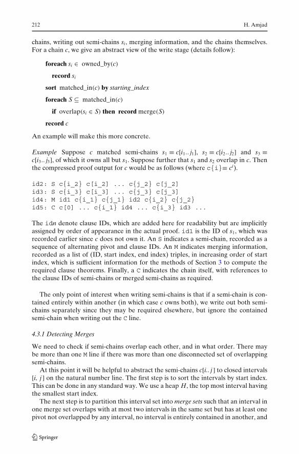
chains, writing out semi-chains si, merging information, and the chains themselves.For a chain c, we give an abstract view of the write stage (details follow):

foreach si ∈ owned_by(c)

record si

sort matched_in(c) by starting_index

foreach S ⊆ matched_in(c)

if overlap(si ∈ S) then record merge(S)

record c

An example will make this more concrete.

Example Suppose c matched semi-chains s1 ≡ c[i1.. j1], s2 ≡ c[i2.. j2] and s3 ≡c[i3.. j3], of which it owns all but s1. Suppose further that s1 and s2 overlap in c. Thenthe compressed proof output for c would be as follows (where c{i}≡ ci).

id2: S c{i_2} c[i_2] ... c{j_2} c[j_2]id3: S c{i_3} c[i_3] ... c{j_3} c[j_3]id4: M id1 c{i_1} c{j_1} id2 c{i_2} c{j_2}id5: C c[0] ... c{i_1} id4 ... c{i_3} id3 ...

The idn denote clause IDs, which are added here for readability but are implicitlyassigned by order of appearance in the actual proof. id1 is the ID of s1, which wasrecorded earlier since c does not own it. An S indicates a semi-chain, recorded as asequence of alternating pivot and clause IDs. An M indicates merging information,recorded as a list of (ID, start index, end index) triples, in increasing order of startindex, which is sufficient information for the methods of Section 3 to compute therequired clause theorems. Finally, a C indicates the chain itself, with references tothe clause IDs of semi-chains or merged semi-chains as required.

The only point of interest when writing semi-chains is that if a semi-chain is con-tained entirely within another (in which case c owns both), we write out both semi-chains separately since they may be required elsewhere, but ignore the containedsemi-chain when writing out the C line.

4.3.1 Detecting Merges

We need to check if semi-chains overlap each other, and in what order. There maybe more than one M line if there was more than one disconnected set of overlappingsemi-chains.

At this point it will be helpful to abstract the semi-chains c[i.. j ] to closed intervals[i, j ] on the natural number line. The first step is to sort the intervals by start index.This can be done in any standard way. We use a heap H, the top most interval havingthe smallest start index.

The next step is to partition this interval set into merge sets such that an interval inone merge set overlaps with at most two intervals in the same set but has at least onepivot not overlapped by any interval, no interval is entirely contained in another, and


no interval overlaps with an interval in another merge set. The intuition is that eachmerge set corresponds to a single M line. Merge sets keep their intervals sorted bystart index. The merge sets are created as follows, where L is the final list of mergesets (@ is list append):

1. L ← [∅]2. if empty(H) then return L else [i, j] ← pop(H)

3. if j − i = 1 ∧ times_matched(c[i.. j ]) = 1 then goto 2

4. [i′, j ′] ← last(last(L))

5. if j ′ ≥ i

if j ≤ j ′ ∨ i′ ≥ i then last(L) ← last(L) ∪ {[min(i, i′), max( j, j ′)]}else last(L) ← last(L) ∪ {[i, j ]}

else L ← L@{[i, j ]}6. goto 2

Note we take care to filter out intervals contained entirely within others. Thisprocedure is linearithmic in the number of intervals. It is inspired by a computationalgeometry data structure called an interval tree [5]. Since we only have to make onepass through the intervals, we do not need to construct the tree explicitly.

4.3.2 Splitting Merged Semi-Chains

At this point we are ready to write out the merge information, each merge setin L contributing one M line. However, recall that we wish to avoid overlapsaltogether if possible, because then the resolutions in the overlapping part arecomputed twice, once for each semi-chain. We can sometimes avoid this situationby splitting two overlapping semi-chains into three semi-chains, corresponding tothe non-overlapping part of the first semi-chain, the overlapping part, and the non-overlapping part of the second semi-chain. The three new semi-chains do not requiremerging, since they do not overlap, and the overlapped part is now computed onlyonce.

Since semi-chains matched in c but not owned by c, have already been writtenout, a split can only happen if both the involved semi-chains are owned by c.This considerably limits our trade-off analysis, because in general we have no ideawhether a given semi-chain overlaps another that is owned by some other chainthat the write stage has yet to encounter. Part of the problem is that GSTs do noteliminate suffix redundancy, so there may be more than one owner of some suffixstring of a semi-chain. We are in the process of fixing this deficiency using wordgraphs [19].

Even when we can split an overlap, it does not always pay to do so. The resultingsemi-chains could be of length two, so that using them may result in a net increase incomputational effort. Further, if there is a choice between which overlap to split, weneed to be careful since that split could affect whether or not we split any remainingoverlaps.

214 H. Amjad

Therefore, for each merge set, we adopt a greedy approach: we sort overlaps bysize, and begin by splitting the biggest one, for maximum savings. We avoid splittingoverlaps where the resulting middle semi-chain would be of size two or less. Thesplitting information does not have to be recorded in the proof: all we get is a fewmore S lines and few less M lines. This optimisation made a marked difference inpractice.

5 Experimental Results

Since the shortening of resolution proofs is believed to be an intractable problem [1],the algorithm is of heuristic value only, and requires benchmarking for evaluatingoverall time savings. The best we could do, and have done, is provide analyticalcomplexity analysis at the chain level.

In practice, the match and write stages are almost linear in the length of theproof: the match stage adds chains and detects matches in time linear in the lengthof the chain, and analysis of merging information in the write stage for each chaintakes worst case linearithmic time in the number of semi-chains matched in thatchain. Though we cannot give an analytical account, the latter number is typicallydominated by the size of the chain itself.

The preprocessing normalisation stage has different behaviour because it inspectsthe literals of the clauses. Thus in problems with large clauses, preprocessing can besignificantly more expensive than in problems with small clauses.

We tried out our algorithm on a few problems from the SATLIB benchmarkslibrary for SAT solvers. We used the ZChaff SAT solver [22] to generate the proofs,which were then memoised using a C++ implementation, and then reconstructedin HOL4. The results are summarised in Table 1. The columns are, respectively:problem name, number of variables, number of clauses, SAT solver time, proofreplay time, compression time, compressed proof replay time, number of resolutions,number of resolutions in compressed proof, net speed up. The benchmark machinewas an Intel P4 3GHz CPU with 4GB of RAM. Times are in seconds.

The missing HOL4+M time for ip50 is due to an internal runtime error in theruntime engine of Moscow ML, on top of which HOL4 executes. Developers havebeen notified.

As hoped, the proof replay times in the theorem prover do improve when using thememoising algorithm. The payoff column measures the reduction in total time andis always positive. Of course, were we to verify the proofs in, say, C++, the payoffwould almost certainly be less, because compression time would then be a greaterportion of verification time. However our aim here is not to debug SAT solvers, butto use them as untrusted oracles for fully expansive theorem provers. The latter arenot engineered for large resolution proofs, so we expect the payoff to be positiveregardless of the implementation language.

It would be uninformative to compare a C++ verifier for our compressed proofsagainst a C++ verifier that directly verifies the original SAT solver proof. This isbecause the direct verifier can quickly verify the proof using a single linear timehyperresolution step per chain [29]. System N cannot efficiently simulate hyper-resolution (this is easily seen since N cannot eliminate more than one connectiveper inference; see Section 2.2). Since our entire motivation is to use SAT solvers


Tab

le1

Tim

esin

seco

nds

Pro

blem

Var

sC

laus

esZ

Cha

ffH

OL

4M

emo

HO

L4+

MR

esR

es+

MP

ayof

f

am_5

_510

7636

7744

384

2330

321

0989

618

5071

215

%c7

552.

mit

er11

282

6952

978

104

376

2425

0922

5439

24%

desm

ul.m

iter

2890

217

9895

364

6515

6930

0013

1256

011

1868

852

%ip

3647

273

1533

6821

817

0622

1219

1141

756

1022

449

27%

ip38

4996

716

2142

237

1831

2312

2211

0993

299

6248

32%

ip50

6613

121

4786

1077

9034

118

–39

5797

335

6836

2–

6pip

e15

800

3947

3920

039

67

286

3108

1326

7972

26%

6pip

e.oo

o17

064

5456

1238

410

9315

735

7829

0369

4019

31%

7pip

e23

910

7511

1858

410

1019

793

4970

1943

7060

20%

term

1mul

3504

2222

940

534

927

279

1546

075

1424

546

12%

vdam

ul54

4434

509

1641

5841

290

3400

3846

386

3451

297

37%

Res

olut

ions

inin

fere

nce

step

s.P

ayof

fin

%ti

me

216 H. Amjad

with theorem provers for N, the output of our compression algorithm must avoidusing hyperresolution. It is unclear what a semi-chain means in the context ofhyperresolution, so writing a hyperresolution based verifier for compressed proofsmay be non-trivial. Even if we could, the compression algorithm breaks up chains sothat verifiers for compressed proofs would only be able to use a mix of resolution andhyperresolution, slowing them down. Thus the comparison would be uninformative.

We have not yet compared our method against other SAT solver proof compres-sion methods we are aware of [10, 26]. One reason is that both of them performsemantic analysis, which is considerably harder than our syntactic analysis. Thus thespeed comparison would be strongly skewed in our favour (we have verified thisobservation on a few test cases). This would be unfair, since their aims are differentfrom ours. Indeed, [10] does not even output the compressed proof (they areinterested only in removing redundant problem clauses), whereas [26] changes thetarget proof system to extended resolution. So simply figuring out how to verify theiroutput using system N may require considerable further research and engineering.

As expected, the number of resolution steps is also lower in the memoised proof.This does not tell the full story for two reasons:

1. The number of resolutions will not necessarily correlate with proof replay timebecause the time taken by each resolution depends on the sizes of the argumentclauses.

2. The memoised proof contains inferences other thanRES inferences. Rather thancounting all the different kinds of inferences, we normalised the computationalcost in terms of set unions, deletions and insertions. The memoised proofshave more primitive inferences, but after factoring out the inferences due tosimulating RES, we observed that the remaining inferences are mostly setdeletions/insertions due to first clause construction and merging for semi-chains.These operations are cheaper than set unions, so we conclude that the timesavings come from the reduction in the number of costly set unions that occurin applications of the RES rule.

SAT solvers are a mature and successful technology. The levels of redundancy wehave found in the proofs (and that too after retaining only that part of the solver’ssearch that actually participates in the final proof) give us hope that more can beachieved as our algorithm matures.

6 Conclusion

Other than the already cited work [9, 28] we are not aware of any work on integrationof DPLL based SAT solvers with interactive theorem provers. Harrison integrateda SAT solver based on Stålmarck’s method into HOL90 [16], and the theoremprovers PVS, Coq and HOL Light have been integrated with SMT solvers at varioustimes. Certainly, we are not aware of any work on memoisation of SAT solvergenerated proofs. The closest work we could find is on merging chains using extendedresolution, but both the method and the aim of that work are completely differentfrom our own [26].


Our first next will be to address the issue of overlapping semi-chains with differentowners, by analysing the structure of the proof, implementing a single owner policy,and using word graphs to eliminate suffix redundancy.

In the longer term, we hope to use this method as one of many in a pipeline ofproof compressors (e.g., [10, 26]) to compress the proof even further. The advantageof our method compared to those cited, is that it is very fast. The disadvantageis that it does not look at the semantic structure of the proof, i.e., implicationsamong clauses, and so possibly misses opportunities for simplification. We expectthe pipeline will address this deficiency.

References

1. Alekhnovich, M., Razborov, A.A.: Resolution is not automatizable unless W[P] is tractable. In:FOCS, pp. 210–219. IEEE, Piscataway (2001)

2. Biere, A., Cimatti, A., Clarke, E.M., Zhu, Y.: Symbolic model checking without BDDs. In:Cleaveland, R. (ed.) Tools and Algorithms for Construction and Analysis of Systems. LNCS,vol. 1579. Springer, New York(1999)

3. Bryant, R.E., Lahiri, S., Seshia, S.: Modeling and verifying systems using a logic of counterarithmetic with lambda expressions and uninterpreted functions. In: Brinksma, E., Larsen, K.G.(eds.) Proc. 14th Intl. Conference on Computer Aided Verification. LNCS, vol. 2404, pp. 78–92.Springer, New York (2002)

4. Clarke, E., Kroening, D., Lerda, F.: A tool for checking ANSI-C programs. In: Jensen, K.,Podelski, A. (eds.) Tools and Algorithms for the Construction and Analysis of Systems (TACAS2004). LNCS, vol. 2988, pp. 168–176. Springer, New York (2004)

5. Cormen, T.H., Leiserson, C.E., Rivest, R.L., Stein, C.: Introduction to Algorithms. MIT,Cambridge (2001)

6. Davis, M., Logemann, G., Loveland, D.: A machine program for theorem proving. J. Assoc.Comput. Mach. 5(7), 394–397 (1962)

7. Diestel, R.: Graph Theory. Springer, New York (2005)8. Eén, N., Sörensson, N.: An extensible SAT-solver. In: Giunchiglia, E., Tacchella, A. (eds.)

Theory and Applications of Satisfiability Testing, 6th International Conference. LNCS, vol. 2919,pp. 502–518. Springer, New York (2003)

9. Fontaine, P., Marion, J.-Y., Merz, S., Nieto, L.P., Tiu, A.F.: Expressiveness + automation +soundness: towards combining SMT solvers and interactive proof assistants. In: Hermanns, H.,Palsberg, J. (eds.) TACAS. LNCS, vol. 3920, pp. 167–181. Springer, New York (2006)

10. Gershman, R., Koifman, M., Strichman, O.: Deriving small unsatisfiable cores with dominators.In: Ball, T., Jones, R.B. (eds.) Computer Aided Verification. LNCS, vol. 4144, pp. 109–122.Springer, New York (2006)

11. Gordon, M.J.C., Melham, T.F. (eds.) Introduction to HOL: a Theorem-Proving Environment forHigher Order Logic. Cambridge University Press, Cambridge (1993)

12. Gusfield, D.: Algorithmson String, Trees, and Sequences. Cambridge University Press,Cambridge (1997)

13. Harel, D., Tarjan, R.E.: Fast algorithms for finding nearest common ancestors. SIAM J. Comput.13(2), 338–355 (1984)

14. Harrison, J.: Metatheory and Reflection in Theorem Proving: a Survey and Critique. TechnicalReport CRC-053, SRI International (1995)

15. Harrison, J.: HOL light: a tutorial introduction. In: Srivas, M.K., Camilleri, A.J. (eds.) FMCAD.LNCS, vol. 1166, pp. 265–269. Springer, New York (1996)

16. Harrison, J.: Stålmarck’s algorithm as a HOL derived rule. In: von Wright, J., Grundy, J.,Harrison, J. (eds.) Theorem Proving in Higher Order Logics. LNCS, vol. 1125, pp. 221–234.Springer, New York (1996)

17. Hickey, J., Nogin, A., Constable, R.L., Aydemir, B.E., Barzilay, E., Bryukhov, Y., Eaton, R.,Granicz, A., Kopylov, A., Kreitz, C., Krupski, V., Lorigo, L., Schmitt, S., Witty, C., Yu, X.:Metaprl—a modular logical environment. In: Basin, D.A., Wolff, B. (eds.) TPHOLs. LNCS,vol. 2758, pp. 287–303. Springer, New York (2003)

218 H. Amjad

18. Huet, G., Kahn, G., Paulin-Mohring, C.: The Coq Proof Assistant: a Tutorial: Version 7.2.Technical Report RT-0256, INRIA (2002)

19. Inenaga, S., Hoshino, H., Shinohara, A., Takeda, M., Arikawa, S., Mauri, G., Pavesi, G.: On-line construction of compact directed acyclic word graphs. Discrete Appl. Math. 146(2), 156–179(2005)

20. Mitchell, D.G.: A SAT solver primer. In: EATCS Bulletin. The Logic in Computer ScienceColumn, vol. 85, pp. 112–133. Springer, New York (2005)

21. Morrison, D.R.: PATRICIA-practical algorithm to retrieve information coded in alphanumeric.J. Assoc. Comput. Mach. 15(4), 514–534 (1968)

22. Moskewicz, M.W., Madigan, C.F., Zhao, Y., Zhang, L., Malik, S.: Chaff: engineering an efficientSAT solver. In: Proceedings of the 38th Design Automation Conference, pp. 530–535. ACM,New York (2001)

23. Owre, S., Rushby, J.M., Shankar, N.: PVS: a prototype verification system. In: Kapur, D. (ed.)11th International Conference on Automated Deduction (CADE). LNAI, vol. 607, pp. 748–752.Springer, New York (1992). http://pvs.csl.sri.com

24. Paulson, L.C.: Isabelle: a Generic Theorem Prover. LNCS, vol. 828. Springer, New York (1994)25. Shankar, N.: Using decision procedures with a higher-order logic. In: Boulton, R.J., Jackson, P.B.

(eds.) Theorem Proving in Higher Order Logics, LNCS, vol. 2152, pp. 5–26. Springer, New York(2001)

26. Sinz, C.: Compressing propositional proofs by common subproof extraction. In: Pichler, F. (ed.)Euro Conference on Computer Aided Systems Theory, Las Palmas de Gran Canaria, 12–16February 2007

27. Ukkonen, E.: Online construction of suffix trees. Algorithmica 14(3), 249–260 (1995)28. Weber, T., Amjad, H.: Efficiently checking propositional refutations in HOL theorem provers.

JAL (2008). doi:10.1016/j.jal.2007.07.00329. Zhang, L., Malik, S.: Validating SAT solvers using an independent resolution-based checker:

practical implementations and other applications. In: DATE, pp. 10880–10885. IEEE ComputerSociety, Los Alamitos (2003)

http://pvs.csl.sri.com

http://dx.doi.org/10.1016/j.jal.2007.07.003

Documents

Data Compression for Proof Replay