DAAAM INTERNATIONAL SCIENTIFIC BOOK 2010 pp. · PDF fileApplication of Genetic Algorithms in Inventory Management, ... establish the basic EOQ model using Genetic Algorithms ... GAs

DAAAM INTERNATIONAL SCIENTIFIC BOOK 2010 pp. 245-258 CHAPTER 25

APPLICATION OF GENETIC ALGORITHMS IN

INVENTORY MANAGEMENT

DANIA, W.A.P.

Abstract: Inventory cost is a main component of total logistic costs. To achieve the

minimum logistic costs, company needs to manage the amount of carrying inventory

accurately to minimize the impact of the fluctation of demand. In order to deal with

the fluctuation of the demand that creates a mismatch between supply and demand,

Genetic Algorithms are applied to define the optimal solution based on periodic

review system. Genetic Algorithms as one of the optimization method are chosen

because it can handle the problem with highly constrained, multi criteria, multi

combinatorial problem and has large solution. There are several steps that need to

be accomplished to achieve the objective. First, mathematic model of inventory

management which contain of all cost component need to be determined. Second,

based on the proposed mathematic model, Genetic Algorithms as the optimization

method is developed. Finally, the result of Genetic Algorithms is applied in real case

study which is case inone of biscuits companies in Indonesia.

Key words: inventory management, periodic review system, genetic algorithms

Authors´ data: STP, MEng. Dania, W[ike] A[gustin] P[rima], Brawijaya University,

Jalan Veteran Malang 65145, Indonesia, [email protected]

This Publication has to be referred as: Dania, W[ike] A[gustin] P[rima] (2010).

Application of Genetic Algorithms in Inventory Management, Chapter 25 in

DAAAM International Scientific Book 2010, pp. 245-258, B. Katalinic (Ed.),

Published by DAAAM International, ISBN 978-3-901509-74-2, ISSN 1726-9687,

Vienna, Austria

DOI: 10.2507/daaam.scibook.2010.25

245

Dania, W. A. P.: Application of Genetic Algorithms in Inventory Management

1. Introduction

High competition that happens at industry level forces the company to have high

responsiveness to the customer demand and to have high service level. Moreover,

they can also meet the short lead time. One of the factors that have high impact to the

responsiveness of the customer demand is the availability of raw material. Company

needs to maintain a proper inventory level so it can fulfill customer demand and

avoid the delay in production process. Because lead time depends on the effort of the

suppliers, therefore good inventory management in company stage must be managed

effectively.

Inventory is accumulated materials for supporting manufacturing system that includes

production, distribution, and operating support (Starr 2007). Hill (2005) states that

the general role of the inventory is to separate various stages in manufacturing

systems that are not synchronized, allowing them to work in their own space.

Therefore, company carries the appropriate inventory to meet the customers demand

and to avoid material shortages. Stock and Lambert (2001) point out that the purpose

of holding inventory is to accomplish the ‘economy of scale’ in all stages of

manufacturing. They also mention that inventory can solve the mismatch between

supply and demand, handle the demand uncertainty, and as a buffer when there is

order beyond the forecasted demand.

Inventory cost is one of the main components of a manufacturing company’s total

cost. Heizer and Render (1993) mention that inventory comprises 40% of total

manufacturing cost. Therefore, to reduce the total cost significantly, one of the

solutions is minimizing the inventory cost without reducing the quality of its output.

To reduce the inventory cost, company needs to maintain the inventory level

appropriately. Carrying low inventory level can reduce the holding cost. However,

the risks of material stock out and missed sales will be high. On the other hand,

carrying high inventory level allows company to fulfill the customer order without

risking of shortages or missed sales. Yet, cost of carrying inventory will be high.

Therefore, the solution is to find the optimal inventory management policy thatis

suitable for company operation and system.

Finding the best solution of mathematic model is related to optimization method.

Optimization is a mathematics tool to find the best solution by using historical data

and combination of related variable for achieving the main objective (Haupt, R.L. &

S.E. Haupt 1998). For optimization of inventory models, there are many optimization

methods that have been developed by researchers based on the different conditions,

point of view and techniques.

Stockton and Quinn (1993) establish the basic EOQ model using Genetic Algorithms

to solve economic lot size. This model is based on a deterministic policy such as

constant demand and repetitive replenishment, in which backorder is not allowed.

The drawback of this model is that the condition used in this model is deterministic

and predictable.

In 1995, Flynn and Garstka study about periodic review which is applied in dynamic

inventory model. Their model considers independent demand for single items and

246


shortages are backordered. However, this optimization method is very complicated,

takes time, and needs a lot of mathematic calculation to find the optimum solution.

In addition, Chuang et al. (2004) develop inventory model that combines the partial

backorders and lost sales which consider the lead time reduction and setup cost using

Minimax distribution free procedure based on periodic review model. The purposes

of this research are to find the optimal review period, setup cost, and lead time.

However, this research does not consider the probability distribution of the interval

demand.

Another group of researchers, Maiti et al. (2006) develop an inventory model for two-

storage multi-item based on uncertain conditions. They also consider the quantity

discount for multi items which is solved by Real-Coded Genetic Algorithms.

However, in this model backorder is not allowed and lead time is zero. It means that

they assume all of the order can satisfy the customer demand and after they place the

order. This is sometimes not suitable for the real condition which is difficult to stay in

perfect condition.

Besides, Hou et al. (2007) also apply the periodic review method for single supplier

in production inventory management using Genetic Algorithms approach. In that

model, they consider backorders and constant defect rate in constant linier demand.

However, they do not consider the dynamic conditions.

Furthermore, Chiang (2009) demonstrates the use of periodic review model by

adjusting delivery scenarios. He determined the fixed order quantity in periodic

review approach. However, he still needs to adjust the use of Q optimal manually

because it can be applied after several periods then the Q optimal can be ordered. The

drawback is the optimization method has been done by manually computation

calculation. Therefore if there are complicated data, the calculation will be

complicated and it is difficult to solve manually.

2. Problem and Model Description

The problem that will be solved in this research is how to deal with the fluctuation of

customer demand because of the unpredictable market demand which is faced by one

of the biscuits company in Indonesia, UWBM Company. This is caused by mismatch

between supply and demand that sometimes happens. The fluctuation of demand

causes difficulties for the company to handle customer order using traditional

inventory management based on the company experiences. It results in high

inventory cost and delay to fulfill the customer order. Therefore, because the system

is under high uncertainty, deterministic inventory model cannot be applied as it

cannot deal with stochastic and complex situations. To deal with this condition,

probabilistic models are more appropriate to solve inventory problems and achieve

the minimum inventory cost as the main goal of inventory planning.

One of the probabilistic models that can be applied in inventory management is

periodic review policy. Chopra and Meindl (2007) state that this policy is adapted by

maintaining the inventory level at regular periodic interval while replenishment is

placed to reach the maximum inventory level. This method is simple and applicable

because company does not need to monitor the inventory level every time. They only

247


need to review the inventory level in every T period which in this research T optimal

will be defined. In addition, Stock and Lambert (2001) mention that this method is

more adaptive than others.

Because probabilistic model that will be applied in company‘s inventory system is

more complicated and highly constrained, the reliable optimization method that can

deal with the stochastic condition should be chosen. One of the common optimization

techniques in stochastic condition is Genetic Algorithms (GAs). Genetic Algorithms

are stochastic optimization technique that is based on natural evolutionary process

and natural genetic which has set of random solutions (Gen & Cheng 1997).

Genetic Algorithms are chosen to solve the inventory problem in this project because

of the following reasons. Firstly, GAs are suitable for modeling that is highly

constrained, multi criteria, and multi combinatorial problem and has large solution.

Secondly, GAs involve simple encoding and reproduction mechanisms to solve the

complicated problems (Davis, 1996). Therefore, GAs can deal with stochastic

problem in this project. Thirdly, GAs have high robustness which increases the

efficiency and effectiveness in problem solving (Goldberg 1989). Fourthly, GAs are

adaptable with any changing of the data, therefore system can exist longer and it will

reduce the redesign cost (Goldberg 1989). Moreover, GAs are applicable as tools in

wider range of areas such as computer programming, artificial intelligence,

optimization, neural network training, etc (Chong & Zak 1996). Therefore, those

tools are more flexible to cope with any kind of problems.

Considering the importance of the inventory management in production system and

management, this project is dedicated to apply one inventory policy that is suitable

for the operations of the certain company. The scope of this project is limited to the

application of periodic review policy in UWBM Company, specifically for wheat

flour inventory, using real coded Genetic Algorithms approach. Because this project

only focuses on this specific case, the optimization model cannot be directly applied

and simply generalized for other inventory management context.

3. Assumptions

Before applying inventory management, key factors as constraint in inventory system

must be defined first. There are some assumptions that will be applied in this

research.

- Demand is a random variable and purely continuous

- Backorders areallowed

- Lead times are known and constant

- On hand inventory at the beginning of starting period is zero or more than zero.

- On hand inventory at the end of the period can be negative or positive value

- Production capacity is fixed regardless the breakdown of the production

machine

- All cost components, such as price of material, electricity, labor, and interest

rate, are constant during the project period

- Purchasing cost is less than shortage cost

248


Regardless of quantity discount in purchasing cost, the review periods depend on the

demand (D), inventory on hand after ordering (Y), and ending inventory in t period

(X). Because inventory on hand after ordering (Y) is obtained immediately after

receiving an order, therefore on hand inventory before receiving an order (X) is equal

to the buffer stock. Buffer stock has a function as backup if there is lack of material

between placing an order and arrival time. Value of X is influenced by standard

deviation of daily demand, order interval, and lead time.

The main purposes of this research are to find the optimal order interval (T) and

optimal maximum inventory level (Y). Value of T will affect the value of X. If T is

higher, value of X will be higher because the correlation between T and X is linier

equivalent.

Moreover, value of maximum inventory level Y consists of two components, which

are average demand during T and LT. Therefore, if the order interval is longer, the

maximum inventory level will be higher. On contrary, if the company orders raw

material for short periods, it will reduce the amount of maximum inventory level.

Because T and Y have an effect on cost components, therefore those variables will

have big impact to the value of total inventory cost. Elements of inventory cost

considered as key factors in this project are:

a. Review Cost (Cr)

Review cost is the cost of evaluating the current inventory condition before

placing an order. Review cost per order includes cost of labor that takes a part in

the review process such as administration and storage labor.

b. OrderingCost (Co)

Ordering cost is the cost of making requisition of raw material from the supplier.

It considers all administration and transaction process from purchasing orders

until receiving materials that consist of calling cost, facsimile cost, administration

cost, and labor cost. In this case, the ordering cost of every order is same,

regardless the quantities order.

c. Holding Cost (Ch)

Holding cost is the cost of carrying surplus inventory in the storage during the

review period. Holding cost per unit includes cost of electricity in the storage,

financial capital, cost of storage depreciation, cost of labor, and cost of storage

maintenance. This costisrelatedto Y and T value.

d. ShortageCost (Cs)

Shortage cost is the cost that occurs when customer demand cannot be fulfilled

from the existing stock because of running out of raw material. It consists of cost

of backorder, cost of lost profit, and cost of unemployed labor. Variables that are

included in this cost are Y value and demand variable.

Demand during a period is random variable D which has a known Cumulative

Distribution Function (CDF) F (D), while F (D) is the density of one period’s

demand. It is assumed that on hand inventory in the start period is X ≥ 0. Therefore,

the system will be satisfied when Y ≥ X. The optimal solution for this model is if X <

Y, the company need to order Y – X, otherwise if X ≥ Y, do not order.

To achieve the minimum total costs, it is needed to vary the value of Y and T in all

components of total costs. If the value of Y is high, holding cost will be high, but

249


shortages cost will be low. On the other hand, if value of Y is low, holding cost will

be low, but shortage cost will be high. Variation of T also has the same effects.

Because T affects the value of X, therefore the changing of T will influence every

cost component that contains X value. Therefore, optimal combination of T and Y

that can minimize the total inventory costs is the issue in this project that want to be

solved as the main objective of this project.

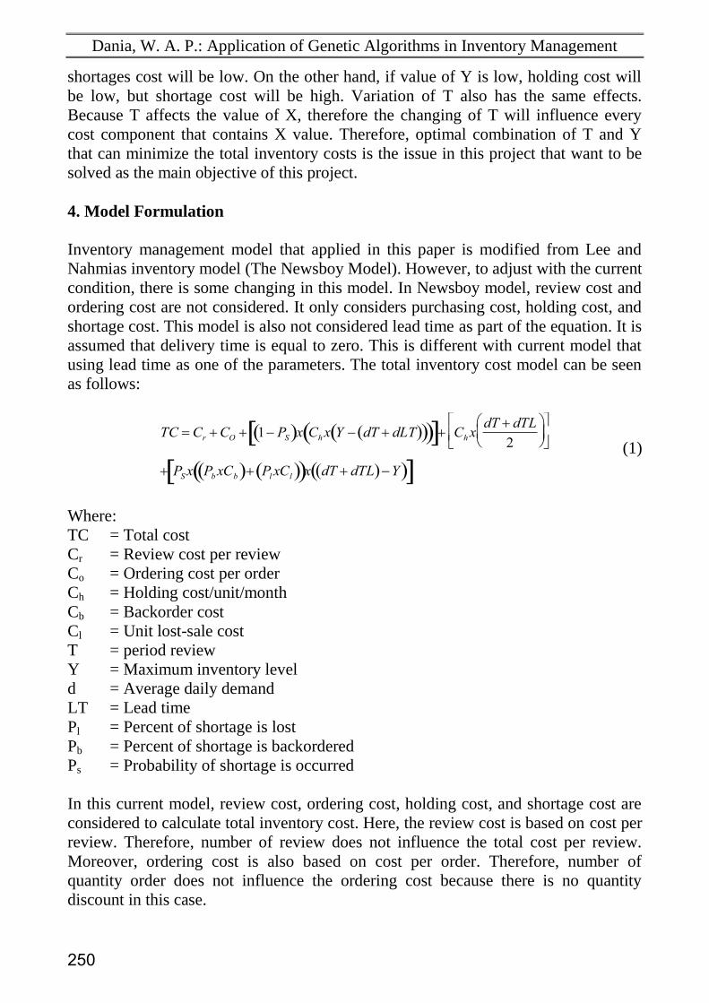
4. Model Formulation

Inventory management model that applied in this paper is modified from Lee and

Nahmias inventory model (The Newsboy Model). However, to adjust with the current

condition, there is some changing in this model. In Newsboy model, review cost and

ordering cost are not considered. It only considers purchasing cost, holding cost, and

shortage cost. This model is also not considered lead time as part of the equation. It is

assumed that delivery time is equal to zero. This is different with current model that

using lead time as one of the parameters. The total inventory cost model can be seen

as follows:

TC Cr CO 1 PS x Chx Y dT dLT ChxdT dTL

2

PSx PbxCb PlxCl x dT dTL Y (1)

Where:

TC = Total cost

Cr = Review cost per review

Co = Ordering cost per order

Ch = Holding cost/unit/month

Cb = Backorder cost

Cl = Unit lost-sale cost

T = period review

Y = Maximum inventory level

d = Average daily demand

LT = Lead time

Pl = Percent of shortage is lost

Pb = Percent of shortage is backordered

Ps = Probability of shortage is occurred

In this current model, review cost, ordering cost, holding cost, and shortage cost are

considered to calculate total inventory cost. Here, the review cost is based on cost per

review. Therefore, number of review does not influence the total cost per review.

Moreover, ordering cost is also based on cost per order. Therefore, number of

quantity order does not influence the ordering cost because there is no quantity

discount in this case.

250


Holding cost in this model is also different with holding cost in Newsboy model.

Because lead time is considered, demand during lead time is also calculated to get the

total of inventory that is carried. Extra stock will occur if total demand during period

is below the maximum inventory level. If extra stock occurs, there is no shortage

cost. Therefore, the probability of holding extra inventory is equal to 1 – Ps. Besides

hold the extra inventory, holding cost also occurs during the process. It includes the

average of inventory that is carried in one period before new order comes.

In addition, shortage cost is also considered in this model because the customer

demand is fluctuated. If shortage happens, it means that the customer demand above

the maximum inventory level. To calculate the shortage cost, the probability of

shortage is occurred also need to be determined. There are two conditions that might

be happened if shortage occurs. First, customers are willing to wait the delay,

therefore company needs to backorder the raw material. Second, customers do not

want to wait or company lost the sales. Therefore in this model, probability of

backorder and lost of sales are also considered.

5. Mechanism of the Proposed Genetic Algorithms

Conceptually, genetic algorithms as natural evolution optimization method use

biological term to represent the structure of model component. In population,

chromosomes represent individual components. Chromosomes consist of set of

structure which is called gene. Each gene will represent the potential solutions to

solve problems. Genetic algorithms will maximize the process of finding the optimal

solution from gene and chromosome by exploiting the available search space

(Michalewicz 1999).

From the mathematics model above, it is clear that the variables that want to be

optimized in this research are order interval (T) and maximum inventory level (Y). In

order to minimize the total inventory cost, the chromosome of the genetic algorithms

should include both T and Y. Because in this research chromosomes are represented

as integer number coding, therefore, chromosome only consists of two genes, which

each gene represents the real value of T and Y.

There are some combination among number of generation, population, crossover rate,

and mutation rate to find the optimal solution. Range for number generation is

between 150 and 300 which increase every 50 and range for number of population is

from 50 to 200 which increase every 50. Moreover, for crossover rate and mutation

rate, the range value is from 0.1 to 0.5 which increase every 0.1.All of the

combination is run by visual basic 6.0 to get the most optimal solution which has the

lowest total cost and best fitness.

5.1 Chromosome Population

After genes in chromosome are decided, the first step is generating random number

as the initial population. Total number of initial population will be generated as trial

and error. Here, numbers that are generated consist of two elements, T and Y.

However, when numbers are generated, it must consider the constraint of every

variable. Constraint of T is related to the maximum life cycle of the wheat flour in the

251


storage. While constraint of Y related to the minimum inventory level that must be

available in the storage. This level is related to lead time of the delivery order.

For order interval, the value cannot be higher than 30. It is because the life cycle of

wheat flour is maximum 30 days. In addition, related to inventory level, the minimum

of inventory level is 2,100 and the maximum inventory level is 25,000. The minimum

inventory level is decided based on the lead time of the delivery order and the

maximum inventory level is decided regarding the maximum life cycle of wheat

flour.

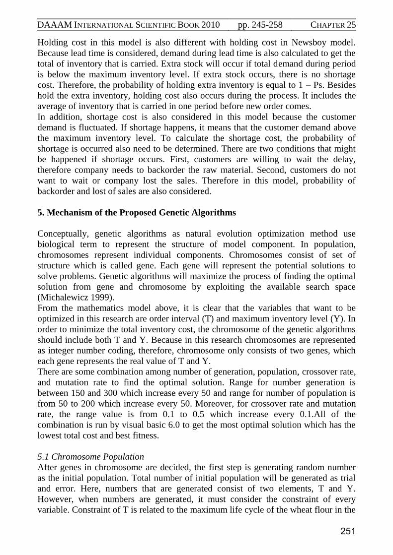
After the range of the variable is decided, the next step is coding process. Each value

of solution is coded to the integer number starting from 1. Therefore, the genetic

algorithms process does not work in the real value but in the coding value. For

variable T which has range from 2 to 30 days, coding is from 1 to 29. Therefore, code

1 represent 2 days, code 2 represents 3 days, and soon with the increment 1 unit.

However, for variable Y which has range from 2,100 to 25,000 bags, coding is from 1

to 22,901. Here, code 1 represents 2,100 bags, code 2 represents 2,101 bags, and soon

with the increment 1 unit. The example of initial population for this process can be

seen in Table 1.

T Y T Y T Y T Y T Y

4 17015 5 13506 21 16986 23 18053 7 22131

17 17034 22 17500 20 2188 11 9085 4 9490

11 13990 9 18197 15 8159 27 15867 19 18652

20 22585 25 15506 17 22785 25 17072 24 16133

24 15688 14 3439 25 3486 29 16120 14 22690

18 19996 3 22876 4 20188 9 15888 27 20215

25 15675 7 16011 17 7236 26 20069 5 9678

7 21055 28 2471 16 14920 16 4545 15 17175

23 17210 4 3085 28 14755 19 3429 12 6565

21 14303 8 16471 29 19409 29 7443 14 18695

Tab. 1. Population of Chromosomes

5.2 Selection Process for Current Model

After initial population is generated, current fitness value is evaluated and selected to

create new population for the next process. In this research, selection method that is

used is roulette wheel selection. Step by step of roulette wheel selection according to

Gen and Cheng (1997) that will be applied in this research are:

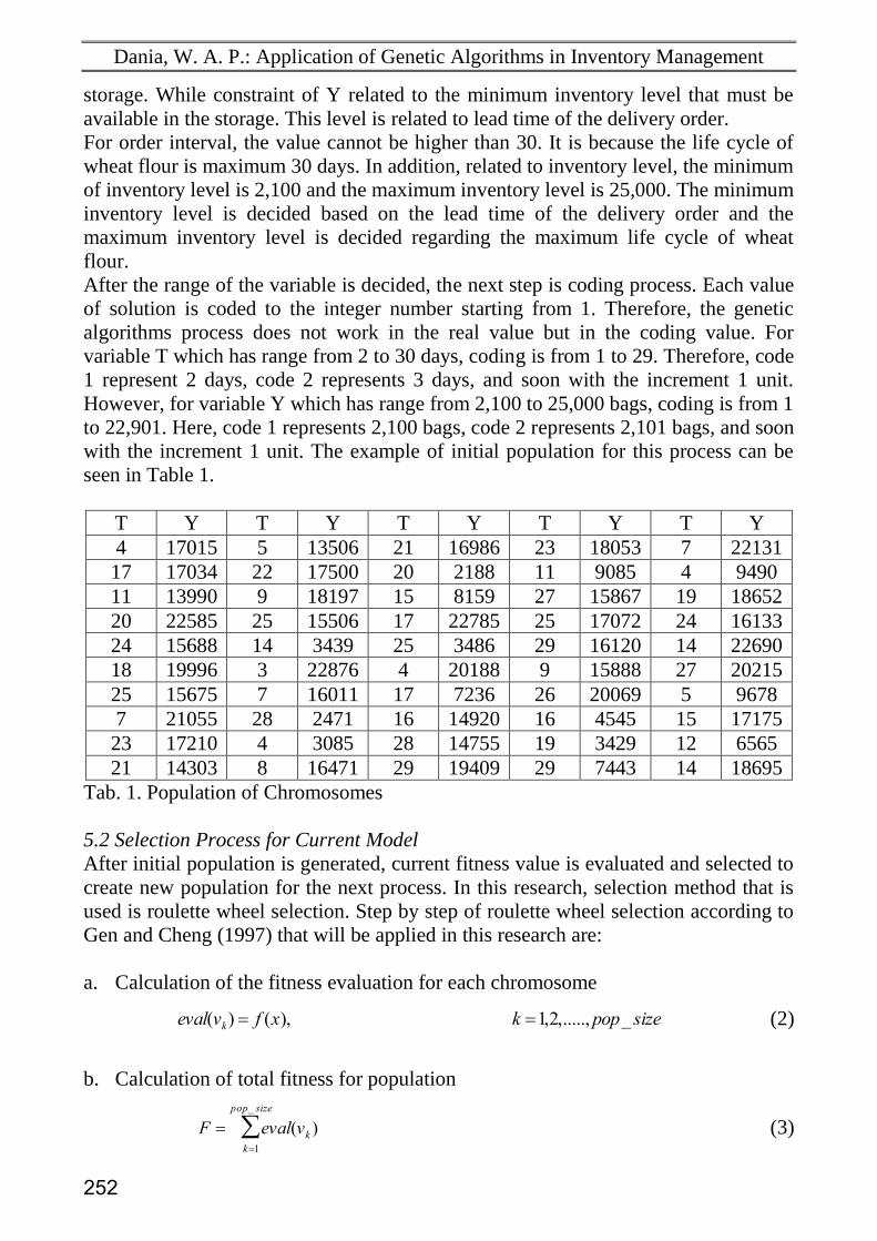
a. Calculation of the fitness evaluation for each chromosome

eval(vk) f (x),

k 1,2,.....,pop_ size (2)

b. Calculation of total fitness for population

F eval(vkk1

pop_ size

) (3)

252


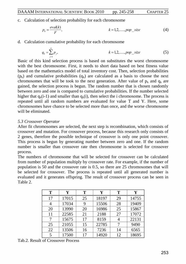
c. Calculation of selection probability for each chromosome

pk eval(k)

F,

k 1,2,.....,pop_ size (4)

d. Calculation cumulative probability for each chromosome

qk p j,j1

k

k 1,2,.....,pop_ size (5)

Basic of this kind selection process is based on substitutes the worst chromosome

with the best chromosome. First, it needs to short data based on best fitness value

based on the mathematics model of total inventory cost. Then, selection probabilities

(pk) and cumulative probabilities (qk) are calculated as a basis to choose the next

chromosomes that will be took to the next generation. After value of pk and qk are

gained, the selection process is begun. The random number that is chosen randomly

between zero and one is compared to cumulative probabilities. If the number selected

higher that qk(i-1) and smaller than qk(i), then select the i chromosome. The process is

repeated until all random numbers are evaluated for value T and Y. Here, some

chromosomes have chance to be selected more than once, and the worse chromosome

will be eliminated.

5.3 Crossover Operator

After fit chromosomes are selected, the next step is recombination, which consists of

crossover and mutation. For crossover process, because this research only consists of

2 genes, therefore the possible technique of crossover is only one point crossover.

This process is begun by generating number between zero and one. If the random

number is smaller than crossover rate then chromosome is selected for crossover

process.

The numbers of chromosome that will be selected for crossover can be calculated

from number of population multiply by crossover rate. For example, if the number of

population is 50 and the crossover rate is 0.5, so there are 25 chromosomes that will

be selected for crossover. The process is repeated until all generated number is

evaluated and it generates offspring. The result of crossover process can be seen in

Table 2.

T Y T Y T Y

17 17015 25 18197 29 14755

4 17034 9 15506 28 19409

20 13990 20 16986 25 15867

11 22585 21 2188 27 17072

7 15675 17 8159 4 22131

25 21055 15 22785 7 9490

22 13506 16 7236 14 6565

5 17500 17 14920 12 18695

Tab.2. Result of Crossover Process

253


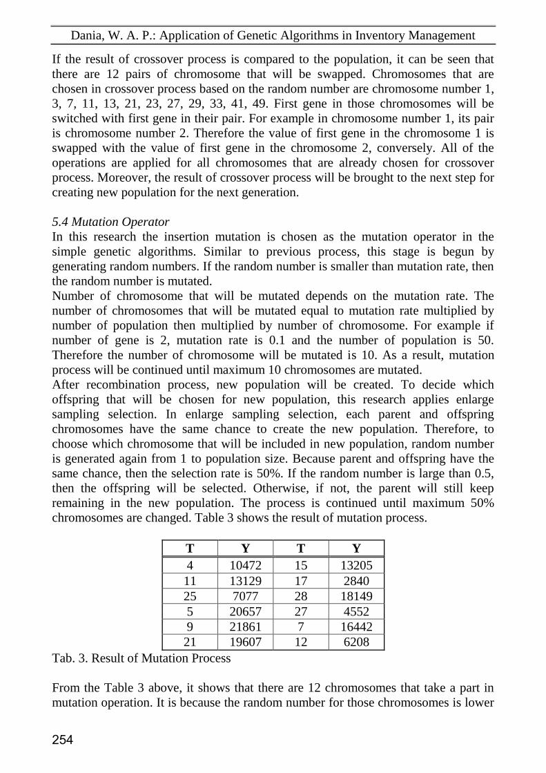
If the result of crossover process is compared to the population, it can be seen that

there are 12 pairs of chromosome that will be swapped. Chromosomes that are

chosen in crossover process based on the random number are chromosome number 1,

3, 7, 11, 13, 21, 23, 27, 29, 33, 41, 49. First gene in those chromosomes will be

switched with first gene in their pair. For example in chromosome number 1, its pair

is chromosome number 2. Therefore the value of first gene in the chromosome 1 is

swapped with the value of first gene in the chromosome 2, conversely. All of the

operations are applied for all chromosomes that are already chosen for crossover

process. Moreover, the result of crossover process will be brought to the next step for

creating new population for the next generation.

5.4 Mutation Operator

In this research the insertion mutation is chosen as the mutation operator in the

simple genetic algorithms. Similar to previous process, this stage is begun by

generating random numbers. If the random number is smaller than mutation rate, then

the random number is mutated.

Number of chromosome that will be mutated depends on the mutation rate. The

number of chromosomes that will be mutated equal to mutation rate multiplied by

number of population then multiplied by number of chromosome. For example if

number of gene is 2, mutation rate is 0.1 and the number of population is 50.

Therefore the number of chromosome will be mutated is 10. As a result, mutation

process will be continued until maximum 10 chromosomes are mutated.

After recombination process, new population will be created. To decide which

offspring that will be chosen for new population, this research applies enlarge

sampling selection. In enlarge sampling selection, each parent and offspring

chromosomes have the same chance to create the new population. Therefore, to

choose which chromosome that will be included in new population, random number

is generated again from 1 to population size. Because parent and offspring have the

same chance, then the selection rate is 50%. If the random number is large than 0.5,

then the offspring will be selected. Otherwise, if not, the parent will still keep

remaining in the new population. The process is continued until maximum 50%

chromosomes are changed. Table 3 shows the result of mutation process.

T Y T Y

4 10472 15 13205

11 13129 17 2840

25 7077 28 18149

5 20657 27 4552

9 21861 7 16442

21 19607 12 6208

Tab. 3. Result of Mutation Process

From the Table 3 above, it shows that there are 12 chromosomes that take a part in

mutation operation. It is because the random number for those chromosomes is lower

254


than mutation rate, which is 0.3. Number of chromosomes that are selected for

mutation process are 1, 3, 7, 11, 13, 21, 23, 27, 29, 22, 41, 49. In this process, the first

gene is fixed and the second gene is changed with the random number. For example,

in chromosome 6, value of T is the same with the initial population which is 21.

However, the value of Y is changed to 19,607. This operation is repeated until all the

chromosomes that are selected for mutation is processed.

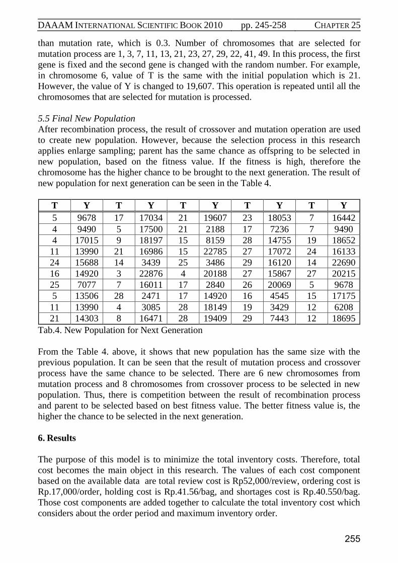
5.5 Final New Population

After recombination process, the result of crossover and mutation operation are used

to create new population. However, because the selection process in this research

applies enlarge sampling; parent has the same chance as offspring to be selected in

new population, based on the fitness value. If the fitness is high, therefore the

chromosome has the higher chance to be brought to the next generation. The result of

new population for next generation can be seen in the Table 4.

T Y T Y T Y T Y T Y

5 9678 17 17034 21 19607 23 18053 7 16442

4 9490 5 17500 21 2188 17 7236 7 9490

4 17015 9 18197 15 8159 28 14755 19 18652

11 13990 21 16986 15 22785 27 17072 24 16133

24 15688 14 3439 25 3486 29 16120 14 22690

16 14920 3 22876 4 20188 27 15867 27 20215

25 7077 7 16011 17 2840 26 20069 5 9678

5 13506 28 2471 17 14920 16 4545 15 17175

11 13990 4 3085 28 18149 19 3429 12 6208

21 14303 8 16471 28 19409 29 7443 12 18695

Tab.4. New Population for Next Generation

From the Table 4. above, it shows that new population has the same size with the

previous population. It can be seen that the result of mutation process and crossover

process have the same chance to be selected. There are 6 new chromosomes from

mutation process and 8 chromosomes from crossover process to be selected in new

population. Thus, there is competition between the result of recombination process

and parent to be selected based on best fitness value. The better fitness value is, the

higher the chance to be selected in the next generation.

6. Results

The purpose of this model is to minimize the total inventory costs. Therefore, total

cost becomes the main object in this research. The values of each cost component

based on the available data are total review cost is Rp52,000/review, ordering cost is

Rp.17,000/order, holding cost is Rp.41.56/bag, and shortages cost is Rp.40.550/bag.

Those cost components are added together to calculate the total inventory cost which

considers about the order period and maximum inventory order.

255


From the result of all combination of four parameter (generation, population,

crossover rate, and mutation rate), the minimum total cost which indicates the best

fitness value is found in combination of 300 generations, 200 population size, 0.4

crossover rate, and 0.2 mutation rate. This combination gives the result of variable T

equal to 1 and Y equal to 1,005. This result gives the optimal solution from global

optima. It can be seen from the graph that the average fitness value increase along the

generation and minimize the range between worse fitness, average fitness, and best

fitness. Graphic that shows about the increasing of fitness value in the best

combination for this case can be seen at Figure 1.

Fig. 1. Graphic of Search Process (Combination of 200 Population Size, 300

Generation, 0.4 Crossover Rate, and 0.2 Mutation Rate)

After getting the result, the next process is decoding process to get the real value of

the optimal result. The purpose of decoding process is to convert the chromosome of

genetic algorithms from coding space into solution space. After decoding, the value

of T and Y becomes 2 and 3,104 respectively. This result bring total cost to the

minimum point which is Rp.133,517.02.

Before applying genetic algorithms in the inventory system, this company already has

its current system. In its system, raw material is ordered every 3 days and the quantity

order is 2,292 bags each delivery. This system does not apply buffer stock. As a

result, it assumes that in every period, the inventory level goes down to zero and after

receiving order the quantity of order brings the inventory level up to the maximum

level. From this company’s inventory system, using those data as an input to calculate

the total inventory cost, total cost per review becomes Rp.29,961,629.2. By reducing

the order period from 3 days to 2 days and increasing the maximum inventory level

from 2,292 bags to 3,104 bags, this approach gives benefit to the company up to

99.55% reduction from the total inventory cost per review or 93.32% per 6 month.

1

2

3

1

2

3

256


This value brings big impact in term of benefit for the company. The small change of

the variables in the system (T and Y) gives the significant impact to the company’s

environment in global.

7. Conclusion and Future Research

This research is presented to develop the inventory model using periodic review

model to solve the inventory problem in UWBM Company as a case study to

minimize the total inventory cost. This research designed inventory management

system related to the optimal order review period and maximum inventory level. To

solve this problem, genetic algorithms approach is used to find the optimal solution

which brings the total inventory cost to the minimal point.

After genetic algorithms are generated, the optimal solution for this company is

found. The most optimal combination to find the optimal solution is from

combination of 300 generations, 200 populations, 0.4 crossover rates, and 0.2

mutation rates. The optimal results of this case study are 2 days review period and

3,104 maximum inventory level which gives the minimum total inventory cost is

Rp.133,517.02. This result gives cost efficiency compared to current company

inventory system up to 99.55% per review or 93.32% per 6 month.

Although this research result gives high efficiency to the reduction of total cost, there

are limitation related to the inventory model and genetic algorithms. These

limitations are:

The mathematics model that is developed in this research did not consider the

safety stock in the system. It is assumed that all the raw materials can handle the

customer order.

Related to genetic algorithms, type of genetic algorithms that are applied in this

research is simple GAs that using integer number not a binary number. Therefore,

each chromosome only consists of 2 genes.

The inventory model that is developed in this research only solves the problem in

UWBM Company, especially for wheat flour. Therefore, the optimal solution is

only valid for this specific company and specific product.

To improve the study in this topic, there are future works that can be considered to be

the next research areas such as:

Developing the mathematics model that considers any aspects those are not

implemented in this current model, such as safety stock, unknown lead time,

quantity discount, and so on.

Developing more complicated and comprehensive genetic algorithms by using

binary number and others crossover and mutation methods.

Improving the crossover rate and mutation rate with more combination of

generation and population.

Extending this model, not only considering for 1 type of raw material but also for

all raw materials from one supplier (PT. ISM Bogasari Flour Mills Surabaya)

Using sensitivity analysis to analyze the robustness of the result for several

condition

257


8. References

Chiang, C. (2009). ‘A periodic review replenishment model with a refined delivery

scenario’, International Journal of Production Economics, vol. 118, (2008),

pp. 253-259, 0925-5273

Chong, E. K. P. & Zak, S. H. (1996).An Introduction to Optimization, Wiley-

Interscience, 0471089494, New York

Chopra, S. & Meindl, P. (2007).Supply Chain Management: Strategy, Planning, and

Operation, Pearson Prentice-Hall Publishers, 0131730428, New York

Chuang, B.R; Ouyang, L.Y & Chuang K.W. (2004). ‘A note on periodic review

inventory model with controllable setup cost and lead time’, Computers &

Operations Research, vol.31, (2003), pp. 549-561, 0305-0548

Davis, L. (1996).Handbook of Genetic Algorithms, International Thomson Computer

Press, 1850328250, Boston

Flynn, J. & Garstka, S. (1997). ‘The optimal review period in a dynamic inventory

model’, Journal of Operations Research, vol.45, (September-October 1997),

pp. 736-750, 0030-364x

Gen, M. & Cheng, R. (1997).Genetic Algorithms & Engineering Design, John Willey

& Sons, Inc, 0471127418, New York

Goldberg, D. E. (1989).Genetic algorithms, In search, Optimisation & Machine

Learning, Addison-Wesley Publishing Company, Inc, 0201157675,

Massachusetts

Haupt, R. L. & Haupt, S. E. (1998).Practical Genetic Algorithms, John Willey &

Sons, Inc, 0471188735, New York

Heizer, J. H. & Render, B. (1993).Production and Operation Management:

Strategies and Tactics, Allyn and Bacon, 0205140483, Boston

Hill, T. (2005).Operations Management, Palgrave Macmillan, 140399112X,

Hampshire

Hou, C.I.; Lo, C.Y & Leu, J.H.(2007). Use genetic algorithm in production and

inventory strategy, Proceedings of the 2007 IEEE IEEM, pp. 963-967, 1-4244-

1529-2

Maiti, A.K.; Bhunia, A.K. &Maiti, M.(2006). ‘An application of real-coded genetic

algorithm (RCGA) for mixed integer non-linear programming in two storage

multi-item inventory model with discount policy’, Applied Mathematics and

Computation, vol.183, (2006), pp. 903-915, 0096-3003

Michalewicz, Z. 1999, Genetic Algorithms + Data Structures = Evolution Programs,

Springer-Verlag, 3540606769, Berlin.

Starr, M. K. (2007).Foundations of Production & Operations Management,

Thomson, 1592602762,USA

Stock, J. R. & Lambert, D. M. (2001).Strategic Logistics Management, McGraw-Hill

Higher Education, 0256136874, Boston

Stockton, D. J. & Quinn, L. (1993). ‘Identifying economic order quantities using

genetic algorithms’, International Journal of Operation & Production

Management, vol.13, (1993), pp. 92-103, 0144-3577

258

Documents

DAAAM INTERNATIONAL SCIENTIFIC BOOK 2010 pp. · PDF fileApplication of Genetic Algorithms in Inventory Management, ... establish the basic EOQ model using Genetic Algorithms ... GAs