1

(D37) INFORMATIK I October 4 2007 (Moritz Winger) 6 Polymer Reptation Monte Carlo Simulation Contents Page 1 Introduction 2 2 Background 2 2.1 Simulation 3 2.2 Determining average properties 3 2.3 Periodic boundary conditions [1 question] 6 3 The “polyrep” program 7 3.1 Finding and running the program 7 3.2 Program structure [3 questions] 8 3.3 Walking through the main program (the function main) [4 questions] 8 3.4 Input you must give to the program 9 3.5 Testing the program [3 exercises] 10 4 Programming exercises 10

A. Determining the x- and y-components of the root mean-square head-to-tail distance of a polymer chain 12

B. Calculating the root mean-square radius of gyration of a polymer chain 13 C. Calculating a histogram of head-to-tail distances of a polymer chain 15 5 References 17 6 Appendices A. Input file format for the program “polyrep” 18 B. Listing of input files 18 C. Listing of the program text “polyrep.cc” 19

2

Exercise 6 Polymer Reptation Monte Carlo 1 Introduction As a scientist using computer programs, you often confront programs that do almost, but not exactly, what you would like them to do. You can then either write a new program, or modify the program you have. In this practical you will modify a long program, which does computer simulation. It simulates polymer geometries with the reptation Monte Carlo method. The simulation program is written in C++, so you should know a little of this language. You will run test calculations to get to know the program. You will then modify the program to analyze the simulations in new ways. For every “Question” or “Exercise” in these instructions, you have to give answers in your short written report. Questions can be done in advance, for Exercises you need a computer. In paragraph 4 you choose one of the Programming Exercises A, B and C. Your report should be mailed to ex6@igc.phys.chem.ethz.ch. Also make a printout and put it in the appropriate mailbox in room HCI G 238. The report should be written (preferably) in English. 2 Background The word “polymers” is used for many kinds of molecules, from complex, information-rich polypeptides and polynucleotides of living organisms to simple, repetitive chains in important materials like plastics, rubber and cellulose. All polymers are chains of monomeric units, typically 102-104 units. A polymer is described chemically by its monomeric unit(s), e.g. polyisoprene (rubber) is {-CH2-C(CH3)=CH-CH2-}n. Any single chain has a definite value of n (the number of monomeric units) while in the bulk system, like a drop of polymer solution or a piece of polymeric material, n takes on a range of values depending on how the polymer was synthesized. Proteins and nucleic acids are special cases, since they are made in the cell to have an exact information content and chain length. Even so, protein solutions may show length variations like synthetic polymer solutions, if they contain many different proteins. In a polymer solution or a polymeric material, every polymer molecule has a different geometry. Long chains have many possible conformations; for example, a chain consisting of n bonds each with three low-energy rotational possibilities can adopt 3n (~10n/2) conformations. This is a very large number if n is maybe 1000. The size and shape of the molecules change during time, as they twist, bend and turn when they interact with themselves and with other polymer molecules and solvent molecules. Properties of bulk polymers are average properties, that depend on which are common and which are rare among these conformations of individual molecules. Therefore statistical techniques are used (Flory, 1969). One can learn things that are valid for all polymers by ignoring chemical details and calculating statistical results from general polymer models. In this practical we meet a very general type of polymer models, the lattice models, in which a flexible polymer chain of N monomeric units is represented as (N-1) little “steps”, one step for each link between monomeric units in the polymer. These steps do not walk around just anyhow, but each step has to land on a “lattice point”, which is a possible position for a monomeric unit. The points are arranged in some periodic pattern in space,

3

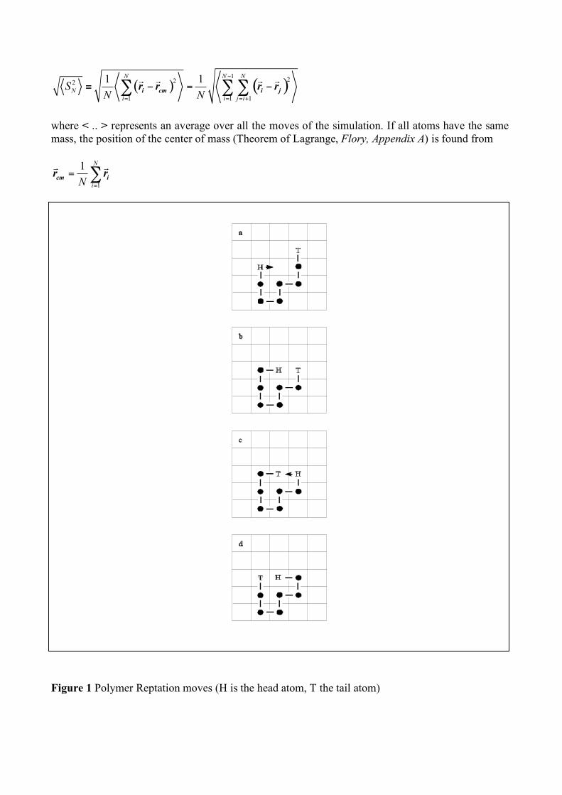
and a walk cannot visit the same point more than once - only one monomeric unit can fit on a lattice point. There is a choice for each step from nearby lattice points to go to, and the result of all these choices is the conformation of the molecule. In a simple model, this is a random choice. So our model polymer molecule is a self-avoiding random walk on a periodic lattice. The lattice can have 1,2,3 or more dimensions, and may be triangular, square, tetrahedral, cubic or any other periodic geometry. 2.1 Simulation Studying self-avoiding random walks analytically with pen and paper is difficult, but the models are suitable for computer simulation (Baumgärtner, 1987; Lowry, 1976). Even computer investigations usually focus on short chains, for which the results are almost exact, and extrapolate to longer chains. The idea with computer simulations is to not look at every possible conformation, but to generate a representative set of conformations with the same average properties as the set of all conformations. Many generation methods are based on “moves”, where the result after a move is a new conformation, which is counted for statistics and used as the starting point for the next move. Here we move according to the reptation method (Wall and Mandel, 1975), which is good for linear chains. Our polymer consists of monomeric units - let us call them “atoms”- and sits on a lattice (Figure 1). The head atom moves to a randomly chosen nearby position with the rest of the chain following like a 'slithering snake' - a motion called reptation. This means selecting a new head position and deleting the tail atom at the other end of the chain. If the selected new head position is occupied by another atom the move is rejected, otherwise it is accepted. Either end of the chain can be chosen as the head, reducing the problem of the chain becoming stuck with its head buried in a cul-de-sac. Every conformation generated is used in the averaging procedures, and when a move attempt fails the conformation is recounted. Because of the random decision of to where a trial move is attempted, this procedure is termed polymer reptation Monte Carlo (M. C. is well-known for random events studies). Consider, for example, a single polymer chain of 8 atoms on a two-dimensional square lattice (Figure 1). A trial move of the head atom is indicated by the arrow. In this case the new head site is vacant, the move is accepted, so conformation (b) is generated. This time the same head atom is chosen again, but the proposed downward move would lead to a clash of atoms and so the move is rejected. The same conformation is therefore kept in (c). Now the head and tail are switched as a result of a random choice. The next move is accepted since the new head position will have been vacated by the tail atom after the move, giving conformation (d). The process is repeated over and over. 2.2 Determining Average Properties We measure the size of a polymer chain with two numbers: the root-mean-square head-to-tail distance and the root-mean-square radius of gyration. Root-mean-square head-to-tail distance is

( ) ( )2

122

1 1

1

N j jr r r r!

=

" #$ ! = !% &

' ()

r r r rN

N

j

R +

where rjr is the position vector of atom j in a N atom chain. Root-mean-square radius of gyration is

4

( ) ( )1

222

1 1 1

1 1

i cm i jr r r r!

= = = +

" ! = !# # #r r r r

N N N

N

i i j i

SN N

where < .. > represents an average over all the moves of the simulation. If all atoms have the same mass, the position of the center of mass (Theorem of Lagrange, Flory, Appendix A) is found from

1

1

cm ir r

=

= !r r

N

iN

Figure 1 Polymer Reptation moves (H is the head atom, T the tail atom)

5

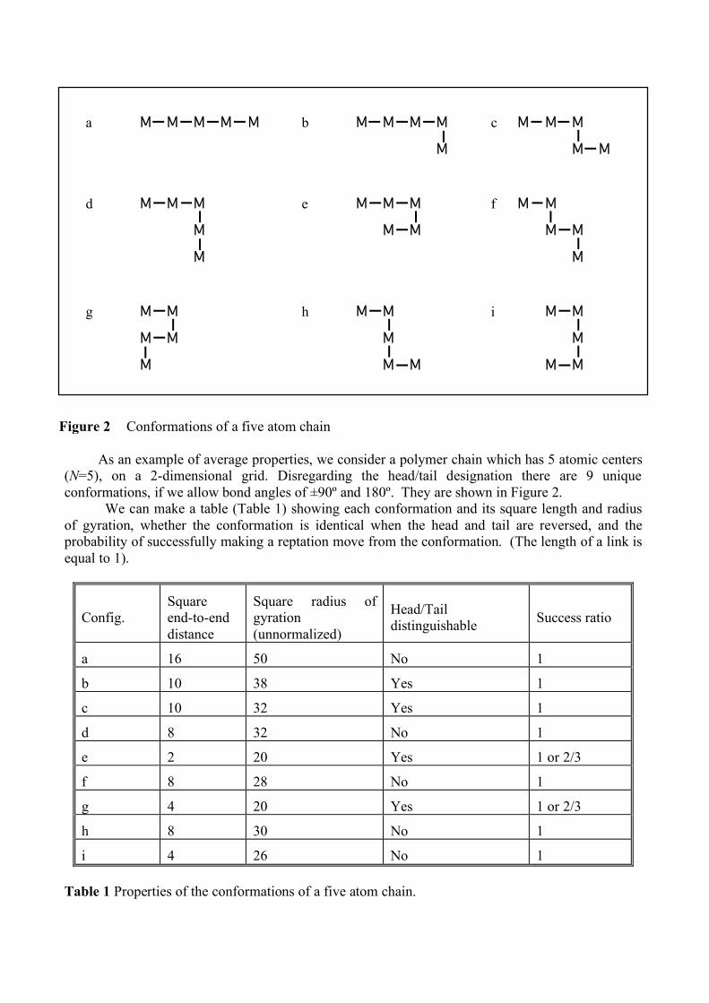
As an example of average properties, we consider a polymer chain which has 5 atomic centers (N=5), on a 2-dimensional grid. Disregarding the head/tail designation there are 9 unique conformations, if we allow bond angles of ±90º and 180º. They are shown in Figure 2. We can make a table (Table 1) showing each conformation and its square length and radius of gyration, whether the conformation is identical when the head and tail are reversed, and the probability of successfully making a reptation move from the conformation. (The length of a link is equal to 1).

Config. Square end-to-end distance

Square radius of gyration (unnormalized)

Head/Tail distinguishable Success ratio

a 16 50 No 1

b 10 38 Yes 1

c 10 32 Yes 1

d 8 32 No 1

e 2 20 Yes 1 or 2/3

f 8 28 No 1

g 4 20 Yes 1 or 2/3

h 8 30 No 1

i 4 26 No 1 Table 1 Properties of the conformations of a five atom chain.

Figure 2 Conformations of a five atom chain

a

d

g

MM M M M

M M M

M

M

M M

MM

M

bM M M M

M

e M M M M

M

h M M

M

M M

c M M M

M M

f

M

M

M M

M

i M M

M

MM

6

Forming averages of the root-mean-square head-to-tail distance is not so simple. For example, conformation (a) can occur in 2 different ways for any given starting point, while conformation (b) can occur in 8 different ways. Furthermore, each of the conformations of (b) is distinguishable from one in which the head/tail designation is reversed, whereas the head/tail designation makes no difference for conformation (a). Thus conformation (b) will occur 4 times as often as conformation (a). We need to weigh the contribution of each conformation to the average value of the squared head-to-tail distance accordingly. Counting conformations the same way, we get relative weights 1,4,4,2,4,2,4,2 and 2 for conformations (a) to (i) respectively. The root-mean-square head-to-tail distance becomes

2 1 16 4 10 4 10 2 8 4 2 2 8 4 4 2 8 2 4

1 4 4 2 4 2 4 2 2

2.65

NR

! + ! + ! + ! + ! + ! + ! + ! + !=

+ + + + + + + +

=

We may calculate the expected acceptance ratio for our polymer simulation in the same way, from the weights of each conformation and their individual acceptance ratios. For example, in conformation (a) any attempted move will be successful, irrespective of which end of the polymer is the head.

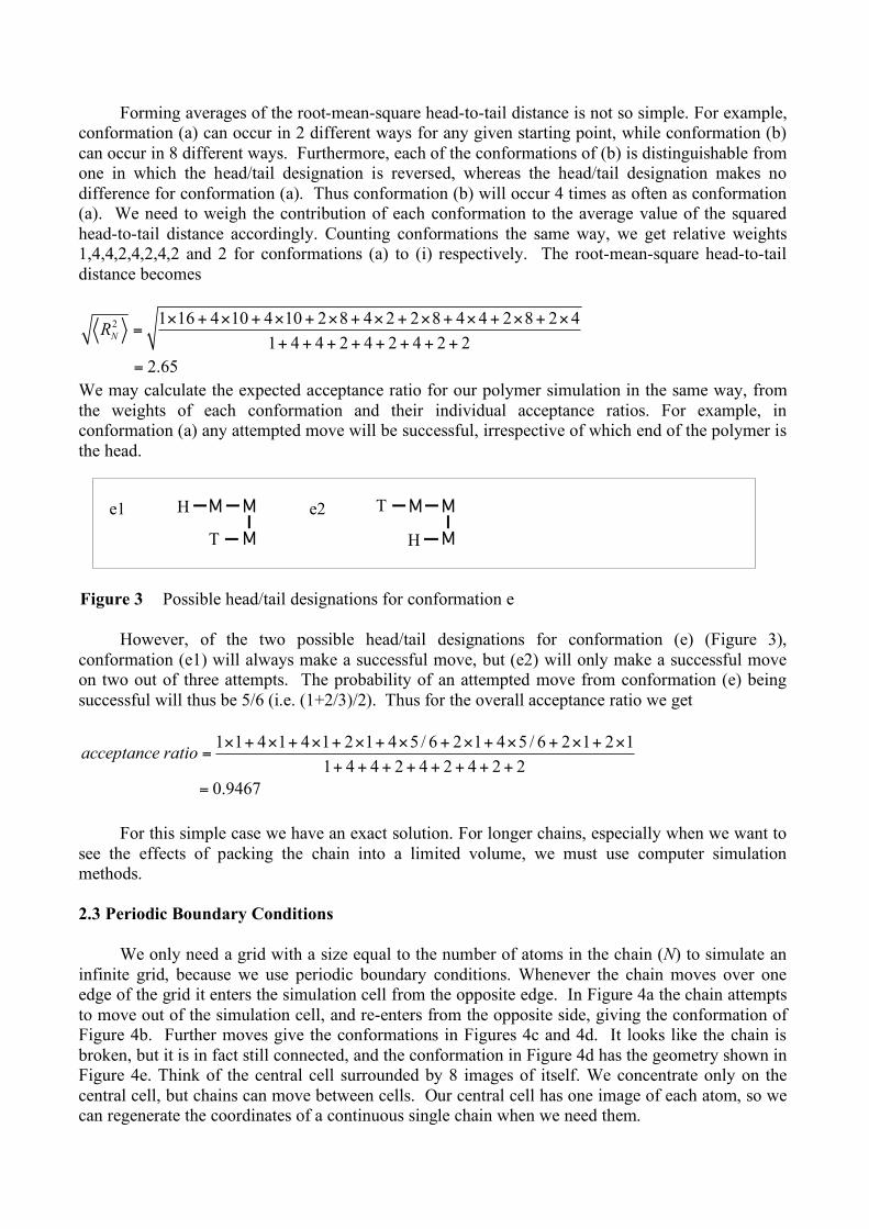
However, of the two possible head/tail designations for conformation (e) (Figure 3), conformation (e1) will always make a successful move, but (e2) will only make a successful move on two out of three attempts. The probability of an attempted move from conformation (e) being successful will thus be 5/6 (i.e. (1+2/3)/2). Thus for the overall acceptance ratio we get

1 1 4 1 4 1 2 1 4 5 / 6 2 1 4 5 / 6 2 1 2 1

1 4 4 2 4 2 4 2 2

0.9467

acceptance ratio! + ! + ! + ! + ! + ! + ! + ! + !

=+ + + + + + + +

=

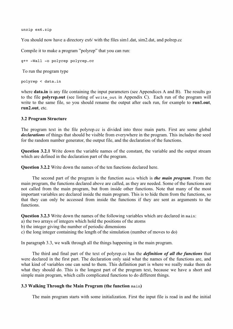
For this simple case we have an exact solution. For longer chains, especially when we want to see the effects of packing the chain into a limited volume, we must use computer simulation methods. 2.3 Periodic Boundary Conditions We only need a grid with a size equal to the number of atoms in the chain (N) to simulate an infinite grid, because we use periodic boundary conditions. Whenever the chain moves over one edge of the grid it enters the simulation cell from the opposite edge. In Figure 4a the chain attempts to move out of the simulation cell, and re-enters from the opposite side, giving the conformation of Figure 4b. Further moves give the conformations in Figures 4c and 4d. It looks like the chain is broken, but it is in fact still connected, and the conformation in Figure 4d has the geometry shown in Figure 4e. Think of the central cell surrounded by 8 images of itself. We concentrate only on the central cell, but chains can move between cells. Our central cell has one image of each atom, so we can regenerate the coordinates of a continuous single chain when we need them.

Figure 3 Possible head/tail designations for conformation e

M M

M

H

T

M M

M

T

H

e1 e2

7

Question 2.3.1 Draw these 9 cells, and put in the polymer (all 9 copies) in the conformation of 4d. 3 The “polyrep” Program The polyrep program performs a simple polymer reptation Monte Carlo scheme in two dimensions. It has periodicity in 0, 1, or 2 dimensions (sizes of restricted dimensions are specified by the user). The following sections describe the program. The program text is listed in Appendix C. 3.1 Finding and Running the Program

All files for this exercise are located on the webpage www.igc.ethz.ch/education/Basic/exe/MC. Download the linked zip file and unzip it by typing:

Figure 4 Illustrating periodic boundary conditions

M M M MT

H

a

H

b

MM

M

T

MM M M TT

H

d

M

H

c

M M TM M T

HM

e

8

unzip ex6.zip You should now have a directory ex6/ with the files sim1.dat, sim2.dat, and polrep.cc

Compile it to make a program ”polyrep” that you can run: g++ -Wall -o polyrep polyrep.cc To run the program type polyrep < data.in where data.in is any file containing the input parameters (see Appendices A and B). The results go to the file polyrep.out (see listing of write_out in Appendix C). Each run of the program will write to the same file, so you should rename the output after each run, for example to run1.out, run2.out, etc. 3.2 Program Structure The program text in the file polyrep.cc is divided into three main parts. First are some global declarations of things that should be visible from everywhere in the program. This includes the seed for the random number generator, the output file, and the declaration of the functions. Question 3.2.1 Write down the variable names of the constant, the variable and the output stream which are defined in the declaration part of the program. Question 3.2.2 Write down the names of the ten functions declared here. The second part of the program is the function main which is the main program. From the main program, the functions declared above are called, as they are needed. Some of the functions are not called from the main program, but from inside other functions. Note that many of the most important variables are declared inside the main program. This is to hide them from the functions, so that they can only be accessed from inside the functions if they are sent as arguments to the functions. Question 3.2.3 Write down the names of the following variables which are declared in main: a) the two arrays of integers which hold the positions of the atoms b) the integer giving the number of periodic dimensions c) the long integer containing the length of the simulation (number of moves to do) In paragraph 3.3, we walk through all the things happening in the main program. The third and final part of the text of polyrep.cc has the definition of all the functions that were declared in the first part. The declaration only said what the names of the functions are, and what kind of variables one can send to them. This definition part is where we really make them do what they should do. This is the longest part of the program text, because we have a short and simple main program, which calls complicated functions to do different things. 3.3 Walking Through the Main Program (the function main) The main program starts with some initialization. First the input file is read in and the initial

9

polymer conformation is generated. These two things happen when the function read_in is called. Then the function draw_grid is called, to write a picture of the initial conformation to the output file. After that, some variables are initialized to zero. These variables are where the statistics from the simulation are going to be stored. Then comes the real Monte Carlo loop. It is a for loop which uses the variable attempt to count how many move attempts have been done so far. Question 3.3.1 What is the initial value of attempt? What comparison is made to see if we have to make more move attempts? Every time the Monte Carlo loop is performed, the following things happen: First the function swap_head is called to make a random decision about which end of the chain is going to be the head end for this move attempt. If a decision was taken to use the other end as the head compared to last time, the counter variable for head swaps (a statistics variable) is increased by one. Question 3.3.2 What is the name of the variable which counts head swaps? Then, a random move is attempted, by calling the function make_move. If the move was successful, the counter for successful moves (a statistics variable) is increased by one. Finally, the square of the head-to-tail distance is computed by the function get_len2, and this value is added to the third of the statistics variables. Question 3.3.3 What is the name of this third statistics variable? Now, the Monte Carlo loop ends. The loop is run again and again, every time increasing the variable attempt, until the comparison mentioned in Question 3.3.1 no longer gives the value TRUE. After running all the Monte Carlo move attempts, the final results are calculated. First, the root-mean-square head-to-tail distance is computed by calculating the mean value of the squares that have been summed during the Monte Carlo loops (in the third of the statistics variables), and taking the square root of that. Second, the success rate is calculated, as the number of successes divided by the number of attempts. These results are written as a line of results on the screen. This is one place where you will probably want to change the program, so you get some other results written on the screen! Question 3.3.4 Values of which three variables are written to the screen here in the original version of the polyrep program? After writing a line on the screen, a picture of the final conformation is written to the output file, by a new call to the function draw_grid. And finally the results are written to the output file, when the function write_out is called, and the output file is closed. 3.4 Input You Must Give to the Program The input options to the program are described in Appendix A. Put them in a file, like those listed in Appendix B, so you can use them again and make some changes and use them again... Choose a title that describes the calculation being performed, so you can recognize it easily afterwards. You must give a seed for the random number generator, the size of the polymer chain, and the length of the simulation. You can give one out of three values to the number of periodic dimensions in the simulation:

10

(a) 2 periodic dimensions. The polymer chain will move on the lattice as if the lattice is infinite

in both the x and the y directions. This is done with the periodic boundary conditions of section 2.3.

(b) 1 periodic dimension. The system is periodic in the x direction, so the chain is free to move

infinitely far. In the y direction, however, walls on the edge of the lattice keep the chain restricted. Therefore, you must give the size of the lattice in the y direction.

(c) 0 periodic dimensions. Walls are placed on all four sides of the lattice, confining the chain.

Therefore, you must give both the sizes of the lattice: in the x direction and in the y direction. 3.5 Testing the program Exercise 3.5.1 Convergence of Properties For reliable averages we need a statistically representative sample of polymer conformations. To see how many simulation steps this requires, simulate an 11 atom chain on a grid that is periodic in two dimensions (see file sim1.dat in Appendix C). Run for 100, 1000, 5000, 10000, 20000, 40000, 60000, 80000 and 100000 steps (change the NTimes parameter). Does the head to tail distance converge? Exercise 3.5.2 CPU Time and Root Mean-Square Head-to-Tail Distance as a Function of Chain Length To determine the amount of CPU time a program needs you can use the UNIX command time. The syntax for using time is: time polyrep < data.in time prints a line of which we only need the first number: the time in seconds that the CPU spent in the program. See how the CPU time required varies with the length of the chain. Start with a 3 atom chain (see file sim2.dat in Appendix B) and increase the chain length (parameter Natom) in successive simulations by 4 up to a length of 31. Find also relationships between the root mean-square head-to-tail distance and the number of atoms in the chain, and between the acceptance ratio and the number of atoms. Exercise 3.5.3 Comparison of Simulation and Theory Compare a simulation with the theoretical results for a 5 atom chain in section 2.2. Simulate NTimes=50000 steps with 2-dimensional periodicity (NPer=2). Do simulation and theory agree? 4 Programming Exercises In all three exercises you determine some form of relationship, so you should make plots (using the xmgrace program) to visualize your results. Choose one of the following programming exercises (A, B or C) and add to the report where you have already answered the questions above!

11

Include the following in your report: (a) A list of the changes you have made to the original program. If my_prog.cc is your own copy of the polyrep.cc program with your changes, you can produce a file my_changes.diff containing a list of the differences between the two programs, by diff polyrep.cc my_prog.cc > my_changes.diff (b) Any graphs that are required, suitably titled and labeled. (c) Written answers to all “Questions” and “Exercises” that are given in 2.3, 3.2, 3.3 and 3.5. Begin your report with your name, your user-name (e.g. >einstein'), and the date. Also, write the name and location of your program, so that it can be checked. If you work together with someone, this MUST be stated on the report and in the comments of the program.

12

Exercise A Determining the x- and y-components of the root-mean-square head-to-tail distance of a polymer chain The polyrep program calculates the total root-mean-square head-to-tail distance of a polymer chain, but often it would be interesting to know the x- and y-component of the root-mean-square head-to-tail distance, especially to know what happens to the shape of the polymer chain when there are changes in the environment. Modify the polyrep program so that it outputs both the x- and y-components of the root-mean-square head-to-tail distance. The squared lengths needed are already calculated in the function get_len2 (variables distX2 and distY2), but you will have to: (1) Pass the variables back to the main loop of the program and accumulate their values. (2) Average their values and compute the root once all the steps of the simulation have been

performed. (3) Include their values in the parameter list of the procedure write_out so that they are

written to the output file. (4) Write their values for plotting. This can be done by putting output statements writing to

the standard output stream (“the screen”), at the place in the program where the original program outputs three values. A good new set of output statements could be

cout << latsizY << " "; cout << XRMSL << " "; cout << YRMSL << " "; cout << RMSL << endl;

where latsizY is the thickness of the layer, RMSL is the root-mean-square head-to-tail

distance calculated during the simulation, and XRMSL and YRMSL are the x- and y-components of the root-mean-square head-to-tail distance that you have changed the program to calculate.

If your compiled modified program is called polyrep1, then you should run it using the command: polyrep1 < data.in >> plot.dat As before it will take the input from the file data.in, but the data for plotting will be appended to the file plot.dat. Each run of your modified program will add an extra line to the plot.dat file, and when you have finished your runs this file will be ready to be read into xmgrace for plotting a graph. Use your modified program to study the effect of the width of the lattice on the root-mean-square head-to-tail distance of a 11 atom polymer chain. Make the system periodic in the x-dimension (NPer=1) and, in separate runs, restrict the size of the y-dimension (LatY) to 2,3,4,..,10,20,30 and 40 layers respectively. Each run should make NTimes=10000 trial moves. Plot the root-mean-square head-to-tail distance and its x- and y-components as a function of the layer thickness (LatY), on the same graph. Do the various head-to-tail distances behave as you would expect? What do you think will happen to them as the thickness of the layer is increased further? In your written report include the answers to these questions, a plot of your graph (suitably titled and labeled) and a printout of the changes you have made to the program.

13

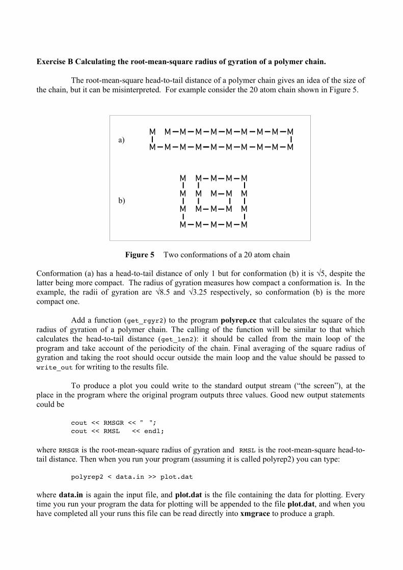
Exercise B Calculating the root-mean-square radius of gyration of a polymer chain. The root-mean-square head-to-tail distance of a polymer chain gives an idea of the size of the chain, but it can be misinterpreted. For example consider the 20 atom chain shown in Figure 5.

Conformation (a) has a head-to-tail distance of only 1 but for conformation (b) it is √5, despite the latter being more compact. The radius of gyration measures how compact a conformation is. In the example, the radii of gyration are √8.5 and √3.25 respectively, so conformation (b) is the more compact one. Add a function (get_rgyr2) to the program polyrep.cc that calculates the square of the radius of gyration of a polymer chain. The calling of the function will be similar to that which calculates the head-to-tail distance (get_len2): it should be called from the main loop of the program and take account of the periodicity of the chain. Final averaging of the square radius of gyration and taking the root should occur outside the main loop and the value should be passed to write_out for writing to the results file. To produce a plot you could write to the standard output stream (“the screen”), at the place in the program where the original program outputs three values. Good new output statements could be cout << RMSGR << " "; cout << RMSL << endl;

where RMSGR is the root-mean-square radius of gyration and RMSL is the root-mean-square head-to-tail distance. Then when you run your program (assuming it is called polyrep2) you can type: polyrep2 < data.in >> plot.dat where data.in is again the input file, and plot.dat is the file containing the data for plotting. Every time you run your program the data for plotting will be appended to the file plot.dat, and when you have completed all your runs this file can be read directly into xmgrace to produce a graph.

Figure 5 Two conformations of a 20 atom chain

MM M M M M M

M

M M M

MMMMMMMMMa)

b)

M

M

M

M M M M M

M

M

MMMM

M

M M M

MM

14

Use your modified program to determine the relationship between the root-mean-square head-to-tail distance of a chain and its root-mean-square radius of gyration. Determine these values for chains of length Natom = 3,6,9,12,15, 18 and 21 on a grid that is periodic in both dimensions, with simulations lasting NTimes = 20000 steps. Plot your results using the program xmgrace, and use the program to perform a regression analysis of the data. Choose the Regression option under the Transformation menu, which is under the Data menu. Your report should include a plot of the graph and the regression results. What is the nature of the relationship? Add a printout of your changes to the polyrep program.

15

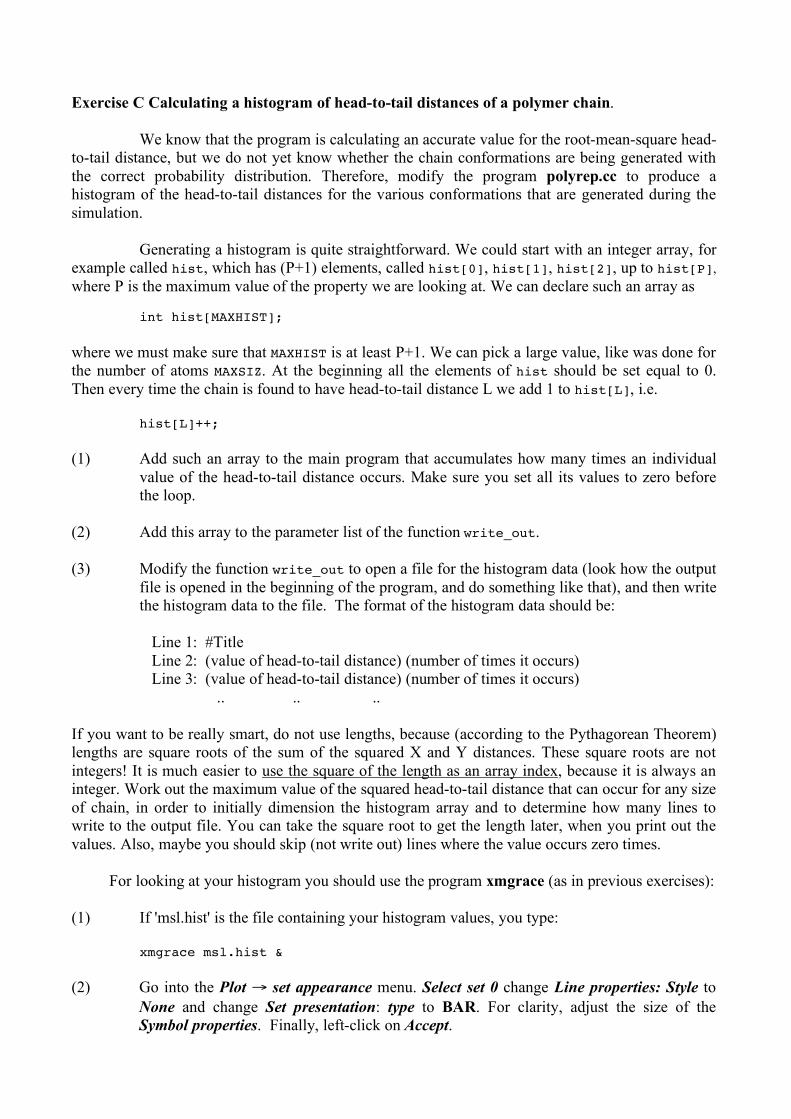
Exercise C Calculating a histogram of head-to-tail distances of a polymer chain. We know that the program is calculating an accurate value for the root-mean-square head-to-tail distance, but we do not yet know whether the chain conformations are being generated with the correct probability distribution. Therefore, modify the program polyrep.cc to produce a histogram of the head-to-tail distances for the various conformations that are generated during the simulation. Generating a histogram is quite straightforward. We could start with an integer array, for example called hist, which has (P+1) elements, called hist[0], hist[1], hist[2], up to hist[P], where P is the maximum value of the property we are looking at. We can declare such an array as int hist[MAXHIST]; where we must make sure that MAXHIST is at least P+1. We can pick a large value, like was done for the number of atoms MAXSIZ. At the beginning all the elements of hist should be set equal to 0. Then every time the chain is found to have head-to-tail distance L we add 1 to hist[L], i.e. hist[L]++; (1) Add such an array to the main program that accumulates how many times an individual

value of the head-to-tail distance occurs. Make sure you set all its values to zero before the loop.

(2) Add this array to the parameter list of the function write_out. (3) Modify the function write_out to open a file for the histogram data (look how the output

file is opened in the beginning of the program, and do something like that), and then write the histogram data to the file. The format of the histogram data should be:

Line 1: #Title Line 2: (value of head-to-tail distance) (number of times it occurs) Line 3: (value of head-to-tail distance) (number of times it occurs)

.. .. .. If you want to be really smart, do not use lengths, because (according to the Pythagorean Theorem) lengths are square roots of the sum of the squared X and Y distances. These square roots are not integers! It is much easier to use the square of the length as an array index, because it is always an integer. Work out the maximum value of the squared head-to-tail distance that can occur for any size of chain, in order to initially dimension the histogram array and to determine how many lines to write to the output file. You can take the square root to get the length later, when you print out the values. Also, maybe you should skip (not write out) lines where the value occurs zero times. For looking at your histogram you should use the program xmgrace (as in previous exercises): (1) If 'msl.hist' is the file containing your histogram values, you type: xmgrace msl.hist & (2) Go into the Plot → set appearance menu. Select set 0 change Line properties: Style to

None and change Set presentation: type to BAR. For clarity, adjust the size of the Symbol properties. Finally, left-click on Accept.

16

(3) Go into Plot → Axis properties menu. For clarity, adjust the range of X axis and Y axis.

In menu Axis label, add suitable labels. (4) Add a title, subtitle by going into the Plot → Graph appearance menu, and picking the

Titles... option. Use your modified program to produce a histogram for the head-to-tail distance of the 5 atom chain described earlier (Natom=5, run for NTimes=200000 steps). How do the results compare to the theoretical predictions? Re-run your program for a chain of length 21 units (Natom=21). NTimes=30000 steps should be sufficient. Produce a histogram and from it estimate how many different head-to-tail distances the 21 atom chain can adopt. What does this tell you about the number of conformations the chain can adopt? For your written report include plots of your two histograms. Also include a printout of the changes you have made to the program.

17

5 References - Flory, P. J. "Statistical mechanics of chain molecules". Wiley, New York, 1969. - Baumgärtner, A. "Simulations of polymer models". In "Applications of the Monte Carlo method in statistical physics", ed. Binder, K. Springer-Verlag, Berlin, 1987. - Lowry, G. G. (ed.) "Markov chains and Monte Carlo calculations in polymer science". Dekker, New York, 1976. - Wall, F. T., Mandel, F. "Macromolecular dimensions obtained by an efficient Monte Carlo method without sample

attrition". J. Chem. Phys., 63 (1975) 4592-5

18

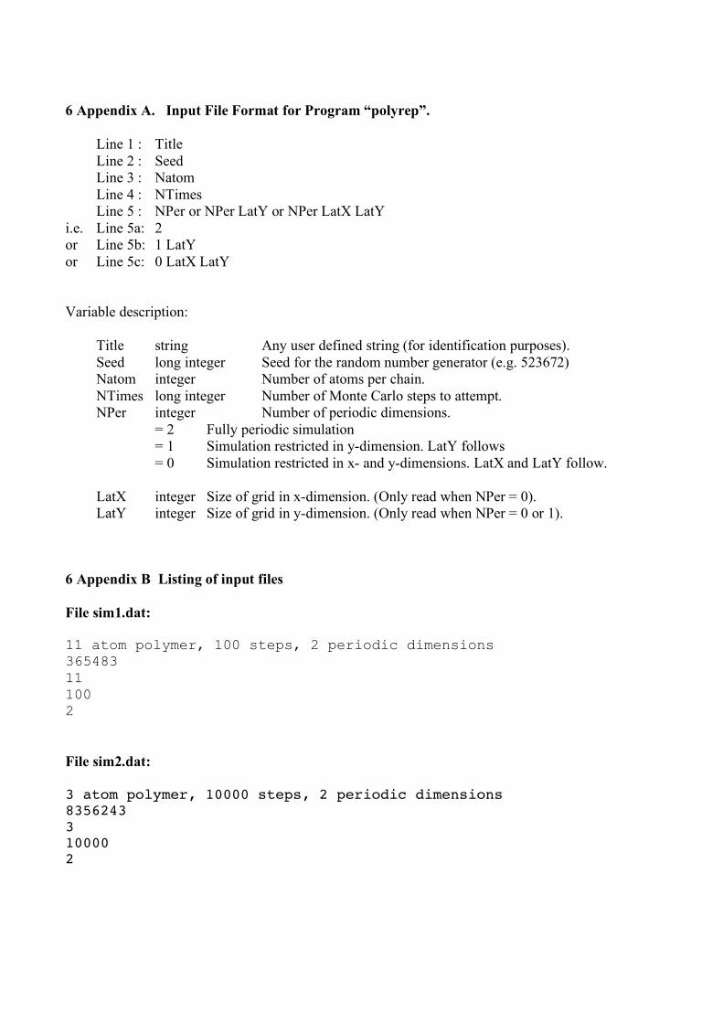
6 Appendix A. Input File Format for Program “polyrep”. Line 1 : Title Line 2 : Seed Line 3 : Natom Line 4 : NTimes Line 5 : NPer or NPer LatY or NPer LatX LatY i.e. Line 5a: 2 or Line 5b: 1 LatY or Line 5c: 0 LatX LatY Variable description: Title string Any user defined string (for identification purposes). Seed long integer Seed for the random number generator (e.g. 523672) Natom integer Number of atoms per chain. NTimes long integer Number of Monte Carlo steps to attempt. NPer integer Number of periodic dimensions. = 2 Fully periodic simulation = 1 Simulation restricted in y-dimension. LatY follows = 0 Simulation restricted in x- and y-dimensions. LatX and LatY follow. LatX integer Size of grid in x-dimension. (Only read when NPer = 0). LatY integer Size of grid in y-dimension. (Only read when NPer = 0 or 1). 6 Appendix B Listing of input files File sim1.dat: 11 atom polymer, 100 steps, 2 periodic dimensions 365483 11 100 2 File sim2.dat: 3 atom polymer, 10000 steps, 2 periodic dimensions 8356243 3 10000 2

19

6 Appendix C Listing of the polyrep program (polyrep.cc) // // PolyRep // // A program for performing simulation of a polymer // on a grid, using a polymer reptation Monte Carlo // algorithm. // // // Original Pascal program by Paul King, 1990 // Modified by Albert Widmann, 1993 // Marcel Zehnder, 1996 // Heiko Sch"afer, 1997 // Translated into C++ by Tomas Hansson, 2000 // #include <iostream> #include <iomanip> #include <string> #include <cmath> #include <fstream> using namespace std; // ============= // Constants // ============= const int MAXSIZ = 300; // Max allowed polymer size // ====================== // Global variables // ====================== long int rseed=12345; // random number generator seed ofstream outfile("polyrep.out"); // output file // =========================== // Function declarations // =========================== double random(long int &random_seed); void pbc(const int latX, // size of grid x dimension const int latY, // size of grid y dimension const int periodicity_flag, // number of periodic dimensions (0,1,2) int &X, // x coordinate to change int &Y); // y coordinate to change void gather(const int natom, // number of atoms in polymer const int lattice_size, // size of dimension to gather const int polymer[], // polymer to gather int gathered[]); // the gathered polymer bool gen_con(const int natom, // number of atoms in polymer const int latX, // lattice size x dimension const int latY, // lattice size y dimension const int periodicity_flag, // int polymerX[], int polymerY[]); // outputs true if generation of initial coordinates succeded void draw_grid(const int natom, // number of atoms in polymer const int latX, // lattice size x dimension const int latY, // lattice size y dimension const int polymerX[], // x coordinates of polymer const int polymerY[]); // y coordinates of polymer bool swap_head(const int natom, // number of atoms in polymer int polymerX[], // x coordinates of polymer int polymerY[]); // y coordinates of polymer // outputs true if a swap of head occured, false otherwise

20

bool make_move(const int natom, // number of atoms in polymer const int latX, // lattice size x dimension const int latY, // lattice size y dimension const int periodicity_flag, // number of periodic dims (0,1,2) int polymerX[], // x coordinates of polymer int polymerY[]); // y coordinates of polymer // outputs true if the move attempt succeded, false otherwise void get_len2(const int natom, // number of atoms in polymer const int latX, // lattice size x dimension const int latY, // lattice size y dimension const int periodicity_flag, // number of periodic dims (0,1,2) const int polymerX[], // x coordinates of polymer const int polymerY[], // y coordinates of polymer long int &Rij2 ); // where the result (square length) comes void write_out(const int natom, // number of atoms in polymer const int latX, // lattice size x dimension const int latY, // lattice size y dimension const int periodicity_flag, // number of periodic dims (0,1,2) const long int ntimes, // number of attempted moves const long int nsucc, // number of successful moves const long int nswap, // number of head swaps const double rate, // rate of success const double RMSL ); // root-mean-square head to tail dist bool read_in(int &natom, // number of atoms in polymer int &latX, // lattice size x dimension int &latY, // lattice size y dimension long int &ntimes, // number of attempted reptation moves int &periodicity_flag, // number of periodic dimensions (0,1,2) int polymerX[], // x coordinates of polymer int polymerY[], // y coordinates of polymer long int &rseed); // random number generator seed // outputs true if reading in went OK, otherwise false // ================== // Main program // ================== int main() { // the variables that describe the polymer configuration int polyX[MAXSIZ],polyY[MAXSIZ]; // polymer coordinates int latsizX=1, latsizY=1; // sizes of lattice where the polymer lives int perflag=0; // number of periodic dimensions of lattice int polylen=1; // number of atoms in polymer long int nummoves=1; // number of reptation moves to attempt // other stuff bool resultflag=false; // read the input file and set up the configuration resultflag= read_in(polylen, latsizX,latsizY, nummoves, perflag, polyX,polyY, rseed); if (!(resultflag)) { cout << endl << endl; cout << "Error when setting up system. Quitting program." << endl; return 1; } // plot initial configuration draw_grid(polylen,latsizX,latsizY,polyX,polyY); double RMSL = 0.0; // keeps RMS long int NSwap = 0; // keeps number of times head swap occured long int NSucc = 0; // keeps number of successful moves // **** MONTE CARLO MAIN LOOP BEGINS HERE **** long int attempt; for (attempt=0; attempt<nummoves; attempt++) {

21

// randomly pick head end of polymer, count swaps resultflag=swap_head(polylen,polyX,polyY); if (resultflag) { NSwap++; } // make a random move of the polymer, count successes resultflag=make_move(polylen,latsizX,latsizY,perflag,polyX,polyY); if (resultflag) { NSucc++; } // keep account of sum of square lengths long int tempsqlen; get_len2(polylen,latsizX,latsizY,perflag,polyX,polyY,tempsqlen); RMSL = RMSL + double(tempsqlen); } // **** MONTE CARLO MAIN LOOP ENDS HERE **** // calculate mean head-to-tail distance, and write to screen // This is where one can get a small overview of the results // of a run, by writing a line of the interesting data from the run. // This can be especially good if one is making many runs and // redirecting screen output to be appended to a file summarizing // all the results. Something missing you would need? Add a cout line! RMSL = sqrt(RMSL / nummoves); double Rate = double(NSucc) / double(nummoves); cout << nummoves << " "; cout << RMSL << " "; cout << Rate << endl; // look at the final configuration draw_grid(polylen,latsizX,latsizY,polyX,polyY); // write results to the output file write_out(polylen,latsizX,latsizY,perflag, nummoves,NSucc,NSwap,Rate,RMSL); // close output file outfile.close(); } /* end of main program */ // ========================== // Function definitions // ========================== double random(long int &random_seed) { // You can treat this function as a "black box" that // gives a random number between 0.0 and 1.0 // The main program must keep a long integer random seed // between calls. // After R Geurtsen, Groningen, 1987 // Calculates seed(new) = ( seed(old)*mult + 1 ) mod m_2 // and random number r = ( seed(new)- (seed(new) mod 10) ) / m_2 // Uses clever integer aritmetics to prevent overflow problems const long int m = 10000L; const long int m_2 = m*m; // max size of seed const long int mult = 31415821L; const long int multh = mult / m; // "high part" of mult const long int multl = mult % m; // "low part" of mult long int irand,irandh,irandl; double r; if (random_seed < 0) { // take absolute value of input seed irand = -(random_seed); } else {

22

irand = random_seed; } irand = irand % m_2; // truncate input seed if too large irandh= irand / m; // "high part" of irand irandl= irand % m; // "low part" of irand // seed * mult can become very large. Therefore now a trick: // high parts are 0 modulo m, so product is 0 modulo m_2 // no need to calculate that part then, therefore no risk of overflow irand =((irandh*multl+irandl*multh) % m)*m + irandl*multl; irand = (irand+1) % m_2; r = (irand / long (10)) * double(10.0); // cut off last digit of irand r = r / double(m_2); // and force between 0 and 1 if ((r < 0.0) || (r >= 1.0)) { // set to 0.0 if something anyway went wrong r=0.0; } random_seed=irand; // store the new random seed for next round return r; } /* End of random */ /*--------------------------------------------------------------------------*/ void pbc(const int latX, // size of grid x dimension const int latY, // size of grid y dimension const int periodicity_flag, // number of periodic dimensions (0,1,2) int &X, // x coordinate to change int &Y) { // y coordinate to change // X and Y before contain atom coordinates // X and Y after contain periodically corrected atom coordinates switch (periodicity_flag) { case 0: // System is finite. No periodic dimensions break; case 1: // System is periodic in x dimension if (X >= latX) { X = X - latX; } else if (X < 0) { X = X + latX; } break; case 2: // System is periodic in x and y dimensions if (X >= latX) { X = X - latX; } else if (X < 0) { X = X + latX; } if (Y >= latY) { Y = Y - latY; } else if (Y < 0) { Y = Y + latY; } break; default: // do nothing if not 0, 1 or 2 break; } } /* End of pbc */ /*--------------------------------------------------------------------------*/ void gather(const int natom, // number of atoms in polymer const int lattice_size, // size of dimension to gather const int polymer[], // polymer to gather int gathered[]) { // the gathered polymer // Due to periodic boundary conditions, polymers are not always // represented as continuous chains in memory. But operations like // reptation moves and center-of-mass calculations are easier to // program if the polymer is first gathered together into a continuous // polymer entity. The periodicity can be restored later. // Takes a periodic set of coordinates for a polymer chain and

23

// gives a continuous, but no longer periodic, set of coordinates. // This is done for one dimension: X or Y. To do both, use twice. for (int i=0; i<natom; i++) { // copy the polymer over gathered[i]=polymer[i]; } for (int i=0; i<natom-1; i++) { // Is there a more than one unit coordinate jump between monomers? // Then that jump must be removed to get a continuous polymer! int dif = polymer[i+1] - polymer[i]; // if jump up, shift rest of chain down one lattice size if (dif > 1) { for (int j=i+1; j < natom; j++) { gathered[j]=gathered[j]-lattice_size; } } // if jump down, shift rest of chain up one lattice size else if (dif < -1) { for (int j=i+1; j < natom; j++) { gathered[j]=gathered[j]+lattice_size; } } } } /* End of gather */ /*--------------------------------------------------------------------------*/ bool gen_con(const int natom, // number of atoms in polymer const int latX, // lattice size x dimension const int latY, // lattice size y dimension const int periodicity_flag, // int polymerX[], int polymerY[]) { // outputs true if generation of initial coordinates succeded // Generates random starting conformation of a natom polymer on // a grid of dimensions latX x latY bool looking=true; const int maxrestarts=15; int restarts=0; const int maxtrials=3000; for (int atom=0; atom< natom; atom++) { int trials=0; looking=true; while ((looking) && (trials < maxtrials) ){ trials++; if (atom > 0) { // choose one of 4 adjacent positions int direction=int(random(rseed)*4); // random 0,1,2 or 3 switch(direction) { case 0: polymerX[atom]=polymerX[atom-1] + 1; polymerY[atom]=polymerY[atom-1]; break; case 1: polymerX[atom]=polymerX[atom-1] - 1; polymerY[atom]=polymerY[atom-1]; break; case 2: polymerX[atom]=polymerX[atom-1]; polymerY[atom]=polymerY[atom-1] + 1; break; case 3: polymerX[atom]=polymerX[atom-1]; polymerY[atom]=polymerY[atom-1] - 1; break; } } else { // start a new chain in a random position atom=0; // correct atom number from restart int pos=int(random(rseed) * latX); polymerX[0] =pos;

24

pos=int(random(rseed) * latY); polymerY[0] =pos; } // now we have a random atom at polymerX[atom], polymerY[atom] // we must now check that it is a good one // check collision with walls looking=false; switch (periodicity_flag) { case 2: // system is unrestricted by walls, x and y periodic break; case 1: // wall in the y direction, x direction periodic if ((polymerY[atom] >= latY) || (polymerY[atom] < 0)) { looking=true; } break; case 0: // walls in both x and y directions if ((polymerY[atom] >= latY) || (polymerY[atom] < 0)) { looking=true; } if ((polymerX[atom] >= latX) || (polymerX[atom] < 0)) { looking=true; } break; default:// should never happen, this is an error looking=true; } // if no collisions with walls, periodize then check self-avoidance if (!looking) { pbc(latX,latY,periodicity_flag,polymerX[atom],polymerY[atom]); for (int i=0; i<=(atom-1); i++) { if ((polymerX[atom]==polymerX[i]) && (polymerY[atom]==polymerY[i])) { looking=true; } } } } // while looking ... if (trials >= maxtrials) { // if we left while loop because we were bored if (restarts > maxrestarts) { // if we did many restarts w new head return false; // this is not working. BAIL OUT! } else { // let us do a restart from head atom atom=-999; // will be corrected to 0 inside the loop before use looking=true; trials=0; restarts++; } } } // for (int atom= ... return (!looking); } /* End of gen_con*/ /*--------------------------------------------------------------------------*/ void draw_grid(const int natom, // number of atoms in polymer const int latX, // lattice size x dimension const int latY, // lattice size y dimension const int polymerX[], // x coordinates of polymer const int polymerY[]) { // y coordinates of polymer char grid[MAXSIZ][MAXSIZ]; // the grid to print out // initialize grid with dots to mark all spots empty for (int j=0; j< latY; j++) { for (int i=0; i<latX; i++) { grid[i][j]='.'; } }

25

// draw the polymer in the grid: head, body, tail grid[polymerX[0]][polymerY[0]] = 'H'; for (int i=1; i<= natom-2; i++){ grid[polymerX[i]][polymerY[i]] = '0'; } grid[polymerX[natom-1]][polymerY[natom-1]] ='T'; outfile << endl << endl; for (int j=0; j < latY; j++) { for (int i=0; i< latX; i++) { outfile << grid[i][j]; } outfile << endl; } outfile << endl; } /* End of draw_grid */ /*--------------------------------------------------------------------------*/ bool swap_head(const int natom, // number of atoms in polymer int polymerX[], // x coordinates of polymer int polymerY[]) { // y coordinates of polymer // randomly chooses which end of the polymer is head in next move // returns true if a swap of head occured, false otherwise // 50 % chance of swapping gives equal chance for each end to be head // of polymer during the reptation int temp; // place to keep value while swapping int swapupto; // midpoint of the polymer bool do_swap=false; if (random(rseed) > 0.5) { do_swap=true; } if (do_swap) { if ((natom % 2) == 0) { // even number of atoms, find half swapupto=natom / 2; } else { // odd number of atoms: middle one stays unswapped swapupto=(natom-1) / 2; } // swap X coordinates first<-->last, second<-->secondlast etc. for (int i=0; i< swapupto; i++) { temp=polymerX[i]; polymerX[i]=polymerX[(natom-1)-i]; polymerX[(natom-1)-i]=temp; } // swap Y coordinates first<-->last, second<-->secondlast etc. for (int i=0; i< swapupto; i++) { temp=polymerY[i]; polymerY[i]=polymerY[(natom-1)-i]; polymerY[(natom-1)-i]=temp; } } return do_swap; } /* End of swap_head */ /*--------------------------------------------------------------------------*/ bool make_move(const int natom, // number of atoms in polymer const int latX, // lattice size x dimension const int latY, // lattice size y dimension const int periodicity_flag, // number of periodic dims (0,1,2) int polymerX[], // x coordinates of polymer int polymerY[]) { // y coordinates of polymer // outputs true if the move attempt succeded, false otherwise // procedure for attempting to move the polymer: head can move

26

// in any of three forward directions // directions are 0-right 1-left 2-down 3-up int tempX[MAXSIZ]; int tempY[MAXSIZ]; // gather the chain, put in a temporary place gather(natom,latX,polymerX,tempX); gather(natom,latY,polymerY,tempY); // find where second atom is, and do not move there int difX =tempX[1] - tempX[0]; int difY =tempY[1] - tempY[0]; int no_go; if (difX == 1) { no_go = 0; } else if (difX == -1) { no_go = 1; } else if (difY == 1) { no_go = 2; } else if (difY == -1) { no_go = 3; } else { cout << "ERROR" << endl; } // generate a random number not in the backward direction int dir; do { dir = int(random(rseed)*4.0); } while ( (dir == no_go) || (dir < 0) || (dir > 3) ); // generate position of new head int newHX, newHY; switch (dir) { case 0: // right newHX = tempX[0] + 1; newHY = tempY[0]; break; case 1: // left newHX = tempX[0] - 1; newHY = tempY[0]; break; case 2: // down newHX = tempX[0]; newHY = tempY[0] + 1; break; case 3: // up newHX = tempX[0] ; newHY = tempY[0] - 1; } // test to see if new head position means hitting the wall bool hit_wall=false; switch (periodicity_flag) { case 0: // periodic in no dimensions means check both walls if ((newHX >= latX) || (newHX < 0) ) { hit_wall = true; } if ((newHY >= latY) || (newHY < 0) ) { hit_wall = true; } break; case 1: // periodic in x, check for wall hit in y direction if ((newHY >= latY) || (newHY < 0) ) { hit_wall = true; } break; case 2: // periodic in two dimension means no walls // nothing to do break; }

27

if (!(hit_wall)) { // apply periodic boundary conditions pbc(latX,latY,periodicity_flag,newHX,newHY); // test that the new head does not collide with the current // polymer configuration except the tail (which will have moved) for (int i=1; i<=natom-2; i++) { if ((newHX==polymerX[i]) && (newHY==polymerY[i])) { hit_wall=true; } } } // if ok so far, reptate the polymer if (!(hit_wall)) { for (int i=natom-1; i>0; i--) { polymerX[i]=polymerX[i-1]; polymerY[i]=polymerY[i-1]; } polymerX[0]=newHX; polymerY[0]=newHY; } // and return status return (!hit_wall); } /* End of make_move */ /*--------------------------------------------------------------------------*/ void get_len2(const int natom, // number of atoms in polymer const int latX, // lattice size x dimension const int latY, // lattice size y dimension const int periodicity_flag, // number of periodic dims (0,1,2) const int polymerX[], // x coordinates of polymer const int polymerY[], // y coordinates of polymer long int &Rij2 ) { // where the result (square length) comes // Takes the current configuration and calculates the square of // the distance between the endpoints of the polymer. // Result comes out in last argument. int tempX[MAXSIZ]; // temporary storage for gathered polymer x coords int tempY[MAXSIZ]; // temporary storage for gathered polymer y coords switch (periodicity_flag) { case 0: // non-periodic system - no gathering needed for (int i=0; i< natom; i++) { tempX[i]=polymerX[i]; tempY[i]=polymerY[i]; } break; case 1: // system is periodic in x direction, so gather that gather(natom,latX,polymerX,tempX); for (int i=0; i< natom; i++) { tempY[i]=polymerY[i]; } break; case 2: // system is periodic in x and y directions, so gather both gather(natom,latX,polymerX,tempX); gather(natom,latY,polymerY,tempY); break; } // now we have the continuous polymer in tempX and tempY // time to calculate what we want to know long int distX,distY,distX2,distY2; distX=tempX[natom-1] - tempX[0]; // Last atom minus first atom x distY=tempY[natom-1] - tempY[0]; // Last atom minus first atom y distX2=distX * distX; // square distY2=distY * distY; Rij2 = distX2 + distY2; // and send off result to caller

28

} /* End of get_len2 */ /*--------------------------------------------------------------------------*/ void write_out(const int natom, // number of atoms in polymer const int latX, // lattice size x dimension const int latY, // lattice size y dimension const int periodicity_flag, // number of periodic dims (0,1,2) const long int ntimes, // number of attempted moves const long int nsucc, // number of successful moves const long int nswap, // number of head swaps const double rate, // rate of success const double RMSL ) { // root-mean-square head to tail dist outfile << " Number of atoms : " << setw(11) << natom << endl; outfile << " Number of periodic dimensions : " << setw(11) << periodicity_flag << endl; outfile << " Lattice size [X,Y] : " << setw(6) << latX << setw(5) << latY << endl; outfile << " Number of attempted moves : " << setw(11) << ntimes << endl; outfile << " Number of successful moves : " << setw(11) << nsucc << endl; outfile << " Acceptance ratio : " << setw(11) << setprecision(4) << rate << endl; outfile << " Number of head/tail swaps : " << setw(11) << nswap << endl; outfile << "Root-mean-square head to tail distance : " << setw(11) << setprecision(4) << RMSL << endl; outfile << " Atom density : " << setw(11) << setprecision(4) << double(natom) / double(latX*latY) << endl; outfile << endl; } /* End of write_out */ /*--------------------------------------------------------------------------*/ bool read_in(int &natom, // number of atoms in polymer int &latX, // lattice size x dimension int &latY, // lattice size y dimension long int &ntimes, // number of attempted reptation moves int &periodicity_flag, // number of periodic dimensions (0,1,2) int polymerX[], // x coordinates of polymer int polymerY[], // y coordinates of polymer long int &rseed) { // random number generator seed // returns true if reading in went OK, otherwise false // reads in control options to the program and sets up the // system according to these control options // The input is read from standard input, and an input file should // have the following format: // Line 1: Title (a text string describing the run) // Line 2: Random number seed (an integer > 0) // Line 3: Number of atoms in the polymer (minimum 2) // Line 4: Number of reptation moves (>=1) // Line 5: Number of periodic dimensions and sizes of nonperiodic dimensions // i.e. 5a: 0 xsize ysize // or 5b: 1 ysize // or 5c: 2 // Read line 1: title string title_string; getline(cin,title_string); // read full line of text, do not stop at space outfile << endl << "Title from data file :" << endl << title_string << endl << endl; // Read line 2: random seed cin >> rseed; outfile << "SEED= " << rseed << endl; // Read line 3: number of atoms

29

cin >> natom; if ((natom < 2) || (natom > MAXSIZ)) { cout << "Illegal number of atoms: " << natom << endl; return false; } latX = natom; // default x size of grid before we know size/periodicity latY = natom; // default y size of grid before we know size/periodicity // Read line 4: number of moves cin >> ntimes; if (ntimes < 1) { cout << "Illegal number of moves: " << ntimes << endl; return false; } // Read line 5: periodicity and sizes of non-periodic dimensions cin >> periodicity_flag; if (! ((periodicity_flag==0) || (periodicity_flag==1) || (periodicity_flag==2)) ) { cout << "Illegal number of periodic dimensions: "; cout <<periodicity_flag << endl; return false; } switch (periodicity_flag) { case 0: // both x and y dimensions are non-periodic, so read their sizes cin >> latX; cin >> latY; break; case 1: // x dimension is non-periodic, so read its size cin >> latY; break; case 2: //nothing to do break; default: return false; } if ((latX < 1) || (latX > MAXSIZ)) { cout << "Illegal size of lattice x dimension: " << latX << endl; return false; } if ((latY < 1) || (latY > MAXSIZ)) { cout << "Illegal size of lattice y dimension: " << latY << endl; return false; } bool went_ok=true; // make random starting configuration went_ok=gen_con(natom,latX,latY,periodicity_flag,polymerX,polymerY); return went_ok; } /* End of read_in */ /*--------------------------------------------------------------------------*/