Cyclic Homology Theory

Jean-Louis Loday

Notes taken by

Pawe l Witkowski

October 2006

Contents

1 Cyclic category 3

1.1 Circle and disk as a cell complexes . . . . . . . . . . . . . . . . . . . . . . . . 31.2 Simplicial sets . . . . . . . . . . . . . . . . . . . . . . . . . . . . . . . . . . . . 71.3 Fibrations . . . . . . . . . . . . . . . . . . . . . . . . . . . . . . . . . . . . . . 101.4 Cyclic category . . . . . . . . . . . . . . . . . . . . . . . . . . . . . . . . . . . 111.5 Noncommutative sets . . . . . . . . . . . . . . . . . . . . . . . . . . . . . . . . 131.6 Adjoint functors . . . . . . . . . . . . . . . . . . . . . . . . . . . . . . . . . . 141.7 Generic example of a simplicial set . . . . . . . . . . . . . . . . . . . . . . . . 151.8 Simplicial modules . . . . . . . . . . . . . . . . . . . . . . . . . . . . . . . . . 201.9 Bicomplexes . . . . . . . . . . . . . . . . . . . . . . . . . . . . . . . . . . . . . 211.10 Spectral sequences . . . . . . . . . . . . . . . . . . . . . . . . . . . . . . . . . 23

2 Cyclic homology 27

2.1 The cyclic bicomplex . . . . . . . . . . . . . . . . . . . . . . . . . . . . . . . . 272.2 Characteristic 0 case . . . . . . . . . . . . . . . . . . . . . . . . . . . . . . . . 292.3 Computations . . . . . . . . . . . . . . . . . . . . . . . . . . . . . . . . . . . . 302.4 Periodic and negative cyclic homology . . . . . . . . . . . . . . . . . . . . . . 332.5 Harrison homology . . . . . . . . . . . . . . . . . . . . . . . . . . . . . . . . . 342.6 Derived functors . . . . . . . . . . . . . . . . . . . . . . . . . . . . . . . . . . 35

3 Relation with K-theory 37

3.1 K-theory . . . . . . . . . . . . . . . . . . . . . . . . . . . . . . . . . . . . . . . 373.2 Trace map . . . . . . . . . . . . . . . . . . . . . . . . . . . . . . . . . . . . . . 383.3 Algebraic K-theory . . . . . . . . . . . . . . . . . . . . . . . . . . . . . . . . . 40

2

Chapter 1

Cyclic category

1.1 Circle and disk as a cell complexes

The circle in its simplest decomposition has one 0-cell (a point) and one 1-cell (an interval).

Figure 1.1: Circle

This is the only way to form a circle from an interval. If we try to decompose a diskof higher dimension, then we have choices. In the table below we give a few examples ofdecomposition of an n-cell.

3

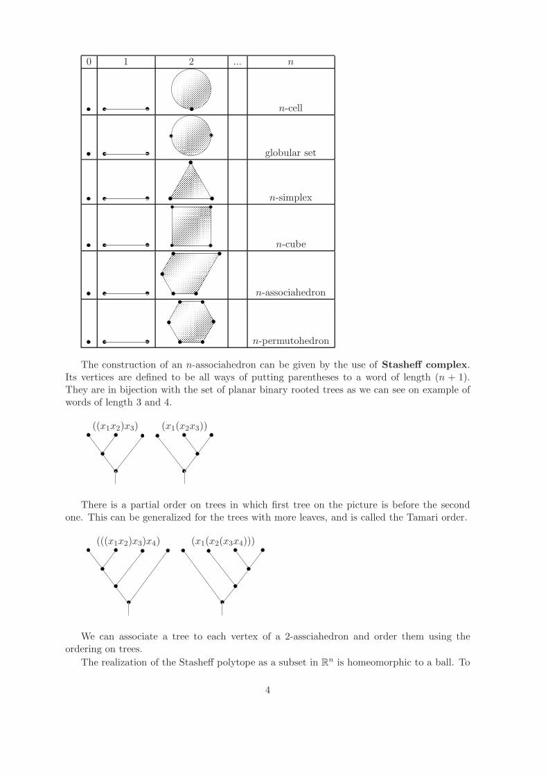
0 1 2 ... n

n-cell

globular set

n-simplex

n-cube

n-associahedron

n-permutohedron

The construction of an n-associahedron can be given by the use of Stasheff complex.Its vertices are defined to be all ways of putting parentheses to a word of length (n + 1).They are in bijection with the set of planar binary rooted trees as we can see on example ofwords of length 3 and 4.

((x1x2)x3) (x1(x2x3))

There is a partial order on trees in which first tree on the picture is before the secondone. This can be generalized for the trees with more leaves, and is called the Tamari order.

(((x1x2)x3)x4) (x1(x2(x3x4)))

We can associate a tree to each vertex of a 2-assciahedron and order them using theordering on trees.

The realization of the Stasheff polytope as a subset in Rn is homeomorphic to a ball. To

4

each planar binary tree t we associate a point M(t) = (x1, . . . , xn) in Rn as follows. The i-thcoordinate is the product of the number of leaves to the left of i-th vertex times the numberof leaves to the right.

1

2

3

4

Figure 1.2: Tree t

M(t) = (1 · 1, 2 · 1, 3 · 2, 1 · 1) = (1, 2, 6, 1) ∈ R4

The Stasheff polytope of dimension n is the convex hull of the points M(t) for all planarbinary trees with (n+ 1) leaves. The sum of coordinates is

n∑

i=1

xi =n(n+ 1)

2

so the Stasheff polytope lies in the hyperplane given by this equation. The examples ofStasheff polytopes K1 and K2 are in the following pictures.

21

1

2 (1,2)

(2,1)

The Stasheff polytope K3 has 14 vertices and 7 faces. The faces are three squares andfour pentagons (2-associahedrons). In general, the Stasheff polytope Kn has faces of the formKp ×Kq, where p+ q = n.

What about the permutohedron? Take an element σ in the symmetric group Sn. Associateto it the pointM(σ) = (σ(1), . . . , σ(n)) ∈ Rn. Then we have permutohedron Pn−1 as a convex

hull of all points M(σ) for all permutations. Of course∑n

i=1 σ(i) = n(n+1)2 , so it lies in the

hyperplane given by the equation∑n

i=1 xi = n(n+1)2 .

In general Pn has faces of the form Pp × Pq, where p+ q = n− 1.

Observe that we have an order on vertices of our complexes.

5

Figure 1.3: 2-permutohedron

On the set of vertices of n-simplex the order comes from the order on natural numbers,because vertices are numbered from 0 to n.

On the set of vertices n-associahedron the order is called the Tamari order.

Figure 1.4: Tamari order on trees

On n-permutohedrons the order comes from the weak Bruhat order on the symmetricgroup Sn.

6

1.2 Simplicial sets

Definition 1.1. The n-simplex is a ssubspace ∆n = (x0, . . . , xn) ∈ Rn+1 :∑

i xi = 1, 0 ≤xi ≤ 1. Denote by i the vertex on the xi-axis.

On the set of vertices of an n-simplex we have an ordering coming from the order on theset [n] = 0, . . . , n.

1

0

0

1

2

0

1

2

3

Definition 1.2. Define two kinds of order preserving maps on simplexes

• Face maps δi : ∆n−1 → ∆n, i = 0, . . . , n, whose image is the face not containing i asimage,

δi(x0, . . . , xn−1) = (x0, . . . , xi−1, 0, xi+1, . . . , xn)

• Degeneracy maps σj : ∆n+1 → ∆n, j = 0, . . . , n which squeeze the j-th face.

σj(x0, . . . , xn+1) = (x0, . . . , xj−1, xj + xj+1, xj+2, . . . , xn+1)

Degeneracy map which does not preserve the ordering on vertices is not allowed. Forexample if n = 2 we have two allowed degeneracies s0, s1

The face and degeneracy maps satisfy the following identities

δjδi = δiδj−1, i < j

σjσi = σiσj+1, i ≤ j

σjδi =

δiσj−1 i < j

id i = j, i = j + 1

δi−1σj i > j + 1

Definition 1.3. A simplicial set is a collection of sets Knn≥0 with a collection of maps

di : Kn → Kn−1, i = 0, . . . , n

sj : Kn → Kn+1, j = 0, . . . , n

7

satisfying ”the dual relations”

didj = dj−1di, i < j

sisj = sj+1si, i ≤ j

djsi =

sj−1di i < j

id i = j, i = j + 1

sjdi−1 i > j + 1

A simplicial morphism ϕ• : K• → K ′• is a collection of maps ϕn : Kn → K ′

n which commutewith face and degeneracy maps

Knϕn //

dKi K ′

n

dK′

iKn−1 ϕn−1

// K ′n−1

Kn+1ϕn+1 // K ′

n+1

Kn ϕn

//sKj

OOK ′n

sK′

j

OONow suppose we have a simplicial set K•. For all x ∈ Kn we take a simplex ∆n and we

will build a topological space out of these data.

The geometric realization of a simplicial set is the following topological space

∣∣X•

∣∣ :=∐

n≥0

Xn ×∆n/ ∼,

where the equivalence relation ∼ is defined as follows. We identify (x, δit) ∈ Xn × ∆n

with (dix, t) ∈ Xn−1 × ∆n−1 for any x ∈ Xn, t ∈ ∆n−1 and (x, σjt) ∈ Xn × ∆n with(sjx, t) ∈ Xn+1×∆n+1 for any x ∈ Xn−1 and t ∈ ∆n+1. The topology on |X•| is the quotienttopology.

There exists a simplicial category ∆, whose objects are finite ordered sets [n] =0, . . . , n, and morphism Mor([n], [m]) are nondecreasing set maps.

The category ∆ can be described by generators and relations. As generators we take faceand degeneracy maps

δi : [n− 1]→ [n]

σj : [n+ 1]→ [n]

and relations are as before

δjδi = δiδj−1, i < j

σjσi = σiσj+1, i ≤ j

σjδi =

δiσj−1 i < j

id i = j, i = j + 1

δi−1σj i > j + 1

Example 1.4. Take Xn = ∗ for all n ≥ 0, di, sj- the identity. Then |∗| = ∗.

8

Example 1.5. Take a monoid M (or a group). Define M• as follows.

Mn := M × . . .×︸ ︷︷ ︸n times

M = Mn

di(m1, . . . ,mn) =

(m2, . . . ,mn) i = 0

(m1, . . . ,mimi+1, . . . ,mn) 0 < i < n

(m1, . . . ,mn−1) i = n

sj(m1, . . . ,mn) = (m1, . . . ,mj , 1,mj+1, . . . ,mn)

Example 1.6. Let C be a small category. The nerve of C is the following simplicial set

Cn := C0f1−→ C1

f2−→ . . .

fn−→ Cn

di(C0f1−→ C1

f2−→ . . .

fn−→ Cn) = forget about Ci

= (C0f1−→ C1

f2−→ . . .→

→ Ci−1fi+1fi−−−−→ Ci+1 → . . .

fn−→ Cn)

sj(C0f1−→ C1

f2−→ . . .

fn−→ Cn) = insert idCj

= (C0f1−→ C1

f2−→ . . .→

→ Cj−1fj−→ Cj

id−→ Cj

fj+1−−−→ Cj+1 → . . .

fn−→ Cn)

The axioms of a category are exactly the conditions for C• to be a simplicial set.

f g f g

h

hg

gfgf

h(gf)=(hg)f

Figure 1.5: Associativity relation

To each category we associate its classifying space

B C := |C•|

The classifying space BG of a group G is obtained from the realization of simplicial set inexample (1.5). If G is discrete, then we can prove the following

π1(BG) = G

πn(BG) = 0, n ≥ 1.

If all Xn are topological spaces, and the face and degeneracy maps are continuous, thenwe call X• a simplicial space. Then the geometric realization is defined as before, but wekeep track of the topology of Xn in the construction.

∣∣X•

∣∣ :=∐

n≥0

Xn ×∆n/ ∼,

9

(x, δit) ∼ (dix, t)

(x, σjt) ∼ (sjx, t)

1.3 Fibrations

A locally trivial fibration is a surjective map of topological spaces f : E → B such thatfor every b ∈ B there exists a neighbourhood Ub of b in B such that f−1(Ub) ≃ Ub×F , whereF is a fiber.

Example 1.7. The Mobius band is a fibration over S1. It is not a trivial fibration because itis not a product.

There is a fibration

G→ EG→ BG

where EG is a contractible space. For example if G = Z, then this fibration is homotopyequivalent to

Z→ R→ S1

But B Z is not a space with one 0-cell and one 1-cell. The 0-cells are in bijection with Z,

Figure 1.6: Z → R→ S1

and 1-cells are in bijection with pairs of distinct integers.

Example 1.8. The Hopf fibration it is a map f : S3 → S2 with fiber S1 which can bedescribed as follows.

S3 := (z, z′) : |z|2 + |z′|2 = 1 ⊂ C× C

S2 := (t, z) : t2 + |z|2 = 1 ⊂ R× C

f(z, z′) = (|z|2 − |z′|2, 2zz′) ∈ R× C

The restriction of f to the north (resp. south) hemisphere is a trivial fibration.

Another description of the sphere S3 is given by gluing two solid tori S1×D2 and D2×S1

along the boundary S1 × S1.

If X and Y are pointed spaces, then we can perform the join construction X ∗ Y .

X ∗ Y := X × I × Y/ ∼,

10

8

Figure 1.7: S3 = S1 ×D2 ∪S1×S1 D2 × S1

(x, 0, ∗) ∼ (x′, 0, ∗)

(∗, 1, y) ∼ (∗, 1, y)

For example S1 ∗ S1 = S3.

Exercise 1.9. Show that ∆p ∗∆q ≃ ∆p+q+1.

1.4 Cyclic category

We know, that B Z is homotopy equivalent to S1. Consider a question: what is the simplicialset C• whose geometric realization is the circle with the cell structure consisting of one 0-celland one 1-cell (not up to homotopy)?

The 0-cell ∗ ∈ C0 generates only one element, still denoted by ∗ in each Cn. Suppose weadd an additional element τ to C1. Then we get

C0 = ∗

C1 = ∗, τ

C2 = ∗, s0τ, s1τ

C3 = ∗, s1s0τ, s2s0τ, s2s1τ

. . . . . .

Cn = ∗, . . . , sn−1 . . . si, . . . s0τ, . . .

The faces are obvious to find. In particular d0(τ) = ∗ = d1(τ). Then the geometric realization|C•| is a circle with its simplest cell structure. We can identify

Cn = ∗, . . . , sn−1 . . . si, . . . s0τ, . . .

11

with the cyclic group Z/(n + 1)Z =: Cn by sending ∗ to 0, and sn−1 . . . si, . . . s0τ to i + 1.Denote the generator of Cn by tn.

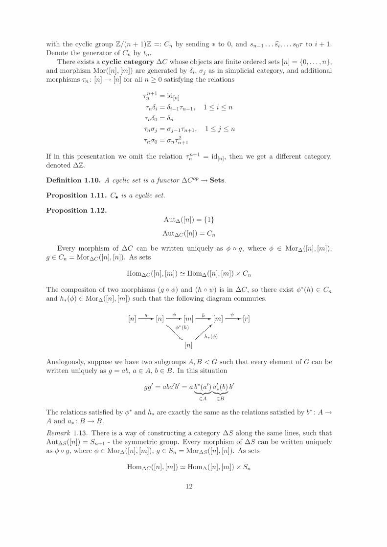
There exists a cyclic category ∆C whose objects are finite ordered sets [n] = 0, . . . , n,and morphism Mor([n], [m]) are generated by δi, σj as in simplicial category, and additionalmorphisms τn : [n]→ [n] for all n ≥ 0 satisfying the relations

τn+1n = id[n]

τnδi = δi−1τn−1, 1 ≤ i ≤ n

τnδ0 = δn

τnσj = σj−1τn+1, 1 ≤ j ≤ n

τnσ0 = σnτ2n+1

If in this presentation we omit the relation τn+1n = id[n], then we get a different category,

denoted ∆Z.

Definition 1.10. A cyclic set is a functor ∆Cop → Sets.

Proposition 1.11. C• is a cyclic set.

Proposition 1.12.

Aut∆([n]) = 1

Aut∆C([n]) = Cn

Every morphism of ∆C can be written uniquely as φ g, where φ ∈ Mor∆([n], [m]),g ∈ Cn = Mor∆C([n], [n]). As sets

Hom∆C([n], [m]) ≃ Hom∆([n], [m]) × Cn

The compositon of two morphisms (g φ) and (h ψ) is in ∆C, so there exist φ∗(h) ∈ Cnand h∗(φ) ∈ Mor∆([n], [m]) such that the following diagram commutes.

[n]g // [n]

φ //φ∗(h) AAAAAAAA [m]

h // [m]ψ // [r]

[n]

h∗(φ)

==||||||||Analogously, suppose we have two subgroups A,B < G such that every element of G can bewritten uniquely as g = ab, a ∈ A, b ∈ B. In this situation

gg′ = aba′b′ = a b∗(a′)︸ ︷︷ ︸∈A

a′∗(b)︸ ︷︷ ︸∈B

b′

The relations satisfied by φ∗ and h∗ are exactly the same as the relations satisfied by b∗ : A→A and a∗ : B → B.

Remark 1.13. There is a way of constructing a category ∆S along the same lines, such thatAut∆S([n]) = Sn+1 - the symmetric group. Every morphism of ∆S can be written uniquelyas φ g, where φ ∈ Mor∆([n], [m]), g ∈ Sn = Mor∆S([n], [n]). As sets

Hom∆C([n], [m]) ≃ Hom∆([n], [m]) × Sn

12

It means that for any φ ∈ Mor∆([m], [n]) and σ ∈ Sn there exist φ∗(σ) ∈ Sm+1 and σ∗(φ) ∈Mor∆([m], [n]) such that the following diagram commutes.

[m]φ //

φ∗(g)∈Sn+1 [n]

σ∈Sn+1[n]

σ∗(φ)// [n]

Denote by ∆B the braided category, defined along the same lines using braid groups, which

0

12

3

32

1

00

12

34

03

42

1

Figure 1.8: Morphisms in ∆S

contains ∆S as a quotient category. Let Hn = (Z/2)n ⋊ Sn = Z/2∫Sn and denote corre-

sponding hyperdihedral category by ∆H. Furthermore we have a dihedral category ∆D. Wecan arrange them in a diagram of inclusions

∆C // ∆S // ∆B

∆Z/2 // ∆D // ∆HThere is an exact sequence of groups

0→ Z·(n+1)−−−−→ Z→ Z/(n+ 1)→ 0

If we treat Z as category, then we have following diagram of functors

∆× Z→ ∆Z→ ∆C

We can ask what kind of structure on the geometric realization of the underlying simplicialset X•, that is |X•|, does the cyclic structure give? The answer is a structure of S1-space.An open question is: can we discretize analogously S3 = SU(2)?

1.5 Noncommutative sets

Let Fin denote the skeleton category of the category of finite sets. This means that theobjects in Fin are the sets [n] = 0, 1 . . . , n and morphisms are arbitrary functions. LetFin′ denote a category with the same objects, but whose morphisms satisfy f(0) = 0. Thenthere is a following diagram of categories

∆op // ∆S′op // Fin′∆C = ∆Cop // ∆S // Fin

13

For a set [n] we have

Aut∆S([n]) = Sn+1,

Aut∆S′([n]) = Sn.

The top row of this diagram will correspond to Hochschild homology, and the bottom row tocyclic homology, which we will define in the next chapter.

If A is an algebra, then [n] 7→ A⊗(n+1) is a well defined functor ∆S →Mod.

A⊗2 A, a⊗ b 7→ ab, a⊗ b 7→ ba.

The two maps d1, d0 : [1] → [0] become the same in Fin. If A is commutative, then [n] →A⊗(n+1) factors through Fin.

Thus ∆S can be viewed as a category of noncommutative sets. It has a following descrip-tion

Ob(∆S) = [n]

Mor∆S([n], [m]) = set of maps with an order on the fibers f−1(i) for i ∈ [m].

1.6 Adjoint functors

Suppose we have two categories A and B and a pair of functors F : A → B, G : B → A. Wesay that F is right adjoint to G and G is left adjoint to F if there is an isomorphism ofsets

HomA(G(B), A) ≃ HomB(B,F (A))

for every A ∈ Ob(A), B ∈ Ob(B), and the isomorphism is functorial in A and B.

Example 1.14. Let A,B = Sets. Take a set X and define

G(B) = B ×X, F (A) = HomSets(X,A)

ThenHom(B ×X,A) ≃ Hom(B,Hom(X,A))

ϕ : B ×X → A 7→ (B → Hom(X,A))

Many examples follow the pattern in (1.14), but with additional structure.

Example 1.15. Let A,B = Vect, V vector space over a field k. Define

G(B) = B ⊗k V, F (A) = Homk(V,A)

ThenHomk(B ⊗k V,A) = Homk(B,Homk(V,A))

Example 1.16. Let R be a ring, A be the category of left R-modules, and B the category orright R-modules. Take a left R-module V and define

G(B) = B ⊗R V, F (A) = HomR(V,A)

HomZ(B ⊗R V,A) = HomZ(B,HomR(V,A))

Example 1.17. Define the loop space and the suspension of a topological space X with basepoint as follows.

ΩX = f : S1 → X : f(∗) = ∗

SX = S1 ∧X/S1 ∨X

ThenHomTop∗

(SX, Y ) ≃ HomTop∗(X,ΩY )

where Top∗ is the category of topological spaces with base point.

14

1.7 Generic example of a simplicial set

Let X be a topological space. Define

Sn(X) := f : ∆→ X, continuous

We claim that S•(X) is a simplicial set with the following face and degeneracy maps:

di : Sn(X)→ Sn−1(X), di(f) := f δi

sj : Sn(X)→ Sn+1(X), sj(f) := f σj

It is called the singular functor. It goes from the category of topological spaces to thecategory of simplicial sets.

S•(−) : Top→ SSets

Recall the functor of geometric realization of a simplicial set,

K• 7→ |K•|, | − | : SSets→ Top

Proposition 1.18. The functors S•(−) and | − | are adjoint, that is

HomTop(|K•|,X) ≃ HomSSets(K•,S•(X)).

In the example (1.16) R-modules can be replaced by functors. Left modules correspondto covariant functors, and right modules correspond to contravariant functors. Then thegeometric realization functor can be seen as a tensor product over the simplicial category

|K•| = K• ⊗∆ ∆•

In an analogous way we can present the singular functor as

S•(X) = HomTop(∆•,X)

Hence we can derive adjointness

HomTop(K• ⊗∆ ∆•,X) ≃ Hom∆(K•,HomTop(∆•,X))

Now the question arises: how to compareX and |S•(X)|? Take id ∈ HomSSets(S•(X),S•(X)).This identity goes to a map

ε : |S•(X)| → X

which is called a unit. Also id ∈ HomTop(|K•|, |K•|) goes to a map

η : K• → S•(|K•|)

which is called a counit. If X is a CW-complex, then this map is a homotopy equivalence.Now we will prove the following theorem.

Theorem 1.19. If X• is a cyclic set, then the geometric realization |X•| is an S1-space.

Before the proof, we will give some necessary propositions.

Lemma 1.20. The functor ∆→ Top given by [n] 7→ ∆n is in fact a functor on ∆C (it is acocyclic space).

15

Proof. It is enough to define the image of τn

τn 7→ ∆n → ∆n

vertex i 7→ vertex i− 1

vertex 0 7→ vertex n

Let C• be the cyclic set, whose geometric realization is the circle. A naive way to definean S1-action would be to use

C• ×X• → X•

(g, x) 7→ g∗(x)

But it does not work, since it gives a trivial action of S1 for X• = C•.

There is a forgetful functor from the category of cyclic sets to the category of simplicialsets.

G : CSets→ SSets

We will define its left adjoint

F : SSets→ CSets

If Y• is a simplicial set, then put

F (Y•)n := Cn × Yn, Cn = Z/(n + 1)Z

If f is a morphism in ∆op, then we define

f∗(g, y) := (f∗(g), (g∗(f))∗(y))

[n]f //

f∗(g) [m]

g[n]

g∗(f)// [m]

If h is a morphism in Cm, then we define

h∗(g, y) := (h(g), y)

Proposition 1.21. The set F (Y•) equipped with the simplicial structure given by f∗ and thecyclic structure given by h∗ is a cyclic set.

Proposition 1.22. If X•, Y• are simplicial sets, and if |X•| × |Y•| is a CW-complex, thenthe map

|X• × Y•| → |X•| × |Y•|

is a homeomorphism.

Proposition 1.23. If X• is a cyclic set, then we have a homeomorphism

|F (X•)| ≃ |C•| × |X•| = S1 × |X•|

16

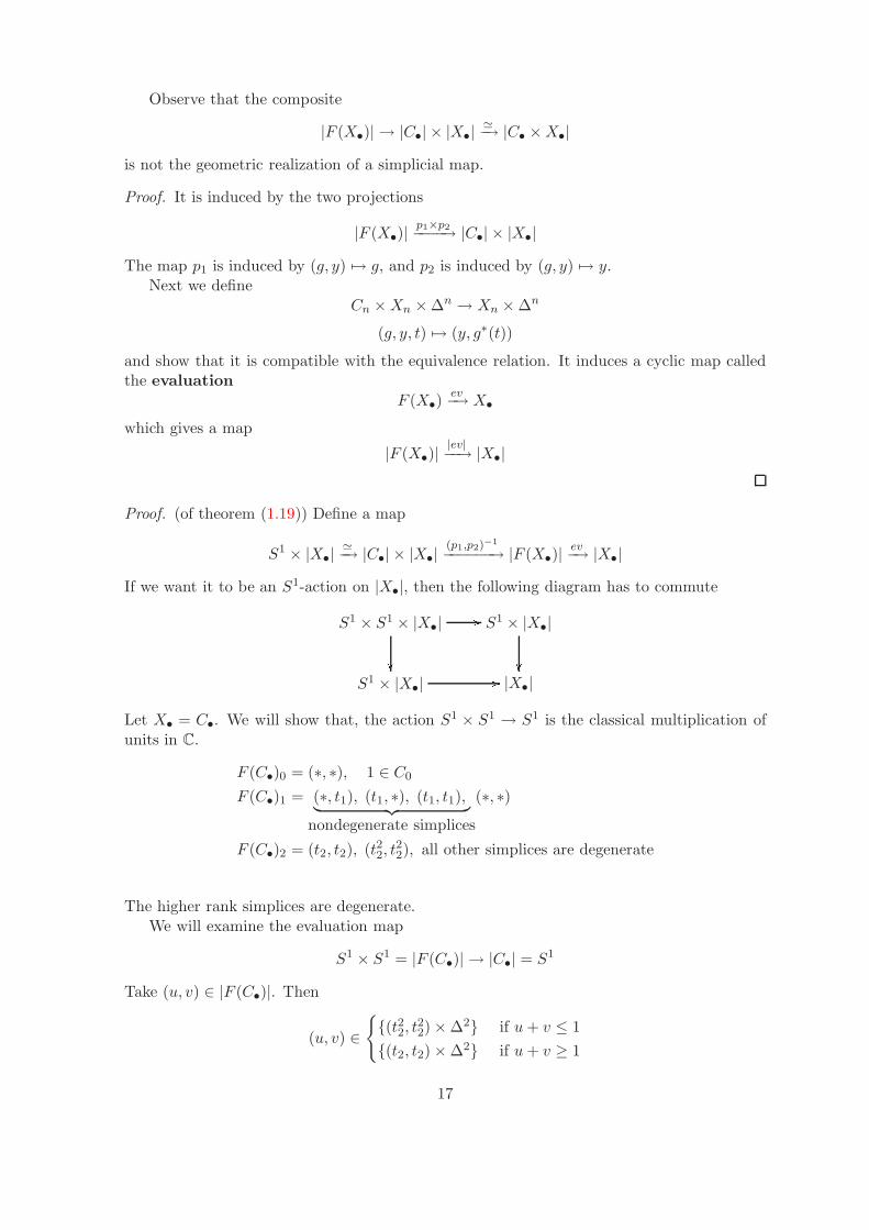
Observe that the composite

|F (X•)| → |C•| × |X•|≃−→ |C• ×X•|

is not the geometric realization of a simplicial map.

Proof. It is induced by the two projections

|F (X•)|p1×p2−−−−→ |C•| × |X•|

The map p1 is induced by (g, y) 7→ g, and p2 is induced by (g, y) 7→ y.Next we define

Cn ×Xn ×∆n → Xn ×∆n

(g, y, t) 7→ (y, g∗(t))

and show that it is compatible with the equivalence relation. It induces a cyclic map calledthe evaluation

F (X•)ev−→ X•

which gives a map

|F (X•)||ev|−−→ |X•|

Proof. (of theorem (1.19)) Define a map

S1 × |X•|≃−→ |C•| × |X•|

(p1,p2)−1

−−−−−−→ |F (X•)|ev−→ |X•|

If we want it to be an S1-action on |X•|, then the following diagram has to commute

S1 × S1 × |X•| // S1 × |X•|S1 × |X•| // |X•|

Let X• = C•. We will show that, the action S1 × S1 → S1 is the classical multiplication ofunits in C.

F (C•)0 = (∗, ∗), 1 ∈ C0

F (C•)1 = (∗, t1), (t1, ∗), (t1, t1),︸ ︷︷ ︸nondegenerate simplices

(∗, ∗)

F (C•)2 = (t2, t2), (t22, t22), all other simplices are degenerate

The higher rank simplices are degenerate.We will examine the evaluation map

S1 × S1 = |F (C•)| → |C•| = S1

Take (u, v) ∈ |F (C•)|. Then

(u, v) ∈

(t22, t

22)×∆2 if u+ v ≤ 1

(t2, t2)×∆2 if u+ v ≥ 1

17

The formulas

d0(t2, t2) = (∗, t1)

d2(t22, t

22) = (t1, ∗)

show that the 0-th face of the triangle (t2, t2) has to be identified with the 2-nd face of thetriangle (t22, t

22).

(*,t )1

(*,t )1

(t ,* )1(t ,* )1

(t ,t )2 222

(t ,t )22

1 1(t , t )

(*,*)

(*,*)

(*,*)

(*,*)

Figure 1.9: 0,1, and 2-faces

F (C•)ev−→ C•, (t2, t2) 7→ t2

ev(t22, t22) = t42 = t2 = s1(t1), because t32 = 1

ev(t2, t2) = t22 = s0(t1)

F (C•)|ev| ##GGGGGGGGp1×p2xxrrrrrrrrrr

|C•| × |C•| // |C•|

S1 × |C•| → |C•|

C0 = 1

C1 = 1, t1

C2 = 1, t2, t22

Degenerate simplices will be identified with the interval. There are two ways to do that.

⋃n≥0 F (C•)×∆n // ⋃

n≥0Cn ×∆n|F (C•)| // |C•|

ev : (t2, t2)×∆2 7→ (s0t1,∆2)

ev : (t22, t22)×∆2 7→ (s1t1,∆

2)

Therefore the map |ev| : S1 × S1 → S1 is the multiplication of complex units (under theexponential map exp(2πi−) : R/Z→ SO(2)).

18

u

2

0

(t , t )22 2

2

u+v

|ev|

s1

v

1

Figure 1.10:

(t , t )2 2

|ev|

u

v

21 s

0

0

u+v

Figure 1.11:

At the end we get a commutative diagram:

S1 × S1 × |X•| //

S1 × |X•|

F (C•)× |X•|

llXXXXXXXXXXXXXXXXXXXXXXXX 33hhhhhhhhhhhhhhhhhhhh|C•| × F (X•)

aaDDDDDDDDDDDDDDDDDDDDDzzzzzzzzzzzzzzzzzzz

z |F (F (X•))| //oo OO |F (X•)|

AA;;;;;;;;;;;;;;;;

;;|F (X•|rrffffffffffffffffffffffffffffff ++VVVVVVVVVVVVVVVVVVVVVVVVV

S1 × |X•| // |X•|

As a consequence |X•| is an S1-space.

19

1.8 Simplicial modules

Definition 1.24. A simplicial module is a functor

∆op →Modk, [n] 7→Mn

There is a chain complex associated to a simplicial module

M• : . . .→Mnbn−→Mn−1

bn−1−−−→Mn−1 → . . .

where b = bn =∑n

i=0(−1)idi. We have b2 = 0 as an immediate consequence of didj = dj−1di,i < j, for example:

. . .M2d0−d1+d2−−−−−−→M1

d0−d1−−−−→M0

(d0 − d1)(d0 − d1 + d2) = d0d0 − d0d1︸ ︷︷ ︸0

+ d0d2 − d1d0︸ ︷︷ ︸0

+ d1d1 − d1d2︸ ︷︷ ︸0

= 0

We define the homology of a simplicial module as

Hn(M•) := ker(bn)/ im(bn−1)

It is well defined for presimplicial module, that is using only face maps.

Lemma 1.25. The submodule M ′n of Mn spanned be the degeneracy elements gives a sub-

complex M ′• of M•.

Proof. This is a consequence of the relations between sj, di.

Define the normalized complex M• as a quotient

0→M ′• →M• →M• → 0

Theorem 1.26. The quotient map M• → M• is an quasi-isomorphism, i.e. it induces anisomorphism in homology.

Proof. From the long exact sequence in homology

. . .→ Hn(M′•)→ Hn(M•)→ Hn(M •)

δ−→ Hn−1(M

′•)→ . . .

it is enough to prove that Hn(M′•) = 0.

If one wants to prove that some complex C• is acyclic, then it is enough to construct ahomotopy from id to 0 (contraction), that it a sequence of maps hn : Cn → Cn+1 such thathn−1dn−1 + dnhn = id. Unfortunately it is hard to find a contracting homotopy for M ′

• toprove that it is acyclic. But one can define a filtration on M ′

•

Fk → Fk+1 → Gk

with Fk spanned by the first k degeneracies, and quotient G• for which we can construct acontracting homotopy. Then we can proceed by induction.

Let A be a k-algebra and M an A-module. There is a simplicial module

C•(A,M) := M ⊗A⊗n

20

di(a0, a1, . . . , an) = (a0, . . . , aiai+1, . . . , an), i = 0, . . . , n− 1

dn(a0, a1, . . . , an) = (ana0, . . . , an−1)

sj(a0, a1, . . . , an) = (a0, . . . , aj , 1, aj+1, . . . , an)

Define

b :=

n∑

i=0

(−1)idi

Then (C•(A,M), b) is called the Hochschild chain complex, and its homology H∗(A;M)the Hochschild homology of A with coefficients in M . If M = A, then we denote

H∗(A;A) =: HH∗(A)

Suppose that A is augmented and let A be its augmentation ideal in A, that is A = A⊕ k1.Define the reduced Hochschild complex as

Cn(A,M) := M ⊗A⊗n

If M = A = A⊕ k1, then C•(A,A) has extra degeneracy

s−1(a0, . . . , an) = (1, a0, . . . , an).

We have

d0(1, a1, . . . , an) = (a1, . . . , an)

dn(1, a1, . . . , an) = (an, . . . , a1)

Define also two maps on A⊗n

t(a1, . . . , an) := (−1)n(an, a1, . . . , an−1)

b′ :=

n−1∑

i=0

(−1)idi, (b = b′ + (−1)ndn)

1.9 Bicomplexes

Assume we have an array of k-modules

... ... ...C02

dv C12dhoo

dv C22dhoo

dv . . .ooC01

dv C11dhoo

dv C21dhoo

dv . . .ooC00 C10

dhoo C20dhoo . . .oo

21

We call it a bicomplex of k-modules if the maps dv and dh, called vertical and horizontaldifferential, satisfy

dv dv = 0

dh dh = 0

dh dv + dv dh = 0

For a bicomplex C•• we define a total complex as

Tot(C••)n :=⊕

p+q=n

Cpq, d := dh + dv

After taking homology with respect to the vertical differential we obtain a complex

. . .← Hv(p−1),• ← Hv

p,• ← Hv(p+1),• ← . . .

with the differential induced on homology by horizontal differential in the bicomplex. Nowwe can take homology of this complex and obtain

E2pq := Hh

q (Hvp,•)

There is a decomposition of the reduced Hochschild complex

Cn(A,A) = A⊗A⊗n

= (A⊕ k1)⊗A⊗n

= A⊗(n+1)

⊕A⊗n

and a map (b 1− t0 −b′

): A

⊗(n+1)⊕A

⊗n→ A

⊗n⊕A

⊗(n−1)

which fits in the diagram

Cn(A,A)

b ≃ //A

⊗(n+1)⊕A

⊗n0

@

b 1− t0 −b′

1

ACn−1(A,A)

≃ //A

⊗n⊕A

⊗(n−1)

This complex can be thought of as the total complex of a bicomplex

... ...A

⊗3

b A⊗31−too

−b′ A

⊗2

b A⊗21−too

−b′ A A

1−tooHere we see the beginning of the complex computing the homology of the cyclic group withcoefficients in a module. This will lead to the cyclic bicomplex.

22

1.10 Spectral sequences

Having computed E2pq = Hh

q (Hvp,•) of a bicomplex C•• it seems that we have used all data,

that is vertical and horizontal differentials in the bicomplex. However, there is a piece ofinformation which we can extract in addition to E2

pq. We can define a homomorphism

d2 : E2pq → E2

p−2,q+1

as follows.

Cp−2,q+1 Cp−1,q+1dhoo

dv Cp−1,q Cpq

dhooUsing a horizontal cycle x ∈ Zp(C•,q) we want to define an element in Cp−2,q−1 which repre-sents an element in horizontal cycles of vertical homology complex, that is in Zhp(H

vq(C••)).

Our x gives [x] ∈ Hvq(C••). Using the induced map

dh∗ : Hvq(Cp,•)→ Hv

q(Cp−1,•)

we have dh∗([x]) = 0 = [dh(x)]. Saying that the homology class is zero means that the cycleis in fact a boundary. Therefore there exists an y ∈ Cp−1,q+1 such that dv(y) = dh(x). Nowwe define our cycle as dh(y) ∈ Cp−2,q+1.

dh(y) ydhoo

dv dv(y) = dh(x) xdhoo

We claim that this element defines an element in E2p−2,q+1 which does not depend on the

choice of y nor on the choice of the representative of [x]. Thus we have defined

d2 : E2pq → E2

p−2,q+1, [x] 7→ [dh(y)].

Furthermore d2 d2 = 0, so now we can take homology to obtain E3pq and

d3 : E2pq → E3

p−3,q+2.

This procedure can be continued and as a result we get a sequence of arrays Erpq for any r ≥ 2and maps

dr : Erpq → Erp−r,q+r−1

such that Erpq is the homology of the complex (Er−1, dr−1) at the place (p, q). Furthermorethere are subspaces Br

pq, Zrpq of Cpq

B2pq ⊆ B

3pq ⊆ . . . ⊆ B

∞pq ⊆ Z

∞pq ⊆ . . . ⊆ Z

2pq ⊆ Z

2pq ⊆ Cpq

23

such that Erpq = Zrpq/Brpq.

• • • • • • • •

• • • • • • • •

• • • • • • • •

• • • • • • • •

• • • • •

ggOOOOOOOOOOOOOOeeJJJJJJJJJJJJJJJJJJJJJJJ

GGGGGGGGGGGGGGGGGGGGGGGGGGGGGGGGG• • •

• • • • • • •

ggOOOOOOOOOOOOOO•

• • • • • • • •

eeJJJJJJJJJJJJJJJJJJJJJJJ• • • • • • • •

q

OO

p//

When both differentials (leaving and entering) for Erpq are zero, this component does notchange furthermore and we have Erpq = Er+1

pq = . . .. We denote this stable component byE∞pq .

There is a filtration on the total complex

Fp TotC•• := Tot⊕

k≤p

Ck•,

0 ⊆ F0 ⊆ F1 ⊆ . . . ⊆ Fp−1 ⊆ Fp ⊆ . . . ⊆ TotC••.

This filtration induces a filtration on H∗(TotC••)

Fp := Fp H∗(TotC••) := im(H∗(Fp TotC••)→ H∗(TotC••))

Denote the quotientFp/Fp−1 =: grp(Hp+q(TotC••)).

All data defined above, that is Erpq, drp,q,r and a filtration Fpp define a spectral sequence

of a bicomplex C••. We say that the spectral sequence abuts to H∗(TotC••), which meansthat there is an isomorphism

E∞pq ≃ grp(Hp+q(TotC••))

We writeE2pq = Hh

p(Hvq(C••)) =⇒ Hp+q(TotC••).

which is to be read as: there is a spectral sequence starting at E2pq and converging to

Hp+q(TotC••)

24

Example 1.27. The typical theorem using spectral sequences in algebraic topology looks asfollows

Theorem 1.28. Let F → E → B be a fibration of connected spaces, with B simply connected.Then there is a spectral sequence

E2pq = Hp(B; Hq(F )) =⇒ Hp+q(E).

The implicit data in this theorem are E3pq, E

4pq, . . ., the filtration Fp on H∗(E). The sign

” =⇒ ” means that there is an isomorphism

E∞pq ≃ grp(Hp+q(E)).

In many cases we do not need to look at Erpq for r ≥ 3 and at the filtration. That is whythese data are often omitted in the theorems.

Example 1.29. Let X be an S1-space, ES1 contractible space of paths on S1. Consider theBorel space ES1 ×S1 X an S1-fibration

S1 → ES1 ×S1 X → X.

The homology of the fiber is

H0(S1) = Z,

H1(S1) = Z,

Hq(S1) = 0, q ≥ 2.

E2 : . . . . . . . . . . . . . . . . . .

0 0 0 0 0 0

• • • • • •

• • •

hhRRRRRRRRRRRRRRRR•

hhRRRRRRRRRRRRRRRR•

hhRRRRRRRRRRRRRRRR•

hhRRRRRRRRRRRRRRRRq

OOp

//E3 = . . . = E∞ : . . . . . . . . . . . . . . . . . .

0 0 0 0 0 0

• • • E2pq/ im d2 •

• • • • • •

q

OOp

//25

For any S1-fibration S1 → Ef−→ B of pointed spaces we obtain a Gysin sequence

. . .→ Hn(E)f∗−→ Hn(B)

d2−→ Hn−2(B)→ Hn−1(E)→ . . . .

Recall that for the bicomplex we took the vertical homology and then horizontal homology.We could have done it the other way. Any bicomplex gives a rise to two spectral sequences

E′2pq = Hh

p(Hvq(C••)) =⇒ Hp+q(Tot(C••))

E′′2pq = Hv

p(Hhq (C••)) =⇒ Hp+q(Tot(C••))

But remark that the filtrations are different on Tot(C••).

26

Chapter 2

Cyclic homology

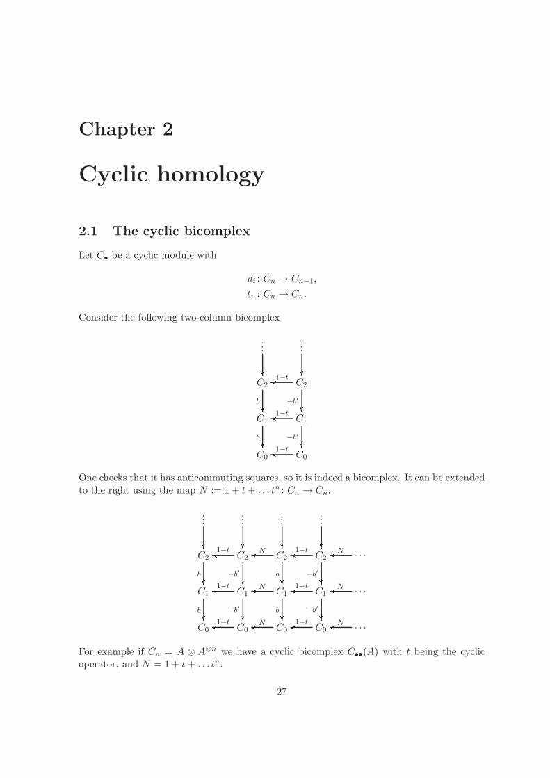
2.1 The cyclic bicomplex

Let C• be a cyclic module with

di : Cn → Cn−1,

tn : Cn → Cn.

Consider the following two-column bicomplex

... ...C2

b C2

−b′ 1−tooC1

b C1

−b′ 1−tooC0 C0

1−tooOne checks that it has anticommuting squares, so it is indeed a bicomplex. It can be extendedto the right using the map N := 1 + t+ . . . tn : Cn → Cn.

... ... ... ...C2

b C2

−b′ 1−too C2

b Noo C2

−b′ 1−too . . .NooC1

b C1

−b′ 1−too C1

b Noo C1

−b′ 1−too . . .NooC0 C0

1−too C0Noo C0

1−too . . .NooFor example if Cn = A ⊗ A⊗n we have a cyclic bicomplex C••(A) with t being the cyclicoperator, and N = 1 + t+ . . . tn.

27

Definition 2.1. The cyclic homology of a cyclic module C• is defined as

HCn(C•) := Hn(Tot(C••)).

When Cn = A⊗A⊗n then the cyclic homology of an algebra A is denoted by HCn(A).

Proposition 2.2. The complex (C•, b′) is acyclic.

Proof. Use extra degeneracy

(a0, . . . , an) 7→ (1, a0, . . . , an)

to construct a homotopy of the identity and the zero map.

Whenever we have a sequence of complexes

K ′• K• ։ K ′′

•

and we know that K ′• is acyclic, then the complexes K• and K ′′

• are quasi-isomorphic. Thisallows us to quotient out the acyclic subcomplexes of a given complex when computinghomology. But (C•,−b

′) is not a subcomplex. We will get rid of one column at a time using

Lemma 2.3 (Killing contractible complexes). Suppose we have o complex

. . .→ An ⊕A′n

d=

0

@

α βγ δ

1

A

−−−−−−−−→ An−1 ⊕A′n−1 → . . .

and (A′•, δ) has a homotopy h between id and 0. Then the following inclusion is a quasi-

isomorphism

(A•, α − βhγ)(id,−hγ)−−−−−→ (A• ⊕A

′•, d).

The cokernel of (id,−hγ) is (A′•, δ). Applied infinitely many times to the cyclic bicomplex

we end up with the total complex of the bicomplex B•C•

... ... ...C2

b C2

b B

ffLLLLLLLLLLLLLLC2

b B

ffLLLLLLLLLLLLLL. . .

C1

b C1

b B

ffNNNNNNNNNNNNNC1

b B

ffNNNNNNNNNNNNN. . .

ffNNNNNNNNNNNNNC0 C0

B

ffNNNNNNNNNNNNNC0

B

ffNNNNNNNNNNNNN. . .

ffNNNNNNNNNNNNNThis is the normalized version of the bicomplex C•• used to define cyclic homology. Becauseof the quasi-isomorphism in the lemma (2.3) we have

H∗(C•) = H∗(Tot(B•C•)).

28

We can rearrange the bicomplex B•C• to obtain

... ... ... ...

C2

b C1

b Boo C0Boo

C1

b C0Boo

C0

It is indeed a bicomplex, that is we have the identities

b2 = 0, B2 = 0, bB +Bb = 0.

The morphism B on the normalized complex B•C•(A) is given explicitly by

B = (1− t)sN : A⊗A⊗n→ A⊗A

⊗(n+1),

(a0, . . . , an) 7→

n∑

i=0

(−1)in(1, ai, . . . , an, a0, . . . , an−1).

In the non-normalized complex there are more terms, but they are trivial in the normalizedcomplex.

Theorem 2.4. For a cyclic module C• there exits a periodicity exact sequence

. . .→ Hn(C•)I−→ HCn(C•)

S−→ HCn−2(C•)

B−→ Hn−1(C•)→ . . . , (2.1)

where the map I is induced by the inclusion of the simplicial complex for C• into bicomplexC••.

If Cn = A⊗n the sequence takes the form

. . .→ HHn(A)I−→ HCn(A)

S−→ HCn−2(A)

B−→ HHn−1(A)→ . . . . (2.2)

Proof. It follows from the bicomplex (B•C•, b, B) and the sequence of complexes

C• Tot(B•C•) ։ TotB•C•[−2].

Prove that the boundary map is given by B. Find an explicit formula for S.

2.2 Characteristic 0 case

Recall the computation of the homology of the cyclic group Z/nZ. Let M be a module overZ/nZ, that is a module over the group ring k[Z/nZ] for some ring k. to compute Hi(Z/nZ;M)one uses the complex

M1−t←−−M

N←−M

1−t←−−M

N←− . . .

When the ring k is a field of characteristic 0, there is a homotopy from id to 0,

Mh−→M

h′−→M

h−→M

h′−→ . . . ,

29

h := −1

n

n−1∑

i=1

iti,

h′ :=1

nid,

h(1 − t) +Nh′ = tn = id.

It proves that

H0(Z/nZ;M) = M/1− t,

Hn(Z/nZ;M) = 0, n ≥ 1.

Now instead of considering the bicomplex C•• we can take the reduced complex Cλ• which isdefined as a cokernel of the map (1− t) between first and zeroth column of C••

... ...

C3/(1 − t)

b 0

C2/(1 − t)

b 0

C1/(1 − t)

b 0

C0/(1 − t) 0

If Cn = A⊗(n+1), then Cλn(A) = A⊗(n+1)/(1 − t) and we denote

Hλn(A) := Hn(C

λ• )

As a corollary we have that if k ⊃ Q, then Hλ(A) ≃ HCn(A) and there exists an exactsequence

. . .→ HHn(A)I−→ Hλ

n(A)S−→ Hλ

n−2(A)B−→ HHn−1(A)→ . . . .

In the case of characteristic not equal 0 the maps are still defined, but the sequence is notexact.

2.3 Computations

Let A = k, the ground ring. Then

HH0(k) = k,

HHn(k) = 0, n ≥ 1.

The periodicity exact sequence (2.2) implies that

HC2n(k) = k,

HC2n+1(k) = 0,

30

so also

Hλ2n(k) = k,

Hλ2n+1(k) = 0.

Let A = T (V ) be the tensor algebra over V , that is

T (V ) =

∞⊕

n=0

V ⊗n, (v1, . . . , vn)(vn+1, . . . , vn+m) = (v1, . . . , vn+m) ∈ V ⊗(n+m)

Then

HH0(T (V )) =⊕

m≥0

V ⊗m/(1 − τ) =⊕

m≥0

(V ⊗m)Z/mZ,

HH1(T (V )) =⊕

m≥0

(V ⊗m)Z/mZ,

HH1(T (V )) = 0,

where τ is the cyclic operator without sign.

HCn(T (V )) = HCn(k)⊕⊕

m>0

Hn(Z/mZ;V ⊗m)

︸ ︷︷ ︸This is zero in the characteristic 0 case.

Consider now the matrix algebra Mn(A) for a unital associative algebra A over a field k.There are isomorphisms

HH∗(Mr(A)) ≃ HH∗(A),

HC∗(Mr(A)) ≃ HC∗(A).

The map A→Mr(A) is given by

a 7→

(a 00 0

).

In the opposite way Tr: Mr(A)→ A we have the trace map

α = [αij ] 7→∑

i

αii.

There is also a trace map Tr: Mr(A)⊗(n+1) → A⊗(n+1)

Tr(α0, . . . , αn) :=∑

(i0,...,in)

α0i0i1 ⊗ α

1i1i2 ⊗ . . . ⊗ α

nini0

called the Dennis trace map. We claim that this map commutes with the faces and withthe cyclic operator.

Let k be a field and A a commutative k-algebra. Define the space of 1-forms on A, denotedby Ω1

A/k = Ω1A, as an A-module generated by elements da for every a ∈ A satisfying following

relations

d(λa+ µb) = λda+ µdb (linearity),

d(ab) = adb+ bda (Leibniz rule).

31

Define the space of n-forms as an n-th exterior power of Ω1A

ΩnA := ΛnAΩ1

A.

Elements of ΩnA can be written as a0da1 . . . dan, ai ∈ A, i = 0, . . . , n, with the relation

dada′ = −da′da.

Define a differential of an n-form as

d(a0da1 . . . dan) := 1da0da1 . . . dan.

d : ΩnA → Ωn+1

A , d d = 0.

Now Ω•A is a cochain complex and its homology is called deRham cohomology of the algebra

AHdR(A) := Hn(Ω

•A, d).

If A is commutative, M an A-module, then

H1(A;M) = M ⊗A Ω1A.

There is a map

π : Cn(A) = A⊗(n+1) → ΩnA

(a0, . . . , an) 7→ a0da1 . . . dan (2.3)

There is a map also in the opposite way

ΩnA

εn−→ HHn(A)

εn(a0da1 . . . dan) :=∑

σ∈Sn

sign(σ)(a0, aσ(1), . . . , aσ(n)). (2.4)

Passing to Hochschild homology it gives a well defined map ΩnA → HHn(A). In charecteristic

0 case the composition of the maps in (2.4) and (2.3) gives an isomorphism

ΩnA → HHn(A)→ Ωn

A.

Proposition 2.5. The following diagram is commutative

ΩnA

εn //d HHn(A)

BΩn+1A

εn+1 // HHn+1(A)

Proof. There is a bijection of sets Sn+1 ≃ Sn×Z/(n+1)Z. First one proves the commutativityof the following diagram

A⊗ ΛnAεn // Cn(A)

A⊗ Λn+1Aεn+1 // Cn+1(A)

and then passes to the quotient.

32

Now we can form a map of bicomplexes

... ... ... ...

C2

b C1

b Boo C0Boo

C1

b C0Boo

C0

π∗−→ ... ... ... ...

Ω2

0 Ω1

0 doo Ω0dooΩ1

0 Ω0dooΩ0

Definition 2.6. A commutative algebra A is formally smooth if for any commutativealgebra R and two sided ideal R ⊃ I such that I2 = 0 and a map A→ R/I, there is a liftingϕ : A→ R.

RA

ϕ==|||||||| // R/I

Theorem 2.7 (Hochschild-Kostant-Rosenberg). If A is formally smooth, then

ε∗ : M ⊗A ΩnA → H∗(A;M)

is an isomorphism.

As a corollary we have that for a formally smooth algebra A over characteristic 0 field k

HCn(A) ≃ ΩnA/dΩ

n−1A ⊕HdR

n−2(A)⊕HdRn−4(A)⊕ . . .⊕HdR

0(A) or HdR1(A).

2.4 Periodic and negative cyclic homology

Recall the cyclic bicomplex

... ... ... ...

C2

b C1

b Boo C0Boo

C1

b C0Boo

C0

33

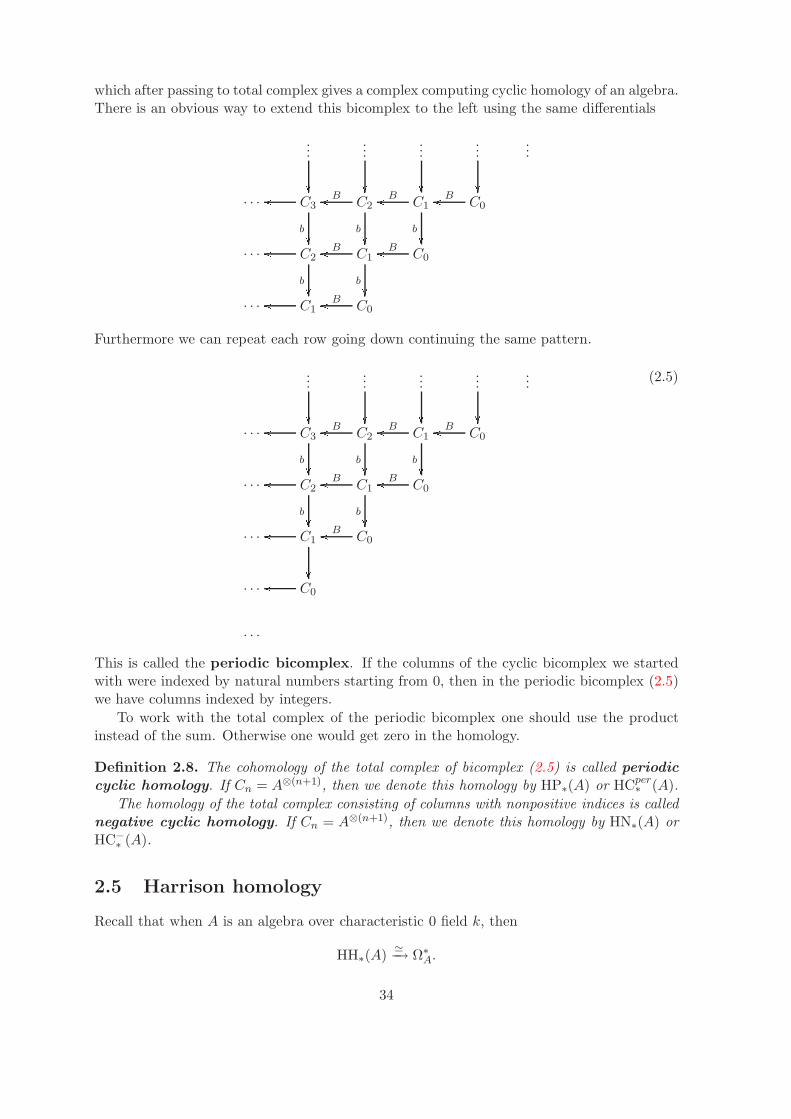
which after passing to total complex gives a complex computing cyclic homology of an algebra.There is an obvious way to extend this bicomplex to the left using the same differentials

... ... ... ... ...

. . . C3

b oo C2

b Boo C1

b Boo C0Boo

. . . C2

b oo C1

b Boo C0Boo

. . . C1oo C0

BooFurthermore we can repeat each row going down continuing the same pattern.

... ... ... ... ...

. . . C3

b oo C2

b Boo C1

b Boo C0Boo

. . . C2

b oo C1

b Boo C0Boo

. . . C1oo C0

Boo. . . C0

oo. . .

(2.5)

This is called the periodic bicomplex. If the columns of the cyclic bicomplex we startedwith were indexed by natural numbers starting from 0, then in the periodic bicomplex (2.5)we have columns indexed by integers.

To work with the total complex of the periodic bicomplex one should use the productinstead of the sum. Otherwise one would get zero in the homology.

Definition 2.8. The cohomology of the total complex of bicomplex (2.5) is called periodic

cyclic homology. If Cn = A⊗(n+1), then we denote this homology by HP∗(A) or HCper∗ (A).

The homology of the total complex consisting of columns with nonpositive indices is callednegative cyclic homology. If Cn = A⊗(n+1), then we denote this homology by HN∗(A) orHC−

∗ (A).

2.5 Harrison homology

Recall that when A is an algebra over characteristic 0 field k, then

HH∗(A)≃−→ Ω∗

A.

34

In general there is a decomposition into direct sum

HHn(A) = ⊕ . . .⊕︸ ︷︷ ︸n terms

⊕ΩnA

. . .

HH2(A) = ⊕ Ω2A

HH1(A) =

When one considers the first summands in each gradation then what one obtains is calledHarrison homology of the algebra A. When M is an A-bimodule, then Cn(A,M) =M⊗AA

⊗n gives a complex computing Hochschild homology of the algebra A with coefficientsin M . The complex for Harrison homology we obtain by taking a quotient by the shuffles inCn(A,M).

2.6 Derived functors

The Hochschild homology of an algebra A over a field k with coefficients in an A-bimoduleM can be interpreted as a derived functor

Proposition 2.9. There is an isomorphism

Hn(A;M) ≃ TorAe

n (M,A),

where Ae = A⊗Aop (so M is a right Ae-module).

The definition of the derived functor TorAe

n goes as follows. Having an exact sequence ofright Ae-modules

0→M ′ →M →M ′′ → 0

we tensor it with A over Ae to get a sequence which is exact on the right

M ′ ⊗Ae A→M ⊗Ae A→M ′′ ⊗Ae A→ 0,

but the mapM ′⊗AeA→M⊗Ae can have a nontrivial kernel, which we define as TorAe

1 (M ′′, A).Next we can define in an analogous way TorA

e

1 (M,A) and TorAe

1 (M ′, A) which fit into an exactsequence

TorAe

1 (M ′, A)→ TorAe

1 (M,A)→ TorAe

1 (M ′, A)→M ′ ⊗Ae A→M ⊗Ae A→M ′′ ⊗Ae A→ 0.

General construction uses a resolution of A by free left Ae-modules, C• ։ A→ 0,

. . . // C2// C1

// C0A0

Then we define

TorAe

n (M,A) := Hn(M ⊗Ae C•).

35

As a resolution we can take Cn := Ae ⊗ A⊗n and obtain the isomorphism Hn(A,M) ≃TorA

e

n (M,A).Recall that the simplicial module C• is a functor ∆op →Mod, for example [n] 7→M ⊗Ae

An. The homology of C• with respect to b =∑

i(−1)idi can be written as a derived functor

Hn(C•) ≃ Tor∆op

n (k,C•),

where C• is a left module over ∆op, and k is a right module over ∆op, that is a functor∆→Mod, [n] 7→ k. The resolution for k can be given by

. . . // k[Hom∆([n],−)] // . . . // k[Hom∆([1],−)] // k[Hom∆([0],−)]k

In general for a category C we have the following correspondence

Category C Algebra A

Functor F : C →Mod Left A-module MFunctor G : Cop →Mod Right A-module N

Tensor product over a category G⊗C F Tensor product over algebra N ⊗AM

The tensor product over a category is defined as

G⊗C F :=⊕

C∈Ob(C)

G(C)⊗ F (C)/ ∼,

where the equivalence relation ∼ is given by

y ⊗ f∗(x) ∼ f∗(y)⊗ x, C

f−→ D, x ∈ F (C), y ∈ G(D),

F (C)f∗−→ F (D), G(C)

f∗←− G(D).

Using cyclic category ∆C we can present cyclic homology of a cyclic module C• as a derivedfunctor.

Proposition 2.10. There is an isomorphism

HCn(C•) ≃ Tor∆Cop

n (k,C•).

We can write TorC0(G,F ) simply as the tensor product G⊗C F . To define higher derivedfunctors TorCn(G,F ) we need a notion of a free module over a category. Let Ctriv be thecategory with the same objects as C, but with only the identity morphisms. For a functorF : C → Mod there is a corresponding forgetful functor forget(F) : Ctriv → Mod. Supposewe have an adjoint pair

Funct(C,Mod)forgetful //

Funct(Ctriv,Mod)left adjoint

ooThen we say that a functor F : C →Mod is free if it is an image of this left adjoint functorto a forgetful functor. For example

A−Mod→ k −Mod

has a left adjointkn 7→ An.

36

Chapter 3

Relation with K-theory

We will define invariant of rings, called algebraic K-theory and denoted by K∗(A) for a ringA. Next we will describe its relation with cyclic homology by defining a map

K∗(A)→ HC∗(A).

3.1 K-theory

First we will define K-theory of a ring A in gradation 0, that is K0(A). We say that a finitelygenerated module over A is free if it is isomorphic to the product An for some n. A finitelygenerated A-module P is projective if it is a direct summand in a free A-module, that isthere exists an A-module Q such that P ⊕ Q ≃ An for some n. Such projective module Pcorresponds to idempotent in the matrix algebra Mn(A). The set of isomorphism classes offinitely generated projective modules over A is a monoid with respect to direct sum of classesdefined by

[P ] + [Q] =: [P ⊕Q].

There is an universal abelian group for this monoid (called the Grothendieck group), and wetake it as the definition of the K-theory of A, denoted by K0(A).

Let A be a commutative algebra over k. There exists a map

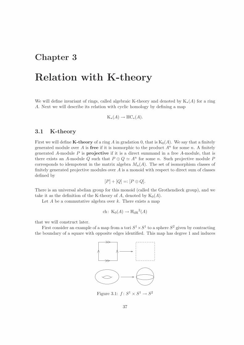
ch: K0(A)→ HdR2(A)

that we will construct later.

First consider an example of a map from a tori S1×S1 to a sphere S2 given by contractingthe boundary of a square with opposite edges identified. This map has degree 1 and induces

Figure 3.1: f : S1 × S1 → S2

37

an isomorphism

HdR2(S2)

deg(f)−−−−→ HdR

2(S1 × S1).

If we want to find an algebraic map of corresponding coordinate rings

S2a := C[X,Y,Z]/(X2 + Y 2 + Z2 − 1)→ C[U,U−1, V, V −1] =: (S1 × S1)a

then we will not succeed, because any algebraic map S1 × S1 → S2 is homotopic to theconstant map. The situation is very different now than it was in case of maps S3 → S2.Indeed, assume we have the map

f∗ : S2a → S1 × S1

a.

Then it induces a map on K-theory

K0(S2a)→ K0((S

1 × S1)a),

and we would have a commutative diagram

Z K0(S2a)

// K0((S1 × S1)a) 0

C HdR2(S2

a)deg(f)// HdR

2((S1 × S1)a) C

which gives a contradiction, because a generator of Z = K0(S2a) goes to generator of C =

HdR2(S2

a).Define a projector p and idempotent e in M2(S

2a) by the formulas

p :=

(X Y + iZ

Y − iZ −X

), p2 = 1, e :=

p+ 1

2, e2 = e.

Fact 3.1. The class of an image of e, [im e], generates K0(S2a).

Fact 3.2. For any ring A there is an isomorphism

K0(A[X,X−1]) ≃ K0(A).

3.2 Trace map

There is a trace map defined as

Tr: Mr(A)→ A, [aij]ri,j=1 7→

r∑

i=1

aii.

We can extend it to a mapTr: Mr(A)⊗(n+1) → A⊗(n+1),

[ai0j0]⊗ . . . ⊗ [ainjn ] 7→∑

k0,k1,...,kn

ak0k1 ⊗ ak1k2 ⊗ . . .⊗ aknk0

for any r ≥ 1, n ≥ 0. It induces a maps on Hochschild, cyclic, periodic cyclic and negativecyclic homology.

HHn(Mr(A))→ HHn(A), HCn(Mr(A))→ HCn(A), etc.

38

Let us take an idempotent e2 = e in Mr(A). Under the map b in Hochschild complex forMr(A) we have

e⊗(n+1) 7→

0 n even

e⊗n n odd

In Cλn(Mr(A)) we have e⊗(n+1) = (−1)ne⊗(n+1). If n is odd, then [e⊗(n+1)] = 0. If n = 2m iseven, then b[e⊗(n+1)] = 0, so [e⊗(n+1)] is a cycle, and we can define a map [e] 7→ [Tr(e⊗(n+1))],

K0(A)→ Hλ2m(M(A))

Tr−→ Hλ

2m(A),

M(A) =⋃

r

Mr(A), Mr(A) →Mr+1(A), α 7→

(α 00 0

).

We have to show that the element [Tr(e⊗(n+1))] ∈ Hλ2m(A) depends only on the isomorphism

class.

Lemma 3.3. An interior automorphism (conjugation) induces an identity for Hochschild,cyclic, periodic cyclic, negative cyclic homology.

We have constructed a functorial map K0(A)→ Hλ2m(A). Now we ask if we can construct

a map K0(A)→ HC2m(A)?Recall the cyclic bicomplex C••(A)

... ... ... ...C2

b C2

−b′ 1−too C2

b Noo C2

−b′ 1−too . . .NooC1

b C1

−b′ 1−too C1

b Noo C1

−b′ 1−too . . .NooC0 C0

1−too C0Noo C0

1−too . . .NooDefine

yi := (−1)i(2i)!

i!Tr(e⊗(2i+1)),

zi := (−1)i−1 (2i)!

2(i!)Tr(e⊗(2i)).

Proposition 3.4. The element ch([e]) := (ym, zm, ym−1, zm−1, . . . , y0, z0) ∈ (Tot(C••(A)))n,n = 2m+ 1 is a cycle. Furthermore the following diagram is commutative

K0(A)ch //ch &&MMMMMMMMMM ================

==Tr 44444444444444

444444444 HC2m(A)

SHC2m−2(A). . .

HC0(A)

39

For the bicomplex B•C• we have to use ch([e]) := (yn, yn−1, . . . , y0) ∈ (Tot(B•C•(A)))n.We can define a map

ch: K0(A)→ HdRev(A), ch([e]) := Tr(edede . . . de).

3.3 Algebraic K-theory

Let A be a ring with unit. Define a discrete group GL(A) as a direct limit of the groupsGLr(A) with respect to the maps

GLr(A) → GLr+1(A), α 7→

(α 00 1

).

There is a classifying space BGL(A) with

π1(B GL(A)) = GL(A),

πn(B GL(A)) = 0, n 6= 1.

We can apply the Quillen’s plus construction to obtain a space BGL(A)+ with the followingthree properties

1. the fundamental group is an abelianization of GL(A),

π1(B GL(A)+) = GL(A)/[GL(A),GL(A)],

2. there is an isomorphism on homology Hi(B GL(A)) ≃ Hi(B GL(A)+),

3. there is an H-space structure on BGL(A)+.

Thus H∗(B GL(A)+) is a commutative, cocommutative (and connected) Hopf algebra.

Definition 3.5. Higher K-theory groups of A are defined as

Kn(A) := πn(B GL(A)+), n ≥ 1.

Prior to this definition there were defined K1, K2, K3. We will describe these earlierdefinitions.

The K1 group of a ring A was defined as an abelianization of GL(A),

K1(A) = GL(A)/[GL(A),GL(A)].

For example if A = F is a field, then K1(F ) = F×, the group of invertible elements in F .The determinant map det : GL(F ) → F× can be generalized to noncommutative rings bythe map GL(A)→ K1(A).

Denote by E(A) the group generated by elementary matrices eaij , where each eaij is anidentity matrix plus the matrix with only one nonzero entry equal a in i-th row and j-thcolumn. Then

[GL(A),GL(A)] = E(A).

The elementary matrices eaij satisfy the following relations

eaijebij = ea+bij ,

eaijebkl = ebkle

aij , for j 6= k, i 6= l,

eaijebjk = ebjke

abike

aij .

(3.1)

40

The group E(A) can be presented using generators eaij which satisfy the relations (3.1) aboveplus some relations which depend on A. Define the Steinberg group St(A) of A as thegroup with the set of generators xaij with the relations (3.1). There is an epimorphismSt(A) ։ E(A) and we define K2(A) as the kernel of this map. Then K2(A) is abelian, andthe sequence

K2(A) St(A) ։ E(A)

can be shown to be a central extension.

Theorem 3.6 (Whitehead-Kervaire). The group E(A) is perfect, that is

H1(E(A)) = 0,

and

H2(E(A)) ≃ K2(A).

Proof. The proof relies on the spectral sequence of the fibration

B K2(A)→ B St(A)→ B E(A)

On the second table we have

E2pq = Hp(B E(A);Hq(B K2(A)))

and the sequence converges to Hp+q(St(A)). We have

Hp(BE(A);Hq(B K2(A))) ≃ Hp(E(A);Hq(K2(A))) ≃ Hp(E(A))⊗Hq(K2(A))

The second table looks like follows.

. . . 0 . . . . . . . . .

Λ2K2(A) 0 . . . . . . . . .

K2(A) 0 H2(E(A)⊗K2(A)

jjUUUUUUUUUUUUUUUUUH3(E(A)⊗K2(A) . . .

Z 0 H2(E(A))

jjUUUUUUUUUUUUUUUUUUH3(E(A))

llXXXXXXXXXXXXXXXXXXXXXXXXXXXXXXXXX. . . //

OO

41

One needs to prove that H2(St(A)) = 0, and that E∞pq looks like

0 0 • • . . .

0 0 • • . . .

Z 0 0 H3(St(A)) . . .

OO//

Theorem 3.7 (Gersten). There is an isomorphism

H3(St(A)) ≃ K3(A).

Proof. One has to prove that there is a fibration

BK2(A) // B St(A)+ // B E(A)+

BK2(A)+

and then use the above spectral sequence.

Summarizing earlier results we have

H1(GL(A)) = K1(A),

H2(E(A)) = K2(A),

H3(St(A)) = K3(A).

Let us look once more at the relations for the Steinberg group (3.1). We can label the edgesof the Stasheff polytope of dimension 2 as follows

•ebjk~~~~~~~ ea

ij•

eabik •

ebjk•

eaij

•

to encode the relation eaijebjk = ebjke

abike

aij . There is a way to put labels on the Stasheff polytope

of dimension 3 in the coherent way. It can be generalized to higher dimension.

42

Proposition 3.8 (Cartan). Let X be an H-space. Then

Prim H∗(X; Q) ≃ π∗(X)⊗Q

where the primitive elements of the Hopf algebra H are

Prim(H) := x ∈ H | ∆(x) = x⊗ 1 + 1⊗ x.

Corollary 3.9.

PrimH∗(GL(A); Q) ≃ K∗(A)⊗Q.

Let G = GLr(A). The map f : k[GLr(A)] → Mr(A) is the unique k-algebra map whichextends the inclusion of invertible matrices to matrices.

For any n there is defined a map of cyclic modules

k[Gn]ι−→ k[Gn+1] ≃ k[G]⊗(n+1) f⊗(n+1)

−−−−−→Mr(A)⊗(n+1) Tr−→ A⊗(n+2),

where ι(g1, . . . , gn) := ((g1 . . . gn)−1, g1, . . . , gn).

We can apply any of the cyclic theories HH, HC, HC−, HCper to this sequence to get, forinstance

H∗(GL(A))→ HC−∗ (A).

Working over Q and using collorary (3.9) we get the Chern character

ch : K∗(A)→ HC−∗ (A).

43