Embed Size (px)
Citation preview

This PDF is a selection from an out-of-print volume from the National Bureauof Economic Research
Volume Title: Currency Crises
Volume Author/Editor: Paul Krugman, editor
Volume Publisher: University of Chicago Press
Volume ISBN: 0-226-45462-2
Volume URL: http://www.nber.org/books/krug00-1
Publication Date: January 2000
Chapter Title: Current Account Reversals and Currency Crises: Empirical Regularities
Chapter Authors: Gian Maria Milesi Ferretti, Assaf Razin
Chapter URL: http://www.nber.org/chapters/c8695
Chapter pages in book: (p. 285 - 323)
urrent Account Reversals and Currency Crises Empirical Regularities
Gian Maria Milesi-Ferretti and Assaf Razin
8.1 Introduction
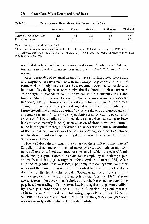
Three waves of external crises have swept international capital markets during the 1990s: the European Monetary System crisis in 1992-93, the collapse of the Mexican peso with its induced “tequila” effects, and, most recently, the financial crisis in East Asia. In Italy and Mexico, the currency crisis was followed by a sharp reversal in the current account; Italy went from a deficit of 2.4 percent in 1992 to an average surplus of close to 2 percent in 1993-96 and Mexico from a deficit of 7 percent in 1993-94 to virtual balance in 1995-96. A similar outcome has occurred in East Asia after the 1997 baht crisis and its aftermath, as table 8.1 shows.
Are external crises characterized by large nominal devaluations invari- ably followed by sharp reductions in current account deficits? And what is the impact of crises and reversals in current account imbalances on economic performance? Our paper addresses these questions by charac- terizing real and nominal aspects of sharp external adjustments in low- and middle-income countries. It presents stylized facts associated with sharp reductions in current account deficits (reversals) and with large
Gian Maria Milesi-Ferretti is senior economist in the Research Department of the Inter- national Monetary Fund and a research fellow of the Centre for Economic Policy Research, London. Assaf Razin is professor of economics at Tel Aviv University and Stanford Univer- sity and a research associate of the National Bureau of Economic Research.
The authors’ discussant, Jaume Ventura, and Enrica Detragiache, Pietro Garibaldi, Mi- chael Mussa, Eswar Prasad, conference participants, and IMF seminar participants gave useful comments. The authors are grateful to Andy Rose for sharing his STATA programs, and to Yael Edelman and especially Maria Costa for excellent research assistance. Work for the conference was supported in part by a grant to the NBER from the Center for Interna- tional Political Economy. The opinions expressed do not necessarily reflect those of the Inter- national Monetary Fund.
285
286 Gian Maria Milesi-Ferretti and Assaf Razin
Table 8.1 Current Account Reversals and Real Depreciation in Asia
Indonesia Korea Malaysia Philippines Thailand
Current account reversap 6.8 15.1 19.6 6.8 18.8 Real depreciationh 40.5 21.9 18.0 14.1 19.6
Source: International Monetary Fund. dDifference in the ratio of current account to GDP between 1998 and the average for 1995-97. ”Real effective exchange rate depreciation between July 1997-December 1998 and January 1995-June 1997 (period averages).
nominal devaluations (currency crises) and examines what pre-event fac- tors are associated with macroeconomic performance after such events occur.
Recent episodes of external instability have stimulated new theoretical and empirical research on crises, in an attempt to provide a conceptual framework that helps to elucidate these traumatic events and, possibly, to improve policy design so as to minimize the likelihood of their occurrence. In principle, a reversal in capital flows can cause a currency crisis and force a reduction in current account deficits because sources of external financing dry up. However, a reversal can also occur in response to a change in macroeconomic policy designed to forestall the possibility of future speculative attacks or capital flow reversals, or as a consequence of a favorable terms-of-trade shock. Speculative attacks leading to currency crises can follow a collapse in domestic asset markets (as seems to have been the case recently in Asia), accumulation of short-term debt denomi- nated in foreign currency, a persistent real appreciation and deterioration of the current account (as was the case in Mexico), or a political choice to abandon a rigid exchange rate system (as was the case in the United Kingdom in 1992).
How well does theory match the variety of these different experiences? So-called first-generation models of currency crises are built on an inevi- table collapse of a fixed exchange rate system, in which the central bank mechanically expands domestic credit, for example, by monetizing a per- sistent fiscal deficit (e.g., Krugman 1979; Flood and Garber 1984). After a period of gradual reserve losses, a perfectly foreseen speculative attack wipes out the remaining reserves of the central bank and forces the aban- donment of the fixed exchange rate. Second-generation models of cur- rency crises endogenize government policy (e.g., Obstfeld 1994). Private agents forecast the government’s choice as to whether or not to defend the peg, based on trading off short-term flexibility against long-term credibil- ity. The peg is abandoned either as a result of deteriorating fundamentals, as in first-generation models, or following a speculative attack driven by self-fulfilling expectations. Note that a self-fulfilling attack can (but need not) occur only with “vulnerable” fundamentals.
Current Account Reversals and Currency Crises 287
The latest waves of currency crises referred to above have brought ex- planations of crises based on multiple equilibria or on contagion effects to the forefront (on the former see, e.g., Eichengreen, Rose, and Wyplosz 1995; Jeanne and Masson 2000; among others; on the latter, Eichengreen et al. 1996; Calvo and Mendoza 1999; Jeanne 1997; Masson 1998)’ Em- pirical tests of crisis models use various indicators of fundamentals, such as the ratio of reserves to money, fiscal balance, and the rate of domestic credit creation. The issue is whether (some) fundamentals are steadily de- teriorating in the period leading up to a speculative attack or not. How- ever, it is difficult to infer from the data whether the collapse of the peg is a result of deteriorating fundamentals or self-fulfilling prophecies (see, e.g., Eichengreen et al. 1995; Krugman 1996). A growing body of research is devoted to studying the mechanics of crises in developing countries. Ed- wards (1989), who studied the link between devaluation, the current ac- count, and output behavior, is an important precursor of our work. Kamin- sky and Reinhart (1999), Kaminsky, Lizondo, and Reinhart (1998), and Demirguq-Kunt and Detragiache (1998) focus on leading indicators of balance-of-payments and banking crises; Sachs, Tornell, and Velasco (1996b) explore the spillover effects of the Mexican crisis on other emerging markets; closest to our work, Frankel and Rose (1996) undertake a cross- country study of currency crashes in low- and middle-income countries.
The focus of the literature on the intertemporal aspects of the current account goes back to work by Sachs (1981, 1982) and follows up on our own research on current account sustainability (Milesi-Ferretti and Razin 1996a, 1996b) and on current account reversals (Milesi-Ferretti and Razin 1998). Recent empirical research in the area includes Debelle and Faruqee (1996), who undertake a cross-country study of determinants of the cur- rent account, Kraay and Ventura (2000), who argue that debtor and credi- tor countries respond asymmetrically to income shocks, and Lane and Perotti (1998), who investigate the impact of fiscal policy on the trade bal- ance in OECD countries. A number of authors have instead focused on capital account developments, and in particular on capital flows to emerg- ing markets, underlining the importance of both “push” and “pull” factors in explaining capital flows (see, e.g., Calvo, Leiderman, and Reinhart 1993; Corbo and Hernandez 1996; Fernandez- Arias 1996; Fernandez- Arias and Montiel 1996).
In this paper we put together these related strands of literature and un- dertake a study of indicators and consequences of current account rever- sals and currency crises in a large sample of low- and middle-income coun- tries over the period 1970-96. We try to answer four questions: First, what
1. Contagion effects, broadly defined, can (but need not) have “fundamental” origins; e.g., a large depreciation in a country can imply a loss of competitiveness and a decline in external demand for a neighboring country. Eichengreen et al. (1996) try empirically to distinguish between different types of contagion.

288 Gian Maria Milesi-Ferretti and Assaf Razin
triggers large and persistent reductions in current account deficits? Sec- ond, what triggers sharp exchange rate depreciations (currency crises)? Third, what are the consequences of these events for output and consump- tion? Fourth, is there a link between current account reversals and cur- rency crises? Although our study does not focus directly on reversals in capital flows, it uses data on size and composition of external liabilities in its characterization of external crises, and it includes “push” factors, such as interest rates and economic growth in industrial countries, among fac- tors systematically associated with current account reversals and currency depreciation. Our findings concerning indicators of reversals and crises are in line with what is suggested by theoretical models, with both domes- tic factors (such as the level of reserves) and external factors (such as the terms of trade and world interest rates) playing a role in triggering rever- sals and crises. We also find that output performance before and after a currency crisis exhibits much more “continuity” than before and after a current account reversal, and that the majority of reversals are not pre- ceded or accompanied by a currency crisis.
In undertaking this empirical exercise, we attempt to characterize a broad set of stylized facts associated with reversals and crises. However, caution must be exercised in interpreting these regularities as a reliable predictive model. The burgeoning analytical literature on financial crises has highlighted several mechanisms that can generate such an outcome: inconsistency between deteriorating fundamentals and the maintenance of a fixed exchange rate (Krugman 1979), self-fulfilling crises a la Obstfeld (1994), and models of crises based on bank runs a la Diamond and Dybvig (1983) (Goldfajn and Valdes 1997; Chang and Velasco 1998). Although these mechanisms generating crises are different, the models point to an overlapping set of indicators (e.g., the level of reserves, the rate of growth in domestic credit, world interest rates, etc.). Hence empirical exercises relating the probability of a crisis to a large set of indicators cannot dis- criminate between different explanations for crises. Failure to identify the (potentially different) mechanisms underlying crises limits the usefulness of these exercises as predictive tools because the reduced-form relation between crisis events and indicators averages the particular pattern of cri- ses prevailing in the sample, which may not be repeated in the future (as in the standard Lucas critique). In addition, policy inference is hindered by the fact that the crisis-generating mechanisms, which we cannot disen- tangle, can have different policy implications (e.g., tight monetary policy is called for in a standard Krugman-type crisis, while a more flexible mon- etary policy is called for in the event of bank runs).
8.2 Theoretical Determinants of Reversals and Currency Crises
We can cast the analysis of sharp reversals in the current account in terms of the standard transfer problem, which is illustrated following

Current Account Reversals and Currency Crises 289
Krugman (1999). Consider a small open economy producing goods that are imperfect substitutes for traded goods produced abroad. Assume that the world marginal propensity to spend on the country’s product (set to zero for simplicity) is smaller than the country’s marginal propensity to spend on domestic goods, 1 - p . World demand for domestic exports is fixed at X . A share p of both consumption and investment demand (C and I ) falls on foreign goods. Market clearing for gross domestic product Y implies
Y 1 ( 1 - p ) I + (1 - p ) C + p x = (1 - k ) I + (1 - p)(l - s)Y + px, where s is the marginal propensity to save and p is the relative price of foreign goods in terms of domestic goods (a measure of the real exchange rate). For given Y and X it is possible to solve for p as a function of in- vestment:
Suppose that investment financing depends on external capital flows. A reversal in capital flows will cause a decline in investment and, for given output, a real depreciation. In terms of the transfer problem, the assump- tion that domestic residents have a higher marginal propensity to spend on domestic goods than do foreign residents implies that a transfer of resources from the home to the foreign country will increase world de- mand for foreign goods and decrease demand for domestic goods, thus implying the need for a real depreciation. To the extent that domestic out- put falls, this will mitigate the need for a real depreciation because of the induced fall in supply of domestic goods.
The first theoretical framework in which to describe currency crises was provided by Krugman (1 979) and Flood and Garber (1984). In this frame- work, the source of the crisis is an inconsistency between the exchange rate peg and the rate of domestic credit expansion that leads to a gradual depletion of foreign exchange reserves, culminating in a speculative attack in which the remaining reserves are wiped out instantly. The attack takes place once the “shadow exchange rate,” e’, defined as the implicit floating exchange rate that would prevail once reserves are exhausted, equals the pegged rate, e. In the simple monetary model on which this analysis is based, a measure of the vulnerability to speculative attacks is usefully given by
es - 1 - k(eRIM2) e
- - 1 - q7r
1
where p is the base money multiplier, M2 is broad money, R is the level of foreign exchange reserves, q is the interest semielasticity of the demand for money, and 7r is the rate of credit expansion. In this context, Calvo
290 Gian Maria Milesi-Ferretti and Assaf Razin
(1997) emphasizes the importance of the ratio eRIM2 and of the ratio of reserves to short-term debt as measures of the adequacy of international reserves. This class of models does not yield clear predictions with regard to the link between exchange rate crises and the behavior of the trade balance. However, if the model is amended to allow for capital controls (as in Wyplosz 1986) reserve depletion can take place through the current account as well, with trade deficits eventually leading to an exhaustion of reserves and a collapse of the peg.
Chang and Velasco (1998) provide a link between the literature on bank runs and the literature on international financial crises. A reduction in the availability of international liquidity can exacerbate the illiquidity of domestic banks, leading to a collapse in the banking system. This would cause an output decline and a collapse in asset prices. Under a fixed ex- change rate, a run on the banks becomes a run on the currency if the cen- tral bank attempts to act as a lender of last resort. For example, Korea’s banks had sizable short-term foreign currency liabilities and matching long-term foreign currency assets. At the beginning of the crisis foreign banks refused to roll over their short-term foreign currency assets vis-a- vis offshore and onshore Korean banks. The attempts by the central bank to shore up the foreign liquidity position of banks simply led to the rapid loss of foreign currency reserves and the collapse of the currency.
Insofar as current account reversals occur in periods of economic dis- tress, with liquidity constraints due to a reversal in capital flows, we would expect a link between reversals and large currency depreciations. However, this may not be the case when reversals are induced by other factors, such as favorable terms-of-trade developments. The empirical work of the next three sections characterizes empirical regularities associated with both current account reversals and currency crashes, attempts to shed light on what indicators provide a signal of the likelihood of these events oc- curring, and looks at whether reversals and currency crises are related.
8.3 The Data
Our data set consists of 105 low- and middle-income countries (48 Afri- can countries, 26 Asian countries, 26 countries from Latin America and the Caribbean, and 5 European countries). A complete list of countries is given in appendix A. In the empirical analysis we also make use of a re- duced sample, comprising 39 middle-income countries with population above one rnilliom2 These countries are indicated with an asterisk in ap- pendix A. The main source of data is the World Bank (World Tables and
2. These countries had income per capita (Summers and Heston definition) above $1,500 and population above one million in 1985, as well as an average current account deficit during the sample period below 10 percent of GDP.
Current Account Reversals and Currency Crises 291
World Development Indicators and Global Development Finance); appendix B describes data sources and definitions. In addition to standard macro- economic and external variables, the data set includes a number of finan- cial sector variables and variables reflecting the composition of external liabilities, whose role in determining the likelihood of external crises has been emphasized in the recent literature (see, e.g., Calvo 1997). The data belong to different categories:
Macroeconomic variables such as economic growth, real consumption growth, rate of investment, fiscal balance, and level of GDP per capita
External variables such as the current account balance (exclusive and in- clusive of official transfers), real effective exchange rate, degree of real exchange rate overvaluation,l degree of openness to trade, and level of external official transfers as a fraction of GDP
Debt variables such as the ratio of external debt to output; interest burden of debt as a fraction of GNP; shares of concessional debt, short-term debt; public debt, and multilateral debt in total debt; and ratio of FDI flows to debt outstanding
Financial variables such as the ratio of M2 to GDP, credit growth rate, and ratio of private credit to GDP
Foreign variables such as the real interest rate in the United States (as a proxy for world interest rates), rate of growth in OECD countries, and terms of trade4
Dummy variables such as regional dummies, a dummy for the exchange rate regime that takes the value one if the country’s exchange rate is pegged and zero otherwise, and a dummy that takes the value one if the country has an International Monetary Fund (IMF) program in place for at least six months during the year
8.4 Indicators of Current Account Reversals
In the definition of reversal events we want to capture large and persis- tent improvements in the current account balance that go beyond short- run current account fluctuations as a result of consumption smoothing. The underlying idea is that “large” events provide more information on determinants of reductions in current account deficits than short-run fluctuations. These events have to satisfy three requirements:
3. For the CPI-based real effective exchange rate (period average = loo), an increase repre- sents a real appreciation. The degree of real overvaluation, calculated using a bilateral rate vis-a-vis the U.S. dollar, is for every country the percentage deviation from the country’s sample average, as in Frankel and Rose (1996). Goldfajn and Valdes (1999) study the dynam- ics of real exchange rate appreciations and the probability of their “unwinding.” 4. For the terms-of-trade index, we take for each country the average value over the sample
to equal 100. An increase in the index represents an improvement in the terms of trade.

292 Gian Maria Milesi-Ferretti and Assaf Razin
1. Average reduction in the current account deficit must be at least 3 (5) percentage points of GDP over a period of three years with respect to the three years before the event.
2. The maximum deficit after the reversal must be no larger than the minimum deficit in the three years preceding the reversal.
3. The average current account deficit must be reduced by at least one-third.
The first and second requirements should ensure that we capture only re- ductions of sustained current account deficits, rather than sharp but tem- porary reversals. The third requirement is necessary to avoid counting as a reversal a reduction in the current account deficit from, say, 15 to 12 percent.
Since we define events based on three-year averages, the actual sample period during which we can measure reversal events is 1973-94. Ac- cording to our definition, reversals can occur in consecutive years; in this case, however, they are not independent events. In the empirical analysis that follows we therefore exclude reversals occurring within two years of a previous reversal. Table 8.2 summarizes the number of events according to different definitions.
The first notable feature is that reversal events are by no means rare. For example, for a 3 percent average reduction in the current account def- icit (excluding official current transfers), we find 152 episodes in 69 coun- tries; for a 5 percent reduction, 117 episodes in 59 countries. If we exclude reversals occurring within two years of a previous reversal, the total is 100 episodes (77 for a 5 percent reduction). The geographical distribution of reversals is relatively uniform across continents, once we adjust for the number of countries in the sample. An analysis of the time distribution shows, not surprisingly, that a significant share of total reversals occurred in the period immediately following the debt crisis, as well as in the late 1980s. The number of reversals during the 1970s is instead fairly The size of the reversals is also noteworthy. For 3 percent events (excluding transfers), the median reversal (which is smaller than the average) is 7.4 percentage points of GDP, from a deficit of 10.3 percent to a deficit of 2.9 percent. Malaysia, for example, had an average current account deficit of over 11 percent in 1981-83, but only of 2.5 percent in 1984-86.
These numbers confirm that reversal episodes are associated with major changes in a country’s external position. What are their implications for the path of other macroeconomic and financial variables? In order to ad- dress this question, we follow a methodology developed in Eichengreen et
5. In this respect, note that several oil-producing countries in the Middle East (such as Iraq, Saudi Arabia, Kuwait, United Arab Emirates, and Bahrain) are excluded from the sample.

Table 8.2 Current Account Reversals
A. Geographical Distribution
Size of ReversaP
Latin America Africa Asia Europe and Caribbean
Total (48 countries) (26 countries) (5 countries) (26 countries)
3% (no transfers) 152 67 48 4 33
5% (no transfers) 117 55 38 2 22 5%, window (no transfers) 77 35 22 1 19 3% 167 76 48 4 39 3%, window 107 47 30 3 27
39’0, window (no transfers) 100 43 29 3 25
B. Time Distribution
Size of Reversal’ Before 1978 1978-81 1982-85 1986-89 1990-94
3% (no transfers) 7 17 66 41 21 3%, window (no transfers) 7 14 41 23 I5 5% (no transfers) 4 13 54 35 12 5%, window (no transfers) 4 10 34 21 8 3% 7 20 67 49 24 3%, window 7 17 39 29 15
aReversal of 3 (5)% is a reduction in the current account deficit by at least 3 (5) percent over three years with respect to the preceding three years. “No transfers” excludes official transfers from the current account. “Window” excludes crises occurring within three years of another crisis.
294 Gian Maria Milesi-Ferretti and Assaf Razin
6
4
2
0
1
0
1
-2
4
2
0
-2
-4
2
0
-2
d
!m - -3
Nominal Depreciation
E 3
Reserves/lmports
Consumption Growth
B -3
Official Transfers
-10 l!53ksz -3
Real Exchange Rate
10 1 I
I 3 3
-5
Investment Rate
-2
-4 -3 3
Fiscal Balance
1.5 1 I
-.5 .a -3 14 I /
-3 3
Foreign Direct Investment
-10 i I
-3 3
Current Account
-2 ??zzke? -3
Growth
’% 5 p* -10
3 3
Terms of Trade
o-
Interest Payments/GDP
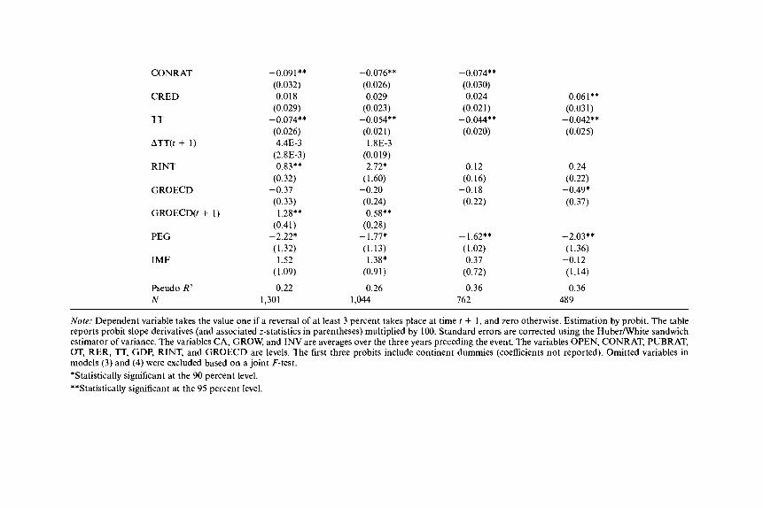
Fig. 8.1 Note: Data for 100 reversals from 105 countries, 1970-96. A reversal is defined as an average improvement in the current account (net of official transfers) of at least 3 percent over a period of three years with respect to the previous three years. “Turbulent” periods are those within three years of a current account reversal, and “tranquil” periods are those that are not within three years of a reversal. For each variable, the plots depict the difference between the variable mean during turbulent periods and its mean during periods of tranquility, as well as the 2-standard-deviation band. The upper left-hand panel depicts instead the differ- ence between the medians during the two periods. Scales and data vary by panel.
Current account reversals: whole sample
al. (1995). The basic idea of this event-study methodology is to distinguish between periods of “turbulence”-here those within three years of a re- versal event-and the remaining, “tranquil” periods. Graphs allow a com- parison of variables during turbulent periods with their (average) values during tranquil periods.
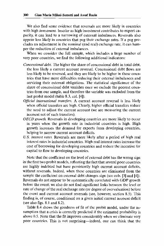
Figures 8.1 and 8.2 depict the behavior of a set of variables during peri- ods of turbulence (around the time of reversals) for the whole sample and for the reduced sample comprising thirty-nine middle-income countries, respectively. Each panel shows deviations of these variables from their means during periods of tranquility, except for the upper left-hand panel,
Current Account Reversals and Currency Crises 295
15
10
5
0
1
0
-1
-2 -3
5
0
-5
1
.5
0
-.5
Nominal Depreciation
1 I 7
-3 3
Resewesllmports
-3 3
Consumption Growth
-3 3
Official Transfers
-1 '"RV? 0 i+*- -20 -10
-3 3 -3 3
Real Exchange Rate Current Account
0 5p*e -;p+: -5
-3 3 -3 3
Investment Rate Growth
lo, w; -1 0
-3 3
Fiscal Balance Terms of Trade
.ikw; -.5 -1
-3 3 -3 3
Foreign Direct Investment Interest PaymenWGDP
Fig. 8.2 Note: Data for 47 reversals from 39 countries, 1970-96. See fig. 8.1 note.
Current account reversals: middle-income sample
which plots the median rate of depreciation in turbulent periods, as a devi- ation from the sample median in tranquil periods. The plotted values for the remaining panels refer to reversal events and are the means (plus or minus 2 standard deviations) of the variable during each year of the rever- sal episode (from t - 3 to t + 3 ) as a deviation from the sample mean of the variable during tranquil periods. Hence a positive value for a variable indicates that it tends to be higher in turbulent than in tranquil periods.6
The figures show that the real exchange rate starts out more appreciated than average before reversal periods and then depreciates throughout the
6. One potential problem with this methodology is that the time distribution of reversal episodes is concentrated in the 1980s, and therefore the characteristics of the reversal events we identify are in part influenced by the characteristics of the 1980s with respect to the 1970s and the 1990s. However, the graphs restricted to the 1980s show the same overall pattern as fig. 8.1.

296 Gian Maria Milesi-Ferretti and Assaf Razin
period. This comovement between the real exchange rate and the current account is clearly in line with the standard analysis of the transfer prob- lem. The panel depicting the behavior of the nominal exchange rate shows indeed an acceleration in the median rate of currency depreciation that occurs a couple of years before reversals. Reversals tend also to be pre- ceded by unfavorable terms of trade, low foreign exchange reserves, a high interest burden of external debt, low consumption growth, and a high but declining fiscal deficit. After a reversal occurs, reserves tend to rise, and the fiscal balance continues to improve, and the real exchange rate to de- preciate. Note also that no clear pattern for output growth characterizes the period preceding or following a reversal. This finding runs counter to the conventional wisdom that sharp reductions in current account deficits reflect an external crisis and that they are achieved by protracted domestic output compression so as to reduce import demand.
We then use multivariate probit analysis to examine whether a set of explanatory variables helps to predict whether a country is going to experi- ence a reversal in current account imbalances. More specifically, we esti- mate the probability of a reversal occurring at time t (meaning a 3 percent average decline in the current account deficit between t and t + 2 with respect to the period between t - 1 and t - 3 ) as a function of variables at t - 1 and of contemporaneous exogenous variables (terms of trade, industrial country growth, and world interest rates). The choice of the set of explanatory variables is motivated by existing research on currency and banking crises, as well as by our previous work comparing episodes of persistent current account deficits, which identified a number of potential indicators of sustainability. Among them we include the current account deficit (CA), economic growth (GROW), investment rate (INV), GDP per capita (GDP), real effective exchange rate (RER), openness to trade (OPEN), foreign exchange reserves as a fraction of imports (RES), exter- nal official transfers as a fraction of GDP (OT), ratio of external debt to GDP (DEBTY), share of concessional debt in total debt (CONRAT), share of public debt in total debt (PUBRAT), and ratio of credit to GDP (CRED-a proxy for financial development). Other variables, such as the ratio of FDI flows to GDP (FDI) and the share of short-term debt in total debt (SHORT) were excluded from the probit because they turned out to be economically and statistically insignificant. We excluded the fiscal deficit because of problems with data availability-it did not enter sig- nificantly in the probit analysis, and it reduced sample size considerably. Note that the definition of the event is based on changes in the current account balance, and we therefore believe it is important to control for the level of the current account balance prior to the reversal.
Among the “exogenous” variables we include the lagged and contemp- oraneous real interest rate in the United States (RINT-as a proxy for world interest rates), lagged and contemporaneous rate of growth in
Current Account Reversals and Currency Crises 297
OECD countries (GROECD), lagged level of the terms of trade (TT), and change in the terms of trade in the reversal period (ATT(t + 1)). We also use the dummy for the exchange rate regime (PEG) and the dummy for an IMF program (IMF).’ For some of the lagged explanatory variables, namely, the current account, the rate of growth, and the investment share, we use a three-year average (over the period t - 1 to t - 3 ) rather than their level at t - 1, to ensure consistency in the way we measure reversals.
It is clearly incorrect to interpret this probit analysis in a “structural” way, given that many of the explanatory variables are endogenous. Never- theless, the analysis can provide a useful multivariate statistical character- ization of reversal events as well as identify potential “leading indicators.” Probit results are presented in table 8.3.
Overall, the empirical analysis identifies a number of robust predictors of reversals in current account imbalances, regardless of the sample defi- nition:
Current account deficit. Not surprisingly, reversals are more likely in coun- tries with large current account deficits. This result is consistent with solvency and willingness-to-lend considerations.
Foreign exchange reserves. Countries with lower reserves (expressed in months of imports) are more likely to experience reversals. Clearly, low reserves make it difficult to sustain large external deficits and may re- duce the willingness to lend of foreign investors. The ratio of reserves to M2, indicated by Calvo (1997) and others as a key predictor of bal- ance-of-payments crises, also appears to signal reversals ahead of time in our sample.
GDPper capita. Countries with higher GDP per capita are more likely to experience reversals. The coefficient on this variable captures the diffi- culty extremely poor countries have reversing external imbalances. The positive coefficient is also consistent with the theory of stages in the balance of payments: as a country gets richer, a reduction in deficits (or a shift to surpluses) is more likely.
Terms of trade. Reversals seem more likely in countries with worsened terms of trade. One interpretation of this finding is that countries that have suffered terms-of-trade deterioration are more likely to experience reversals of capital flows and may therefore be forced to adjust. The evidence is also in line with what is suggested by Kraay and Ventura (2000), since the countries in our sample are almost entirely net debtors, and by Tornell and Lane (1998), who argue that the “common pool problem” may be exacerbated by favorable terms-of-trade shocks, thus leading to a more than proportional increase in absorption.
7. Santaella (1996) and Knight and Santaella (1997) study the determinants of IMF pro- grams and characterize the stylized facts that precede them.
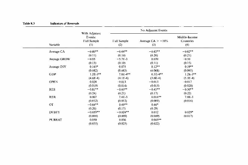
Table 8.3 Indicators of Reversals
No Adjacent Events With Adjacent
Events: Middle-Income Full Sample Full Sample Average CA > - 10% Countries
Variable (1) (2) (3) (4)
Average CA
Average GROW
Average INV
GDP
OPEN
RES
RER
OT
DEBTY
PUBRAT
-0.60** (0.1 I )
-0.05 (0.13) 0.145*
(0.082) 1.2E-3**
(4.6E-4) -0.028 (0.019)
-0.81** (0.24) 0.007
(0.0 12) -0.64** (0.20)
(0.009) 0.050
(0.035)
-0.019**
-0.44** (0.10)
-5.7E-3 (0.10) 0.075
(0.063) 7.8E-4**
(4.1 E-4) -0.013 (0.014)
-0.60** (0.21) 7.4E-3
(0.012) -0.49** (0.17)
(0.009) 0.036
(0.025)
-0.024**
-0.63** (0.20) 0.070
(0.1 1) 0.12**
(0.068) 6.5E-4* *
(3.6E-4)
(0.015) -0.45** (0.17) 0.016**
(0.009) -0.44* (0.29) 0.012
(0.009) 0.045**
(0.022)
-0.013
-0.62** (0.21)
-0.10 (0.15) 0.19**
(0.095) 1.2E-3**
(5.3E-4) -0.017 (0.020)
-0.50** (0.22) 7.OE-3
(0.016)
0.029* (0.017)
CONRAT
CRED
TT
ATT(t + 1)
RINT
GROECD
GROECD(f + 1)
PEG
IMF
Pseudo R2 N
-0.091** (0.032) 0.018
(0.029) -0.074** (0.026) 4.4E-3
0.83** (0.32)
(0.33)
(0.41) -2.22* (1.32) 1.52
(1.09)
0.22
(2.8E-3)
-0.37
1.28**
1,301
-0.076** (0.026) 0.029
(0.023) -0.054** (0.021) 1.8E-3
(0.019) 2.72*
(1.60) -0.20 (0.24) 0.58**
(0.28) - 1.77* (1.13) 1.38*
(0.91)
0.26 1,044
-0.074** (0.030) 0.024
(0.021) -0.044** (0.020)
0.12 (0.16)
-0.18 (0.22)
- 1.62** (1.02) 0.37
(0.72)
0.36 162
0.061** (0.03 1)
-0.042** (0.025)
0.24
-0.49* (0.22)
(0.37)
-2.03** (1.36)
-0.12 (1.14)
0.36 489
Note: Dependent variable takes the value one if a reversal of at least 3 percent takes place at time t + 1, and zero otherwise. Estimation by probit. The table reports probit slope derivatives (and associated z-statistics in parentheses) multiplied by 100. Standard errors are corrected using the HuberlWhite sandwich estimator of variance. The variables CA, GROW, and INV are averages over the three years preceding the event. The variables OPEN, CONRAT, PUBRAT, OT, RER, TT, GDP, RINT, and GROECD are levels. The first three probits include continent dummies (coefficients not reported). Omitted variables in models (3) and (4) were excluded based on a joint F-test. *Statistically significant at the 90 percent level. **Statistically significant at the 95 percent level.
300 Gian Maria Milesi-Ferretti and Assaf Razin
We also find some evidence that reversals are more likely in countries with high investment. Insofar as high investment contributes to export ca- pacity, it can lead to a narrowing of external imbalances. Reversals also appear less likely in countries that peg their exchange rates. If a peg pre- cludes an adjustment in the nominal (and real) exchange rate, it can ham- per the reduction of external imbalances.
When we consider the full sample, which includes a large number of very poor countries, we find the following additional indicators:
Concessional debt. The higher the share of concessional debt in total debt, the less likely a current account reversal. Concessional debt flows are less likely to be reversed, and they are likely to be higher in those coun- tries that have more difficulties reducing their external imbalances and servicing their external obligations. The statistical significance of the share of concessional debt vanishes once we exclude the poorest coun- tries from our sample, and therefore the variable was excluded from the last probit model (table 8.3, col. [4]).
Oficial international transfers. A current account reversal is less likely when official transfers are high. Clearly, higher official transfers reduce the need to adjust the current account (we are measuring the current account net of such transfers).
OECD growth. Reversals in developing countries are more likely to occur in years when the growth rate in industrial countries is high. High growth increases the demand for exports from developing countries, helping to narrow current account deficits.
U S . interest rates. Reversals are more likely after a period of high real interest rates in industrial countries. High real interest rates increase the cost of borrowing for developing countries and reduce the incentive for capital to flow to developing countries.
Note that the coefficient on the level of external debt has the wrong sign in the first two probit models, reflecting the fact that several poor countries are highly indebted but have persistently high current account deficits, without reversals. Indeed, when these countries are eliminated from the sample the coefficient on external debt changes sign (see cols. [3] and [4]). Reversals do not appear to be systematically correlated with GDP growth before the event; we also do not find significant links between the level or rate of change of the real exchange rate (or degree of overvaluation) before the event and current account reversals (see, however, section 8.5). This finding is, of course, conditional on a given initial current account deficit (see also figs. 8.1 and 8.2).
Table 8.4 shows the goodness of fit of the probit model, under the as- sumption that a crisis is correctly predicted if the estimated probability is above 0.5. Note that the fit improves considerably when we eliminate very poor countries. This is not surprising-indeed, one can think that the

Current Account Reversals and Currency Crises 301
Table 8.4 Goodness of Fit: Reversal Models
Predicted
Actual 0 1 Total
0 1 Total
0 1 Total
0 1 Total
0 1 Total
Model (1) 1,186 7 1,193
101 7 108 1,287 14 1,301
Model (2) 972 4 976 60 8 68
1,032 12 1,044 Model (3)
695 6 70 1 44 17 61
739 23 762
444 4 448 28 13 41
412 17 489
Model (4)
determinants of swings in the current account can differ substantially be- tween countries that rely exclusively on official transfers, mostly on con- cessional terms, and those that have more access to international capital markets.
The results presented so far have to be interpreted taking into account the fact that the empirical analysis aggregates reversal events that have quite different features; it includes such full-fledged balance-of-payments crises as, say, Mexico 1982 and improvements in the current account spurred by favorable terms-of-trade developments or timely corrections in macroeconomic policy. A better understanding of the dynamics of current account reversals and of the role of economic policy will require a classifi- cation of these events based on their salient features (terms-of-trade shocks, swings in capital flows, etc.). This would provide an opportunity for a closer match between intertemporal models of current account deter- mination and developing country data.
8.5 Current Account Reversals and Output Performance
This section examines the behavior of output growth in countries that experienced sharp reductions in current account imbalances. We focus on two issues: first, whether reversals are costly in terms of output and, sec- ond, what factors determine a country’s rate of growth during a reversal period. Output costs clearly arise when reversals are associated with mac- roeconomic crises and more generally can be due to macroeconomic ad-
302 Gian Maria Milesi-Ferretti and Assaf Razin
justment and sectoral reallocation of resources. For the purpose of this “before and after” analysis we selected the 3 percent event definition and we eliminated adjacent events.8 This identifies 100 reversal episodes for the definition excluding official transfers.
The first interesting finding is that the median change in output growth between the period after and that before the event is around zero, sug- gesting that reversals in current account deficits are not necessarily associ- ated with domestic output compression. However, output performance is very heterogeneous. For example, Uruguay’s average growth was - 7 per- cent in the period 1982-84, compared to 4 percent in the period 1979-81; Malaysia went instead from growth of 2.4 percent in 1984-86 to growth of close to 8 percent over the following three years.
Our dependent variable in the regression analysis is the average rate of output growth during the three years of the reversal period, as a deviation from the OECD average during the same period. We take the deviation of growth from the OECD average because reversal events occur in differ- ent years, and we want to (roughly) correct each country’s performance for the overall behavior of the world economy during that period. Our explanatory variables include average growth (also as a deviation from the OECD average), average investment, average current account balance, GDP per capita (a “conditional convergence” term), ratio of external debt to GDP (DEBTY), overvaluation of the real exchange rate, official trans- fers, and U.S. real interest rates. They are all dated prior to the rever~a l .~ Results are presented in table 8.5.
The table shows that countries more open to trade and with less ap- preciated levels of the exchange rate before the event are likely to grow faster after the event. The size of the point estimates indicates that the effects of these variables are also economically significant: for example, a country that has an overvaluation of 10 percent before the reversal is likely to grow 0.7 percent slower for the following three years. We also find some evidence that countries with high external debt and those that receive high official transfers tend to grow more slowly. The latter finding could of course simply reflect the fact that poor countries that grow slowly tend to receive large transfers. Indeed, when we exclude countries with low per capita income, the coefficient on official transfers changes sign and be- comes statistically insignificant (regression not reported). Note also that the correlation between growth before and after the event is low and statis- tically insignificant, with the exception of the regression for the group of middle-income countries.
Overall, the empirical analysis seems to provide a reasonable character-
8. In Milesi-Ferretti and Razin (1998) we grouped events occurring in adjacent years for the same country, counting them as a single, longer lasting reversal.
9. All averages are calculated over the three-year period preceding the reversal. The per- centage change in the terms of trade between the two periods was statistically insignificant and was excluded from the regression so as to increase sample size.

Current Account Reversals and Currency Crises 303 ~
Table 8.5 Consequences of Reversals
Regional Dummies
Average CA Middle-Income Variable Full Sample Full Sample > -10% Countries
Lagged dependent 0.10 0.10 0.10 0.32** variable (0.1 1) (0.1 1) (0.10) (0.12)
CA -0.10 -0.14* -0.13 -0.07 (0.08) (0.07) (0.08) (0.09)
(0.017) (0.016) (0.018) (0.023) OPEN 0.030** 0.021* 0.026** 0.031 *
(0.01 1) (0.01 1) (0.013) (0.016)
(0.07) (0.079) (0.01 1) (0.009)
(0.17) (0.16) (0.17) (0.18)
(0.11) (0.10) (0.35)
(2.4E-4) (2.6E-4) -2.9E-4 ( - 2.8E-4)
OVERVA -0.076** -0.078** -0.069** -0.070**
DEBTY -0.018** -0.016** -0.018 -0.025**
RINT -0.23 -0.29* -0.20 -0.42
OT -0.29** -0.31** -0.55
GDP -3. I E-4 - 1.4E-4 -3.OE-4 - 1.6E-4
INV 0.058 0.067 -0.067 -0.037 (0,044) (0.048) (0.044) (0.067)
R2 0.35 0.40 0.44 0.58 N 84 84 66 44
Note: Dependent variable is output growth during reversal period, a three-year average, expressed as deviation from the OECD average during the same period. Estimation by OLS with White’s correction for heteroskedasticity. Numbers in parentheses are standard errors. The explanatory variables CA and INV are averages over the three years preceding the event; the variables OPEN, GDP, RER, TT, OT, and DEBTY are levels the year before the event. *Statistically significant at the 90 percent level. **Statistically significant at the 95 percent level.
ization of short- or medium-run output performance during periods of substantial reduction in external imbalances. A noteworthy finding is that reversal events seem to entail substantial changes in macroeconomic per- formance between the period before and the period after the crisis but are not systematically associated with a growth slowdown.
8.6 Predictors of Currency Crashes
In this section we extend and refine work by Frankel and Rose (1996), by considering a longer sample and alternative definitions of currency cri- ses. We use four definitions of currency crises; the first (CRISISl), used by Frankel and Rose (1 996), requires an exchange rate depreciation vis-a- vis the dollar of 25 percent, which is at least 10 percent higher than the depreciation the previous year. The main problem with this definition is that it considers as a crisis an episode in which the rate of depreciation

304 Gian Maria Milesi-Ferretti and Assaf Razin
increases from, say, 50 to 61 percent. To avoid capturing the large ex- change rate fluctuations associated with high-inflation episodes, the sec- ond definition (CRISIS2) requires, in addition to a 25 percent deprecia- tion, at least a doubling in the rate of depreciation with respect to the previous year and a rate of depreciation the previous year below 40 per- cent. The third and fourth definitions (CRISIS3 and CRISIS4) focus on those episodes in which the exchange rate was relatively stable the previous year and that therefore may be closer to the concept of currency crisis implicit in theoretical models. CRISIS3 requires a 15 percent minimum rate of depreciation, a minimum 10 percent increase in the rate of depre- ciation with respect to the previous year, and a rate of depreciation the previous year of below 10 percent. Finally, CRISIS4 is analogous to CRISIS3 with the additional requirement that the exchange rate be pegged the year before the crisis.
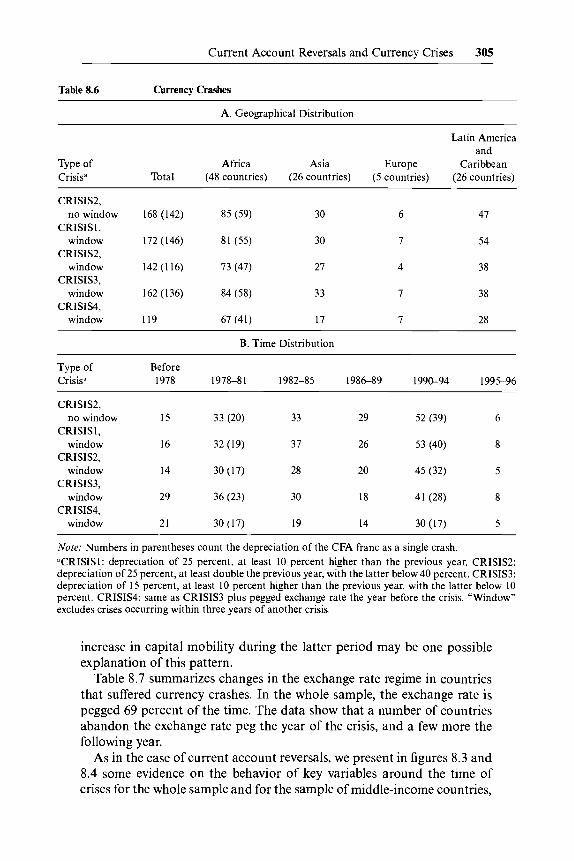
We do not consider as a crisis any event that occurs within three years of another crisis; we therefore construct a “window” around each crisis event that is distinguished from periods of tranquility. This reduces the total number of crises; table 8.6 summarizes the currency crisis episodes according to the different definitions.
There is clearly a large degree of overlap between these definitions of crises. Practically all episodes in CRISIS2 (1 38 of them) are also episodes of CRISIS1.I0 The overlap between CRISIS3 and CRISIS1 (or CRISIS2) is smaller (109 cases) but still significant. Note also that the number of “crashes” depends crucially on whether one counts countries that experi- enced a crash or currencies that crashed. The six members of the Central African Economic and Monetary Union (Cameroon, Central African Re- public, Chad, Congo, Equatorial Guinea, and Gabon), the seven members of the West African Economic and Monetary Union (Benin, Burkina Faso, Cbte d’Ivoire, Mali, Niger, Senegal, and Togo) plus the republic of the Comoros share the same currency (the CFA franc), which was set at a fixed rate vis-a-vis the French franc until 1994 and then devalued by 50 percent.” Our definition of crisis therefore captures fourteen country epi- sodes that year, and also in 1981 (because of the depreciation of the French franc vis-a-vis the dollar).
The geographical distribution of currency crashes shows that African and Latin American countries tend to experience more crashes than Asian countries (adjusting by the number of countries in the sample). Recall, however, that the recent Asian currency crashes are not in the sample. The time distribution of currency crashes is more uniform than the distribution of reversals, with the highest number of crashes in the early 1980s (the period of the debt crisis) and, more surprisingly, in the early 1990s. The
10. The effects of windowing account for the CRISIS2 episodes that are not also CRISIS1. 11. Technically, the Islamic Federal Republic of Comoros uses a different currency, the
CV, which is tied to the French franc in an analogous fashion to the CFA.
Current Account Reversals and Currency Crises 305
Table 8.6 Currency Crashes
A. Geographical Distribution
Latin America and
Type of Africa Asia Europe Caribbean Crisis” Total (48 countries) (26 countries) (5 countries) (26 countries)
CRISIS 2,
CRISIS1,
CRISIS2,
CRISIS3,
CRISIS4,
no window 168 (142) 85 (59) 30 6 47
window 172 (146) 81 (55) 30 7 54
window I42 (116) 73 (47) 27 4 38
window 162 (136) 84 (58) 33 7 38
window 119 67 (41) 17 7 28
B. Time Distribution
Type of Before Crisis’ 1978 1978-81 1982-85 198689 1990-94 1995-96
CRISIS2,
CRISIS1,
CRISIS2,
CRISIS3,
CRISIS4,
no window 15 33 (20) 33 29 52 (39) 6
window 16 32 (19) 37 26 53 (40) 8
window 14 30 (17) 28 20 45 (32) 5
window 29 36 (23) 30 18 41 (28) 8
window 21 30 (17) 19 14 30 (17) 5
Note: Numbers in parentheses count the depreciation of the CFA franc as a single crash. “CRISIS1: depreciation of 25 percent, at least 10 percent higher than the previous year. CRISIS2: depreciation of 25 percent, at least double the previous year, with the latter below 40 percent. CRISIS3: depreciation of 15 percent, at least 10 percent higher than the previous year, with the latter below 10 percent. CRISIS4: same as CRISIS3 plus pegged exchange rate the year before the crisis. “Window” excludes crises occurring within three years of another crisis.
increase in capital mobility during the latter period may be one possible explanation of this pattern.
Table 8.7 summarizes changes in the exchange rate regime in countries that suffered currency crashes. In the whole sample, the exchange rate is pegged 69 percent of the time. The data show that a number of countries abandon the exchange rate peg the year of the crisis, and a few more the following year.
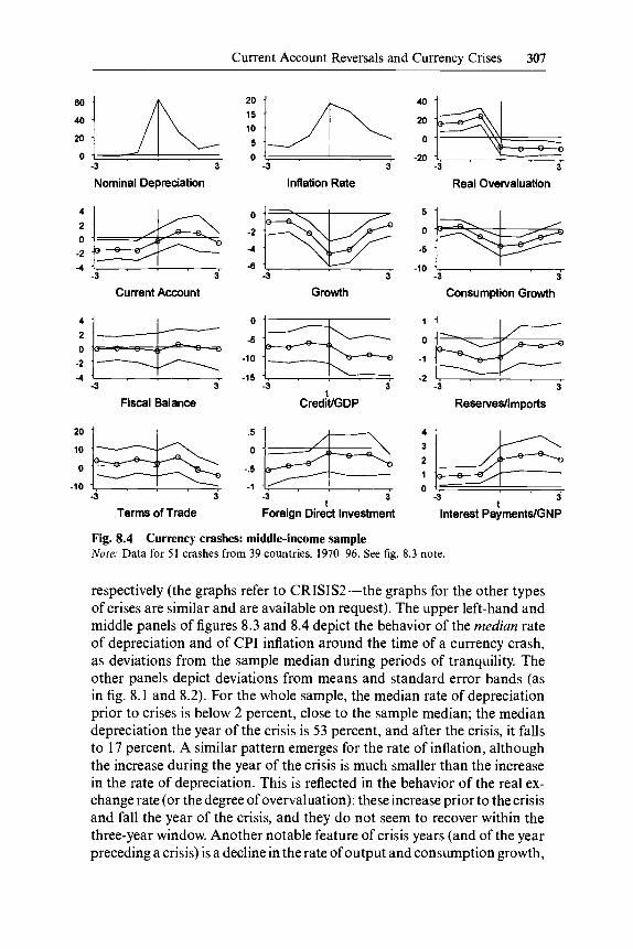
As in the case of current account reversals, we present in figures 8.3 and 8.4 some evidence on the behavior of key variables around the time of crises for the whole sample and for the sample of middle-income countries,

00
40
20
0
2
0
-2
-4
2
0
-2
-4
5
0
-5
-10
Table 8.7 Currency Crashes and Exchange Rate Regime
Peg Year Peg Year Peg Year Type of Crisis Totala before Crisis of Crisis after Crisis
CRISIS1, window I64 99 87 79 CRISIS2, window 136 97 83 76 CRISIS3, window 146 1 I4 98 89 CRISIS4, window 115 115 95 87
=Total number of crises for which data on exchange rate regime before and after crisis are available.
Nominal Depreciation
-3 3
Current Account
,
-3 3
Fiscal Balance
& -3 3
Terms of Trade
! I>, 5 0
-3 3
Inflation Rate
I -3 3
Growth
-1 -5 0 3 E 3
CreditlGDP
-.5
-1 .: -3 & 3
Foreign Dirict Investment
-40 i I
-3 3
Real Overvaluation
-3 3
Consumption Growth
-1
-1.5 -,: -3 E 3
Reservesllmports
1
0 -3 3
t Interest PaymentdGNP
Fig. 8.3 Currency crashes: whole sample Note: Data for 142 crashes from 105 countries, 1970-96. A crash is defined as a nominal exchange rate depreciation of at least 25 percent, which is at least double the previous year’s depreciation rate, as long as the latter is below 40 percent. “Turbulent” periods are those within three years of a currency crash, and “tranquil” periods are those that are not within three years of a crash. For each variable, the plots depict the difference between the variable mean during turbulent periods and its mean during periods of tranquility, as well as the 2- standard-deviation band. The upper left-hand and middle panels depict instead the differ- ence between the medians during the two periods. Scales and data vary by panel.
Current Account Reversals and Currency Crises 307
20 :: 0 -3 k 3
Nominal Depreciation
40
0 5 - 0 r -20
-3 3
Inflation Rate
Growth
I r
-3 3
Current Account
4
2 0
-2
4 3 3
Fiscal Balance
-1-:
-15 -3 3
1 CrediVGDP
1
0
-1
-2
0
-1 :: 0 -3 b 3
Terms of Trade
4
3
2 1 -.5
-1 .: -3 e 1 3 0
Foreign Direct Investment
-3 k 3
Real Overvaluation
I
-3 3
Consumption Growth
-3 ' 3
Resewedmports
-3 3 t
Interest PaymentsfGNP
Fig. 8.4 Currency crashes: middle-income sample Note: Data for 51 crashes from 39 countries, 1970-96. See fig. 8.3 note.
respectively (the graphs refer to CRISIS2-the graphs for the other types of crises are similar and are available on request). The upper left-hand and middle panels of figures 8.3 and 8.4 depict the behavior of the median rate of depreciation and of CPI inflation around the time of a currency crash, as deviations from the sample median during periods of tranquility. The other panels depict deviations from means and standard error bands (as in fig. 8.1 and 8.2). For the whole sample, the median rate of depreciation prior to crises is below 2 percent, close to the sample median; the median depreciation the year of the crisis is 53 percent, and after the crisis, it falls to 17 percent. A similar pattern emerges for the rate of inflation, although the increase during the year of the crisis is much smaller than the increase in the rate of depreciation. This is reflected in the behavior of the real ex- change rate (or the degree of overvaluation): these increase prior to the crisis and fall the year of the crisis, and they do not seem to recover within the three-year window. Another notable feature of crisis years (and of the year preceding a crisis) is a decline in the rate of output and consumption growth,

308 Gian Maria Milesi-Ferretti and Assaf Razin
with a rebound taking place after the crisis. The median consumption growth rate over the three years preceding a crisis is 3.3 percent, the year of the crisis, 0.2 percent, and the following three years, 2.2 percent. For out- put growth, we get 2.6, 1.4, and 3.1 percent, respectively. Not surprisingly, foreign exchange reserves around crisis periods tend to be lower than dur- ing tranquil periods and the terms of trade less favorable. There is some evidence that current account deficits are larger before crises than in tran- quil periods; however, the figures show an improvement in the current account position after the devaluation only for middle-income countries.
We turn now to multivariate probit analysis. We estimate the probability of a currency crisis at time t + 1 as a function of a set of explanatory var- iables at time t and of external factors at time t and t + 1. The set of ex- planatory variables is similar to the set we used for reversals; here we also report results using the ratio of reserves to M2 (RESM2) as an alternative to reserves measured in months of imports (RES). Results are presented in table 8.8. Columns (1) through (4) report probit analysis using the full sample and the four different definitions of crises, while columns (5) and (6) report the results for the sample of thirty-nine middle-income coun- tries. Overall, these results suggest some robust leading indicators of cur- rency crashes, regardless of the precise definition of crash:
Foreign exchange reserves. Crashes are more likely in countries with low foreign exchange reserves, measured as a fraction of imports or as a fraction of M2.I2 This finding is clearly in line with theoretical models of currency crises.
Real exchange rate overvaluation. Crashes are more likely in countries in which the real exchange rate is appreciated relative to its historical aver- age. This finding suggest that even the crude measure of exchange rate misalignments adopted here provides some useful information on the likelihood of exchange rate collapse.I3
U S . interest rates. Crashes are more likely when real interest rates in the United States are (or have been) high. Higher interest rates in industrial countries make investment in developing countries less attractive and are more likely to cause reversals in capital flows.
Growth in industrial countries. Crashes are more likely if growth in indus- trial countries has been sluggish. A possible channel is through lower demand for developing country exports, a decline in foreign exchange reserves, and a more likely collapse of the currency.
Terms oftrade. A crisis is less likely when the terms of trade are favorable.
12. The regressions using RESM2 instead of RES are not reported but are available from the authors. Klein and Marion (1997) report similar results using the ratio of reserves to MI for a sample of Latin American countries.
13. A potential problem with this finding is that the definition of the benchmark as the sample average implies a tendency for mean reversion.
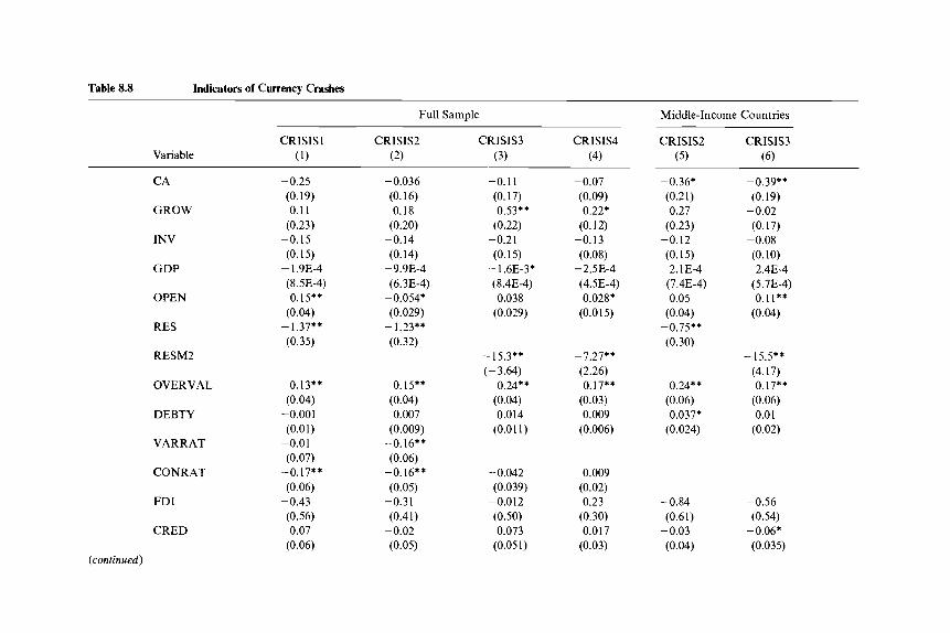
Table 8.8 Indicators of Currency Crashes
Full Sample Middle-Income Countries
CRISIS1 CRISIS2 CRISIS3 CRISIS4 CRISIS2 Variable (1) (2) (3) (4) (5)
CA
GROW
INV
GDP
OPEN
RES
RESM2
OVERVAL
DEBTY
VARRAT
CONRAT
FDI
CRED
(continued)
-0.25 (0.19) 0.11
(0.23) -0.15 (0.15)
(8.5E-4)
(0.04)
(0.35)
- 1.9E-4
-0.15**
- 1.37**
0.13** (0.04)
-0,001 (0.01)
-0.01 (0.07)
-0.17** (0.06)
(0.56) 0.07
(0.06)
-0.43
-0.036 (0.16) 0.18
(0.20) -0.14 (0.14) - 9.9E-4 (6.3E-4)
-0.054* (0.029)
(0.32) - 1.23**
0.15** (0.04) 0.007
(0.009)
(0.06)
(0.05) -0.31 (0.41)
-0.02 (0.05)
-0.16**
-0.16**
-0.11 (0.17) 0.53**
(0.22) -0.21
- 1.6E-3* (8.4E-4) 0.038
(0.029)
(0.15)
-15.3** (-3.64)
0.24** (0.04) 0.014
(0.01 1)
-0.042 (0.039)
-0.012 (0.50) 0.073
(0.051)
-0.07 (0.09) 0.22*
(0.12) -0.13 (0.08)
-2.58-4 (4.5E-4) 0.028*
(0,015)
-7.27** (2.26) 0.17**
(0.03) 0.009
(0.006)
0.009 (0.02) 0.23
(0.30) 0.017
(0.03)
-0.36* (0.21) 0.27
(0.23) -0.12 (0.15) 2.1 E-4
(7.4E-4) 0.05
(0.04)
(0.30) -0.75**
0.24** (0.06) 0.037*
(0.024)
-0.84 (0.61)
(0.04) -0.03
CRISIS3 (6)
-0.39** (0.19)
-0.02 (0.17)
-0.08 (0.10) 2.4E-4
(5.78-4) 0.11**
(0.04)
- l5.5** (4.17) 0.17**
(0.06) 0.01
(0.02)
-0.56 (0.54)
(0.035) -0.06*
Table 8.8 (continued)
Full Sample Middle-Income Countries
CRISIS1 CRISIS2 CRISIS3 CRISIS4 CRISIS2 CRISIS3 Variable (1) (2) ( 3 ) (4) ( 5 ) (6)
TT
ATT(t + 1)
RINT
RINT(t + 1)
GROECD
GROECD(t + 1)
PEG
IMF
Pseudo R2 N
-0.11** (0.04)
-0.10* (0.06) 0.34
(0.55) 1.24**
(0.51) - l.74** (0.54)
-0.20 (0.66)
-7.57** (2.51)
-2.84** (1.45)
0.29 838
-0.10** (0.04)
-0.08 (0.05)
-0.20 (0.48)
(0.44)
(0.48)
(0.57)
(1.78)
(1.30)
0.24
1.08**
-1.34**
-0.24
-2.61
-2.58*
897
-0.061 (0.038)
-0.099* (0.053)
-0.014 (0.50)
(0.46)
(0.50) -0.53 (0.62) 1.34
(1.59) 0.63
(1.64)
0.27
1.36**
-1.61**
878
-0.060** (0.023)
-0.066** (0.031)
(0.29) 0.62**
(0.28)
(0.28) 0.13
(0.35)
-0.31
-0.49**
0.58 (0.99)
0.29 985
-0.064* (0.037)
1.15** (0.37)
-0.49 (0.48)
(0.58)
(1.43)
1.32**
-0.60
-2.32 (- 1.38)
0.36 474
-0.057** (0.030)
0.45* (0.27)
-0.84** (0.42) 0.37
(0.43) 2.26*
(1.38) 1.01
(1.44)
0.36 472
Note: Dependent variable takes the value one if a currency crash occurs at time t + 1, and zero otherwise. Estimation by probit. The table reports probit slope derivatives (and associated z-statistics in parentheses) multiplied by 100. The variables CA, GROW, and INV are averages over the three years preceding the event. Variables are dated at time t unless otherwise marked. Regressions include continent dummies (coefficients not reported). Omitted variables in models ( 5 ) and (6) were excluded based on a joint F-test. *Statistically significant at the 90 percent level. **Statistically significant at the 95 percent level.
Current Account Reversals and Currency Crises 31 1
This is another intuitive finding: better terms of trade should improve a country’s creditworthiness (and its cash flow) and make it less vulner- able to speculative attacks.
When we use the whole sample, a number of other factors are good leading predictors of crisis according to CRISIS1 and CRISIS2, but not CRISIS3 and CRISIS4:
Share of concessional debt. Crashes are less likely in countries with large shares of debt on concessional terms. This may be explained by the fact that these flows are less likely to be reversed.
Openness. More open economies are less likely to suffer exchange rate crashes. This evidence suggests that when we include crises associated with high-inflation episodes the benefits of trade openness outweigh the higher vulnerability to external shocks. This is not the case, however, when we focus on crashes that were preceded by more stable exchange rates (see cols. [3], [4], and [6]).14
IMFdummy. Countries with IMF programs in place are less likely to suffer crashes the following year. In addition to a possible “credibility effect,” this finding could reflect the fact that programs are approved or remain in place in countries willing to strengthen their fundamentals.
For the sample of middle-income countries we also find that a crash is more likely when the current account deficit is large. For the full sample, which includes several low-income countries with very large current ac- count deficits throughout the period, the current account has the expected sign but is statistically insignificant. The finding that countries with pegged exchange rates are less likely to suffer crashes of type 1 may simply reflect the fact that the rate of depreciation tends to be lower in countries with pegged exchange rates than in countries with floating exchange rates (the median rate of depreciation in the sample for countries that peg is zero, while it is 12 percent for countries with floating exchange rates). In- deed, when we limit the definition of crisis to countries with low initial rates of depreciation (CRISIS3 or CRISIS4) the coefficient on the peg variable changes sign.
Table 8.9 reports the goodness of fit of the model. As in the case of reversals, goodness of fit improves when the sample is restricted to middle- income countries. Note also the difference in the classification accuracy for the full sample between CRISIS1 and CRISIS2: this is due to the fact that the model predicts easily accelerations in the rate of depreciation as- sociated with episodes of high inflation. Overall, these results are broadly in line with those reported by Frankel and Rose (1996). They highlight domestic factors, such as the degree of overvaluation and the level of re-
14. Klein and Marion (1997) find that openness significantly reduces the likelihood of a devaluation in a sample of Latin American countries that peg their exchange rate.

312 Gian Maria Milesi-Ferretti and Assaf Razin
Table 8.9 Goodness of Fit: Currency Crash Models
Predicted
Actual 0 1 Total
0 1 Total
0 1 Total
0 1 Total
0 1 Total
0 1 Total
0 1 Total
Model (1) 725 9
71 33 796 42
808 5 70 14
878 19
779 7 69 23
848 30
913 4 56 12
969 16
430 3 26 15
456 18
422 4 30 16
452 20
Model (2)
Model (3)
Model (4)
Model ( 5 )
Model (6)
734 104 838
813 84
897
786 92
878
917 68
985
433 41
474
426 46
472
serves, and external factors, such as growth and interest rates in industrial countries and the terms of trade, that tend to precede currency crashes.
8.7 Currency Crises and Output Performance
In this section we characterize output performance after a currency cri- sis. The objective is twofold: first, to identify stylized facts regarding the behavior of macroeconomic variables before and after crises and, second, to investigate which factors help to explain output growth after crises.
A stylized fact that emerged from the analysis of the previous section is that output and consumption growth the year of the crisis are lower than the averages during the three preceding years and during the three follow- ing years. This finding suggests that we are indeed picking up events that have disruptive effects on macroeconomic activity, at least in the short run. One telling example is Korea, which experienced a currency crisis (according to the first three definitions) in 1980. Its average growth in the three years preceding the crisis was above 10 percent; in 1980 output fell by close to 3 percent, and in the three successive years growth was back
Current Account Reversals and Currency Crises 313
at 8 percent. In the regression analysis we explore the determinants of output performance in the three years following a currency crash. Our dependent variable is the average growth rate in the three years following the crash, as a deviation from the OECD average during the same period. Our independent variables include the average growth rate in the three years preceding the crisis and growth rate the year of the crisis (both ex- pressed as deviations from the OECD average during those periods), aver- age investment rate and current account balance the three years prior to the crisis, change in the terms of trade between the two periods, as well as ratio of debt to GDP, degree of real exchange rate overvaluation, GDP per capita, real interest rate in the United States, and ratio of external transfers to GDP, all measured the year before the crisis. Results are pre- sented in table 8.10.
Overall, the most robust predictor of output performance after a crisis appears to be the average growth rate before the crisis. We also find evi- dence that countries more open to trade tend to grow faster after currency crises. While the latter finding is in line with what we reported in section 8.5 for the before-and-after analysis of current account reversals, the for- mer is different and suggests a stronger degree of “continuity” in output performance in the case of currency crises than in the case of reversals, especially for the sample of middle-income countries. The growth rate the year of the crisis and the current account balance prior to the crisis are not good predictors of subsequent performance, after controlling for other growth determinants. It is interesting to note that the real exchange rate (or the degree of overvaluation), which seems to play an important role both in explaining output performance after reversals and in triggering currency crises, is not a good predictor of economic performance after a currency crash. A regression of the growth rate the year of the crisis on the set of lagged dependent variables (not reported) also does not find any economically and statistically significant effect of the degree of overvalu- ation. Finally, in the sample of middle-income countries the investment rate prior to the crisis is statistically significant but has the wrong sign.
These findings also suggest that currency crashes and reversals in cur- rent account imbalances have indeed different characteristics and have different impacts on macroeconomic performance. The next section ex- plores this issue in more detail.
8.8 Crises and Reversals: A Comparison
Are reversals usually preceded by currency crises? The stylized facts presented in figures 8.1 through 8.4 and especially the time profile of crashes and reversals presented in tables 8.2 and 8.6 suggest that these two events have different characteristics. Indeed, table 8.1 1 shows that only around a third of reversals are accompanied by, or preceded by, currency crises; the median rate of depreciation in the year of a current account
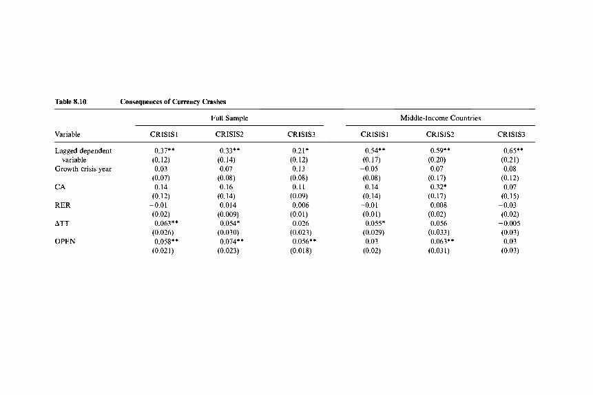
Table 8.10 Consequences of Currency Crashes
Full Sample Middle-Income Countries
Variable CRISIS1 CRISIS2 CRISIS3 CRISIS1 CRISIS2 CRISIS3
Lagged dependent 0.37**
Growth crisis year 0.03 (0.07)
CA 0.14
RER -0.01
ATT 0.063**
OPEN 0.058**
variable (0.12)
(0.12)
(0.02)
(0.026)
(0.021)
0.33** (0.14) 0.07
(0.08) 0.16
(0.14) 0.014
(0.009) 0.054*
(0.030) 0.074**
(0.023)
0.21* (0.12) 0.13
(0.08) 0.1 1
(0.09) 0.006
(0.01) 0.026
(0.023) 0.056**
(0.018)
0.54** (0.17)
(0.08) 0.14
(0.14) -0.01
-0.05
(0.01) 0.055*
(0.029) 0.03
(0.02)
0.59** (0.20) 0.07
(0.17) 0.32*
(0.17) 0.008
(0.02) 0.056
(0.033) 0.063**
(0.031)
0.65** (0.21) 0.08
(0.12) 0.07
(0.15) -0.03 (0.02)
-0.005 (0.03) 0.03
(0.03)
DEBTY
RINT
OT
GDP
INV
R2 N
-0.010 (0.01 1)
-0.06 (0.17)
(0.17) -0.13
-4.OE-5 (5.1E-4)
(0.10)
0.35 85
-0.09
-0.012 (0.012)
-0.12 (0.21)
-0.17 (0.18)
~ 3.5E-4 (6.2E-4)
-0.07 (0.13)
0.39 69
-0.01 1 (0.009) 0.12
(0.15) -0.17* (0.10)
-4.1E-4 (6.5E-4 j 0.02
(0.09)
0.40 80
-0.006 (0.01)
-0.04 (0.21)
6.4E-5 (3.2E-4)
(0.09)
0.47 53
-0.23**
-0.017 (0.016)
(0.26) -0.17
-5.5E-5 (4.3E-4)
(0.13)
0.55 37
-0.25*
-0.014 (0.0 1 4)
(0.22) -0.003
1.2E-4 (4.4E-4)
-0.23** (0.11)
0.56 42
Note: Dependent variable is average output growth after a currency crash, a three-year average, expressed as deviation from the OECD average during the same period. Estimation by OLS with White’s correction for heteroskedasticity. Numbers in parentheses are standard errors. The explanatory variables CA and INV are averages over the three years preceding the event; the variables OPEN, GDP, RER, OT, and DEBTY are levels the year before the event; the variable ATT is the percentage change in the average level of the terms of trade between the period after and the period before the event. *Statistically significant at the 90 percent level. **Statistically significant at the 95 percent level.
Table 8.11 Currency Crashes and Reversals
A. Number of Reversals Preceded by Currency Crashesd
Size of Reversal
No Window Window
Total CRISISl CRISIS2 CRISIS3 CRISISl CRISIS2 CRISIS3 CRISIS4
3%, full sample 152 54 43 51 3%, window, full sample 100 31 26 33 24 3%, window, middle-income
countries 41 18 14 21 14 5%, full sample 117 43 36 43 5%, window, full sample 77 25 22 27 20
B. Growth before and after Reversalsh
Growth before Reversal‘ Growth after Reversald Size of Reversal Total and Type of Crisis Observations Average Median Average Median
3% 97 3.5 3.2 3.6 3.6 3% + CRISISl 30 2.7 2.9 3.1 3.1 3%, no CRISIS1 67 3.9 3.6 3.8 4.1 3% + CRISIS3 32 3.4 3.1 3.5 2.8 3Y0, no CRISIS3 65 3.6 3.3 4.0 3.6
’Number of reversals accompanied by currency crashes or preceded in at least one of the three previous years by crashes. The current account is defined net of official transfers. bReversals do not include adjacent events and are defined on the basis of the current account net of official transfers. They are divided into those accompanied or preceded by currency crises (in one of the previous three years) and those that are not. See table 8.6 note for definitions of CRISISl and CRISIS3. <Growth before reversal: average (median) growth the three years prior to a reversal. “Growth after reversal: average (median) growth rate the year of the reversal and the two successive years.
Current Account Reversals and Currency Crises 317
reversal and in the two preceding years is around 7 percent, well below all the thresholds we use for currency crashes.15 We now investigate this issue in more detail.
A first stylized fact is that as expected, when crises precede or accom- pany reversals they tend to occur one or two years prior to reversals. A second stylized fact is that reversals are more likely to be preceded by currency crises in Latin America and the Caribbean than they are in Asia. For example, for the Frankel-Rose definition of crisis, twelve reversals (out of twenty-five) in Latin America were preceded by crashes, but only five (out of twenty-nine) in Asia.16 If the definition of crisis is changed so as to exclude countries that had high rates of depreciation before crashes (i.e., we use CRISIS3), the numbers change (nine out of twenty-five for Latin America and six out of twenty-nine for Asia) but not the qualitative finding. For African countries, around 30 percent of reversals are pre- ceded by crises. There are more similarities between the stylized features of reversals and crises for the sample of middle-income countries (see the exchange rate depreciation panel in fig. 8.2 and the current account panel in fig. 8.4). However, as shown in the third row of table 8.11, panel A, the fraction of reversals preceded by exchange rate crashes is still below 50 percent. In order to shed more light on this issue it would be necessary to “classify” reversals according to their most relevant features-a task for future research.
The final question we briefly address is whether countries that suffer currency crises prior to reversals tend to perform less well after the rever- sals. Table 8.1 1, panel B, provides summary statistics for median and aver- age growth before and after reversals, separating those preceded by crises from those that are It shows that average and median growth perfor- mance after reversals is worse for countries that suffered currency crises of type 1, but not for crises of type 3. The explanation for this finding may lie in the worse growth performance of countries that suffered bouts of high inflation and currency depreciation (which are excluded from crises of type 3).
8.9 Concluding Remarks
This paper has provided a broad-brush characterization of sharp reduc- tions in current account deficits and of currency crises in low- and middle- income countries. Reversals in current account imbalances are more likely
15. The crisis definition does not affect significantly the selection of reversal episodes pre-
16. This partly reflects the higher incidence of crashes in Latin America than in Asia
17. Table 8.1 1, panel B, excludes CRISISZ; growth would be intermediate between
ceded by crises.
(table 8.6).
CRISIS1 and CRISIS3.

318 Gian Maria Milesi-Ferretti and Assaf Razin
to occur in countries that have run persistent deficits and that have low reserves and unfavorable terms of trade; they are less likely to occur in countries that receive high official transfers and whose debt is largely on concessional terms. Growth performance after reversals tends to be better in more open economies and in countries whose real exchange rates were less appreciated prior to the reversals. Reversals are not systematically associated with declines in growth; indeed, median growth after a reversal in the current account is the same as before the reversal. Currency crises are more likely to occur when reserves are low, real exchange rates are appreciated, and external conditions are unfavorable-high interest rates and low growth in industrial countries. Growth tends to decline the year of the crisis and to recover thereafter. Economies more open to trade seem to perform better after crises. A comparison of currency crashes and cur- rent account reversals shows that these are, in general, distinct events. Less than a third of all reversals are preceded by currency crises, however de- fined. This suggests that the conventional wisdom that large nominal de- preciations precede turnarounds in the current account is not accurate and points to the need to look more closely at different types of reversals.
Several other questions remain open for future research. First of all, the probit analyses of both reversals and currency crises is based on a reduced- form approach that makes it difficult to give any “structural” interpreta- tion to its findings. It would therefore be important to devise ways to dis- tinguish empirically between different mechanisms underlying reversals and crises. A second important question is whether swings in the current account are merely a reflection of reversals in capital flows; addressing this question requires the construction of a measure of capital flows, combin- ing current account and reserve data, taking into account the need to separate “rescue packages” from “normal” capital inflows. Finally, the be- havior of economic policy around the time of reversals and crises could be examined in more detail, and the experience of developing countries could be compared to the experience in industrial countries.
Appendix A
List of Countries
Algeria* Argentina* Bangladesh Barbados Belize Benin
Bhutan Cameroon Bolivia* Cape Verde Botswana* Central African Brazil* Republic Burkina Faso Chad Burundi Chile*
Current Account Reversals and Currency Crises 319
China Colombia* Comoros Congo Costa Rica* C6te d’Ivoire* Djibouti Dominican Republic* Ecuador*
El Salvador* Equatorial Guinea Ethiopia Fiji Gabon Gambia Ghana Grenada Guatemala* Guinea Guinea Bissau Guyana Haiti Honduras Hungary* India Indonesia* Iran* Jamaica* Jordan
Egypt*
Kenya Korea* Laos Lebanon Lesotho Liberia Madagascar Malawi Malaysia* Maldives Mali Malta Mauritania Mauritius* Mexico* Morocco* Myanmar Nepal Nicaragua Niger Nigeria Oman* Pakistan Panama* Papua New
Guinea Paraguay* Peru* Philippines* Portugal*
*Indicates a middle-income country.
Appendix B Data Sources and Definitions
Romania* Rwanda Sgo Tome and Principe Senegal Seychelles Sierra Leone Solomon Islands Somalia South Africa* Sri Lanka* St. Vincent and the
Sudan Swaziland Syria* Tanzania Thailand* Togo Trinidad and Tobago* Tunisia* Turkey* Uganda Uruguay* Vanuatu Venezuela* Western Samoa Yemen Zaire Zambia Zimbabwe
Grenadines
CA Current account balance (excluding official transfers) as a fraction of GDP. Source: World Bank, World Tables and World Development Indicators (Washington, D.C., various issues)-hereafter World Tables.
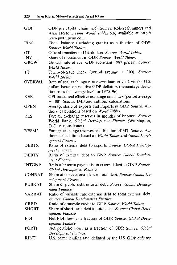
320 Gian Maria Milesi-Ferretti and Assaf Razin
GDP
FISC
OT INV GROW
TT
OVE RVA L
RER
OPEN
RES
RESM2
DEBTX
DEBTY
INTGNP
CONRAT
PUBRAT
VARRAT
CRED SHORT
FDI
PORTF
RINT
GDP per capita (chain rule). Source: Robert Summers and Alan Heston, Penn World Tables 5.6, available at http:// www.pwt.upenn.edu. Fiscal balance (including grants) as a fraction of GDP. Source: World Tables. Official transfers in U.S. dollars. Source: World Tables. Share of investment in GDP. Source: World Tables. Growth rate of real GDP (constant 1987 prices). Source: World Tables. Terms-of-trade index (period average + 100). Source: World Tables. Rate of real exchange rate overvaluation vis-a-vis the U.S. dollar, based on relative GDP deflators (percentage devia- tion from the average level for 1970-96). CPI-based real effective exchange rate index (period average + 100). Source: IMF and authors’ calculations. Average share of exports and imports in GDP. Source: Au- thors’ calculations based on World Tables. Foreign exchange reserves in months of imports. Source: World Bank, Global Development Finance (Washington, D.C., various issues). Foreign exchange reserves as a fraction of M2. Source: Au- thors’ calculations based on World Tables and Global Devel- opment Finance. Ratio of external debt to exports. Source: Global Develop- men t Finance. Ratio of external debt to GNP. Source: Global Develop- ment Finance. Ratio of interest payments on external debt to GNP. Source: Global Development Finance. Share of concessional debt in total debt. Source: Global De- velopment Finance. Share of public debt in total debt, Source: Global Develop- ment Finance. Ratio of variable rate external debt to total external debt. Source: Global Development Finance. Ratio of domestic credit to GDP. Source: World Tables. Share of short-term debt in total debt. Source: Global Devel- opment Finance. Net FDI flows as a fraction of GDP. Source: Global Devel- opment Finance. Net portfolio flows as a fraction of GDP. Source: Global Development Finance, U.S. prime lending rate, deflated by the U.S. GDP deflator.
Current Account Reversals and Currency Crises 321
Source: IMF, International Financial Statistics (Washing- ton, D.C., various issues). Real growth rate in OECD countries. Source: International Financial Statistics. Dummy variable taking the value one if the exchange rate is fixed or fluctuates within a narrow band, and zero other- wise. Source: Cottarelli and Giannini (1997) and IMF, Ex- change Arrangements and Exchange Restrictions (Washing- ton, D.C., various issues). Dummy variable taking the value one if the country has an IMF program in place for at least six months during the year, and zero otherwise. Source: Cottarelli and Giannini (1997).
GROECD
PEG
IMF
References
Calvo, Guillermo A. 1997. Varieties of capital market crises. In The debt burden and its consequences for monetary policy, ed. G. A. Calvo and Mervyn King. New York: St. Martin’s.
Calvo, Guillermo A., Leonardo Leiderman, and Carmen M. Reinhart. 1993. Capi- tal inflows and real exchange rate appreciation in Latin America: The role of external factors. ZMF Staf Papers 40 (March): 108-51.
Calvo, Guillermo A., and Enrique Mendoza. 1999. Rational contagion and the globalization of securities markets. NBER Working Paper no. 71 53. Cambridge, Mass.: National Bureau of Economic Research, June.
Chang, Roberto, and Andris Velasco. 1998. Financial crises in emerging markets: A canonical model. NBER Working Paper no. 6606. Cambridge, Mass.: Na- tional Bureau of Economic Research, June.
Corbo, Vittorio, and Leonardo Hernandez. 1996. Macroeconomic adjustment to capital inflows: Lessons from recent East Asian and Latin American experience. World Bank Research Observer 11 (February): 61-85.
Cottarelli, Carlo, and Curzio Giannini. 1997. Credibility without rules? Monetary frameworks in the post-Bretton Woods era. IMF Occasional Paper no. 154. Washington, D.C.: International Monetary Fund, December.
Debelle, Guy, and Hamid Faruqee. 1996. What determines the current account? A cross-sectional and panel approach. IMF Working Paper no. 96/58. Washing- ton, D.C.: International Monetary Fund, June.
Demirguq-Kunt, Ash, and Enrica Detragiache. 1998. The determinants of banking crises in developed and developing countries. IMF Staf Papers 45 (March): 81-109.
Diamond, Douglas W., and Philip H. Dybvig. 1983. Bank runs, deposit insurance, and liquidity. Journal of Political Economy 91 (June): 401-19.
Edwards, Sebastian. 1989. Real exchange rates, devaluation and adjustment. Cam- bridge, Mass.: MIT Press.
Eichengreen, Barry, Andrew K. Rose, and Charles Wyplosz. 1995. Exchange mar- ket mayhem: The antecedents and aftermatp of speculative attacks. Economic Policy 21 (October): 249-312.

322 Gian Maria Milesi-Ferretti and Assaf Razin
. 1996. Contagious currency crises. CEPR Discussion Paper no. 1453. Lon- don: Centre for Economic Policy Research, August.
Fernandez-Arias, Eduardo. 1996. The new wave of private capital inflows: Push or pull? Journal of Development Economics 48:389-418.
Fernandez-Arias, Eduardo, and Peter Montiel. 1996. The surge in capital inflows to developing countries: An analytical overview. World Bank Economic Review 10 (January): 51-77.
Flood, Robert, and Peter Garber. 1984. Collapsing exchange rate regimes: Some linear examples. Journal of International Economics 17: 1-1 3.
Frankel, Jeffrey A., and Andrew K. Rose. 1996. Currency crashes in emerging markets: An empirical treatment. Journal of International Economics 41 (No- vember): 351-66.
Goldfajn, Ilan, and Rodrigo Valdes. 1997. Capital flows and the twin crises: The role of liquidity. IMF Working Paper no. 97/87. Washington, D.C.: International Monetary Fund, July.
. 1999. The aftermath of appreciations. Quarterly Journal of Economics 104 (February): 229-62.
Jeanne, Olivier. 1997. Are currency crises self-fulfilling? A test. Journal of Znterna- tional Economics 43 (3/4): 163-86.
Jeanne, Olivier, and Paul Masson. 2000. Currency crises, sunspots, and exchange rate regimes. Journal of International Economics 50 (2): 327-50.
Kaminsky, Graciela, Saul Lizondo, and Carmen M. Reinhart. 1998. Leading indi- cators of currency crises. IMF StafSPapers 45 (March): 1-48.
Kaminsky, Graciela, and Carmen M. Reinhart. 1999. The twin crises: The causes of banking and balance of payments problems. American Economic Review 89 (June): 473-500.
Klein, Michael W., and Nancy P. Marion. 1997. Explaining the duration of exchange-rate pegs. Journal of Development Economics 54 (December): 387- 404.
Knight, Malcolm A,, and Julio A. Santaella. 1997. Economic determinants of IMF financial arrangements. Journal of Development Economics 54 (2): 405-36.
Kraay, Aart, and Jaume Ventura. 2000. Current accounts in debtor and creditor countries. Quarterly Journal of Economics, forthcoming.
Krugman, Paul. 1979. A model of balance-of-payments crises. Journal of Money, Credit, and Banking 11 (August): 309-25.
. 1996. Are currency crises self-fulfilling? In NBER macroeconomics annual 1996, ed. Ben S. Bernanke and Julio J. Rotemberg. Cambridge, Mass.: MIT Press.
. 1999. Balance sheets, the transfer problem, and financial crises. In Interna- tionaljnance andJnancia1 crises: Essays in honor of Robert P: Flood, J r , ed. Peter Isard, Assaf Razin, and Andrew K. Rose, 31-44. Boston: Kluwer.
Lane, Philip, and Roberto Perotti. 1998. The trade balance and fiscal policy in the OECD. European Economic Review 42 (May): 887-95.
Masson, Paul. 1998. Contagion: Monsoonal effects, spillovers, and jumps between multiple equilibria. IMF Working Paper no. 98/142. Washington, D.C.: Interna- tional Monetary Fund, September.
Milesi-Ferretti, Gian Maria, and Assaf Razin. 1996a. Current account sustain- ability. Princeton Studies in International Finance, no. 81. Princeton, N.J.: Princeton University, October.
. 199613. Current account sustainability: Selected East Asian and Latin American experiences. NBER Working Paper no. 5791. Cambridge, Mass.: Na- tional Bureau of Economic Research, October.

Current Account Reversals and Currency Crises 323
. 1998. Sharp reductions in current account deficits: An empirical analysis. European Economic Review 42 (May): 897-908.
Obstfeld, Maurice. 1994. The logic of currency crises. Cahiers Economiques et Mo- nitaires (Bank of France) 43:189-213.
Sachs, Jeffrey. 1981. The current account and macroeconomic adjustment in the 1970s. Brookings Papers on Economic Activity, no. 1:201-68.
. 1982. The current account in the macroeconomic adjustment process. Scandinavian Journal of Economics 84 (2): 147-59.
Sachs, Jeffrey, Aaron Tornell, and AndrCs Velasco. 1996. Financial crises in emerg- ing markets: Lessons from 1995. Brookings Papers on Economic Activity, no.
Santaella, Julio A. 1996. Stylized facts before IMF-supported macroeconomic ad- justment. IMF S t a f Papers 43 (September): 502-44.
Tornell, Aaron, and Philip Lane. 1998. Are windfalls a curse? A non-representative agent model of the current account and fiscal policy. Journal of International Economics 44 (February): 83-1 12.
Wyplosz, Charles. 1986. Capital controls and balance-of-payments crises. Journal of International Money and Finance 5 (June): 167-79.
1 : 147-98.
Comment Jaume Ventura
This is the latest paper in a series by Milesi-Ferretti and Razin (1996a, 1996b, 1998) that has taught us much regarding current account sustain- ability and sharp reductions in current accounts. In this new installment of the saga, the authors also include a description of large depreciation episodes. In this brief comment, I focus on two issues. First, I raise a meth- odological point that I hope the authors interpret as a challenge for their future research. Second, I stress some of the implications of their findings regarding large depreciations.
Section 8.4, on current account reversals, contains a description of how the key macroeconomic variables (with special attention to growth) be- have during a current account reversal.’ In particular, they find that on average these episodes tend to be preceded by unfavorable terms of trade, low foreign exchange reserves, a high interest burden of external debt, low consumption growth, and a high budget deficit. After the sharp reduction in the current account deficit takes place, on average most of these indica- tors improve, although the growth rate remains at roughly the same level
Jaume Ventura is the Pentti Kouri Associate Professor of Economics at the Massachusetts Institute of Technology and research associate of the Centre for Economic Policy Re- search, London.
1. Section 8.4 also contains an attempt to use multivariate probit analysis to find good indicators of current account reversals. However, this effort is marred by the use of the cur- rent account variable as a regressor. This variable was used to construct the dependent vari- able, and as a result, it cannot be used as an explanatory variable. 1 suspect that the numbers might change substantially if the probit analysis were properly executed.


![Currency crises · 2018-04-04 · Currency crises Tomasz Michalski1 1GREGHEC: HEC Paris [International Macroeconomics] Typology of currency crisis models First-generation models Second-generation](https://img.dokumen.tips/doc/110x75/5edacb4da22bb1624d6d8fc0/currency-crises-2018-04-04-currency-crises-tomasz-michalski1-1greghec-hec-paris.jpg)