Current Account and Real Exchange Rate changes: the impact …€¦ · Current Account and Real Exchange Rate changes: the impact of Trade Openness Davide Romelli Universit e de Cergy-Pontoise,

Current Account and Real Exchange Rate changes:

the impact of Trade Openness

Davide RomelliUniversite de Cergy-Pontoise, THEMA

Cristina TerraUniversite de Cergy-Pontoise, THEMA

Enrico VasconcelosBanco Central do Brasil

November 25, 2013

This draft: November 2013First draft: February 2013

Abstract

This article investigates the impact of trade openness on the rela-tion between real exchange rate depreciation current account. First,using data for developed and emerging economies for the period 1970–2011, we identify events of sudden stops of capital flows and of abruptreal exchange rate depreciations. Then, we investigate the relationbetween openness, real exchange rate depreciations, and changes incurrent account and in trade balance over those events. We find that,controlling for real exchange rate changes, more open economies ex-perience a larger increase in current account and in trade balance. Inother words, our results indicate that improvements in current accountand in trade balance are accompanied by smaller real exchange ratedepreciation in more open economies.

Keywords: trade openness, sudden stops, real exchange rate depre-ciation.JEL classification: F32, F37.

1 Introduction

Both advanced and emerging economies have experienced exponential growthof capital flows over the past twenty years. On the years 2000s, this growthwas accompanied very large and mounting current account imbalances, rais-ing concerns with respect to the potential adverse consequences of abruptinterruptions of those flows and current account reversals. In particular,the magnitude of exchange rate depreciation over the adjustment processhas been an important element in the debate, reviving the famous debate

1

between John Maynard Keynes and Bertil Ohlin over the payment of wardebts in Germany during the 1920s, known as the “Transfer Problem”.

In the transfer problem debate, Keynes argued that, in order to pay forthe war damages in foreign currency, Germany would have to raise the re-sources through trade balance surpluses. Relative prices of tradable goodswould then have to fall, implying a terms of trade deterioration and cur-rency depreciation. According to Ohlin, however, the decline in Germany’sdisposable income due to the external payments would entail an increasein trade balance with lesser relative price changes. The mechanism is that,with lower income, the country would buy less of “the goods which go eas-ily between them”, using Ohlin’s words, thereby improving trade balance.Clearly, the efficiency of this mechanism depends on the share of those goodsin the consumption basket, that is, on the degree of openness of the economy.

The reversion of large current account imbalances refers to the sametype of adjustment mechanism, where the magnitude of real exchange ratedepreciation may be mitigated by the income effect, particularly in moreopen economies. We take this question to the data: do more open economiesendure lesser real exchange rate depreciation when facing current accountreversals? Many different variables affect the relation between real exchangerates and trade balances, and it would be a daunting, if not impossible taskto control for all of them. To circumvent this problem, we focus our analysison episodes of sudden stops of financial flows and of abrupt changes in realexchange rates. In the case of sudden stops, it is reasonable to think that,on average, other shocks affecting trade balance and real exchange rateswould assume a lesser role, so that the observed real exchange rate changewould be associated to the trade balance movement. By the same token,in events of abrupt exchange rate depreciation, the corresponding change intrade balance can be taken as mostly related to the observed exchange ratedepreciation.

Empirical research recognizes the importance of openness to trade in de-termining the country’s vulnerability to sudden stops. For example, Calvo,Izquierdo, and Mejia (2004) present evidence that more open economies,understood as countries with larger supply of tradable goods, are less proneto sudden stops in capital flows. Cavallo and Frankel (2008), on their turn,show how this relationship is even stronger when taking into account theendogeneity of openness to trade measure.

The currency crises literature equally stresses the importance of tradeopenness. Examining the factors that help predict the occurrence of theseextreme episodes, Milesi-Ferretti and Razin (2000) find that an higher de-gree of openness to trade decrease the probability of exchange rate crashes.Moreover, they also show how more open economies are characterized bya faster growth in the aftermath of a currency crisis. Similar findings arepresented in Glick and Hutchison (2011), where greater trade integrationreduces a country’s financial fragility and the likelihood of a currency crisis

2

by increasing both the ability and willingness to service external obligations.Indeed, a greater export ratio decreases the likelihood of sharp reversals ofcapital flows, as the country is more able to service its foreign currencydenominated debt.

All in all, the literature has established the importance of trade opennessin the country’s vulnerability to sudden stops and currency crises. We takea new perspective by investigating the role of trade openness on the relation-ship between trade balance and real exchange rate during these episodes.More specifically, we analyze the role played by trade openness on the rela-tion between trade balance and real exchange rate during sudden stops andabrupt real exchange rate depreciation episodes, for advanced economies andemerging markets.

We build a theoretical framework that captures the role of trade opennesson the relation between current account reversals and real exchange ratechanges. We model a small open economy in which sudden stops can occurdue to binding collateral constraints on the country’s external debt. Weshow that the effect of this sudden stop differs according to the degree ofopenness of the economy. In particular, more open economies experience alower exchange rate depreciation.

We then examine the empirical implications of this model for a sampleof both advanced and emerging economies during the period 1970–2011.We first identify sudden stops and abrupt real exchange rate depreciationepisodes by following a standard methodology used in the sudden stopsliterature.

We show that during sudden stops more open economies endure lowerdepreciation of the real exchange rate. We also provide evidence that tradeopenness has a positive impact on trade balance and current account varia-tions during episodes of sudden stops and of abrupt exchange rate depreci-ation. The direct implication of these findings is that more open economiesseem to be able to reach equilibrium in the balance of payments with lowerreal exchange rate depreciation.

The outline of the paper is as follows. In Section 2 we present a theoret-ical framework that establishes how openness affects exchange rate depreci-ation under sudden stops. Section 3 describes the data, while the empiricalresults are presented in Section 4. Section 5 concludes.

2 Theoretical Framework

This section present a simple theoretical framework that shows how, dur-ing sudden stops, more open economies experience lesser real exchange ratedepreciations. The formal specification of the model follows the small openeconomy literature with tradable and nontradable goods sectors (see Men-doza, 2005; Bianchi, 2011; Korinek and Mendoza, 2013).

3

2.1 Set-up

The economy is populated by a continuum of identical households thatreceive in every period an endowment of tradable (yTt ) and nontradable(yNt ) goods. They allocate their consumption (Ct) between those two goodsgoods, by maximizing the following expected utility function:

U =∑

βtE [u (Ct)] , (1)

where β is the discount factor and ct is the consumption basket. For sim-plicity, we assume Cobb-Douglas preferences, so that:

Ct =(cTt)γ (

cNt)1−γ

, (2)

where γ is the share of tradable goods in consumption.Households can invest in a foreign asset denominated in units of tradable

goods. This asset matures in one period and pays a fixed gross interest rateR. Taking the price of tradables as the numeraire and denoting as pNt theprice of nontradables, the household’s budget constraint can written as:

bt+1 + cTt + pNt cNt = yTt + pNt y

Nt +Rbt, (3)

where bt+1 represent the amount of bonds held by the household at time t.Notice that debtor countries present a negative value of b.

We assume that this economy faces a borrowing constraint. More specif-ically, we assume foreign creditors restrict the loans to the country so thatthe amount of debt cannot exceed a fraction k of tradable income. In thiscase, the credit constraint is represented by:

bt+1 ≥ −kyTt . (4)

The market clearing condition in the nontradables sector is given by:

cNt = yNt , (5)

which we substitute into the budget constraint in equation (3) to rewrite itas:

cTt = yTt +Rbt − bt+1. (6)

We are interested in investigating the impacts of sudden stops, whichwe will represent as a shock to the tradable good endowment in a creditconstrained economy, as in Mendoza (2005). Hence, we start by describingthe equilibrium when the credit constraint in not binding, and then weanalyze the effect of a shock to the tradable endowment (yTt ). Finally, weshow how the effect of a sudden stop differs according to the degree ofopenness of the economy.

4

2.2 Non-binding credit constraint

For simplicity, we assume that the nontradable output is constant over time,yNt = yN for all t, and that βR = 1. Given these assumptions, when thecredit constraint does not bind the equilibrium simply reflects the perfectconsumption smoothing of tradable goods: cTt = cT for all t. Assuming theno-Ponzi game condition, the intertemporal budget constraint (6) impliesthe following value for the constant tradables consumption:

cT =

(R− 1

R

)( ∞∑t=0

R−tyTt +Rb0

)(7)

Consumers maximize utility when relative price of nontradables is equalto the marginal rate of substitution between the two types of goods. Theequilibrium price of nontradables is then given by:

pNt =

(1 − γ

γ

)cTtcN, (8)

which is constant at pN in this case with non binding credit constraint.Defining the real exchange rate ε as the ratio between the price of trad-

able goods, our numeraire, and the price of nontradables (pN ), we have thatεt = 1

pNt. Hence, it is also constant (ε) in this unconstrained economy.

Let us see the effect of a negative shock to the tradable endowment,. Wewill construct a wealth neutral shock, so that it should not affect consump-tion paths when the credit constraint in equation (4) is not binding. Follow-ing Mendoza (2005), we first define a sequence of time invariant tradablesendowment (yT ) that yields the same present value of the actual arbitrarytime varying sequence of tradables income. According to this definition,tradables consumption under no credit constraints from equation (7) can bewritten as:

cT = yT + (R− 1) b0. (9)

Let us suppose that current account is balanced when the economy ishit the wealth neutral negative shock. It is defined as a negative shock totradables income at date 0 that is offset by positive shock at date 1, so thatthe present value of the tradable output remains unchanged. In order tokeep the present value of the sequence of the tradables income constant, theendowment shock needs to satisfy the following condition:(

yT − yT0)R = yT1 − yT . (10)

If the shock to yT0 is not large enough to trigger the credit constraint,consumption allocation and the price of nontradables remain unchanged.

5

Indeed, at date 0 the country will consume the same level of tradables,cT0 = cTt , thanks to the increased foreign debt:

b1 − b0 = yT0 − yT < 0. (11)

At date 1, the positive shock that offsets the one occurred at date 0 willallow the country to maintain a constant consumption and to reimburse theincrease in debt of the previous period, so that b2− b1 = −

(b1 − b0

). In such

a situation, the effect of the shock is only reflected on the current account,with the country facing a deficit at date 0 and a surplus at date 1.

2.3 Binding credit constraint: sudden stop episode

We now analyze the impacts of an unanticipated shock to the endowmentof tradable goods that triggers the liquidity constraint, that is, a shock thatwould induce a debt level b1 that does not satisfy the credit constraint inequation (4), so that b1 < −kyT0 . Notice that, given the change in debtinduced by the endowment shock in equation (11), it must be the case that:

yT0 <yT − b01 + k

. (12)

In this case, equation (4) is binding, so that:

b1 = −kyT0 > b1. (13)

where b1 is the indebtedness level that would be necessary to keep consump-tion constant, as defined in the previous subsection. The consumption oftradables at date 0 is then given by:

cT0 = (1 + k) yT0 +Rb0. (CC) (14)

which is clearly smaller that the original consumption smoothing plan: cT0 <cT .

The price of nontradables is now equal to:

pN0 =

(1 − γ

γ

)cT0cN

< pN , (15)

which is then lower than the unconstrained level, which means a more de-preciated real exchange rate: ε0 > ε

Notice that, with the binding credit constraint, the current account islarger than in the case of the unconstrained economy:

b1 − b0 > b1 − b0, (16)

6

since b1 > b1, by construction. Furthermore, the change the difference be-tween the two value of the current account is captured by the drop in con-sumption. Using equation (6) to compute consumption when the endowmentis equal to yT0 , and equation (9) for the consumption in the unconstrainedeconomy, we have that:

cT − cT0 = (b1 − b0) −(b1 − b0

), (17)

In sum, when an unanticipated shock triggers the credit constraint tobind, which represents a sudden stop episode, the consumption of tradablegoods decreases, the real exchange rate depreciates, and the current accountdeficit is smaller than it would be under no credit constraint.

2.3.1 The importance of Openness

We define the degree of openness of an economy as the share of tradablegoods in consumption, which, given consumer preferences represented inequation (2), can be expressed as:

Opennesst =cTt

pNt cN + cTt

= γ. (18)

Consider two economies, denoted O and C, differing on their degree ofopenness, with γO > γC , i.e., O is more open than C. Both economies havethe same constant endowment of nontradable goods. As for the tradablesendowment, its present value is larger in the more open economy, and thedifference is such that the real exchange rate is the same in the two economieswhen they are not credit constrained. From equations (8) and (9), thecondition is that:

yTO =γO (1 − γC)

γC (1 − γO)

(yTC + (R− 1)b0C

)− (R− 1)b0O. (19)

Suppose these economies are initially both consuming at the uncon-strained consumption level with balanced current account, when they are hitby an unexpected, wealth-neutral, negative shock in tradables endowmentthat triggers the budget constraint. What will be the effect on the tradableconsumption, nontradable prices and real exchange rate?

Since the shock is wealth-neutral, the negative shock at date 0 is com-pensated in each economy by a positive shock in period 1 satisfying the con-dition in equation (10). Moreover, in order to trigger the credit constraint,tradable endowment must satisfy inequality (12). Finally, to facilitate thecomparison between the two economies, we assume that the the shocks in-duce the same decrease in tradables consumption. Hence, they satisfy the

condition: yT0O − yT0C =yTO−y

TC

1+k .

7

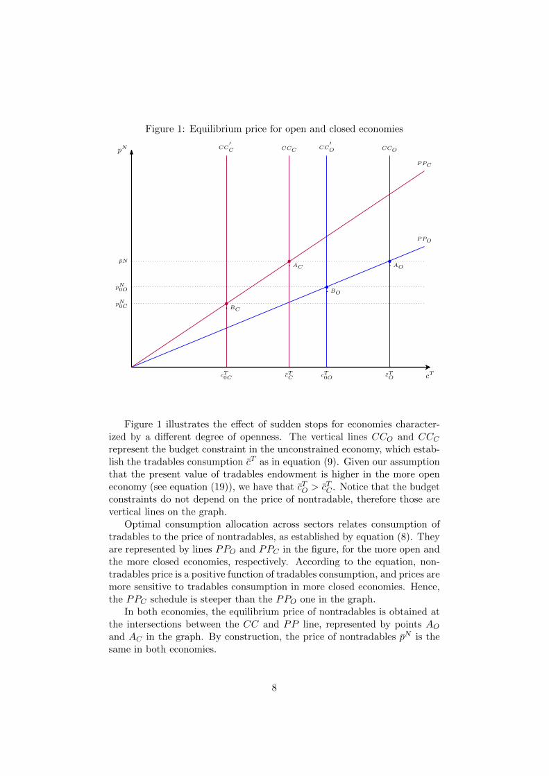
Figure 1: Equilibrium price for open and closed economies

cT

pN CCOCCC

PPO

PPC

pN

cTOcTC

AC AO

CC′O

cT0O

pN0O BO

CC′C

cT0C

pN0C BC

Figure 1 illustrates the effect of sudden stops for economies character-ized by a different degree of openness. The vertical lines CCO and CCCrepresent the budget constraint in the unconstrained economy, which estab-lish the tradables consumption cT as in equation (9). Given our assumptionthat the present value of tradables endowment is higher in the more openeconomy (see equation (19)), we have that cTO > cTC . Notice that the budgetconstraints do not depend on the price of nontradable, therefore those arevertical lines on the graph.

Optimal consumption allocation across sectors relates consumption oftradables to the price of nontradables, as established by equation (8). Theyare represented by lines PPO and PPC in the figure, for the more open andthe more closed economies, respectively. According to the equation, non-tradables price is a positive function of tradables consumption, and prices aremore sensitive to tradables consumption in more closed economies. Hence,the PPC schedule is steeper than the PPO one in the graph.

In both economies, the equilibrium price of nontradables is obtained atthe intersections between the CC and PP line, represented by points AOand AC in the graph. By construction, the price of nontradables pN is thesame in both economies.

8

With the tradable endowment shock that triggers the credit constraint,consumption is given by equation (14), represented by the vertical lines CC ′Oand CC ′C . The new equilibrium is at point BO for the more open economyand at point BC for the more closed one.

Despite the fact that the change in the consumption of trabables is equalfor both economies (∆cTO = ∆cT0C), the more closed economy exhibits alarger decrease on the relative price of nontradable goods. This imply thatthe shock to the tradables endowment at date 0 generates a larger realexchange rate depreciation for the less open economy. Thus, during suddenstops, for a given variation of the current account, more open economiesendure a lower real exchange rate depreciation.

Going back to the Keynes-Ohlin debate, we could say, in light of thisargument, that Ohlin would be right for economies with a high degree ofopenness. The credit constraint that is triggered by the endowment shockdecreases the disposable income, depressing consumption of both types ofgoods. Nontradables prices have then to decrease to reestablish equilibriumin the nontradables market. The more open the economy, the larger is thedecrease in total tradables consumption and the smaller the decrease innontradables consumption for a given decrease in available income. Hence,the lesser the relative price changes.

We investigate whether the data meets this argument. More specifically,we verify whether real exchange rate depreciations are smaller in more openeconomies when they are hit by sudden stops. We also look at the issuefrom the opposite perspective, that is, in events of large real exchange ratedepreciations, whether the increase current accounts and trade balances arelarger in more open economies.

3 Event analysis and data

The first step is to identify sudden stops and exchange rate depreciationepisodes, which are the events in which our empirical investigation will bebased. We use quarterly data from the IFS-IMF database for a sample of128 developed and emerging economies for the period 1970-2011. Noticethat we do not have data for all countries and all periods, so that we maymissed some of the episodes of abrupt RER depreciation and sudden stopsthat actually occurred over the period.

3.1 Sudden stop episodes

We identify sudden stops by adapting the methodology implemented byCalvo et al. (2004) to quarterly data. We define an episode as a suddenstop when the year-over-year change of quarterly net capital flows falls twostandard deviation below its mean. As common in the literature, we set thebeginning of the sudden stops as the first quarter in which the fall in capital

9

flows is larger than one standard deviation below its mean and end once thefall in net capital flows is smaller than one standard deviation.

In line with Calvo et al. (2004), and contrary to other studies (i.e.Guidotti et al., 2004; Edwards, 2004; Calderon and Kubota, 2013), we donot normalize the changes in capital flows by GDP or exclude the episodesfor which the shock does not exceeds a certain threshold of GDP. By limitingsudden stops episodes to events for which the change in net capital flowsexceed a certain threshold (for example Guidotti et al., 2004, fix this thresh-old at 5% of GDP), we might exclude episodes that occurred in countriescharacterized by a low capital flows volatility or by less open economies.

Our methodology differs from Calvo et al. (2004) in three main aspects.First, we measure capital flows on a quarterly, rather than on a yearlybasis and compute the year-over-year changes to avoid seasonal fluctuations.Second, we compute the 3 years moving average and standard deviation ofcapital flows and not their historical average and standard deviations. Bylimiting the time horizon for the computation of the mean and the standarddeviation, we provide a better instrument to detect “unexpected” reductionsin net capital flows. Finally, whenever we identify two sudden stops episodesseparated by only one quarter, we consider them as a unique episode.

We proxy the capital inflows k of country c in quarter q as the quarterlychange in international reserves IR minus the quarterly current accountCA:1

kc,q = (IRc,q − IRc,q−1) − CAc,q. (20)

The year-over-year changes in capital flows are simply defined as ∆kc,q =kc,q−kc,q−4. We then identify sudden stops whenever the following conditionis met:

∆kc,q < µ(∆kc,q) − 2σ(∆kc,q), (21)

where µ and σ represent the three years moving average and standard de-viation, respectively.

As an example, the grey areas in Figure 2 depicts the sudden stopsidentified for Brazil from 1979 to 2011. The solid line plots ∆kc,q, whilevalues that lays two (one) standard deviations below the three years movingaverage are depicted by the dashed (short dashed) line. During this period,Brazil experienced five sudden stops.

Using this methodology we identify, during the period 1970-2011, 329sudden stop episodes for a sample of 128 countries: 205 of them occurred inemerging markets and developing countries (as classified by the IMF WorldEconomic Outlook) and 124 in advanced economies. Figure 3 shows thedispersion of sudden stops across countries. Before the 1990s, however, there

1All series are measured in constant 2005 dollars.

10

Figure 2: Sudden stops in Brazil, 1981-2011−4

0−2

00

2040

Capi

tal I

nflo

ws (U

S Bi

llion

$)

1980q1 1985q1 1990q1 1995q1 2000q1 2005q1 2010q1

are missing data for many emerging market economies, which may explainthe relatively few sudden stopes among those countries for the first twentyyears of our sample. For the period 1990–2011, we observe 174 sudden stopsin capital flows among emerging and developing countries and 83 developedeconomies. As expected, these events are much more common in emergingmarkets.

Figure 3: Sudden stop episodes across countries (1970-2011)

Nr of Sudden Stops(4,9](3,4](2,3][1,2]No data

In Figure 4 we observe several sudden stop episodes among advancedeconomies during the European Monetary System crisis (1990 and 1992)and the Asian crisis (1998). In emerging markets these episodes are con-centrated around the Mexican (1994 to 1995), Asian (1997), Russian (1998)

11

Figure 4: Frequency of sudden stops, 1970-20110

510

1520

25N

r of S

udde

n St

ops

1970q1 1975q1 1980q1 1985q1 1990q1 1995q1 2000q1 2005q1 2010q1Quarter

Emerging Markets Advanced Economies

and Argentinean (2001) crises. A large number of sudden stops in bothemerging and developed economies is detected over the late 2000s, in themidst of the world financial crisis.

Calvo et al. (2004) find that more closed economies or those with a higherdegree of dollar denominated debt have a higher probability of experienc-ing sudden stops. Following Rey and Martin (2006), we split our sampleof advanced economies and of emerging markets in terms of their opennessto trade. We measure trade openness as the average over the whole periodof exports plus imports as a ratio of GDP. We then classify as more openeconomies those for which the openness ratio is above the median of itsgroup. Figures 5 and 6 confirm that, indeed, more closed economies expe-rience an higher number of sudden stops among both advanced economiesand emerging markets, during the period 1970-2011.

12

Figure 5: Frequency of sudden stops in advanced economies, 1970-20110

510

15N

r of S

udde

n St

ops

in A

dvan

ced

Econ

omie

s


Closer Economies More Open Economies

Figure 6: Frequency of sudden stops in emerging markets, 1970-2011

05

1015

Nr o

f Sud

den

Stop

s in

Em

erge

rgin

g M

arke

ts


Closer Economies More Open Economies

3.2 Episodes of abrupt real exchange rate depreciation

Little attention has been dedicated in the literature to identifying episodesof abrupt depreciation of both the real exchange rate (RER). Empirical

13

studies in exchange rate variations commonly focus their attention on nomi-nal exchange rate movements and, more specifically, on currency crises (see,among others, Milesi-Ferretti and Razin, 2000; Laeven and Valencia, 2012).

We identify abrupt depreciations of the RER using the same methodol-ogy followed for the identification of sudden stops, described in the previoussubsection. More precisely, a RER depreciation occurs when the year-over-year increase in quarterly real exchange rate is larger than two standarddeviations above its mean. Moreover, the episode window of a RER de-preciation: i) begins once the RER increase in higher than one standarddeviation above the mean; ii) ends when the RER increase falls below onestandard deviation.

The real exchange rate ε of country c in quarter q is measured as thenominal exchange exchange rate2 E, defined as domestic currency per unitof U.S. dollar, multiplied by the ratio between the consumer price index inthe U.S. and in country c:

εc,q = Ec,q ∗CPIUS,qCPIc,q

(22)

We then compute the yearly change of the quarterly RER as: ∆εc,q =ln(εc,q/εc,q−4). Finally, we consider an abrupt RER depreciation as anepisode for which: ∆εc,q > µ(∆εc,q) + 2σ(∆εc,q), where µ and σ representthe three years moving average and standard deviation, respectively.

The RER is a goods measure of the relative price incentives for tradewith the U.S. Countries, however, have several trade partners, and the U.S.is not always the main one. Hence, we also proceed with the identificationof REER depreciation episodes. Indeed, since the REER measures the valueof a currency against a weighted average of foreign currencies, these eventsmight provide a more clear idea of the impact of a depreciation on thetrade balance and the current account of the country. The only drawbackof using these data is that their availability is restricted to a smaller sampleof countries and mainly for a shorter time horizon (from 1995 to 2011).

The IMF defines the REER so that an increase in the value representsa real appreciation of the home currency. To facilitate a comparison of theresults obtained for RER and REER we compute the year-over-year changeof the quarterly REER as ∆REERc,q = ln(REERc,q−4/REERc,q). Con-sequently, a positive variation of the REER represents a real depreciationof the home country. We identify abrupt REER depreciation following thesame methodology used for the identification of RER depreciations.

The gray areas in Figure 7 are the abrupt RER depreciation episodesidentified for Brazil from 1981q1 to 2011q4. The solid line plots ∆RERc,q,while values that lays one and two standard deviations above the three yearsmoving average are depicted by the lower and the upper dashed lines. During

2Exchange rate data is taken from the IMF’s International Financial Statistics (IFS).

14

Figure 7: ∆RER and depreciation episodes in Brazil (1981-2011)−6

5−4

0−1

510

3560

1981q1 1986q1 1991q1 1996q1 2001q1 2006q1 2011q1

this period, Brazil experienced four abrupt RER depreciation episodes. Theabrupt RER depreciation episode that took place from 1998q3 to 1999q4,for example, begins once the change in RER jumps one standard deviationabove the mean (1998q3), overtaking two standard deviations in 1999q1.The episode window ends when the RER variation bounces back to a valuebelow one standard deviation from the mean (1999q4).

Figure 8 presents the same analysis, while looking at REER depreciationepisodes. Comparing the two figures, we see that RER and REER changesfollow the same pattern and the depreciation episodes coincides in almostall cases, but not all of them: the REER presents an abrupt depreciationepisode in 2002 that is not captured the RER. Also, between 1994 and1995, the real appreciation of the Brazilian currency was not followed by anappreciation of the real effective rate. This event could have had a negativeimpact on the bilateral trade between Brazil and the US and only a marginaleffect on the overall values of imports and exports of the country. Hence,although RER does not perfectly reflect REER, it is a reasonable proxy forit.

In a broad set of 64 developed and developing countries, for the pe-riod 1970–2011, we find 295 real exchange rate depreciation episodes and227 real effective exchange rate depreciation events. Figure 9 shows howthese episodes are spread across countries, whereas Figures 10 and 11 de-pict their frequency over time. Comparing these two figures we see a highconcentration of RER depreciations episodes in some periods, while REERdepreciations events are spread over time.

15

Figure 8: ∆REER and depreciation episodes in Brazil (1981-2011)−6

5−4

0−1

510

3560

1981q1 1986q1 1991q1 1996q1 2001q1 2006q1 2011q1

Figure 9: RER depreciation episodes across countries (1970-2011)

Nr of RER depreciations(7,9](5,7](3,5][1,3]No data

4 Empirical results

We investigate the impact of openness to trade on RER depreciation, currentaccount and trade balance during episodes of sudden stops and of abruptRER depreciation. Notice that our empirical analysis in based on crosssection data in which each observation refers to an episode of either suddenstop or abrupt RER depreciation. Our main independent variable is thedegree of trade openness, which we measure as the the sum of goods exportsand imports divided by GDP.

It is worth mentioning that our measure of openness is not exactly thetheoretical definition of openness, which we had defined as the share oftradables in consumption. Literally, tradable goods should be the sum of

16

Figure 10: Frequency of RER depreciation episodes, 1970-20110

2040

6080

Nr o

f RER

dep

reci

atio

ns

1980q1 1985q1 1990q1 1995q1 2000q1 2005q1 2010q1Quarter


all good that could potentially be exported and the imported goods. Weknow, however, that there is a big difference between being potentially ex-ported, and being actually exported. For a potentially exportable good tobe actually exported there are non negligible fixed cost involved, and a fastgrowing literature certifies that these fixed costs do prevent a large fractionof tradable goods to be actually traded. The tradable goods in the theoret-ical model refer to “goods which go easily between [the counties]”, again,paraphrasing Ohlin. Hence, the sum of imports and exports is a good proxyfor this kind of goods.

4.1 Openness, RER depreciation and current account rever-sals during sudden stops

Building on the extensive literature on sudden stops, our goal here is checkthe impact of openness on RER depreciations and trade balance adjustmentduring episodes of sudden stops in capital inflows. We start by lookingat the correlation between openness and RER changes, controlling for theintensity of the sudden stop. We define a pre-episode window as the obser-vations in the year before the beginning of a sudden stop, while an episodewindow is the period that goes from the beginning to the three quartersafter its end. From the episode window, we extract the real and real effec-tive exchange rate variations, whereas the trade openness is measured in thepre-episode window. By using the lagged data (i.e. pre-episode window) oftrade openness, we try to reduce any endogeneity concerns with exchange

17

Figure 11: Frequency of REER depreciation episodes, 1970-20110

1020

30N

r of R

EER

dep

reci

atio

ns

1980q1 1985q1 1990q1 1995q1 2000q1 2005q1 2010q1Quarter


rate variations.In our cross-sectional analysis, some countries may appear more that

once, when they suffer more than one sudden stop over the time range ofour study. Therefore, in all our regressions we relax the assumption of theindependent distribution errors term across time, allowing the clustering ofobservations by country. Consequently, we assume that the error term isi.i.d. across countries but not necessarily for different observations withinthe same economy. All reported standard errors are adjusted for clustering.

Table 1: RER depreciation and openness during sudden stopsDependent Variable: ∆ RER ∆ REER

Openness -0.00044** -0.00228(0.000) (0.000)

∆ Capital Flows -0.00000** -0.00000(0.000) (0.000)

Constant 0.03957* 0.38142(0.020) (0.251)

Observations 285 176Nr of countries 93 60R-squared 0.026 0.099

Robust standard errors in parentheses. ** p<0.05, * p<0.1.

As a first glance at the date, Table 1 shows the result of a simple regres-sion to try to capture the correlation between openness and RER changes

18

in episodes of sudden stops. In line with our expectations, we do find a neg-ative correlation between trade openness and RER changes during suddenstops, while controlling for the change in capital flows, which is a measure ofthe intensity of the sudden stops. When we use the real effective exchangerate, the coefficient of openness is still negative, but not significant. Thedata set is much smaller when we use REER, which could be one possi-ble explanation for these non significant coefficients. These results suggestthat more open economies, when hit by sudden stops, endure a lower realexchange rate depreciation.

One problem with just looking are RER changes is that government in-tervention in the foreign currency market may, at least partially, preventcurrent account adjustment from occurring, and therefore we would observesmaller RER devaluations. If governments in more open countries are, forsome reason, more prone to intervene to prevent depreciations, these inter-ventions could be driving the results, instead of the mechanism described inthe theoretical model.

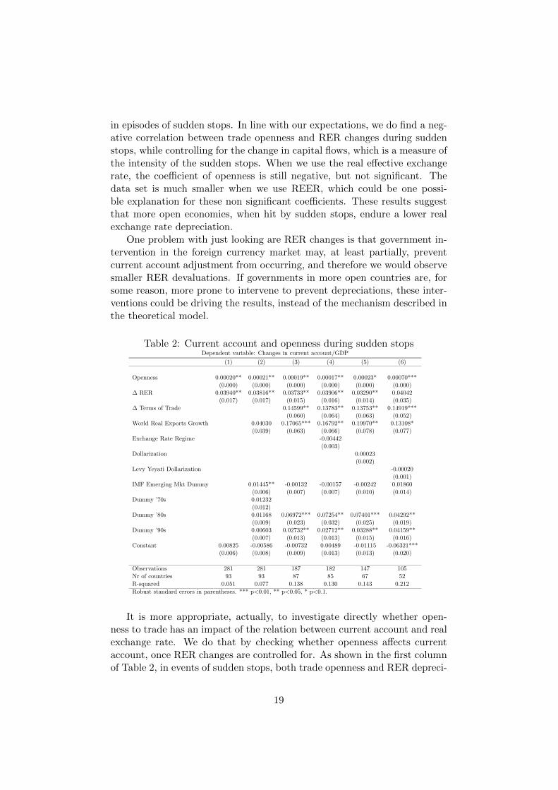
Table 2: Current account and openness during sudden stopsDependent variable: Changes in current account/GDP

(1) (2) (3) (4) (5) (6)

Openness 0.00020** 0.00021** 0.00019** 0.00017** 0.00023* 0.00070***(0.000) (0.000) (0.000) (0.000) (0.000) (0.000)

∆ RER 0.03940** 0.03816** 0.03733** 0.03906** 0.03290** 0.04042(0.017) (0.017) (0.015) (0.016) (0.014) (0.035)

∆ Terms of Trade 0.14599** 0.13783** 0.13753** 0.14919***(0.060) (0.064) (0.063) (0.052)

World Real Exports Growth 0.04030 0.17065*** 0.16792** 0.19970** 0.13108*(0.039) (0.063) (0.066) (0.078) (0.077)

Exchange Rate Regime -0.00442(0.003)

Dollarization 0.00023(0.002)

Levy Yeyati Dollarization -0.00020(0.001)

IMF Emerging Mkt Dummy 0.01445** -0.00132 -0.00157 -0.00242 0.01860(0.006) (0.007) (0.007) (0.010) (0.014)

Dummy ’70s 0.01232(0.012)

Dummy ’80s 0.01168 0.06972*** 0.07254** 0.07401*** 0.04292**(0.009) (0.023) (0.032) (0.025) (0.019)

Dummy ’90s 0.00603 0.02732** 0.02712** 0.03288** 0.04159**(0.007) (0.013) (0.013) (0.015) (0.016)

Constant 0.00825 -0.00586 -0.00732 0.00489 -0.01115 -0.06321***(0.006) (0.008) (0.009) (0.013) (0.013) (0.020)

Observations 281 281 187 182 147 105Nr of countries 93 93 87 85 67 52R-squared 0.051 0.077 0.138 0.130 0.143 0.212

Robust standard errors in parentheses. *** p<0.01, ** p<0.05, * p<0.1.

It is more appropriate, actually, to investigate directly whether open-ness to trade has an impact of the relation between current account and realexchange rate. We do that by checking whether openness affects currentaccount, once RER changes are controlled for. As shown in the first columnof Table 2, in events of sudden stops, both trade openness and RER depreci-

19

ation have a positive and significant effect on current account, as predictedby the theory.

Columns (2) to (6) in the table present the results of regressions addingadditional controls to make sure that the result in column (1) is not beingdriven by omitted variables. We control for terms of change and worldexports growth, since these two variables would have a direct impact ontrade balance. Terms of trade variation might be subject to endogeneityissues, so we take is average change in the pre-episode window. Worldexport growth, on its turn, should not be endogenous to a specific countrysudden stop episode, so we compute its average during the episode window.The coefficient for both variables is positive and significant, as expected:improvements in the terms of trade and higher world exports have a positiveimpact on trade balance, thus increasing the current account balance.

We add a dummy for emerging markets to capture possible differencebetween developed and emerging economies. These two type of economiesdiffer in a number of ways, including the level of external debt, risk, tradepatterns, among others, which could potentially affect how their currentaccounts respond to RER changes. We also control for time with threedecade dummies, for the 1970s, 1980s and 1990s.

The impact of the emerging markets dummy is positive and significantin column (2), where terms of trade and 1970s dummy are not included.In all other regression its coefficient is not significantly different from zero.Notice that, due to lack of data, the 1970s data contains mostly developedcountry, as can be seen in Figure 4. Hence, there is a correlation between theemerging markets and the 1970s dummies, which could be behind these re-sults. Moreover, terms of trade changes also captures some of the differencein behavior between emerging markets and developed economies regardingcurrent account reversal during sudden stops.

In column (4) we control for exchange rate regime, using the classifica-tion suggested by by Reinhart and Rogoff (2004), but its coefficient is notsignificantly different from zero.

Previous findings have found that extent of financial dollarization playedan important role in triggering sudden stop episodes. We then include it asan additional explanatory variable of current account changes. FollowingAlesina and Wagner (2006), we measure debt dollarization as the currencymismatch in the government’s balance sheet. This is computed as the ratiobetween net liability of the monetary authority denominated in the foreigncurrency and the amount of (fiat) money in circulation. However, the resultsin columns (5) and (6) do not indicate a significant impact of dollarizationon current account changes in sudden stop events.

It is important to note that the coefficient of openness is robust to theinclusion of all the control variables described in the previous paragraphs.The results indicate that more open economies are able to achieve a higherimprovement in their current account balances for a given RER depreciation.

20

Trade balance is an important part of current account, and current ac-count reversals are achieved mainly by improvements in the trade balance.We then repeat for trade balance the empirical investigation we carried forcurrent account. The results, presented in Table 3. are qualitatively simi-lar, with some important differences. First, exchange rate depreciation has astronger impact on trade balance changes than in current account changes,as captured by the larger coefficient of this variable in the trade balanceregressions in Table 3 compared to the current account regressions in Table2. The same is true for terms of trade changes: they have a stronger impacton changes in trade balances than in current accounts.

Conversely, openness seems to predict better changes in current accountthan in trade balance. The coefficient of openness is estimated with lessprecision in the trade balance regression, besides having smaller values.

Finally, exchange rate regimes and dollarization, which do not have asignificant impact on current account balance changes, have a negative andsignificant impact on trade balance changes. The results in columns (4) and(5) of Table 3 indicate that countries with fixed exchange rates and witha higher share of dollar denominated debt have a smaller improvement oftrade balances during sudden stops.

Table 3: Trade balance and openness during sudden stopsDependent variable: Changes in trade balance/GDP

(1) (2) (3) (4) (5) (6)

Openness 0.00015 0.00018* 0.00017* 0.00012 0.00026* 0.00062***(0.000) (0.000) (0.000) (0.000) (0.000) (0.000)

∆ RER 0.09549*** 0.08514** 0.10358** 0.11420** 0.07062* 0.12658*(0.035) (0.037) (0.047) (0.047) (0.042) (0.072)

∆ Terms of Trade 0.27692*** 0.28273*** 0.22953*** 0.28052***(0.071) (0.077) (0.070) (0.095)

World Real Exports Growth 0.02398 0.10017 0.10050 0.08877 0.03114(0.063) (0.084) (0.079) (0.122) (0.101)

Exchange Rate Regime -0.00738**(0.003)

Dollarization -0.00457***(0.001)

Levy Yeyati Dollarization 0.00098(0.001)

IMF Emerging Mkt Dummy 0.01143 -0.00241 -0.00261 -0.00159 0.00579(0.008) (0.008) (0.008) (0.010) (0.014)

Dummy ’70s 0.01600(0.012)

Dummy ’80s 0.01257** 0.06165** 0.07792*** 0.06110*** 0.04107*(0.006) (0.023) (0.029) (0.022) (0.022)

Dummy ’90s 0.01553 0.02661* 0.02647* 0.02835 0.02898(0.010) (0.016) (0.014) (0.021) (0.021)

Constant 0.00580 -0.01035 -0.00932 0.01069 -0.01211 -0.05840***(0.006) (0.009) (0.009) (0.012) (0.013) (0.018)



21

4.2 Openness, RER depreciation and current account rever-sals during abrupt depreciations

We repeat for events of abrupt RER depreciation the empirical study carriedon in the previous section for sudden stop events.

Table 4: Current account and openness during RER depreciation episodesDependent variable: Changes in current account/GDP

(1) (2) (3) (4) (5) (6)

Openness 0.00014** 0.00013** 0.00015** 0.00015** 0.00020* 0.00062***(0.000) (0.000) (0.000) (0.000) (0.000) (0.000)

∆ RER 0.05825*** 0.05419** 0.05790* 0.05848* 0.05014 0.13995***(0.022) (0.022) (0.032) (0.033) (0.030) (0.039)

∆ Terms of Trade 0.09022* 0.09069* 0.08246 0.08012(0.049) (0.050) (0.052) (0.086)

World Real Exports Growth 0.01250 0.03879 0.03987 -0.01570 -0.03582(0.047) (0.088) (0.085) (0.066) (0.082)

Exchange Rate Regime -0.00048(0.004)

Dollarization -0.00003(0.001)

Levy Yeyati Dollarization 0.00213***(0.001)

IMF Emerging Mkt Dummy 0.01367*** 0.01798** 0.01814** 0.01680 0.00844(0.005) (0.007) (0.007) (0.010) (0.014)

Dummy ’70s -0.00009(0.008)

Dummy ’80s -0.00131 0.00376 0.00402 -0.00544 0.02036(0.010) (0.017) (0.017) (0.016) (0.024)

Dummy ’90s -0.00062 0.00878 0.00947 0.00037 0.00966(0.009) (0.012) (0.012) (0.009) (0.014)

Constant -0.00252 -0.00861 -0.01552 -0.01476 -0.01041 -0.05535**(0.005) (0.009) (0.012) (0.015) (0.014) (0.027)



Table 4 presents the results of the regressions explaining current accountchanges in events of abrupt changes in exchange rates. Comparing to theresults in Table 2, we see that the results are very similar to those in suddenstop events. Current account improvement tends to be larger when RERdepreciation is larger and when the economy is more open to trade. Theseeffects are significant and robust to the inclusion of the following controlvariables: the terms of trade variation, the world exports growth, exchangerate regime, the degree of dollarization, emerging market dummies, anddecade dummies.

There are, though, some noteworthy difference between the results forthe two types of events. Terms of trade changes and world exports growthseem to explain less changes in current account balances among abrupt ex-change rate devaluation events, compared to sudden stop events. Morespecifically, the coefficient of world exports growth is not significatively dif-ferent from zero in all regression in Table 4, whereas it is positive and sig-nificant in all regressions in Table ??. As for terms of trade variation, itscoefficient is not significant in the regressions reported in columns (5) and

22

(6) of Table 4, that is, when dollarization level is controlled for.

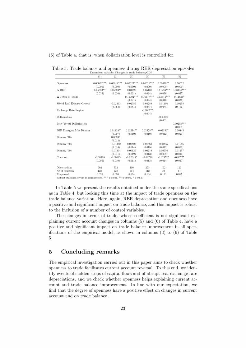
Table 5: Trade balance and openness during RER depreciation episodesDependent variable: Changes in trade balance/GDP

(1) (2) (3) (4) (5) (6)

Openness 0.00020*** 0.00018*** 0.00022*** 0.00021*** 0.00029** 0.00032(0.000) (0.000) (0.000) (0.000) (0.000) (0.000)

∆ RER 0.05333** 0.05393** 0.04026 0.05181 0.11216*** 0.08134***(0.023) (0.026) (0.031) (0.034) (0.026) (0.027)

∆ Terms of Trade 0.16002*** 0.16477*** 0.13644*** 0.14633*(0.041) (0.044) (0.046) (0.079)

World Real Exports Growth -0.02353 0.02386 0.03289 0.01100 0.10255(0.064) (0.084) (0.087) (0.085) (0.122)

Exchange Rate Regime -0.00677*(0.004)

Dollarization -0.00084(0.001)

Levy Yeyati Dollarization 0.00203***(0.001)

IMF Emerging Mkt Dummy 0.01418** 0.02214** 0.02358** 0.02150* 0.00843(0.007) (0.010) (0.010) (0.012) (0.023)

Dummy ’70s 0.00933(0.013)

Dummy ’80s -0.01342 0.00825 0.01460 -0.01857 0.01056(0.014) (0.014) (0.015) (0.012) (0.022)

Dummy ’90s -0.01334 0.00136 0.00719 0.00750 0.01257(0.011) (0.012) (0.013) (0.009) (0.015)

Constant -0.00368 -0.00693 -0.02045* -0.00730 -0.02352* -0.03775(0.006) (0.010) (0.011) (0.013) (0.014) (0.037)



In Table 5 we present the results obtained under the same specificationsas in Table 4, but looking this time at the impact of trade openness on thetrade balance variation. Here, again, RER depreciation and openness havea positive and significant impact on trade balance, and this impact is robustto the inclusion of a number of control variables.

The changes in terms of trade, whose coefficient is not significant ex-plaining current account changes in columns (5) and (6) of Table 4, have apositive and significant impact on trade balance improvement in all spec-ifications of the empirical model, as shown in columns (3) to (6) of Table5

5 Concluding remarks

The empirical investigation carried out in this paper aims to check whetheropenness to trade facilitates current account reversal. To this end, we iden-tify events of sudden stops of capital flows and of abrupt real exchange ratedepreciations, and we check whether openness helps explaining current ac-count and trade balance improvement. In line with our expectation, wefind that the degree of openness have a positive effect on changes in currentaccount and on trade balance.

23

Our results indicate that more open economies can rebalance their cur-rent account and trade balance with smaller domestic currency devaluationsafter an external shock, such as sudden stop or currency crisis. Hence, moreopen economies would be better able to surpass external shocks that entailsthe need of current account reversals.

We present a theoretical framework that presents the mechanism throughwhich openness should affect the relation between current account changesand real exchange depreciation. Notice that, according to our simple frame-work, the size of the RER depreciation has not impact on welfare. Welfarechanges depend on the size of the income shocks that cause the suddenstop, but not on how the economy adapts to it. More specifically, if itadjust through major relative price changes or through income effects.

References

Alesina, A. and A. F. Wagner (2006, 06). Choosing (and reneging on) ex-change rate regimes. Journal of the European Economic Association 4 (4),770–799.

Bianchi, J. (2011, September). Overborrowing and systemic externalities inthe business cycle. American Economic Review 101 (7), 3400–3426.

Calderon, C. and M. Kubota (2013). Sudden stops: Are global and localinvestors alike? Journal of International Economics 89 (1), 122 – 142.

Calvo, G. A., A. Izquierdo, and L.-F. Mejia (2004). On the empirics ofsudden stops: The relevance of balance-sheet effects. NBER WorkingPapers 10520, National Bureau of Economic Research, Inc.

Cavallo, E. A. and J. A. Frankel (2008). Does openness to trade make coun-tries more vulnerable to sudden stops, or less? using gravity to establishcausality. Journal of International Money and Finance 27 (8), 1430 –1452.

Edwards, S. (2004). Financial openness, sudden stops, and current-accountreversals. The American Economic Review 94 (2), pp. 59–64.

Glick, R. and M. Hutchison (2011). Currency crises. Working Paper Series2011-22, Federal Reserve Bank of San Francisco.

Guidotti, P. E., F. Sturzenegger, A. Villar, J. d. Gregorio, and I. Gold-fajn (2004). On the consequences of sudden stops [with comments].Economıa 4 (2), pp. 171–214.

Korinek, A. and E. G. Mendoza (2013, August). From sudden stops tofisherian deflation: Quantitative theory and policy implications. WorkingPaper 19362, National Bureau of Economic Research.

24

Laeven, L. and F. Valencia (2012). Systemic banking crises database: Anupdate. IMF Working Papers 12/163, International Monetary Fund.

Mendoza, E. G. (2005). Real exchange rate volatility and the price of non-tradable goods in economies prone to sudden stops. Economia.

Milesi-Ferretti, G.-M. and A. Razin (2000, July). Current account reversalsand currency crises, empirical regularities. In Currency Crises, NBERChapters, pp. 285–326. National Bureau of Economic Research, Inc.

Reinhart, C. M. and K. S. Rogoff (2004). The modern history of exchangerate arrangements: A reinterpretation. The Quarterly Journal of Eco-nomics 119 (1), 1–48.

Rey, H. and P. Martin (2006). Globalization and emerging markets: Withor without crash? American Economic Review 96 (5), 1631–1651.

25

Documents

Current Account and Real Exchange Rate changes: the impact …€¦ · Current Account and Real Exchange Rate changes: the impact of Trade Openness Davide Romelli Universit e de Cergy-Pontoise,