Currency Substitution, Speculation, and Crises:

Theory and Empirical Analysis

by

Yasuyuki Sawada

Associate Professor, University of Tokyo

and

Pan A. Yotopoulos

Professor (em.) Stanford University and Professor, University of Florence

March 2002

Please address correspondence to: Professor Pan A. Yotopoulos FRI – Encina West # 314 Stanford University Stanford, CA 94305-6084 Phone: (650) 723-3129; Fax (650) 329-8159 E-mail: yotopoulos@stanford.edu

• We would like to thank Adrian Wood for helpful suggestions and for data support. We also would like to thank the members of Seminars and Workshops at the Economic and Social Research Institute of the Japanese Government’s Cabinet Office, Stanford University, the University of California, Berkeley, the University of Tokyo, the University of Siena, and personally, Alain de Janvry, Eiji Fujii, Koichi Hamada, Sung Jin Kang, Ryuzo Miyao, Kwanho Shin, Donato Romano, Hiroshi Shibuya, Shinji Takagi, Yosuke Takeda and Kazuo Yokokawa for useful comments on an earlier version of this paper. Needless to say, we are responsible for the remaining errors.

Currency Substitution, Speculation, and Crises:

Theory and Empirical Analysis

Abstract:

We extend the “fundamentals model” of currency crisis by incorporating the currency substitution effects

explicitly. In a regime of free foreign exchange markets and free capital movements the reserve (hard)

currencies are likely to substitute for the local soft currency in agents’ portfolia that include currency as an

asset. Our model shows that, controlling for the fundamentals of an economy, the more pronounced the

currency substitution is in a country, the earlier and the stronger is the tendency for the local currency to

devalue. The model is implemented by constructing a currency-softness index. Two empirical findings

emerge. First, there is a negative relationship between the currency-softness index and the degree of

nominal-exchange-rate devaluation. Second, there is a systematic negative relationship between the

softness of a currency and the level of economic development. The empirical and policy implications of

the model can prove germane in approaching "speculative attacks" on currencies and in evaluating

proposed dioramas of the “new architecture” of the international financial system.

JEL Classification: F31, F41, G15 Key words: Financial crises, incomplete markets, the new international financial order, currency substitution, free currency markets

2

Currency Substitution, Speculation, and Crises:

Theory and Empirical Analysis

1. Introduction

Money enters agents’ intertemporal budget constraint as an asset. A subset of money, currency,

is the monetary asset par excellence because of its liquidity characteristics. Moreover, when it is

transacted freely in an open economy, a country’s currency can be readily converted into internationally

tradable goods and into other currencies as well. Besides its attributes as a store of value and a medium of

exchange, the characteristics of liquidity and convertibility make currency into a super-asset that finds a

prominent place in agents’ portfolia. But not all currencies were created equal. From the point of view of

asset value currencies occupy a continuum from the reserve, to the hard, the soft, and the downright

worthless. Only reserve/ hard currencies are treated as store of value internationally, and they are held by

central banks in their reserves. This asset-value quality of a reserve currency is based on reputation,

which in the specific case means that there is a credible commitment to stability of reserve-currency prices

relative to some other prices that matter.1 Soft currencies, on the other hand, lack this implicit warrantee

of relative price stability.

A basic premise of this paper is that there is an ordinal preference-ranking for currencies that

becomes important when one uses a currency for asset-holding purposes. Moreover, in a free currency

market agents can implement this ranking by moving to higher-ranking monetary assets at small

transaction cost. In a free currency market where an agent has the choice of holding any currency as an

asset, why not hold the best currency there is – the reserve currency that Central Banks also hold in their

reserves? A free currency market, therefore, sets off a systematic process of currency substitution: the

1 Reputation in this context is different from credibility that entered the literature on foreign exchange management following the seminal article of Barro and Gordon (1983). In that literature reputation is related to time inconsistency when policy-makers renege on their commitment to target one of the two alternative targets, the inflation rate or the balance of payments. For examples of this literature see Agénor (1994) and references therein.

3

substitution of the reserve/hard currency for the soft.2 Currency substitution is the outcome of asymmetric

reputation between, e.g., the dollar and the peso in the positional continuum of currencies.3 It results in an

asymmetric demand from Mexicans to hold dollars as a store of value, a demand that is not reciprocated

by Americans holding pesos as a hedge against the devaluation of the dollar!4 This can lead to a

systematic instability in exchange rate parities. Girton and Roper (1981), for example, emphasized that

currency substitution can magnify small swings in expected money growth differentials into large changes

in exchange rates. Kareken and Wallace (1981) also showed that the free-market international economy

generates the multiplicity of equilibrium exchange rates which highlight the potential instabilities caused

by currency substitution. Our specific focus is the substitution of the hard currency for the soft and the

ensuing systematic devaluation of the latter. Capital flight constitutes a form of this currency substitution.

A complete flight from a currency, in the form of dollarization, represents the extreme case where any or

all of the three functions of a currency - unit of account, means of exchange, and, in particular, store of

value – are discharged in a foreign currency (Calvo and Végh, 1996).

We extend the “fundamentals model” (or the “first-generation model”) of currency crisis by

incorporating the endogenous currency substitution effects explicitly. Recently, several papers have tried

to extend this “first-generation model” by introducing an endogenous risk premium or an endogenous

regime-switching of economic policy (Flood and Marion, 2000; Cavallari and Corsetti, 2000). By

focusing on an optimal dynamic response of domestic agents our model is distinguished within this genre

2 Our definition of currency substitution is not the only one employed in the literature. In fact the concept of currency substitution is rather ambiguous in economics. For a survey of different definitions, see Giovannini and Turtelboom (1994). 3 In this formulation of the reputation-based continuum between reserve/hard and soft currencies, a free currency market makes foreign exchange into a “positional good” (Hirsch, 1976; Frank and Cook, 1976; Frank, 1985; Pagano, 1999). Following that literature, in a shared system of social status, e.g., it becomes possible for an individual (a good) to have a positive amount of prestige (reputation) such as a feeling of superiority, only because the other individuals (other goods) have a symmetrical feeling of inferiority, i.e., negative reputation (Pagano, 1999). In a free currency market, the simple fact that reserve currencies exist, implies that there are soft currencies that are shunned for some (asset-holding) purposes. 4 Keynes (1923) called “precautionary” this new slice added on the demand for foreign exchange that impinges asymmetrically on the conventional demand-and-supply model for determining exchange rate

4

of recent literature by its generality. We show that the more pronounced the currency substitution is in a

country the earlier and the stronger is the tendency for the local currency to devalue. This tendency holds

whether the origins of currency substitution lie in a risk premium or simply in a "taste" for ratcheting up

liquid asset holdings to a harder currency. The intuition behind our theory is straightforward. With strong

currency substitution arising from the concern about future devaluations the demand for the domestic

(soft) currency, relative to the foreign (hard) currency, declines. Given the stream of domestic money-

supply growth, a decline in domestic money demand will increase the equilibrium domestic price level.

This increased domestic price level will lead to devaluation of the nominal exchange rate. A novel feature

of this paper is to show empirically that, controlling for the fundamentals, the reputation-asymmetry via-a-

vis the reserve currencies triggers systematic devaluations of the soft currencies of emerging economies

and developing countries.5

The paper is organized as follows. Section 2 sets the main thrust of this paper in the context of the

literature. Section 3 extends the fundamentals model of the currency crisis by incorporating the currency

substitution effect. The empirical model and results are presented in Section 4. Section 5 presents the

policy implications of the currency substitution hypothesis of devaluation, emphasizing specifically the

departures from the conventional treatment of financial crises. It turns out, for example, that the simple

extension of incorporating in the extant models currency substitution becomes germane for modeling

"speculative attacks" on a currency and for designing the "new architecture" of the international financial

system. The concluding Section 6 follows.

2. The Predecessors

This paper builds on two strands of the literature. Krugman (1979) first developed a model of the

balance of payment crisis due to speculative attacks on the fixed-exchange-rate regime. Flood and Garber

parity. 5 In a two-country general equilibrium model one could show the impact of asymmetric reputation as a zero-sum game (Pagano, 1999). For simplicity, we consider only one-sided reputation in this paper.

5

(1984) presented the linear version of Krugman’s model. This crop of the “first generation” models

fingers the deteriorating “fundamentals ” of an economy as the trigger to the currency crisis (Eichengreen,

Rose, and Wyplosz, 1994).

It seems that this literature implicitly assumes that the important role of money is as a medium of

exchange, since the model introduces the arbitrage equation of tradable goods prices or the purchasing

power parity equation. The idea of money as the medium of exchange was expanded in two alternative

directions that formalized the micro-foundation of the money demand function: the cash-in-advance

model (Clower, 1967; Lucas and Stokey, 1987) and the transaction model (Baumol, 1952; Tobin, 1956).

In either model, money is held for transaction purposes. However, money also serves as a store of value,

and enters as such the utility function. Sidrauski (1967) first formulated the Ramsey optimal growth

model with both consumption and real money balances in the utility function subject to an intertemporal

budget constraint with money.

From the technical perspective, in order to examine whether putting money in the utility function

is appropriate, we can ask whether it is possible to rewrite the maximization problem of an agent with

transaction costs of money holdings. Feenstra (1986) showed that maximization subject to a Baumol-

Tobin transaction technology can be approximately rewritten as maximization with money in the utility

function. Moreover, the simple cash-in-advance model of money can be written as a maximization

problem by ignoring the cash-in-advance constraint but introducing money in the utility function

(Blanchard and Fischer, 1989: 192). Also Obstfeld and Rogoff (1996: 530-532) showed that the money-

in-utility-function formula can be viewed as a derived utility function that includes real balances because

agents economize on time spent in transacting. Therefore, the-money-in-utility-function formula can be

regarded as a general formulation of the micro-foundations of the money demand function.

The novelty in our model lies in fusing and expanding both strands of this literature into a micro-

fundamentals model in which optimizing agents engage in currency substitution thus setting-off

endogenously serial devaluations that can culminate in a currency crisis. In the process, we expand

Krugman's model by introducing money not only as a medium of exchange but also in its role as an asset.

6

Moreover, the utility function in our model contains both domestic and foreign currency, with possibilities

of substituting one for the other, especially for asset-holding purposes. Flood and Marion (2000) and

Cavallari and Corsetti (2000) extended the first-generation model of currency crises by incorporating an

endogenous risk premium and by introducing an endogenous policy, respectively. Our contribution lies in

constructing and testing a general model that extends the first-generation model by introducing

endogenous currency substitution by optimizing agents.

3. The Fundamentals Model of Balance-of-Payments Crisis under Currency Substitution

If a country with a soft currency fixed its exchange rate initially, an expansionary fiscal and/or

monetary policy will render the fixed exchange rate regime untenable, sooner or later. In this section, we

will construct a simple model of currency crisis that is triggered by currency substitution. The model

portrays a situation where speculation-led crises can occur in a completely rational environment under the

basic principles of efficient asset-price arbitrage.

In what follows we first derive the optimal condition of currency substitution in a dynamic model

of optimizing agents. Then we extend the Obstfeld and Rogoff (1996) log-linear version of Krugman’s

(1979) model by introducing currency substitution effects while controlling for the fundamentals.

3.1 The Micro-fundamentals of Currency Substitution

Our focus is to model the role of money as an asset and a store of value. However in the real

world, money as a store of value is dominated by several assets. To account for this we construct a

dynamic optimization model of currency substitution, applying the basic setup of Obstfeld and Rogoff

(1996: 551-553). By definition, a domestic representative agent’s total money for asset-holding purposes,

M, is composed of domestic currency, M1 and foreign currency, MF:

Mt = M1t + εMFt

where ε is the nominal exchange rate. Then the optimal allocation of money-holding (of two different

7

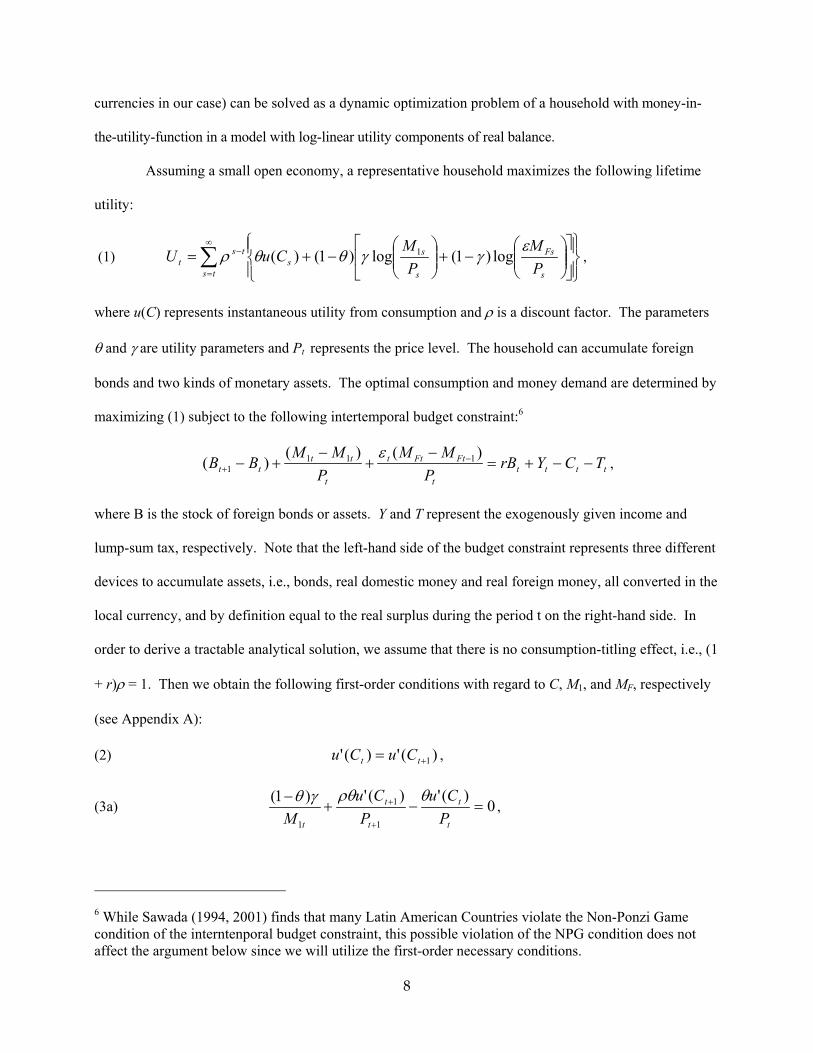
currencies in our case) can be solved as a dynamic optimization problem of a household with money-in-

the-utility-function in a model with log-linear utility components of real balance.

Assuming a small open economy, a representative household maximizes the following lifetime

utility:

(1)

−+

−+= ∑

∞

=

−

s

Fs

s

ss

ts

tst P

MP

MCu

εγγθθρ log)1(log)1()( 1U ,

where u(C) represents instantaneous utility from consumption and ρ is a discount factor. The parameters

θ and γ are utility parameters and Pt represents the price level. The household can accumulate foreign

bonds and two kinds of monetary assets. The optimal consumption and money demand are determined by

maximizing (1) subject to the following intertemporal budget constraint:6

ttttt

FtFtt

t

tttt TCYrB

PMM

PMM

BB −−+=−

+−

+− −+

)()()( 111

1ε

,

where B is the stock of foreign bonds or assets. Y and T represent the exogenously given income and

lump-sum tax, respectively. Note that the left-hand side of the budget constraint represents three different

devices to accumulate assets, i.e., bonds, real domestic money and real foreign money, all converted in the

local currency, and by definition equal to the real surplus during the period t on the right-hand side. In

order to derive a tractable analytical solution, we assume that there is no consumption-titling effect, i.e., (1

+ r)ρ = 1. Then we obtain the following first-order conditions with regard to C, M1, and MF, respectively

(see Appendix A):

(2) )(')(' 1+= tt CuCu ,

(3a) 0)(')(')1(

1

1

1

=−+−

+

+

t

t

t

t

t PCu

PCu

Mθρθγθ

,

6 While Sawada (1994, 2001) finds that many Latin American Countries violate the Non-Ponzi Game condition of the interntenporal budget constraint, this possible violation of the NPG condition does not affect the argument below since we will utilize the first-order necessary conditions.

8

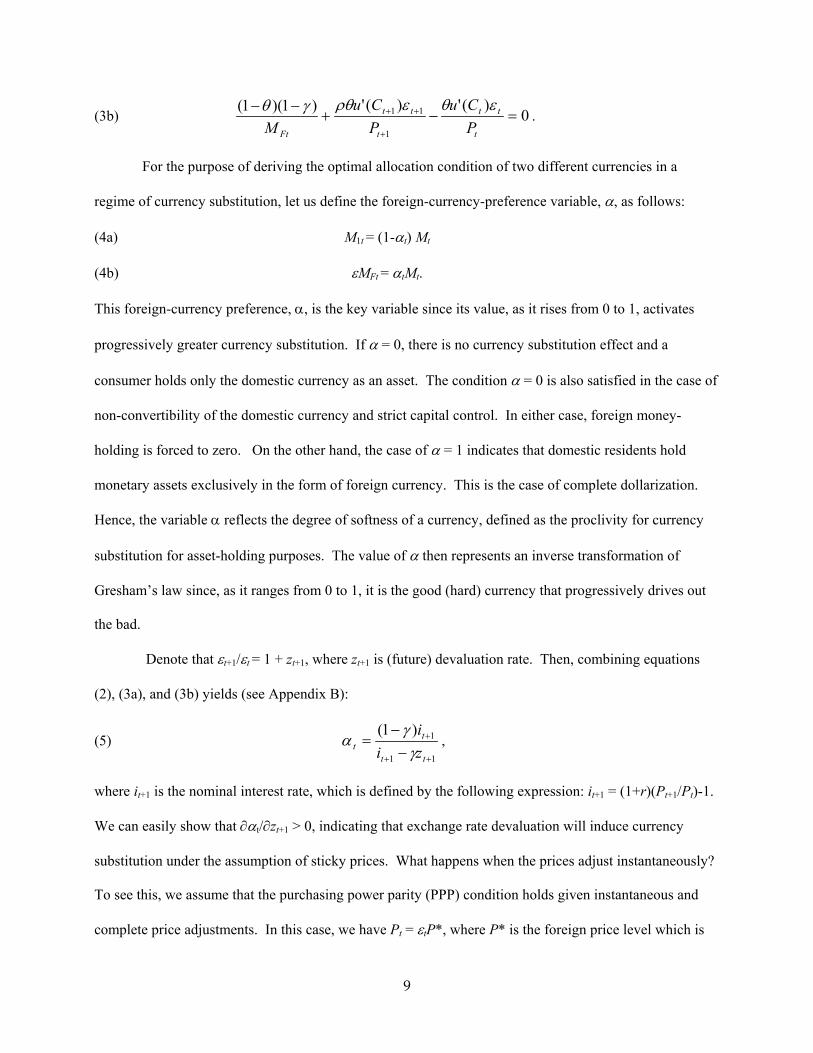
(3b) 0)(')(')1)(1(

1

11 =−+−−

+

++

t

tt

t

tt

Ft PCu

PCu

Mεθερθγθ

.

For the purpose of deriving the optimal allocation condition of two different currencies in a

regime of currency substitution, let us define the foreign-currency-preference variable, α, as follows:

(4a) M1t = (1-αt) Mt

(4b) εMFt = αtMt.

This foreign-currency preference, α, is the key variable since its value, as it rises from 0 to 1, activates

progressively greater currency substitution. If α = 0, there is no currency substitution effect and a

consumer holds only the domestic currency as an asset. The condition α = 0 is also satisfied in the case of

non-convertibility of the domestic currency and strict capital control. In either case, foreign money-

holding is forced to zero. On the other hand, the case of α = 1 indicates that domestic residents hold

monetary assets exclusively in the form of foreign currency. This is the case of complete dollarization.

Hence, the variable α reflects the degree of softness of a currency, defined as the proclivity for currency

substitution for asset-holding purposes. The value of α then represents an inverse transformation of

Gresham’s law since, as it ranges from 0 to 1, it is the good (hard) currency that progressively drives out

the bad.

Denote that εt+1/εt = 1 + zt+1, where zt+1 is (future) devaluation rate. Then, combining equations

(2), (3a), and (3b) yields (see Appendix B):

(5) 11

1)1(

++

+

−−

=tt

tt zi

iγ

γα ,

where it+1 is the nominal interest rate, which is defined by the following expression: it+1 = (1+r)(Pt+1/Pt)-1.

We can easily show that ∂αt/∂zt+1 > 0, indicating that exchange rate devaluation will induce currency

substitution under the assumption of sticky prices. What happens when the prices adjust instantaneously?

To see this, we assume that the purchasing power parity (PPP) condition holds given instantaneous and

complete price adjustments. In this case, we have Pt = εtP*, where P* is the foreign price level which is

9

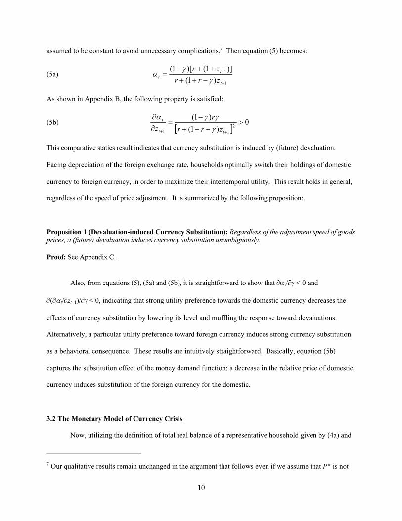
assumed to be constant to avoid unnecessary complications.7 Then equation (5) becomes:

(5a) 1

1

)1()]1()[1(

+

+

−++++−

=t

tt zrr

zrγ

γα

As shown in Appendix B, the following property is satisfied:

(5b) [ ]

0)1(

)1(2

11

>−++

−=

∂∂

++ tt

t

zrrr

z γγγα

This comparative statics result indicates that currency substitution is induced by (future) devaluation.

Facing depreciation of the foreign exchange rate, households optimally switch their holdings of domestic

currency to foreign currency, in order to maximize their intertemporal utility. This result holds in general,

regardless of the speed of price adjustment. It is summarized by the following proposition:.

Proposition 1 (Devaluation-induced Currency Substitution): Regardless of the adjustment speed of goods prices, a (future) devaluation induces currency substitution unambiguously. Proof: See Appendix C.

Also, from equations (5), (5a) and (5b), it is straightforward to show that ∂αt/∂γ < 0 and

∂(∂αt/∂zt+1)/∂γ < 0, indicating that strong utility preference towards the domestic currency decreases the

effects of currency substitution by lowering its level and muffling the response toward devaluations.

Alternatively, a particular utility preference toward foreign currency induces strong currency substitution

as a behavioral consequence. These results are intuitively straightforward. Basically, equation (5b)

captures the substitution effect of the money demand function: a decrease in the relative price of domestic

currency induces substitution of the foreign currency for the domestic.

3.2 The Monetary Model of Currency Crisis

Now, utilizing the definition of total real balance of a representative household given by (4a) and

7 Our qualitative results remain unchanged in the argument that follows even if we assume that P* is not

10

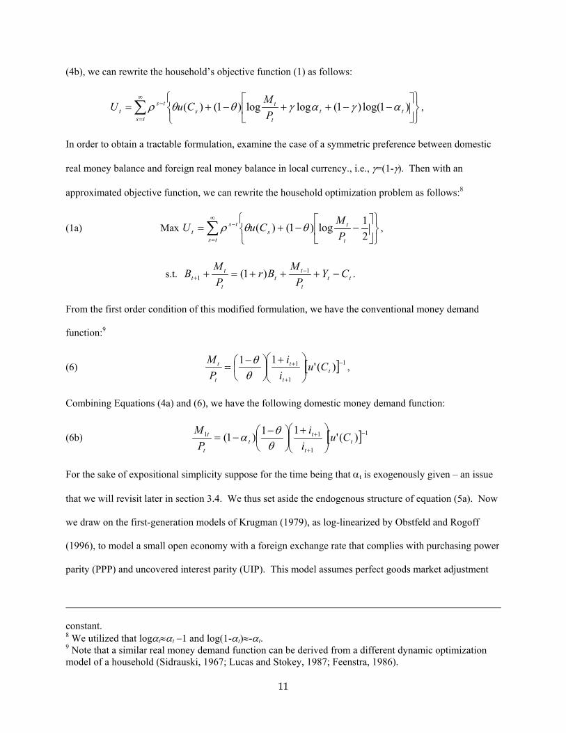
(4b), we can rewrite the household’s objective function (1) as follows:

−−++−+= ∑

∞

=

− )1log()1(loglog)1()( ttt

ts

ts

tst P

MCu αγαγθθρU ,

In order to obtain a tractable formulation, examine the case of a symmetric preference between domestic

real money balance and foreign real money balance in local currency., i.e., γ=(1-γ). Then with an

approximated objective function, we can rewrite the household optimization problem as follows:8

(1a) Max

−−+= ∑

∞

=

−

21log)1()(

t

ts

ts

tst P

MCu θθρU ,

s.t. ttt

tt

t

tt CY

PM

BrP

MB −+++=+ −

+1

1 )1( .

From the first order condition of this modified formulation, we have the conventional money demand

function:9

(6) [ ] 1

1

1 )('11 −

+

+

+

−

= tt

t

t

t Cui

iP

Mθ

θ,

Combining Equations (4a) and (6), we have the following domestic money demand function:

(6b) [ ] 1

1

11 )('11)1( −

+

+

+

−

−= tt

tt

t

t Cui

iP

Mθ

θα

For the sake of expositional simplicity suppose for the time being that αt is exogenously given – an issue

that we will revisit later in section 3.4. We thus set aside the endogenous structure of equation (5a). Now

we draw on the first-generation models of Krugman (1979), as log-linearized by Obstfeld and Rogoff

(1996), to model a small open economy with a foreign exchange rate that complies with purchasing power

parity (PPP) and uncovered interest parity (UIP). This model assumes perfect goods market adjustment

constant. 8 We utilized that logαt≈αt –1 and log(1-αt)≈-αt. 9 Note that a similar real money demand function can be derived from a different dynamic optimization model of a household (Sidrauski, 1967; Lucas and Stokey, 1987; Feenstra, 1986).

11

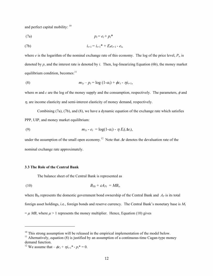
and perfect capital mobility: 10

(7a) pt = et + pt*

(7b) it+1 = it+1* + Etet+1 - et,

where e is the logarithm of the nominal exchange rate of this economy. The log of the price level, Pt, is

denoted by p, and the interest rate is denoted by i. Then, log-linearizing Equation (6b), the money market

equilibrium condition, becomes:11

(8) m1t – pt = log (1-αt) + φct - ηit+1,

where m and c are the log of the money supply and the consumption, respectively. The parameters, φ and

η, are income elasticity and semi-interest elasticity of money demand, respectively.

Combining (7a), (7b), and (8), we have a dynamic equation of the exchange rate which satisfies

PPP, UIP, and money market equilibrium:

(9) m1t - et = log(1-αt) - η Et(∆et),

under the assumption of the small open economy.12 Note that ∆e denotes the devaluation rate of the

nominal exchange rate approximately.

3.3 The Role of the Central Bank

The balance sheet of the Central Bank is represented as

(10) BHt + εAFt = MBt,

where BH represents the domestic government bond ownership of the Central Bank and AF is its total

foreign asset holdings, i.e., foreign bonds and reserve currency. The Central Bank’s monetary base is M1

= µ MB, where µ > 1 represents the money multiplier. Hence, Equation (10) gives

10 This strong assumption will be released in the empirical implementation of the model below. 11 Alternatively, equation (8) is justified by an assumption of a continuous-time Cagan-type money demand function. 12 We assume that – φct + ηit+1* - pt* = 0.

12

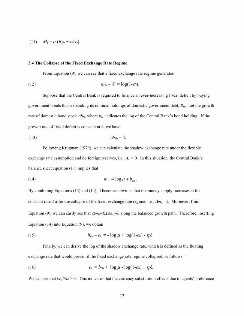
(11) M1 = µ (BHt + εAFt).

3.4 The Collapse of the Fixed Exchange Rate Regime

From Equation (9), we can see that a fixed exchange rate regime generates

(12) m1t – e = log(1-αt).

Suppose that the Central Bank is required to finance an ever-increasing fiscal deficit by buying

government bonds thus expanding its nominal holdings of domestic government debt, BH. Let the growth

rate of domestic bond stock ∆bH, where bH indicates the log of the Central Bank’s bond holding. If the

growth rate of fiscal deficit is constant at λ, we have

(13) ∆bH, = λ.

Following Krugman (1979), we can calculate the shadow exchange rate under the flexible

exchange rate assumption and no foreign reserves, i.e., AF = 0. In this situation, the Central Bank’s

balance sheet equation (11) implies that

(14) Htt bm += µlog1 .

By combining Equations (13) and (14), it becomes obvious that the money supply increases at the

constant rate λ after the collapse of the fixed exchange rate regime, i.e., ∆m1t=λ. Moreover, from

Equation (9), we can easily see that ∆m1t=Et(∆et)=λ along the balanced growth path. Therefore, inserting

Equation (14) into Equation (9), we obtain

(15) bHt – et = - log µ + log(1-αt) - ηλ

Finally, we can derive the log of the shadow exchange rate, which is defined as the floating

exchange rate that would prevail if the fixed exchange rate regime collapsed, as follows:

(16) et = bHt + log µ - log(1-αt) + ηλ.

We can see that ∂et /∂α > 0. This indicates that the currency substitution effects due to agents’ preference

13

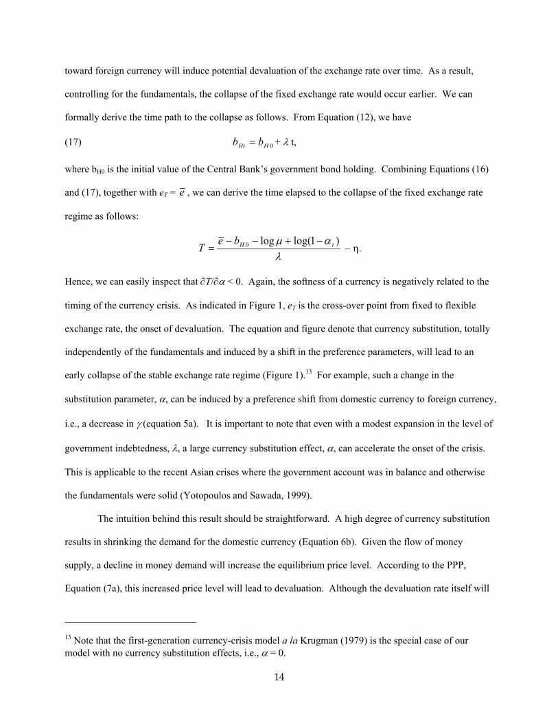
toward foreign currency will induce potential devaluation of the exchange rate over time. As a result,

controlling for the fundamentals, the collapse of the fixed exchange rate would occur earlier. We can

formally derive the time path to the collapse as follows. From Equation (12), we have

(17) b 0HHt b= + λ t,

where bH0 is the initial value of the Central Bank’s government bond holding. Combining Equations (16)

and (17), together with eT = e , we can derive the time elapsed to the collapse of the fixed exchange rate

regime as follows:

λαµ )1log(log0 tHbe

T−+−−

= − η.

Hence, we can easily inspect that ∂T/∂α < 0. Again, the softness of a currency is negatively related to the

timing of the currency crisis. As indicated in Figure 1, eT is the cross-over point from fixed to flexible

exchange rate, the onset of devaluation. The equation and figure denote that currency substitution, totally

independently of the fundamentals and induced by a shift in the preference parameters, will lead to an

early collapse of the stable exchange rate regime (Figure 1).13 For example, such a change in the

substitution parameter, α, can be induced by a preference shift from domestic currency to foreign currency,

i.e., a decrease in γ (equation 5a). It is important to note that even with a modest expansion in the level of

government indebtedness, λ, a large currency substitution effect, α, can accelerate the onset of the crisis.

This is applicable to the recent Asian crises where the government account was in balance and otherwise

the fundamentals were solid (Yotopoulos and Sawada, 1999).

The intuition behind this result should be straightforward. A high degree of currency substitution

results in shrinking the demand for the domestic currency (Equation 6b). Given the flow of money

supply, a decline in money demand will increase the equilibrium price level. According to the PPP,

Equation (7a), this increased price level will lead to devaluation. Although the devaluation rate itself will

13 Note that the first-generation currency-crisis model a la Krugman (1979) is the special case of our model with no currency substitution effects, i.e., α = 0.

14

be the growth rate of the money supply, it is the currency substitution that shifts the locus of the shadow

exchange rate toward the devaluation.

So far, for the sake of tractability, we have assumed that the currency substitution variable, α, is

exogenously given. Yet, equation (5b) and Proposition 1 indicate that this variable is endogenously

determined by a household’s dynamic optimization behavior. The true equilibrium exchange rate

behavior should take into account this endogeneity of the currency substitution variable. Although we

have imposed the perfect foresight assumption of the model so far, the future devaluation rate, zt+1 , should

be treated as an expected variable in reality. For convenience, we denote an expected devaluation rate as

zt+1e. A correct interpretation of Proposition 1 is that the foreign-currency-preference variable will

increase in response to an expected devaluation, i.e., αt = α (zt+1e) with ∂αt/∂zt+1

e>0, because of

endogeneity of the currency substitution variable, αt. Then once a country’s currency behaves as a soft

currency with an expected devaluation, the dynamic locus of the shadow exchange rate line, represented

by Equation (16), will shift toward further devaluation (Figure 1). In this case, even if a country is initially

at the point A’, where the speculative attacks are not profitable without currency substitution, a currency

substitution due to an expected devaluation can cause the immediate collapse of a fixed exchange rate

regime. Hence, the expectation of devaluation can become a self-fulfilling prophecy. Note that this story

does not depend on the usual assumption of the second generation model of currency crisis where the

existence of speculative bubbles itself generates multiple-equilibria and a self-fulfilling expectation of

speculative attacks (Obstfeld, 1996). Rather, in our model, the expectations of devaluation of optimizing

domestic residents make the collapse of the fixed exchange rate regime inevitable.

Moreover, as is often pointed theoretically and empirically, there is a habit-formation of currency

substitution (Uribe, 1997). The self-fulfilling expectation of devaluation is likely to have hysteresis on

currency substitution. This mechanism creates the possibility of self-validating devaluation spirals. An

expected devaluation generates currency substitution of agents [equation (5b)]. Currency substitution, in

turn, leads to a further expected devaluation [equation (16)]. Soft currencies depreciate systematically

15

because of the currency substitution effect and crises occur more frequently. This is a formal

representation of the Y-Proposition elaborated by Yotopoulos (1996, 1997).

4. Empirical Implementation

The previous sections have generalized the treatment of currency crises by introducing currency

substitution as a trigger for devaluation while controlling for the fundamentals of an economy. We can

examine this process intuitively by constructing an imperfect proxy of the currency substitution variable,

αt, and observing its behavior over time and especially during a crisis. Lacking data on foreign currency

deposits, we define the proxy as the ratio of time, savings, and foreign-currency deposits in the deposit

money banks to a broader measure of money, M2, which also includes time, savings, and foreign currency

deposits.14 Monthly data of these variables from January 1991 to September 2000 are extracted from

International Financial Statistics of the International Monetary Fund. This measure of currency

substitution can be regarded as the upper-bound of αt since the data commingle in the numerator foreign

currency deposits with other time and savings deposits.

Figure 2 represents the above ratio-proxy estimate of monthly currency substitution for Indonesia,

Korea, Malaysia, and Thailand. Over the period from January 1991 to September 2000, there was no

trend (except a slight upward trend in Indonesia) until July 1997 when there was a pronounced increase in

the proxy variable. Casual observation suggests a synchronicity between the increase in the proxy

variable and the currency devaluations of 1997 and 1998. This is consistent with our theoretical

framework: switching behavior from domestic to foreign currency ratchets up to devaluation. In Korea

particularly, gradual currency substitution preceded the massive devaluation of November 1997.

Actually, in our model currency substitution is no longer an issue of fundamentals. As long as

currency used for asset-holding purposes is a positional good and a free currency market provides for

currency switching at negligible transaction costs, it pays for agents to ratchet up by substituting the

14 Note that the deposit banks comprise commercial banks and other financial institutions that accept

16

reserve/ hard currency for the soft. Agents’ expectations for devaluation generate self-fulfilling outcomes.

Expectations thus become important determinants of devaluation.

4.1 The Empirical Model

The formal cross-country empirical implementation of the model rests on Equation (16) above

which represents a modified version of Krugman’s collapse of the fixed exchange rate regime, with eT

indicating the cross-over point from fixed to flexible exchange rate, denoting devaluation. The

modifications consist of introducing currency substitution that impacts on the timing of the collapse of the

exchange rate regime (Figure 1) and of releasing the strong assumption of perfect international capital

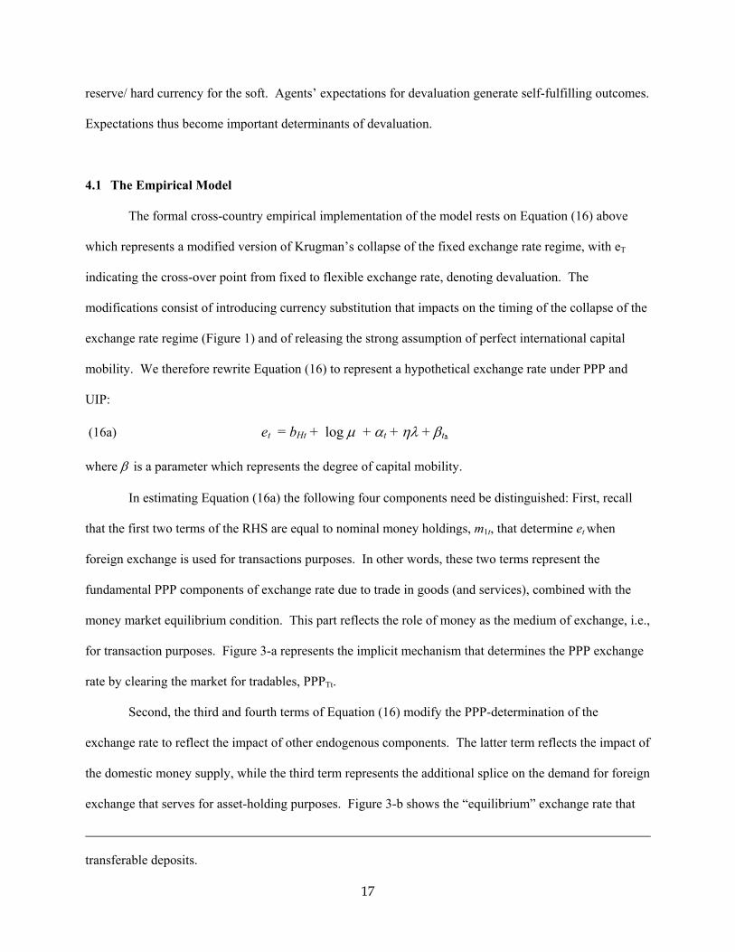
mobility. We therefore rewrite Equation (16) to represent a hypothetical exchange rate under PPP and

UIP:

(16a) et = bHt + log µ + αt + ηλ + βt,

where β is a parameter which represents the degree of capital mobility.

In estimating Equation (16a) the following four components need be distinguished: First, recall

that the first two terms of the RHS are equal to nominal money holdings, m1t, that determine et when

foreign exchange is used for transactions purposes. In other words, these two terms represent the

fundamental PPP components of exchange rate due to trade in goods (and services), combined with the

money market equilibrium condition. This part reflects the role of money as the medium of exchange, i.e.,

for transaction purposes. Figure 3-a represents the implicit mechanism that determines the PPP exchange

rate by clearing the market for tradables, PPPTt.

Second, the third and fourth terms of Equation (16) modify the PPP-determination of the

exchange rate to reflect the impact of other endogenous components. The latter term reflects the impact of

the domestic money supply, while the third term represents the additional splice on the demand for foreign

exchange that serves for asset-holding purposes. Figure 3-b shows the “equilibrium” exchange rate that

transferable deposits.

17

accounts also for currency substitution, α.

Third, the existence of effective capital control and rationing of the foreign exchange allocation is

captured bythe last term in Equation (16a) with β > 0 (Figure 3-c). In this case the “equilibrium”

exchange rate is overridden at a level higher than in Figure 3-b.15 The resulting foreign exchange rate is

the black market exchange rate, BM, which is higher than the equilibrium nominal exchange rate under

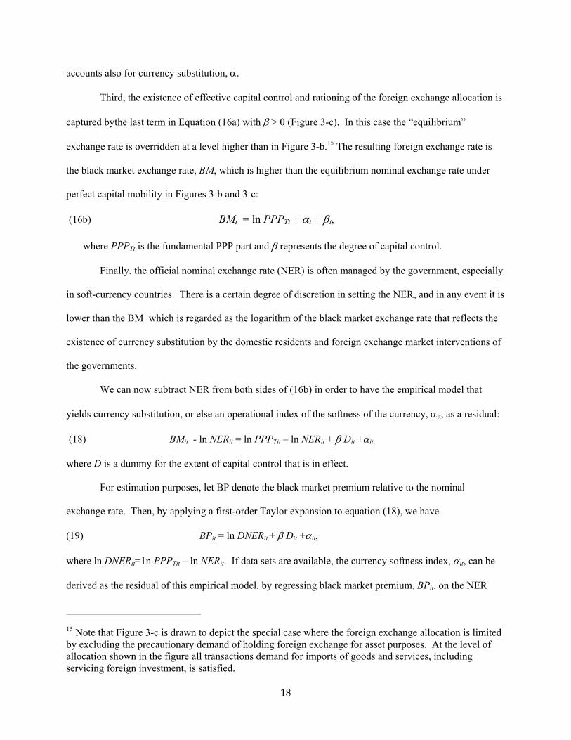
perfect capital mobility in Figures 3-b and 3-c:

(16b) BMt = ln PPPTt + αt + βt,

where PPPTt is the fundamental PPP part and β represents the degree of capital control.

Finally, the official nominal exchange rate (NER) is often managed by the government, especially

in soft-currency countries. There is a certain degree of discretion in setting the NER, and in any event it is

lower than the BM which is regarded as the logarithm of the black market exchange rate that reflects the

existence of currency substitution by the domestic residents and foreign exchange market interventions of

the governments.

We can now subtract NER from both sides of (16b) in order to have the empirical model that

yields currency substitution, or else an operational index of the softness of the currency, αit, as a residual:

(18) BMit - ln NERit = ln PPPTit – ln NERit + β Dit +αit,

where D is a dummy for the extent of capital control that is in effect.

For estimation purposes, let BP denote the black market premium relative to the nominal

exchange rate. Then, by applying a first-order Taylor expansion to equation (18), we have

(19) BPit = ln DNERit + β Dit +αit,

where ln DNERit=1n PPPTit – ln NERit. If data sets are available, the currency softness index, αit, can be

derived as the residual of this empirical model, by regressing black market premium, BPit, on the NER

15 Note that Figure 3-c is drawn to depict the special case where the foreign exchange allocation is limited by excluding the precautionary demand of holding foreign exchange for asset purposes. At the level of allocation shown in the figure all transactions demand for imports of goods and services, including servicing foreign investment, is satisfied.

18

distortion index, ln PPPTit – ln NERit, and the capital control indicator variable, Dit, which takes value of

one if there are any foreign exchange controls and zero otherwise.

Equation (19) calls for imposing coefficient restrictions. We thus estimate Equation (19) with

coefficient restriction on the NER distortion index, ln DNER, by using OLS with the Huber-White robust

standard error. Finally, we obtain the currency softness index, αit, as the estimated residuals of Equation

(19) with the coefficient restriction.16

4.2 The Data Set

In order to estimate the regression equation (19), we need three variables: the exchange-rate

black-market premium, BP; the nominal exchange rate, NER; the NER distortion index, 1n DNER; and

qualitative information about foreign capital controls.

First, the data for the black market premia on the foreign exchange rate are widely available from

different sources. We utilized a comprehensive annual cross-country panel data set of black market

premium, which is compiled by Adrian Wood (1999). This data set covers 42 countries over a period of

ten years (Table A2).

Second, consistent annual panel information on exchange rate restrictions is reported in Ernst &

Whinney (various years)17. The data denote restrictions on equity capital; debt capital; interest; dividends

and branch profits; and royalties, technical service fees, etc. Based on this information we construct a

binary variable of foreign capital control (Table A2).

Obtaining the appropriate NER distortion index that the theory requires is more difficult. The

empirical version of the NER distortion index that is broadly used for gauging a currency's tendency to

appreciate or depreciate is supposed to measure the deviation of the nominal exchange rate (NER) from

the ideal world where PPP holds and the prices of tradables tend to converge internationally (McKinnon,

1979). The empirical application of the index, however, whether it relies on the differential rate of

16 We also add time effects in this regression.

19

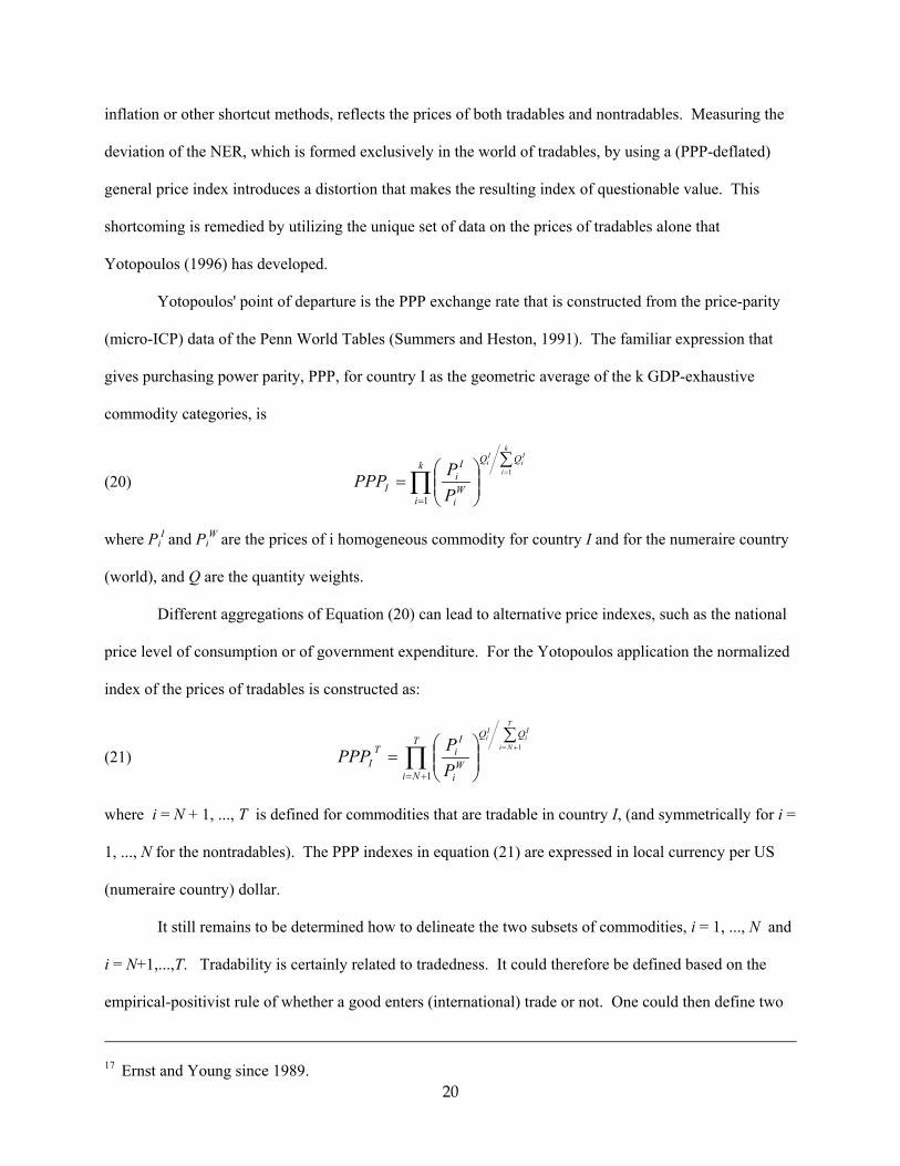
inflation or other shortcut methods, reflects the prices of both tradables and nontradables. Measuring the

deviation of the NER, which is formed exclusively in the world of tradables, by using a (PPP-deflated)

general price index introduces a distortion that makes the resulting index of questionable value. This

shortcoming is remedied by utilizing the unique set of data on the prices of tradables alone that

Yotopoulos (1996) has developed.

Yotopoulos' point of departure is the PPP exchange rate that is constructed from the price-parity

(micro-ICP) data of the Penn World Tables (Summers and Heston, 1991). The familiar expression that

gives purchasing power parity, PPP, for country I as the geometric average of the k GDP-exhaustive

commodity categories, is

(20) ∑

=

=

∏=

k

i

Ii

Ii QQk

iW

i

Ii

I PP

PPP1

1

where PiI and Pi

W are the prices of i homogeneous commodity for country I and for the numeraire country

(world), and Q are the quantity weights.

Different aggregations of Equation (20) can lead to alternative price indexes, such as the national

price level of consumption or of government expenditure. For the Yotopoulos application the normalized

index of the prices of tradables is constructed as:

(21) ∑

=

+=

∏+=

T

Ni

Ii

Ii QQT

NiW

i

IiT

I PP

PPP1

1

where i = N + 1, ..., T is defined for commodities that are tradable in country I, (and symmetrically for i =

1, ..., N for the nontradables). The PPP indexes in equation (21) are expressed in local currency per US

(numeraire country) dollar.

It still remains to be determined how to delineate the two subsets of commodities, i = 1, ..., N and

i = N+1,...,T. Tradability is certainly related to tradedness. It could therefore be defined based on the

empirical-positivist rule of whether a good enters (international) trade or not. One could then define two

20

17 Ernst and Young since 1989.

mutually exclusive categories of traded and nontraded goods. This heuristic approach, however, fails to

address some important issues. Is any participation in international trade sufficient to make a good

tradable? If so few nontradable goods would probably remain. Empirically Yotopoulos (1996: 112)

addresses the issue by adopting the standard definition of openness in an economy (the ratio of imports

and exports to GDP) and designating as tradable any commodity group that has exports plus imports

valued at more than 20 percent of the total share of that commodity’s expenditure in GDP. By

distinguishing a large number of commodity groups and by weighting both prices and the participation of

each individual commodity into tradability by actual expenditure weights, the arbitrariness of the criterion

has been blunted.

Implementation of the definition of the real exchange rate (RER) relies on the micro-PPP data of

the ICP (Kravis, Heston, and Summers, 1982; Penn World Tables). For the "basic classification" prices

and nominal and real per capita expenditures (expressed in domestic currency per U.S. dollar) are

available for 152 GDP-exhausting commodities for the "benchmark" countries and years. They were used

in a flexible aggregation form to derive prices of tradables and nontradables. The data for the definition of

tradability come from the United Nations Yearbook of International Trade Statistics which provides in 5-

digit SITC classification for each country the value of exports (f.o.b.) and imports (c.i.f.) in U.S. dollars.

The 5-digit classification was re-aggregated to achieve concordance with the ICP data. We constructed

the value of the index for tradable goods prices by using the data for the phases II, III, IV, and V of the

ICP for 1970, 1975, 1980, and 1985, respectively.

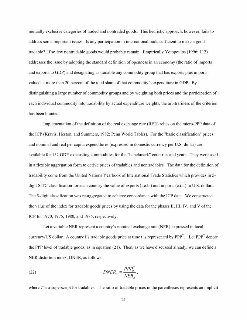
Let a variable NER represent a country’s nominal exchange rate (NER) expressed in local

currency/US dollar. A country i’s tradable goods price at time t is represented by PPPTit. Let PPPT denote

the PPP level of tradable goods, as in equation (21). Then, as we have discussed already, we can define a

NER distortion index, DNER, as follows:

(22) ,it

Tit

it NERPPP

DNER ≡

where T is a superscript for tradables. The ratio of tradable prices in the parentheses represents an implicit

21

long-run equilibrium purchasing power parity of tradable prices. Therefore, DNERit represents the

nominal exchange rate distortion, which is defined as the deviation of NER from the PPP for tradable

goods, i.e., the long-run equilibrium exchange rate. We can then formulate formally:

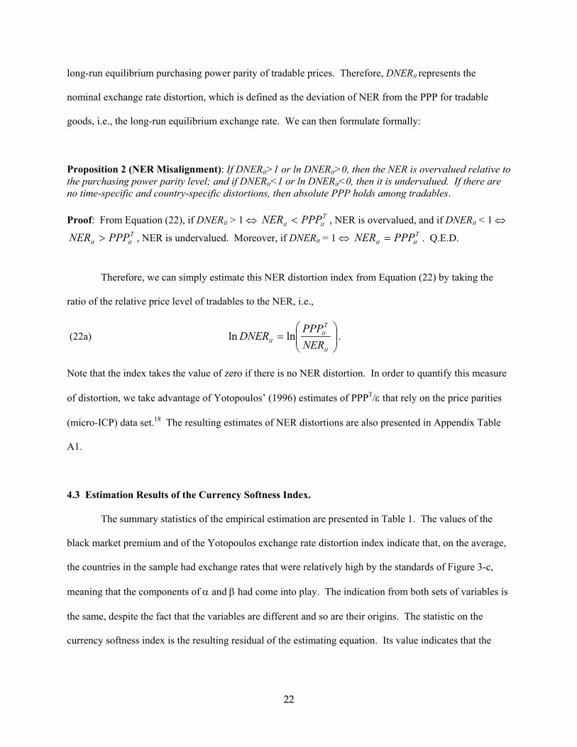
Proposition 2 (NER Misalignment): If DNERit>1 or ln DNERit>0, then the NER is overvalued relative to the purchasing power parity level; and if DNERit<1 or ln DNERit<0, then it is undervalued. If there are no time-specific and country-specific distortions, then absolute PPP holds among tradables. Proof: From Equation (22), if DNERit > 1 ⇔ , NER is overvalued, and if DNERT

itit PPPNER < it < 1 ⇔

, NER is undervalued. Moreover, if DNERTitit PPPNER > it = 1 ⇔ . Q.E.D. T

itit PPPNER =

Therefore, we can simply estimate this NER distortion index from Equation (22) by taking the

ratio of the relative price level of tradables to the NER, i.e.,

(22a)

=

it

Tit

it NERPPP

DNER lnln .

Note that the index takes the value of zero if there is no NER distortion. In order to quantify this measure

of distortion, we take advantage of Yotopoulos’ (1996) estimates of PPPT/ε that rely on the price parities

(micro-ICP) data set.18 The resulting estimates of NER distortions are also presented in Appendix Table

A1.

4.3 Estimation Results of the Currency Softness Index.

The summary statistics of the empirical estimation are presented in Table 1. The values of the

black market premium and of the Yotopoulos exchange rate distortion index indicate that, on the average,

the countries in the sample had exchange rates that were relatively high by the standards of Figure 3-c,

meaning that the components of α and β had come into play. The indication from both sets of variables is

the same, despite the fact that the variables are different and so are their origins. The statistic on the

currency softness index is the resulting residual of the estimating equation. Its value indicates that the

22

sample of countries, on the average, had soft currencies. This is consistent with the other statistics

described in the table.

As we can see, the exchange control has a positive and significant coefficient. This is consistent

with the theoretical prediction that foreign capital controls will increase a country’s foreign exchange

black market premium (Figure 3-c). Another finding is that the dummy for 1985 has a positive and

significant coefficient. This year-specific positive effect probably represents the impact of the significant

appreciation of US dollar in the early 1980s and the resultant systematic depreciation of other countries’

currencies toward the US dollar.

The immediate objective of Equation (19) is the derivation of the currency softness index, the

values of which are summarized in Table A2. This statistic, besides revealing important country- and

time-specific information, could also be used for investigating causality in various episodes of currency

crisis. Unfortunately the data set and the episodes of currency crises are not rich enough to rigorously

investigate causality hypotheses. However, we can still examine empirically the relevance of the currency

softness index to financial crises by other methods. In order to characterize empirically the currency

softness, we employ two different approaches.

First, the relationship between the softness measure and the currency distortion index is

represented in Figure 4. The Figure clearly indicates a negative relationship between the constructed

currency softness index and the degree of NER overvaluation. The fact that soft currencies are more

likely to be undervalued (i.e., too many pesos to the dollar) is consistent with the theoretical expectation of

the model. The operational difference between a hard and soft currency is that the exchange rate for the

latter reflects not only the demand and supply of foreign exchange for transaction (balance-of-payments)

purposes, but includes also an additional splice of “precautionary” demand for foreign exchange to be held

as an asset. This additional demand for hard currency will lead to devaluation of the exchange rate for the

soft currency as long as the hard-currency-country residents do not need to hedge their domestic-money-

18 The resulting estimates of NER distortions are available from the authors upon request.

23

asset holdings by accumulating soft currency. The asymmetry in demand for the “other” currency for

asset-holding purposes is rooted in asymmetric reputation between the reserve/hard and the soft currency

in free currency markets. It is precisely this asymmetry that characterizes serial devaluations and financial

crises as predominantly soft-currency phenomena. The tendency then for soft currencies to have “high”

nominal exchange rates in Equation (22) drives the DNER values below 1 (and to negative territory) thus

indicating a perennially undervalued domestic currency. This is consistent with the findings of

Yotopoulos (1996: Chapter 6) in the original study of exchange rate parity relying on micro-PPP data.

Also, we can easily see that capital control is negatively related with the currency substitution/softness

indicator, α, which is fully consistent with our theoretical framework in Section 2.1. Controls imposed on

domestic agents engaging in capital flight, on the other hand, tend to moderate the degree of the currency

substitution, and therefore of the undervaluation of the soft currency.

The second empirical finding relates to the negative relationship between the currency softness

index and per capita real GDP as is verified in Figure 5.19 To examine this relationship statistically, we

regressed the estimated currency softness index on the per capita GDP. We also included the year dummy

variables in order to control for a potential bias due to year-specific systematic effects. The estimation

results are presented in Table 3. The coefficient of per capita GDP is negative and highly significant.

This result confirms that there is a systematic relationship between the credibility of a currency and the

level of economic development. This argument is consistent with the story that a less-developed country

is more likely to be subjected to systematic devaluations due to its reputation-challenged currency. In

fact, there might be a circular causation between a currency's softness and a country’s low level of

economic development. Unconstrained by controls, residents in a poor economy prefer holding the dollar

because the domestic currency lacks in its credibility. A poor country, in turn, finds it difficult to establish

its currency’s reputation because of the low level of economic development. This two-way causality

could conceivable turn into a poverty trap for a country at a low stage of economic development.

19 Data on per capita real GDP is extracted from Summers and Heston (1991) Penn World Tables.

24

The obverse side of this finding holds that the best way for a soft currency to acquire reputation

and therefore to act with impunity like a hard currency, e.g., by removing all controls, is for development

to succeed. In other words, liberalizing the currency market as a policy (dis)intervention for promoting

development amounts to putting the cart in front of the horse. A currency cannot become hard by

behaving like a hard currency, i.e., by trading freely in the world’s exchange markets. There is an

appropriate sequence in the process of economic liberalization. Freeing the foreign exchange market

comes towards the end of this process when the main business of development has been done

(Yotopoulos, 1996: Chapter 11).

5. Speculative Attacks and Policy Implications

The first-generation models of financial crises have focused on balance-of-payments disequilibria

and the collapse of the fundamentals of an economy. Our model, on the other hand, predicts that even

under a prudent fiscal policy and with pristine economic fundamentals, strong currency substitution

precipitates a devaluation that may turn into a financial crisis. The analytical distinction between the two

approaches lies in the economic function of money that has been incorporated in each. By focusing on the

balance of payments, the extant models of financial crises consider the function of money as a medium of

exchange in the (international) market for goods and services. The currency substitution hypothesis

considers also the role of money as a store of value. While all currencies can do service, better or worse,

for transaction purposes, when used as store of value they are ranked in a definite pecking order from the

reserve/hard, to the soft, and to the worthless currency in a decreasing order of usefulness. There is a

positional continuum in holding currency as an asset based on its reputation. Reputation in this specific

case means that there is a credible commitment to stability of currency prices relative to some other prices

that matter – and this commitment is more credible, the closer a currency is to the reserve currency. Their

inherent asset value places reserve currencies in central banks’ reserves, and also makes them safe havens

for international capital movements. By the same token, the demand for foreign exchange – and

especially for reserve and hard currencies - becomes an important component in a representative agent’s

25

utility function regardless of the motivation for holding such assets, whether it is for portfolio

diversification, speculation or hedging.

The underlying asymmetry in reputation between soft and hard currency implies a corresponding

asymmetry in the determination of their respective exchange parities in a free currency market. While

transactions demand for foreign exchange is the principal determining factor of the price of both hard and

soft currencies, in the case of the latter the demand for foreign exchange for asset-holding purposes plays

an important role in decreasing the price of the currency (devaluation) and in exacerbating exchange rate

instability. Asymmetrically, the same demand by a soft-currency country drives the price of the hard

currency to appreciation – and appreciation, if it becomes problematic, is easier to combat than

depreciation. Soft currencies, as a result, are likely to be more “undervalued” (and more difficult to

remedy) than hard currencies that may tend to become “overvalued.” Herein lies the emblematic

difference between the currency substitution hypothesis and the extant interpretations of currency crises.

In the mainstream view devaluation always retains its salutary healing effects by matching supply and

demand and storing up the current account, thus eventually improving the fundamentals. In the currency

substitution alternative, on the other hand, devaluation will increase the value of the parameter

∂αt/∂zt+1e>0 (in Section 3.4) thus leading to an increased demand of foreign exchange for asset holding

purposes. In this view, competitive price-setting of foreign exchange for a soft currency represents “bad

competition” and can lead to “a race for the bottom,” i.e., to further serial devaluations. It becomes

intuitively clear that this interpretation of the foreign exchange market for a soft currency amounts to a

market incompleteness because of asymmetric reputation. This case corresponds fully to the parallel

literature of incomplete credit markets for reasons of asymmetric information (Stiglitz and Weiss, 1981).

The empirical implications of the two types of market incompleteness are also concordant. The policy

implication of rationing foreign exchange and imposing a mildly repressed exchange rate replicates the

need for credit controls for circumventing the “bad competition” and the “race for the bottom” that

competitive price-setting implies for the credit market. Capital controls become expedient in the case of

26

an incomplete foreign exchange market only to the extent that the inflow of financial capital contributes to

fanning (cheap) currency substitution of the soft local currency. Otherwise, there is no need for imposing

restrictions on direct foreign investment inflows or on outflows for the purpose of settling current account

imbalances, or of repatriation of capital and profits (Yotopoulos, 1996, 1997; Yotopoulos and Sawada,

1999).

The case of speculative attacks on a currency, as made in the literature, is related to financial

capital flows in the form of “hot money.” This is a special case of the currency-substitution-induced

devaluation in the model where unregulated inflows of financial capital can increase the value of the

parameter αt. In a free currency market, where devaluation may happen, or it may not, the holder of the

soft currency is offered a one-way-option: by substituting the hard currency for the soft, there is a capital

gain to be reaped if devaluation happens, while there is not an equivalent loss if it does not. This one-way

bet is also offered to the “speculator” who can sell short the soft currency. It is especially attractive to

foreign fund managers who can borrow the soft currency locally by leveraging a few million dollars’

deposit into a peso loan with the proceeds, in turn, converted into dollars. This play of draining the

Central Bank’s reserves makes the devaluation of the peso a self-fulfilling prophecy. And when

devaluation comes, the international investor can pay back the loan in cents on the dollar and take his hot

money across the Rio Grande.20 The entire process is initiated by taking advantage of the free currency

market to convert a soft-currency monetary asset into hard currency, thus asymmetrically increasing the

asset-demand for the latter and leading to the depreciation of the former.

The testable implication of this view of the role that financial capital can play in devaluations and

financial crises relates to the timing of capital outflow. The currency substitution hypothesis would

20 A variant of this approach, fine-tuned for the existence of a Monetary Board, was used by fund managers in Hong Kong in September 1998. By selling short the Hang Seng stock market index and at the same time converting HK dollars into US dollars they helped deplete the Monetary Board’s reserves thus forcing a monetary contraction. The increase in interest rates that followed fuelled a shift in assets from stocks to bonds, and a sharp decline in the stock market that rewarded the speculators with profits on their shorts. The scheme came to an abrupt end when the Hong Kong authorities intervened in support of the stock market (Yotopoulos and Sawada, 1999).

27

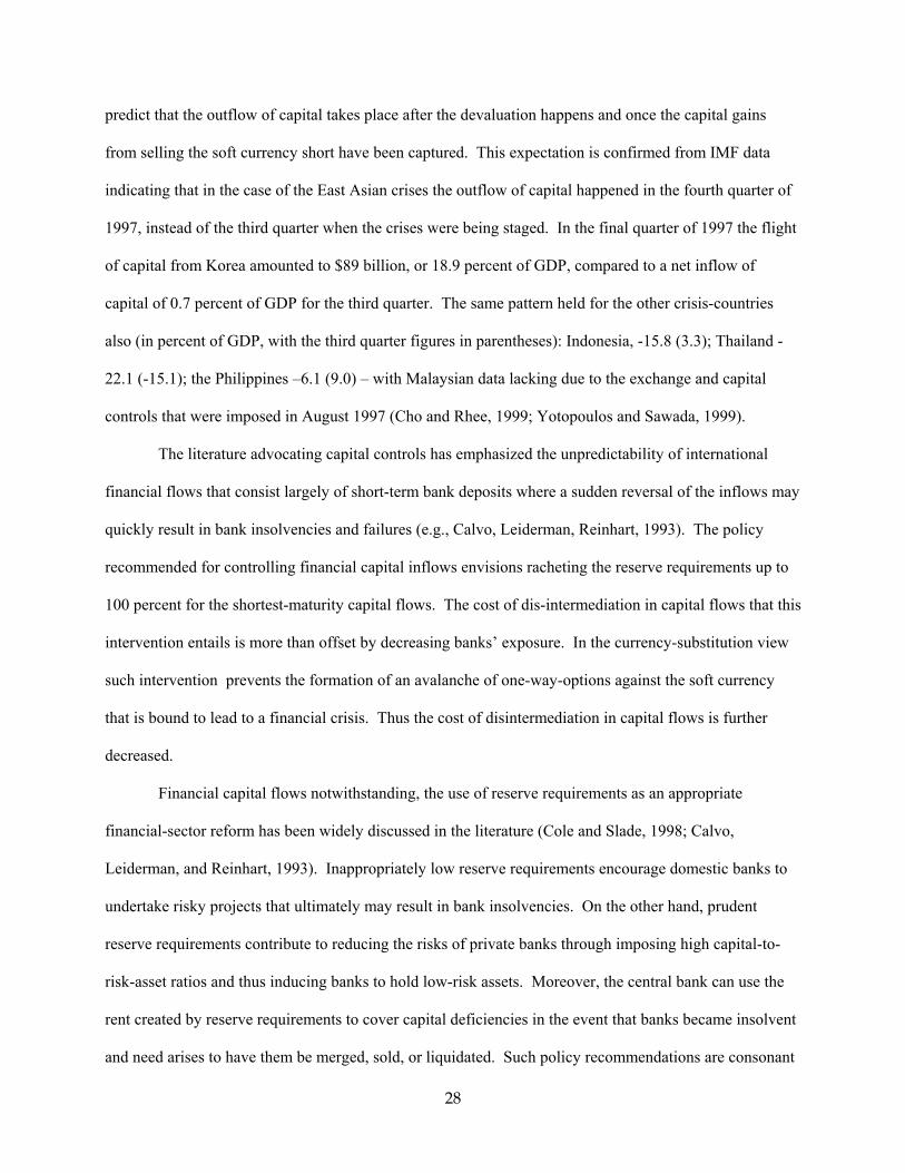
predict that the outflow of capital takes place after the devaluation happens and once the capital gains

from selling the soft currency short have been captured. This expectation is confirmed from IMF data

indicating that in the case of the East Asian crises the outflow of capital happened in the fourth quarter of

1997, instead of the third quarter when the crises were being staged. In the final quarter of 1997 the flight

of capital from Korea amounted to $89 billion, or 18.9 percent of GDP, compared to a net inflow of

capital of 0.7 percent of GDP for the third quarter. The same pattern held for the other crisis-countries

also (in percent of GDP, with the third quarter figures in parentheses): Indonesia, -15.8 (3.3); Thailand -

22.1 (-15.1); the Philippines –6.1 (9.0) – with Malaysian data lacking due to the exchange and capital

controls that were imposed in August 1997 (Cho and Rhee, 1999; Yotopoulos and Sawada, 1999).

The literature advocating capital controls has emphasized the unpredictability of international

financial flows that consist largely of short-term bank deposits where a sudden reversal of the inflows may

quickly result in bank insolvencies and failures (e.g., Calvo, Leiderman, Reinhart, 1993). The policy

recommended for controlling financial capital inflows envisions racheting the reserve requirements up to

100 percent for the shortest-maturity capital flows. The cost of dis-intermediation in capital flows that this

intervention entails is more than offset by decreasing banks’ exposure. In the currency-substitution view

such intervention prevents the formation of an avalanche of one-way-options against the soft currency

that is bound to lead to a financial crisis. Thus the cost of disintermediation in capital flows is further

decreased.

Financial capital flows notwithstanding, the use of reserve requirements as an appropriate

financial-sector reform has been widely discussed in the literature (Cole and Slade, 1998; Calvo,

Leiderman, and Reinhart, 1993). Inappropriately low reserve requirements encourage domestic banks to

undertake risky projects that ultimately may result in bank insolvencies. On the other hand, prudent

reserve requirements contribute to reducing the risks of private banks through imposing high capital-to-

risk-asset ratios and thus inducing banks to hold low-risk assets. Moreover, the central bank can use the

rent created by reserve requirements to cover capital deficiencies in the event that banks became insolvent

and need arises to have them be merged, sold, or liquidated. Such policy recommendations are consonant

28

with the model of currency substitution that champions a conservative fiscal and monetary policy for

avoiding a currency-substitution-led devaluation. To verify the importance of this intervention note that a

lower money multiplier will put off the timing of the collapse of the fixed exchange rate regime since

∂T/∂µ < 0. Recall that the money multiplier is defined as µ = (c+1)/(c+rD+d), where c, rD, and d represent

the currency-deposit ratio, the required reserve ratio, and the excess reserve-deposits ratio, respectively.

Therefore, we can easily see that increasing the required reserve ratio will postpone the BOP crisis.

6. Conclusions

Since 1980 three-quarters of member-countries of the IMF, developed, developing, and emerging

alike, have been hit by financial crises. In the 1990s financial crises became especially virulent

occurrences. The “fundamentals” models of financial crises can still do service in explaining financial

crises only with an increasing dose of willing suspension of disbelief.

This paper extends the first-generation models of financial crises to allow for a systematic

devaluation of soft currencies that is independent of the fundamentals of an economy. In a globalized

world of free foreign exchange rates and free capital movements, the demand for racheting up the quality

of a currency used as an asset increases. Currency substitution in favor of the reserve currency

(currencies) becomes an endogenous factor relating to currency as a positional good, and leads to

systematic devaluation of the soft currency – and eventually to crises.

The seemingly simple extension that we introduce into the “fundamentals model” of financial

crises has empirical and policy implications that can prove germane in approaching "speculative attacks"

on currencies and in assessing the dioramas for the “new architecture” of the international financial

system. In the fundamentals approach to financial crises devaluation has remedial effects on the balance

of payments and a transfusion of foreign capital helps shore up the reserves of the central bank and restore

confidence in the currency. Devaluation and fresh capital inflows are the remedies to financial crises. In

our extension of the fundamentals model, on the other hand, devaluation can be the validation of

29

systematically substituting in liquid asset-holdings the foreign currency for the domestic. Should this be

the case, devaluation will further increase the tendency for currency substitution; and emergency lending

for shoring up the currency is likely to end up in portfolia of maximizing agents, whether under the

mattress or in foreign tax havens. In the latter case abrogating the free currency market for asset-holding

purposes is an orthodox macroeconomic tool that can stymie the tendency of “speculators,” let alone of

local kleptocrats, to funnel emergency loans of foreign exchange into their offshore bank accounts.

30

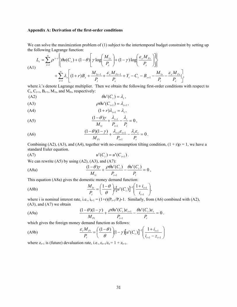
Appendix A: Derivation of the first-order conditions

We can solve the maximization problem of (1) subject to the intertemporal budget constraint by setting up the following Lagrange function:

(A1)

,)1(

log)1(log)1()(

11

111

1

−−−−+++++

−+

−+=

+−−

∞

=

∞

=

−

∑

∑

s

Fss

t

sstt

s

Fss

t

ss

tss

s

Fss

s

ss

ts

tst

PM

PM

BCYP

MP

MBr

PM

PM

CuL

εελ

εγγθθρ

where λ’s denote Lagrange multiplier. Then we obtain the following first-order conditions with respect to Ct, Ct+1, Bt+1, M1t, and MFt, respectively: (A2) ttCu λθ =)(' , (A3) 11 )(' ++ = ttCu λρθ , (A4) ttr λλ =+ +1)1( ,

(A5) 0)1(

1

1

1

=−+−

+

+

t

t

t

t

t PPMλλγθ

,

(A6) 0)1)(1(

1

11 =−+−−

+

++

t

tt

t

tt

Ft PPMελελγθ

.

Combining (A2), (A3), and (A4), together with no-consumption tilting condition, (1 + r)ρ = 1, we have a standard Euler equation. (A7) )(')(' 1+= tt CuCu . We can rewrite (A5) by using (A2), (A3), and (A7):

(A8a) 0)(')(')1(

11

=−+−

+ t

t

t

t

t PCu

PCu

Mθρθγθ

,

This equation (A8a) gives the domestic money demand function:

(A8b) [ ]

+

−

=+

+−

1

111 1)('1

t

tt

t

t

ii

CuP

Mγ

θθ

,

where i is nominal interest rate, i.e., it+1 = (1+r)(Pt+1/Pt)-1. Similarly, from (A6) combined with (A2), (A3), and (A7) we obtain

(A9a) 0)(')(')1)(1(

1

1 =−+−−

+

+

t

tt

t

tt

Ft PCu

PCu

Mεθερθγθ

.

which gives the foreign money demand function as follows:

(A9b) [ ]

−

+−

−

=++

+−

11

11 1)(')1()1(

tt

tt

t

Ftt

zii

CuPM

γθ

θε

where zt+1 is (future) devaluation rate, i.e., εt+1/εt = 1 + zt+1.

31

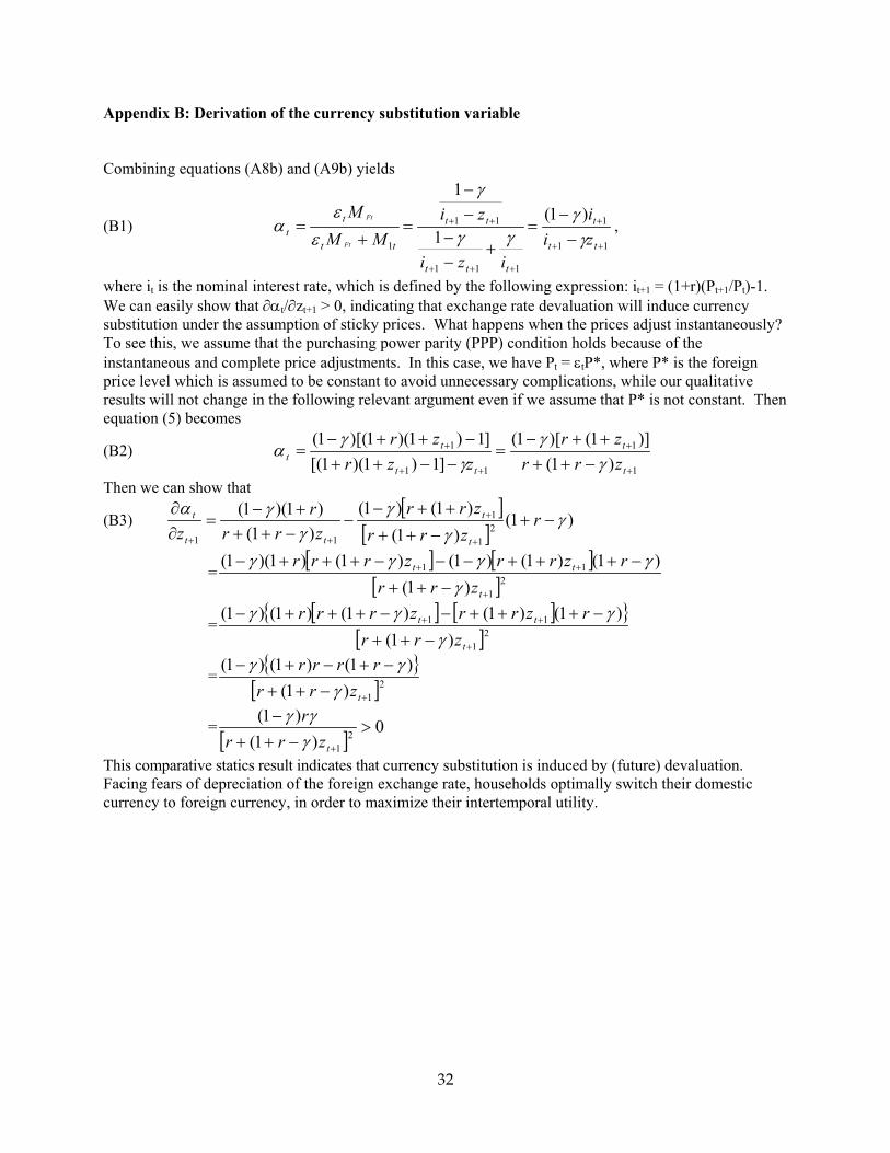
Appendix B: Derivation of the currency substitution variable Combining equations (A8b) and (A9b) yields

(B1) 11

1

111

11

1

)1(

1

1

++

+

+++

++

−−

=+

−−

−−

=+

=tt

t

ttt

tt

tt

tt zi

i

izi

ziMM

M

Ft

Ft

γγ

γγ

γ

εε

α ,

where it is the nominal interest rate, which is defined by the following expression: it+1 = (1+r)(Pt+1/Pt)-1. We can easily show that ∂αt/∂zt+1 > 0, indicating that exchange rate devaluation will induce currency substitution under the assumption of sticky prices. What happens when the prices adjust instantaneously? To see this, we assume that the purchasing power parity (PPP) condition holds because of the instantaneous and complete price adjustments. In this case, we have Pt = εtP*, where P* is the foreign price level which is assumed to be constant to avoid unnecessary complications, while our qualitative results will not change in the following relevant argument even if we assume that P* is not constant. Then equation (5) becomes

(B2) 1

1

11

1

)1()]1()[1(

]1)1)(1[(]1)1)(1)[(1(

+

+

++

+

−++++−

=−−++

−++−=

t

t

tt

tt zrr

zrzzr

zrγ

γγ

γα

Then we can show that

(B3) [ ]

[ ])1(

)1()1()1(

)1()1)(1(

21

1

11

γγ

γγ

γα−+

−++

++−−

−+++−

=∂∂

+

+

++

rzrr

zrrzrr

rz t

t

tt

t

=[ ] [ ]

[ ]21

11

)1()1()1()1()1()1)(1(

+

++

−++

−+++−−−+++−

t

tt

zrrrzrrzrrr

γγγγγ

=[ ] [ ]{ }

[ ]21

11

)1()1()1()1()1()1(

+

++

−++

−+++−−+++−

t

tt

zrrrzrrzrrr

γγγγ

={ }

[ ]21)1(

)1()1()1(

+−++−+−+−

tzrrrrrr

γγγ

=[ ]

0)1(

)1(2

1

>−++

−

+tzrrrγγγ

This comparative statics result indicates that currency substitution is induced by (future) devaluation. Facing fears of depreciation of the foreign exchange rate, households optimally switch their domestic currency to foreign currency, in order to maximize their intertemporal utility.

32

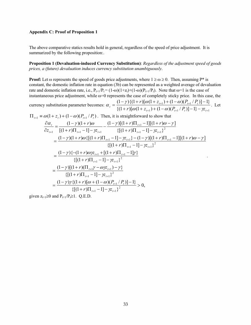
Appendix C: Proof of Proposition 1 The above comparative statics results hold in general, regardless of the speed of price adjustment. It is summarized by the following proposition:. Proposition 1 (Devaluation-induced Currency Substitution): Regardless of the adjustment speed of goods prices, a (future) devaluation induces currency substitution unambiguously. Proof: Let ω represents the speed of goods price adjustments, where 1 ≥ ω ≥ 0. Then, assuming P* is constant, the domestic inflation rate in equation (3b) can be represented as a weighted average of devaluation rate and domestic inflation rate, i.e., Pt+1/Pt = (1-ω)(1+zt)+(1-ω)(Pt+1/Pt). Note that ω=1 is the case of instantaneous price adjustment, while ω=0 represents the case of completely sticky price. In this case, the

currency substitution parameter becomes: 111

11

}1)]/)(1()1()[1{(}1)]/)(1()1()[1){(1(

+++

++

−−−+++−−+++−

=tttt

tttt zPPzr

PPzrγωω

ωωγα . Let

)/)(1()1( 11 tttt PPz ++ −++≡Π ωω . Then, it is straightforward to show that

,0}]1)1{[(

}1)]/)(1()[1{()1(

}]1)1{[(}))(1)[(1(

}]1)1{[(}]1)1[()1(){1(

}]1)1{[(])1][(1)1)[(1(}]1)1{[()1)(1(

}]1)1{[(])1][(1)1)[(1(

]1)1[()1)(1(

211

1

211

11

211

11

211

111

211

1

111

>−−Π+

−−++−=

−−Π+−−Π+−

=

−−Π+−Π+++−−

=

−−Π+−+−Π+−−−−Π++−

=

−−Π+−+−Π+−

−−−Π+

+−=

∂∂

++

+

++

++

++

++

++

+++

++

+

+++

tt

tt

tt

tt

tt

tt

tt

ttt

tt

t

ttt

t

zrPPr

zrzr

zrrzr

zrrrzrr

zrrr

zrr

z

γωωγγ

γγωγγγ

γγωγγ

γγωγγωγ

γγωγ

γωγα

.

given zt+1≥0 and Pt+1/Pt≥1. Q.E.D.

33

References

Agénor, Pierre-Richard (1994), “Credibility and Exchange Rate Management in Developing Countries,”

Journal of Development Economics, 45 (October): 1-15.

Barro, Robert J. and David B. Gordon (1983), “Rules, Discretion and Reputation in a Model of

Monetary Policy,” Journal of Monetary Economics, 12 (July): 101-121.

Blanchard, Oliver and Stanley Fischer (1989), Lectures on Macroeconomics. Cambridge, MA: MIT

Press.

Baumol, William (1952), “The Transactions Demand for Cash: An Inventory Theoretic Approach,”

Quarterly Journal of Economics, 66: 545-556.

Calvo, Guillermo A. and Carlos Végh (1996), “From Currency Substitution to Dollarization and

Beyond: Analytical and Policy Issues,” in Guillermo A. Calvo, Money, Exchange Rates and

Output. Boston, MA: MIT Press.

Calvo, Guillermo A., Leonardo Leiderman, and Carmen M. Reinhart (1993), “Capital Inflows and

Real Exchange Rate Appreciation in Latin America,” IMF Staff Papers, 40 (1): 108-151.

Cavallari, Lilia and Giancarlo Corsetti (2000), “Shadow Rates and Multiple Equilibria in the Theory of

Currency Crisis,” Journal of International Economics, 51: 275-286.

Cho, Yoon Je and Changyong Rhee (1999), “Macroeconomic Adjustment of the East Asian Economies

after the Crisis: A Comparative Study,” Seoul Journal of Economics, 12 (winter): 347-389.

Clower, Robert W. (1967), “A Reconsideration of the Microfundamentals of Monetary Theory,” Western

Economic Journal, 6: 1-19.

Cole, David C. and Betty F. Slade (1998), “The Crisis and Financial Sector Reform,” ASEAN Economic

Bulletin, 15 (3): 338-346.

Eichengreen, Barry, Andrew K. Rose, and Charles Wyplosz (1994), “Speculative Attacks on Pegged

Exchange Rates: An Empirical Exploration with Special Reference to the European Monetary

System.” NBER Working Paper No. 4898.

34

Ernst & Whinney (various years), Foreign Exchange Rates and Restrictions.

Feenstra, Robert (1986), “Functional Equivalence between Liquidity Costs and the Utility of Money,”

Journal of Monetary Economics, 17: 271-291.

Flood, Robert and Peter Garber (1984), " Collapsing Exchange Rate Regimes: Some Linear Examples,"

Journal of International Economics, 17 (August): 1-13.

Flood, Robert and Nancy P. Marion (2000), “Self-fulfilling Risk Predictions: An Application to

Speculative Attacks,” Journal of International Economics, 50: 245-268.

Frank, Robert H. (1985), Choosing the Right Pond. New York: Oxford University Press.

Frank, Robert H. and Philip J. Cook (1976), The Winner-Take-All Society: Why the Few at the Top Get

So Much More Than the Rest of Us. New York: Penguin.

Girton, Lance and Don Roper (1981), “Theory and Implications of Currency Substitution,” Journal of

Money, Credit and Banking, 13 (1): 12-30.

Giovannini, Alberto and Bart Turtelboom (1994), “Currency Substitution,” in Frederick van der Ploeg,

ed., The Handbook of International Macroeconomics. Oxford: Basil Blackwell.

Hirsh, Fred (1976), Social Limits to Growth. Cambridge, MA: Harvard University Press.

Kareken, John and Neil Wallace (1981), “On the Indeterminacy of Equilibrium Exchange Rates,”

Quarterly Journal of Economics, 96 (2): 207-222.

Keynes, John Maynard (1923), A Tract for Monetary Reform. New York: Macmillan.

Kravis, Irving B., Alan Heston and Robert Summers (1982), World Product and Income: International

Comparisons of Real Gross Product. Baltimore, MD: Johns Hopkins.

Krugman, Paul R. (1979) “A Model of Balance-of-Payments Crises,” Journal of Money, Credit and

Banking, 11: 311-25.

Lucas, Robert and Nancy L. Stokey (1987), “Money and Interest in a Cash-in-Advance Economy,”

Econometrica, 55 (May): 491-513.

McKinnon, Ronald.I. (1979), Money in International Exchange. New York: Oxford University Press.

35

Obstfeld, Maurice (1996), “Models of Currency Crisis with Self-fulfilling Features,” European

Economic Review, 40: 1037-1047.

Obstfeld, Maurice and Kenneth Rogoff (1996), Foundations of International Macroeconomics.

Cambridge, MA: MIT Press.

Pagano, Ugo (1999), “Is Power an Economic Good? Notes on Social Scarcity and the Economics of

Positional Goods,” in Samuel Bowles, Maurizio Franzini and Ugo Pagano, eds., The Politics and

Economics of Power. London: Routledge. Pp. 63-84.

Sawada, Yasuyuki (1994), “Are the Heavily Indebted Countries Solvent? Tests of Intertemporal Budget

Constraints,” Journal of Development Economics, 45: 325-337.

Sawada, Yasuyuki (2001), “Secondary Market Efficiency for LDC Bank Loans and International Private

Lending, 1985-1993,” Journal of International Money and Finance, 20: 549-562.

Sidrauski, Miguel (1967), “Rational Choice and Patterns of Growth in a Monetary Economy,” American

Economic Review, 57 (2): 534-544.

Stiglitz, Joseph E. and Andrew Weiss (1981), "Credit Rationing in Markets with Imperfect

Information," American Economic Review, 71 (June): 393-410.

Summers, Robert and Alan Heston (1991), “The Penn World Table (Mark 5): An Expanded Set of

International Comparisons, 1950-1988,” Quarterly Journal of Economics, 106 (May): 327-368.

Homepage: http://pwt.econ.upenn.edu

Tobin, James (1956), “The Interest Rate Elasticity of Transactions Demand for Cash,” Review of

Economics and Statistics, 38: 241-247.

Uribe, Martin (1997), “Hysteresis in a Simple Model of Currency Substitution,” Journal of Monetary

Economics 40, 185-202.

Wood, Adrian (1999), "Data on Black Market Premium." University of Sussex, Institute of Development

Studies (Compact Disk).

Yotopoulos, Pan A. (1996), Exchange Rate Parity for Trade and Development: Theory, Tests, and Case

36

Studies. London and New York: Cambridge University Press.

Yotopoulos, Pan A. (1997), “Financial Crises and the Benefits of Mildly Repressed Exchange Rates.”

Stockholm School of Economics Working Paper Series in Economics and Finance, No. 202

(October).

Yotopoulos, Pan A. and Yasuyuki Sawada (1999), “Free Currency Markets, Financial Crises and the

Growth Debacle: Is There a Causal Relationship?” Seoul Journal of Economics, 12 (winter): 419-

456..

37

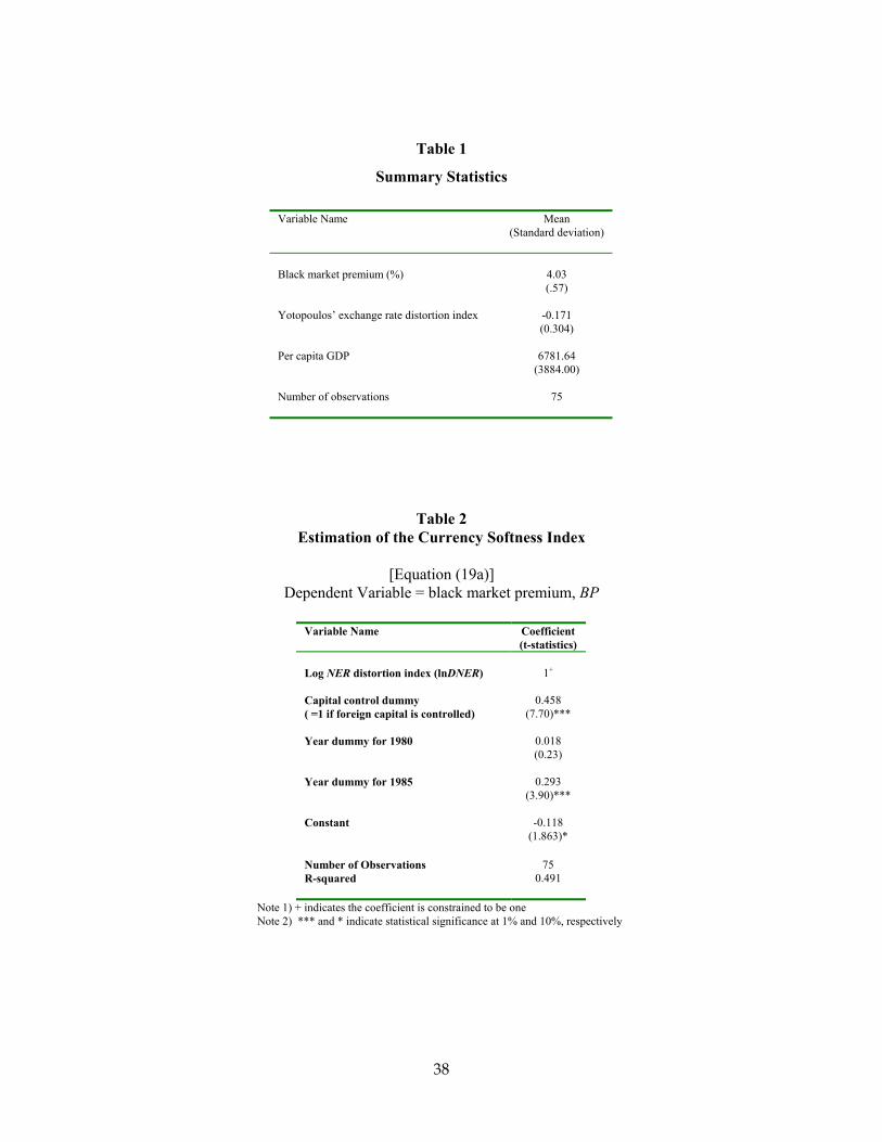
Table 1

Summary Statistics

Variable Name Mean (Standard deviation)

Black market premium (%)

4.03 (.57)

Yotopoulos’ exchange rate distortion index

-0.171 (0.304)

Per capita GDP

6781.64

(3884.00) Number of observations

75

Table 2 Estimation of the Currency Softness Index

[Equation (19a)]

Dependent Variable = black market premium, BP

Variable Name Coefficient (t-statistics)

Log NER distortion index (lnDNER) 1+ Capital control dummy ( =1 if foreign capital is controlled)

0.458

(7.70)***

Year dummy for 1980 0.018 (0.23)

Year dummy for 1985

0.293

(3.90)*** Constant

-0.118

(1.863)*

Number of Observations 75 R-squared 0.491

Note 1) + indicates the coefficient is constrained to be one Note 2) *** and * indicate statistical significance at 1% and 10%, respectively

38

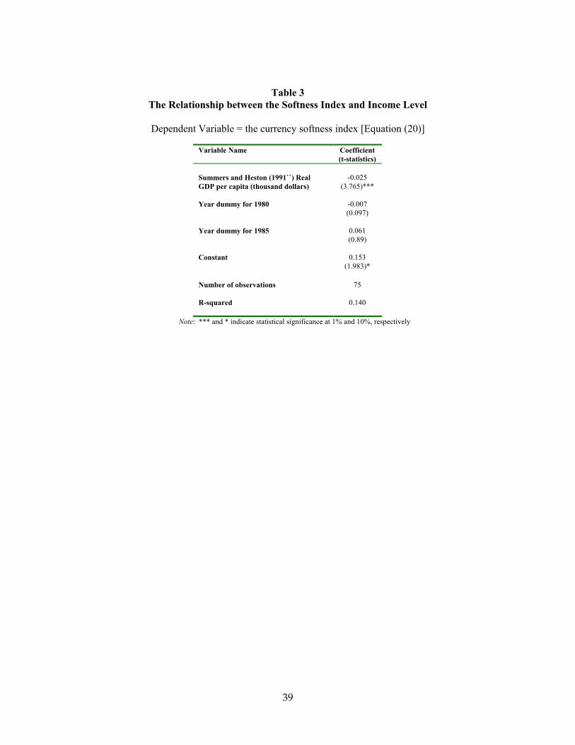
Table 3 The Relationship between the Softness Index and Income Level

Dependent Variable = the currency softness index [Equation (20)]

Variable Name Coefficient (t-statistics)

Summers and Heston (1991``) Real GDP per capita (thousand dollars)

-0.025

(3.765)*** Year dummy for 1980

-0.007 (0.097)

Year dummy for 1985

0.061 (0.89)

Constant

0.153

(1.983)*

Number of observations 75 R-squared

0.140

Note: *** and * indicate statistical significance at 1% and 10%, respectively

39

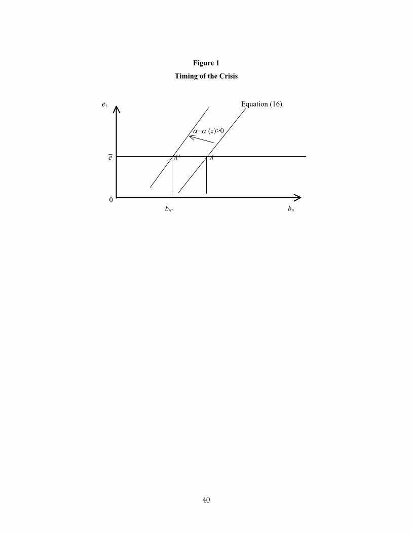
Figure 1

Timing of the Crisis

eT Equation (16)

α=α (z)>0

e A’ A

0 bHT bH

40

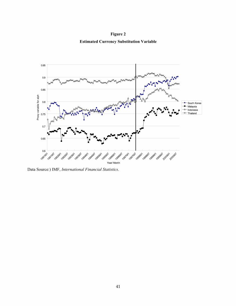
Figure 2

Estimated Currency Substitution Variable

0.6

0.65

0.7

0.75

0.8

0.85

0.9

0.95

1991

M1

1991

M7

1992

M1

1992

M7

1993

M1

1993

M7

1994

M1

1994

M7

1995

M1

1995

M7

1996

M1

1996

M7

1997

M1

1997

M7

1998

M1

1998

M7

1999

M1

1999

M7

2000

M1

2000

M7

Year/ Month

Prox

y va

riabl

e fo

r alp

h

South KoreaMalaysiaIndonesiaThailand

Data Source:) IMF, International Financial Statistics.

41

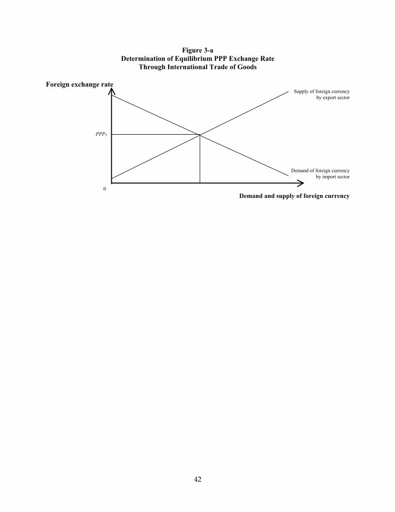
Figure 3-a Determination of Equilibrium PPP Exchange Rate

Through International Trade of Goods

Foreign exchange rate Supply of foreign currency

by export sector

PPPT

Demand of foreign currency by import sector

0

Demand and supply of foreign currency

42

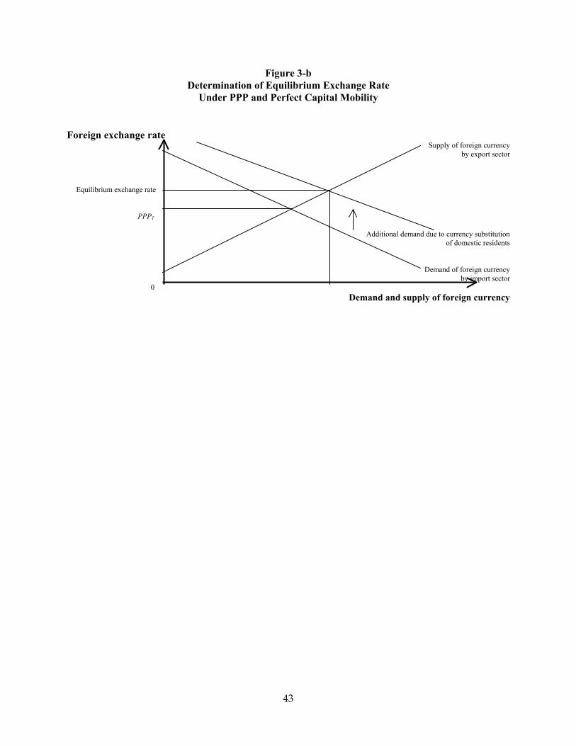
Figure 3-b Determination of Equilibrium Exchange Rate

Under PPP and Perfect Capital Mobility

Foreign exchange rate Supply of foreign currency

by export sector

Equilibrium exchange rate

PPPT

Additional demand due to currency substitution

of domestic residents

Demand of foreign currency by import sector

0 Demand and supply of foreign currency

43

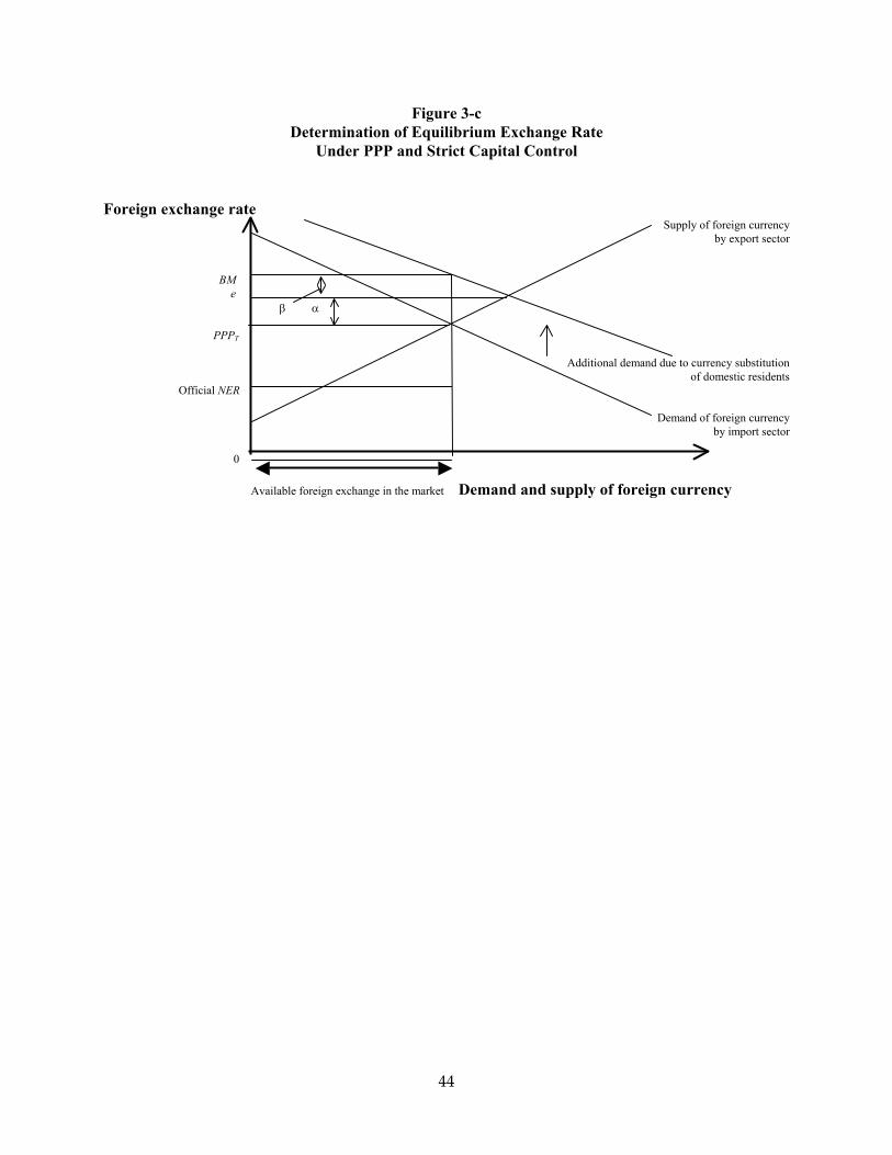
Figure 3-c Determination of Equilibrium Exchange Rate

Under PPP and Strict Capital Control

Foreign exchange rate Supply of foreign currency

by export sector

BM e β α

PPPT

Additional demand due to currency substitution

of domestic residents Official NER

Demand of foreign currency

by import sector 0 Available foreign exchange in the market Demand and supply of foreign currency

44

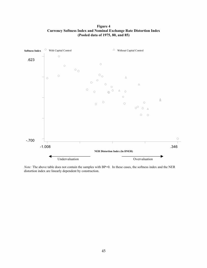
Figure 4 Currency Softness Index and Nominal Exchange Rate Distortion Index

(Pooled data of 1975, 80, and 85)

Softness Index

NER Distortion Index (ln DNER)

With Capital Control Without Capital Control

-1.008 .346-.700

.623

Undervaluation Overvaluation Note: The above table does not contain the samples with BP=0. In these cases, the softness index and the NER distortion index are linearly dependent by construction.

45

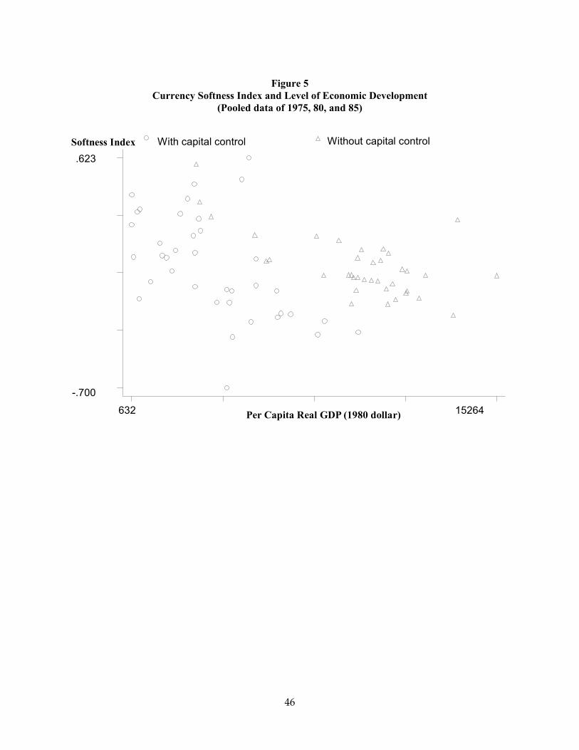
Figure 5 Currency Softness Index and Level of Economic Development

(Pooled data of 1975, 80, and 85)

Softness Index

Per Capita Real GDP (1980 dollar)

With capital control Without capital control

632 15264

-.700

.623

46

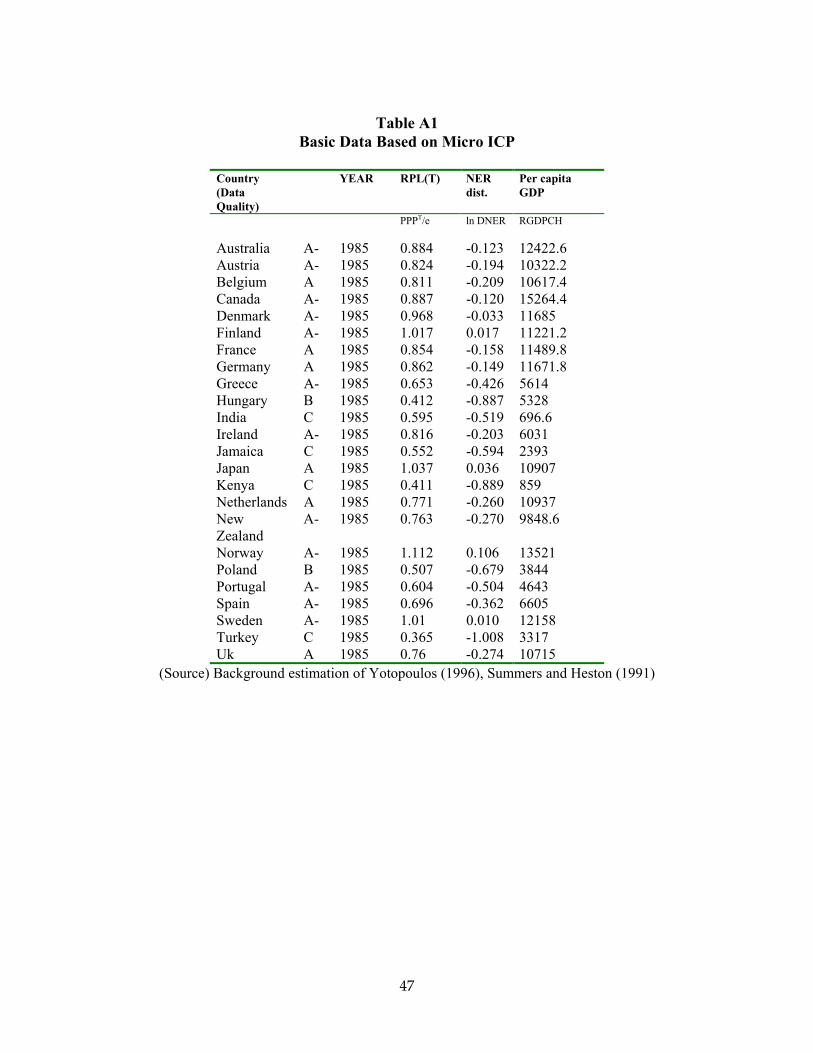
Table A1 Basic Data Based on Micro ICP

Country (Data Quality)

YEAR RPL(T) NER dist.

Per capita GDP

PPPT/e ln DNER RGDPCH

Australia A- 1985 0.884 -0.123 12422.6 Austria A- 1985 0.824 -0.194 10322.2 Belgium A 1985 0.811 -0.209 10617.4 Canada A- 1985 0.887 -0.120 15264.4 Denmark A- 1985 0.968 -0.033 11685 Finland A- 1985 1.017 0.017 11221.2 France A 1985 0.854 -0.158 11489.8 Germany A 1985 0.862 -0.149 11671.8 Greece A- 1985 0.653 -0.426 5614 Hungary B 1985 0.412 -0.887 5328 India C 1985 0.595 -0.519 696.6 Ireland A- 1985 0.816 -0.203 6031 Jamaica C 1985 0.552 -0.594 2393 Japan A 1985 1.037 0.036 10907 Kenya C 1985 0.411 -0.889 859 Netherlands A 1985 0.771 -0.260 10937 New Zealand

A- 1985 0.763 -0.270 9848.6

Norway A- 1985 1.112 0.106 13521 Poland B 1985 0.507 -0.679 3844 Portugal A- 1985 0.604 -0.504 4643 Spain A- 1985 0.696 -0.362 6605 Sweden A- 1985 1.01 0.010 12158 Turkey C 1985 0.365 -1.008 3317 Uk A 1985 0.76 -0.274 10715

(Source) Background estimation of Yotopoulos (1996), Summers and Heston (1991)

47

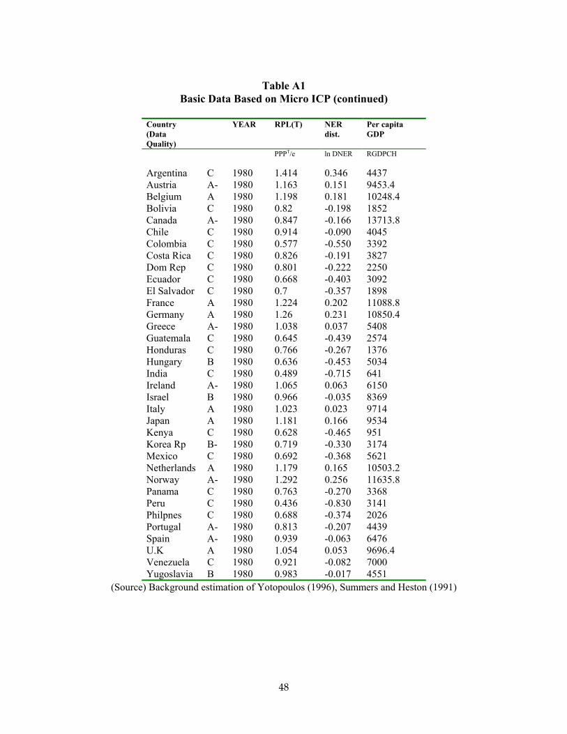
Table A1 Basic Data Based on Micro ICP (continued)

Country (Data Quality)

YEAR RPL(T) NER dist.

Per capita GDP

PPPT/e ln DNER RGDPCH

Argentina C 1980 1.414 0.346 4437 Austria A- 1980 1.163 0.151 9453.4 Belgium A 1980 1.198 0.181 10248.4 Bolivia C 1980 0.82 -0.198 1852 Canada A- 1980 0.847 -0.166 13713.8 Chile C 1980 0.914 -0.090 4045 Colombia C 1980 0.577 -0.550 3392 Costa Rica C 1980 0.826 -0.191 3827 Dom Rep C 1980 0.801 -0.222 2250 Ecuador C 1980 0.668 -0.403 3092 El Salvador C 1980 0.7 -0.357 1898 France A 1980 1.224 0.202 11088.8 Germany A 1980 1.26 0.231 10850.4 Greece A- 1980 1.038 0.037 5408 Guatemala C 1980 0.645 -0.439 2574 Honduras C 1980 0.766 -0.267 1376 Hungary B 1980 0.636 -0.453 5034 India C 1980 0.489 -0.715 641 Ireland A- 1980 1.065 0.063 6150 Israel B 1980 0.966 -0.035 8369 Italy A 1980 1.023 0.023 9714 Japan A 1980 1.181 0.166 9534 Kenya C 1980 0.628 -0.465 951 Korea Rp B- 1980 0.719 -0.330 3174 Mexico C 1980 0.692 -0.368 5621 Netherlands A 1980 1.179 0.165 10503.2 Norway A- 1980 1.292 0.256 11635.8 Panama C 1980 0.763 -0.270 3368 Peru C 1980 0.436 -0.830 3141 Philpnes C 1980 0.688 -0.374 2026 Portugal A- 1980 0.813 -0.207 4439 Spain A- 1980 0.939 -0.063 6476 U.K A 1980 1.054 0.053 9696.4 Venezuela C 1980 0.921 -0.082 7000 Yugoslavia B 1980 0.983 -0.017 4551

(Source) Background estimation of Yotopoulos (1996), Summers and Heston (1991)

48

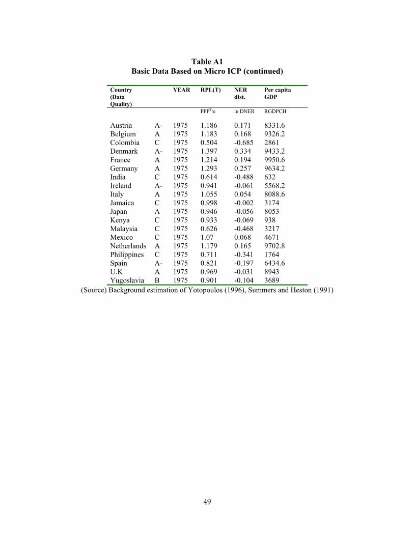
Table A1

Basic Data Based on Micro ICP (continued)

Country (Data Quality)

YEAR RPL(T) NER dist.

Per capita GDP

PPPT/e ln DNER RGDPCH

Austria A- 1975 1.186 0.171 8331.6 Belgium A 1975 1.183 0.168 9326.2 Colombia C 1975 0.504 -0.685 2861 Denmark A- 1975 1.397 0.334 9433.2 France A 1975 1.214 0.194 9950.6 Germany A 1975 1.293 0.257 9634.2 India C 1975 0.614 -0.488 632 Ireland A- 1975 0.941 -0.061 5568.2 Italy A 1975 1.055 0.054 8088.6 Jamaica C 1975 0.998 -0.002 3174 Japan A 1975 0.946 -0.056 8053 Kenya C 1975 0.933 -0.069 938 Malaysia C 1975 0.626 -0.468 3217 Mexico C 1975 1.07 0.068 4671 Netherlands A 1975 1.179 0.165 9702.8 Philippines C 1975 0.711 -0.341 1764 Spain A- 1975 0.821 -0.197 6434.6 U.K A 1975 0.969 -0.031 8943 Yugoslavia B 1975 0.901 -0.104 3689

(Source) Background estimation of Yotopoulos (1996), Summers and Heston (1991)

49

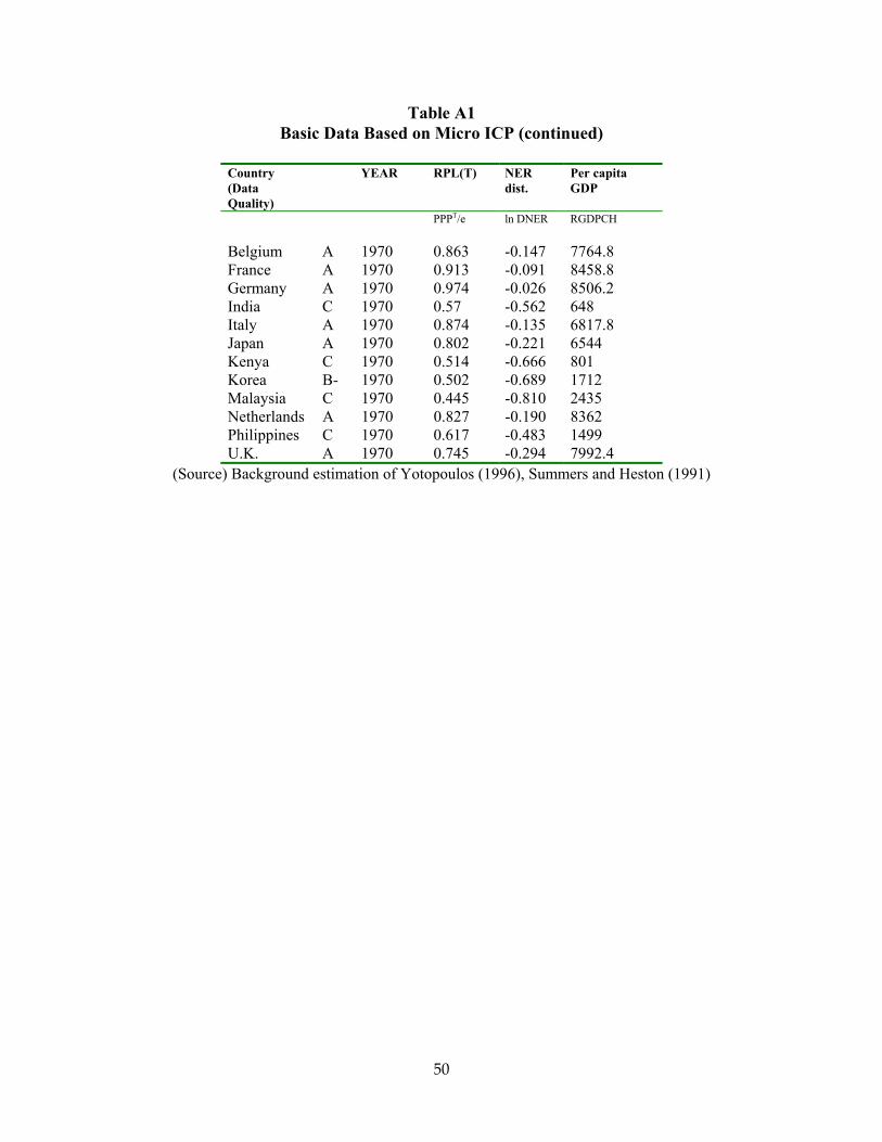
Table A1 Basic Data Based on Micro ICP (continued)

Country (Data Quality)

YEAR RPL(T) NER dist.

Per capita GDP

PPPT/e ln DNER RGDPCH

Belgium A 1970 0.863 -0.147 7764.8 France A 1970 0.913 -0.091 8458.8 Germany A 1970 0.974 -0.026 8506.2 India C 1970 0.57 -0.562 648 Italy A 1970 0.874 -0.135 6817.8 Japan A 1970 0.802 -0.221 6544 Kenya C 1970 0.514 -0.666 801 Korea B- 1970 0.502 -0.689 1712 Malaysia C 1970 0.445 -0.810 2435 Netherlands A 1970 0.827 -0.190 8362 Philippines C 1970 0.617 -0.483 1499 U.K. A 1970 0.745 -0.294 7992.4

(Source) Background estimation of Yotopoulos (1996), Summers and Heston (1991)

50

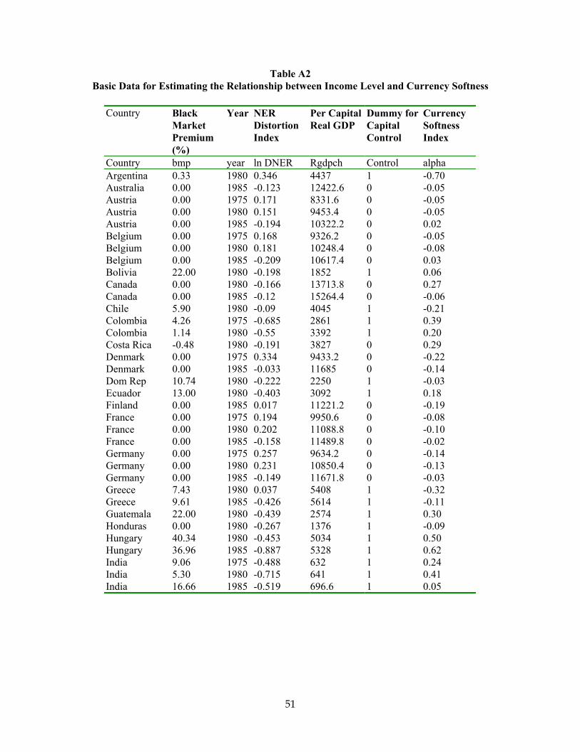
Table A2 Basic Data for Estimating the Relationship between Income Level and Currency Softness

Country Black Market Premium (%)

Year NER Distortion Index

Per Capital Real GDP

Dummy for Capital Control

Currency Softness Index

Country bmp year ln DNER Rgdpch Control alpha Argentina 0.33 1980 0.346 4437 1 -0.70 Australia 0.00 1985 -0.123 12422.6 0 -0.05 Austria 0.00 1975 0.171 8331.6 0 -0.05 Austria 0.00 1980 0.151 9453.4 0 -0.05 Austria 0.00 1985 -0.194 10322.2 0 0.02 Belgium 0.00 1975 0.168 9326.2 0 -0.05 Belgium 0.00 1980 0.181 10248.4 0 -0.08 Belgium 0.00 1985 -0.209 10617.4 0 0.03 Bolivia 22.00 1980 -0.198 1852 1 0.06 Canada 0.00 1980 -0.166 13713.8 0 0.27 Canada 0.00 1985 -0.12 15264.4 0 -0.06 Chile 5.90 1980 -0.09 4045 1 -0.21 Colombia 4.26 1975 -0.685 2861 1 0.39 Colombia 1.14 1980 -0.55 3392 1 0.20 Costa Rica -0.48 1980 -0.191 3827 0 0.29 Denmark 0.00 1975 0.334 9433.2 0 -0.22 Denmark 0.00 1985 -0.033 11685 0 -0.14 Dom Rep 10.74 1980 -0.222 2250 1 -0.03 Ecuador 13.00 1980 -0.403 3092 1 0.18 Finland 0.00 1985 0.017 11221.2 0 -0.19 France 0.00 1975 0.194 9950.6 0 -0.08 France 0.00 1980 0.202 11088.8 0 -0.10 France 0.00 1985 -0.158 11489.8 0 -0.02 Germany 0.00 1975 0.257 9634.2 0 -0.14 Germany 0.00 1980 0.231 10850.4 0 -0.13 Germany 0.00 1985 -0.149 11671.8 0 -0.03 Greece 7.43 1980 0.037 5408 1 -0.32 Greece 9.61 1985 -0.426 5614 1 -0.11 Guatemala 22.00 1980 -0.439 2574 1 0.30 Honduras 0.00 1980 -0.267 1376 1 -0.09 Hungary 40.34 1980 -0.453 5034 1 0.50 Hungary 36.96 1985 -0.887 5328 1 0.62 India 9.06 1975 -0.488 632 1 0.24 India 5.30 1980 -0.715 641 1 0.41 India 16.66 1985 -0.519 696.6 1 0.05

51

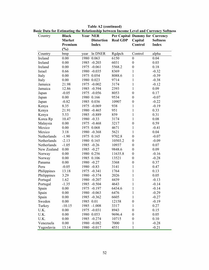
52

Table A2 (continued) Basic Data for Estimating the Relationship between Income Level and Currency Softness

Country Black Market Premium (%)

Year NER Distortion Index

Per Capital Real GDP

Dummy for Capital Control

Currency Softness Index

Country bmp year ln DNER Rgdpch Control alpha Ireland 0.00 1980 0.063 6150 0 0.04 Ireland 0.00 1985 -0.203 6031 0 0.03 Ireland 0.00 1975 -0.061 5568.2 0 0.18 Israel 0.66 1980 -0.035 8369 1 -0.32 Italy 0.00 1975 0.054 8088.6 1 -0.39 Italy 0.00 1980 0.023 9714 1 -0.38 Jamaica 21.98 1975 -0.002 3174 1 -0.12 Jamaica 12.86 1985 -0.594 2393 1 0.09 Japan -0.05 1975 -0.056 8053 0 0.17 Japan 0.00 1980 0.166 9534 0 -0.07 Japan -0.82 1985 0.036 10907 0 -0.22 Kenya 8.35 1975 -0.069 938 1 -0.19 Kenya 21.91 1980 -0.465 951 1 0.33 Kenya 5.53 1985 -0.889 859 1 0.31 Korea Rp 10.47 1980 -0.33 3174 1 0.08 Malaysia 0.00 1975 -0.468 3217 0 0.59 Mexico 0.00 1975 0.068 4671 1 -0.41 Mexico 3.18 1980 -0.368 5621 1 0.04 Netherlands -1.90 1975 0.165 9702.8 0 -0.07 Netherlands -2.13 1980 0.165 10503.2 0 -0.09 Netherlands -1.05 1985 -0.26 10937 0 0.07 New Zealand 0.00 1985 -0.27 9848.6 0 0.09 Norway 0.00 1980 0.256 11635.8 0 -0.16 Norway 0.00 1985 0.106 13521 0 -0.28 Panama 0.00 1980 -0.27 3368 0 0.37 Peru -0.05 1980 -0.83 3141 1 0.47 Philippines 13.18 1975 -0.341 1764 1 0.13 Philippines 3.29 1980 -0.374 2026 1 0.05 Portugal 1.62 1980 -0.207 4439 1 -0.13 Portugal -1.35 1985 -0.504 4643 1 -0.14 Spain 0.00 1975 -0.197 6434.6 1 -0.14 Spain 0.00 1980 -0.063 6476 1 -0.29 Spain 0.00 1985 -0.362 6605 1 -0.27 Sweden 0.00 1985 0.01 12158 0 -0.19 Turkey -10.15 1985 -1.008 3317 1 0.27 U.K. 0.00 1975 -0.031 8943 0 0.15 U.K. 0.00 1980 0.053 9696.4 0 0.05 U.K. 0.00 1985 -0.274 10715 0 0.10 Venezuela 0.00 1980 -0.082 7000 1 -0.28 Yugoslavia 13.14 1980 -0.017 4551 1 -0.21