21/1/2006

Currency Substitution, Portfolio

Diversification and Money Demand

Miguel Lebre de Freitas

Universidade de Aveiro and NIPE

Departamento de Economia, Gestão e Engenharia Industrial

Campus Universitário, 3810-193 Aveiro, Portugal.

Tel: 351-234-370200. Fax: 351-234-370215. E-mail: afreitas@egi.ua.pt

Francisco José Veiga

Universidade do Minho and NIPE

Escola de Economia e Gestão

4710-057 Braga, Portugal

Tel: +351-253604534. Fax: +351-253676375. Email: fjveiga@eeg.uminho.pt

1

Currency Substitution, Portfolio

Diversification and Money Demand

Miguel Lebre de Freitas - Universidade de Aveiro and NIPE

Francisco José Veiga - Universidade do Minho and NIPE

We extend the Thomas (1985) dynamic optimising model of money demand and

currency substitution to the case in which the individual has restricted or no access

to foreign currency denominated bonds. In this case Currency Substitution decisions

and Asset Substitution decisions are not separable. The results obtained suggest that

the significance of an expected exchange rate depreciation term in the demand for

domestic money provides a valid test for the presence of currency substitution.

Applying this approach to six Latin American countries, we find evidence of currency

substitution in Colombia, Dominican Republic and Venezuela, but not in Brazil and

Chile.

JEL Classification: E41, F41, G11.

Keywords: Money Demand, Currency Substitution, Dollarisation, Portfolio Choice.

2

1. Introduction

During periods of macroeconomic and political uncertainty, many developing

countries experience a partial replacement of the domestic currency by a foreign

currency either as store of value, unit of account or means of payment. The latter case

is usually referred to as “Currency Substitution”. Currency Substitution is a demand

driven process that results from means of payment substitutability (though it is not

necessarily implied by it) and shall be distinguished from the broader concept of

“Asset Substitution” (or “Dollarisation”), which refers to the switching from

(monetary and non-monetary) assets denominated in domestic currency to (monetary

and non-monetary) assets denominated in foreign currency1.

This paper examines the implications of imperfect means of payment

substitutability on the properties of the money demand, using a stochastic dynamic

optimising model in which the specific role of money is explicitly accounted for. In

particular, it is assumed that money reduces the frictional losses from transacting in

the goods market. This feature of the model is essential to distinguish the

phenomenon of Currency Substitution (CS) from Asset Substitution (AS). This paper

compares two alternative assumptions concerning capital mobility: first, the case in

which the consumer has unrestricted access to nominally riskless bonds denominated

in foreign currency and then the case in which the consumer faces a binding

restriction on foreign bond holdings. In both cases, the individual is allowed to hold

an interest-bearing asset denominated in domestic currency paying a certain nominal

return.

3

The first case draws on Thomas (1985). This author demonstrated that

borrowing and lending opportunities separate CS decisions from AS decisions. Since

money bears the same characteristics as (same currency) bonds and earns a lower

return, it should not be held in the portfolio for the speculative and risk-

diversification reasons that underlie the demand for financial assets in general

(Thomas, 1985, pp 354: “in a model with a complete set of nominally riskless bonds

there is no demand for money as a portfolio asset”). In this context, domestic and

foreign money holdings are selected solely to satisfy transaction needs. The optimal

denomination structure of the overall portfolio (AS), in turn, shall reflect a balance

between expected returns and currency risk. Through borrowing and lending, the

individual is able to achieve the optimal level of AS, independently of his choice

among monetary assets (CS).

Thomas’ separation result depends critically on the assumption that bond

markets are complete. As pointed out by Cuddington (1989), such an assumption may

not be suitable to describe the demand for money in countries with imperfect capital

mobility. The contribution of this paper is to extend the Thomas (1985) model to the

case in which the consumer has restricted or no access to bonds denominated in

foreign currency. This is the appropriate set-up to describe the demand for money in

economies subject to capital controls or in economies where openness of capital

markets has not reached a significant part of the population.

The implication of introducing a binding constraint on foreign bond holdings is

that foreign money assumes a store of value role, in addition to its eventual means of

payment role. The double role that foreign money balances may have under asset

4

holding constraints and CS is formally described in this paper. We show that if the

domestic and foreign monies are substitutes as means of payment, then the demand

for domestic money will be influenced by speculative and risk-hedging decisions.

This is not to say that domestic money will be demanded as a “portfolio asset”: since

domestic money is dominated by an interest-bearing asset, its demand will be driven

by transactions purposes only. Means of payment substitutability, however, opens a

channel through which the optimal choice between assets denominated in different

currencies impacts on the liquidity value of the domestic money. In this context,

separation of CS decisions and AS decisions no longer holds.

The money demand properties in this model are, thus, different from those

postulated by the Portfolio Balance Approach to Currency Substitution (Cuddington,

1983). In light of that theory, money is viewed as a simple asset, that is gross

substitute of all other available assets. In a context where foreign money and foreign

bonds are both available, this leads to a demand for domestic money that depends

negatively on the expected exchange rate depreciation by two different channels:

substitution vis-à-vis the foreign money (currency substitution) and substitution vis-à-

vis the foreign bond (capital flight). For this reason, followers of the Portfolio

Balance Approach have argued that the significance of an expected exchange rate

depreciation term in the demand for domestic money does not provide a valid test for

the presence of CS. In contrast to that theory, the model explored in this paper allows

domestic and foreign monies to be substitutes for transactions, while their relevance

as store of value depends on the availability of like-denominated bonds. We show

that only in the case where the two monies are substitutes as means of payment will

the demand for domestic money depart from the closed economy specification.

5

Moreover, our results give support to the procedure of testing for the presence of CS

by assessing the significance of an expected exchange rate depreciation term in the

demand for domestic money.

A well-known limitation in the empirical analysis of CS is that data on foreign

banknotes held by the public are not easily available. For this reason, many authors

have proxied the demand for foreign money by the amount of foreign currency

deposits held by residents in the banking system. Other authors have developed

methodologies to estimate the amount of foreign money held by the public. This

includes estimates based on the currency denomination of loans, on postulated money

velocities or on reports of shipments of dollar bank notes from the U.S. to these

countries (see Krueger and Ha, 1996, for a survey). Irrespective of the quality of

these measures, they all face a fundamental limitation: wherever capital markets are

not well developed and there is nominal instability, the demand for foreign money

may mostly reflect a store of value motive. Thus, even if an accurate estimate of the

demand for foreign money was available, this would tell us nothing of the extent to

which foreign money was replacing domestic money as vehicle for transactions. If,

according to our results, the presence of CS can be assessed estimating a demand

function for domestic money, then this limitation is circumvented.

This paper focuses on the particular case of “asymmetric” CS, in which a local

currency is replaced by a foreign currency as vehicle for transactions in the domestic

economy. This case shall be distinguished from "international CS", which refers to

the competition among international currencies in the global economy (for the

functions of international currencies, see Krugman, 1984). This model shares with

6

Thomas (1985) the fact that only imperfect means of payment substitutability is

allowed for2. The implications of perfect means of payment substitutability are

discussed in Kareken and Wallace (1981), for the case in which agents face no

binding restrictions on money holdings, and in Lebre de Freitas (2004), for the

“asymmetric” case in which foreign residents cannot hold domestic money. Models

postulating imperfect substitutability in the provision of transaction services include

Agénor and Khan (1996), Rogers (1990) and Végh (1989). Since these models

assume away uncertainty, however, they cannot describe the speculative and risk

hedging considerations that drive the demand for foreign money in high inflation

countries. Imrohoroglu (1994) and Smith (1995) extend the analysis to a stochastic

framework, but they do not explore the properties of the money demand under asset

market restrictions. Sahay and Végh (1996) refer to the Thomas (1985) model to

describe a case in which individuals have no access to bonds denominated in foreign

currency. However, in their framework, individuals are allowed to hold interest

bearing foreign currency deposits, which play the role of the missing bond in the

model. Hence, their analysis does not depart from the original Thomas (1985) model.

A recent debate on the empirical implications of different institutional set-ups

concerning the availability of assets denominated in foreign currency may be seen in

Whited (2004) and Alami (2004). However, these authors follow the aggregative

tradition of postulating money demand functions that depend on income and

opportunity costs, rather than deriving the money demand properties from individual

optimisation.

The paper proceeds as follows: The basic model is presented in Section 2. The

money demand properties under imperfect means of payment substitutability and

7

complete bond markets are discussed in Section 3. The case in which the consumer

faces a binding constraint on foreign bond holdings is examined in Section 4. The

empirical implications of the results obtained are addressed in Section 5. In Section 6,

money-demand functions for six Latin American countries are estimated for a period

during which they imposed restrictions on capital flows, and one checks whether or

not there is empirical support for currency substitution in each country. The

conclusions are presented in Section 7.

2. The model

Consider an infinitely lived consumer, living in a small open economy. There is

only one (non-storable) consumption good, with domestic price equal to P. The

consumer is endowed with a constant flow of the good, denoted by y. She maximises

the expected value of a discounted sum of instantaneous utility functions of the form:

dtc

eo

tt∫∞ −

−

−Ε

φ

φβ

1

1

, (1)

where ct denotes real consumption at time t, β is a positive and constant subjective

discount rate, and 0>φ is the Arrow-Pratt measure of relative risk aversion.

The individual has unrestricted access to domestic money (called peso, M),

foreign money (dollar, F) and bonds denominated in domestic currency (A). Bonds

denominated in foreign currency (B) may or may not be freely available, depending

on the institutional framework under consideration. In Section 3, we discuss the

8

unrestricted case. The case with restrictions on bond availability is discussed in

Section 4. The individual's real wealth is defined as3:

bafmw +++= , (2)

where PMm = , PEFf = , PAa = , PEBb = , P is the domestic price level, and

E is the price of the dollar in peso-units.

Domestic and foreign bonds have certain nominal returns, represented by i and

j, respectively. Money holdings earn zero nominal returns. There is uncertainty

concerning the inflation rate and, hence, on real returns. The consumer takes the

inflation rate as given, because individually she cannot influence the price level. She

may, however, perceive the price level and the exchange rate to be correlated. To

capture this, it is assumed that the domestic price level and the exchange rate evolve

stochastically, according to4:

dZdtP

dP σπ += , (3)

and

dXdtE

dE γε += , (4)

where dZ and dX are standard Wiener processes with instantaneous correlation equal

to r. Denoting the covariance between the stochastic processes (3) and (4) as

rσγρ = , and using Ito's lemma, the real returns to domestic bonds, domestic money,

foreign bonds and foreign money are obtained:

( ) dZdtiada σπσ −−+= 2 , (5)

9

( ) dZdtmdm σπσ −−= 2 , (6)

( ) dXdZdtjbdb γσρπσε +−−−++= 2 , (7)

( ) dXdZdtf

df γσρπσε +−−−+= 2 . (8)

Money is distinguished from bonds in that it provides liquidity services. We

assume that money reduces frictional losses from transacting in the goods markets5.

Purchases of the consumption good are subject to a transaction cost (τ), that depends

positively on the real consumption level (c) and negatively on the amount of real

money balances. To allow for CS, it is assumed that both the domestic money and the

foreign money serve as means of payment. For simplicity, we will refer to a particular

transactions technology, introduced by Végh (1989):

Assumption 1. (The transactions technology): τ(.) is a non-negative, twice

continuously differentiable and convex function of the form:

⎥⎦⎤

⎢⎣⎡=

cf

cmcv ,τ , (9)

with 0(.) >v , 01 <v , 02 <v , 011 >v , 022 >v , 012 ≥v and 02122211 >−=Δ vvv .

In (9), τ refers to the amount of real resources spent in transacting, and a

subscript k (k=1,2) to the function v(.) denotes partial differentiation with respect to

the k argument. Linear homogeneity and the assumption that additional real money

balances (either domestic or foreign) bring about diminishing reductions in

transaction costs are not necessary for the main propositions to hold, but help,

10

respectively, to simplify the algebra and to assure well behaved money demand

functions6.

The fact that foreign money provides liquidity services does not necessarily

imply means of payment substitutability. Suppose, for example, that some fraction of

the consumption bundle is purchased using pesos only, and that the remaining

fraction is purchased using dollars only. In this case, there is no substitutability.

Means of payment substitutability occurs when some fraction of the consumption

bundle can be purchased with money denominated in either currency. In that case,

one might expect the effect on transaction costs of increasing the holdings of one

money to depend negatively on the holdings of the other money. Formally, this can

be stated in the following way:

Definition 1. (Means of payment substitutability): the domestic and foreign

monies are said to be substitutes as means of payment if the cross derivative 12v in

equation (9) is strictly positive.

The consumer’s flow budget constraint depends on the amount of saved wealth

allocated to the available assets and on real returns:

( )[ ]dtcydbdadfdmdw .τ−−++++= . (10)

Using (2), (9) and (5)-(8), the flow budget constraint becomes:

( ) dZwdXfbdtdw σγ −++Φ= , (11)

with =Φ

( ) ( ) ( )( )( )[ ].1)( 2

222

vcybjbfmwifm

+−+−−+++

−−−−++−−++−=

ρπσε

πσρπσεπσ

11

The consumer problem is to maximise (1), subject to the stochastic

differential (11). To account for restrictions on foreign bond holdings, we formulate

the problem assuming that b is confined to the following control set:

0≥− bb (12)

This constraint will be assumed to be binding or not, depending on the

institutional framework under consideration. The Hamilton-Jacobi-Bellman equation

of the corresponding quasi-stationary problem is:

( ) ( )[ ]⎭⎬⎫

⎩⎨⎧

+−+++Φ+−

=−

≤ρσσγ

φβ

φ

fbwwfbwVwVcwVbbfmc

2)(''21)('

1max)( 2222

1

,,,

where Φ is defined as in (11) and V(w) is the optimal value function. The first order

conditions in respect to b, f and m may be stated in the following way:

[ ] ( )[ ] 0)´´()(' 2 =−−+++−− λργρε wfbwVjiwV (13)

[ ] ( )[ ] 0)´´()(' 22 =−++−−− ργρε wfbwVviwV (14)

0,1 =⎟⎠⎞

⎜⎝⎛+

cf

cmvi , (15)

where 0≥λ is the Lagrangian multiplier associated to the constraint (12). Condition

(13) accounts for both interior solutions and a boundary solution for b: according to

the Khun-Tucker complementary slackness conditions, if the constraint (12) is not

binding, then λ=0. If, instead, constraint (12) is binding, then λ>0 , meaning that

lessening the constraint would have a positive impact on the optimal value function.

These two cases are discussed in the following sections.

12

3. The case with complete bond markets (Thomas, 1985)

In this section, we examine the case in which foreign bonds are freely available.

In terms of the formulation above, this case is accounted for by postulating a large

enough value for b , so as to ensure that restriction (12) is not binding. Substituting

λ=0 in (13) and subtracting from (14), one obtains:

0,2 =⎟⎠⎞

⎜⎝⎛+

cf

cmvj . (16)

Using )(')('' wVwwV−=φ in (13) with λ=0 and rearranging, one obtains:

⎟⎟⎠

⎞⎜⎜⎝

⎛⎟⎟⎠

⎞⎜⎜⎝

⎛−+⎟⎟

⎠

⎞⎜⎜⎝

⎛ −+⎟⎟⎠

⎞⎜⎜⎝

⎛=

+22

111γρ

φγε

φij

wfb , (17)

Equation (17) is the well known optimal portfolio rule in a world with two

assets (see Branson and Henderson, 1985, for a survey). It states that the optimal

share of assets denominated in foreign currency (that is, the optimal level of AS), is a

weighted average of two terms, the weights depending on the coefficient of relative

risk aversion, φ. The first term is the speculative component. The second term is the

hedging component. The term 2γρ gives the proportion of assets denominated in

dollars (bonds plus money) that minimises the portfolio's purchasing power risk.

According to (17), the consumer is induced to move away from the minimum risk

portfolio by the expected return differential, and the extent to which she moves

depends on her degree of risk aversion.

Equations (15) and (16) implicitly define the money demand functions. They

state that the consumer should hold each money until the marginal peso (dollar)

13

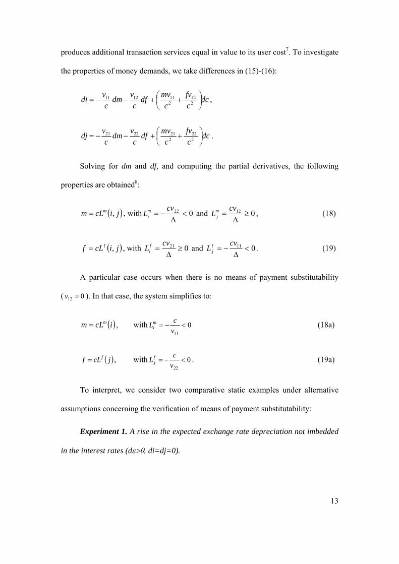
produces additional transaction services equal in value to its user cost7. To investigate

the properties of money demands, we take differences in (15)-(16):

dccfv

cmvdf

cvdm

cvdi ⎟

⎠⎞

⎜⎝⎛ ++−−= 2

122111211 ,

dccfv

cmvdf

cvdm

cvdj ⎟

⎠⎞

⎜⎝⎛ ++−−= 2

222212221 .

Solving for dm and df, and computing the partial derivatives, the following

properties are obtained8:

( )jicLm m ,= , with 022 <Δ

−=cvLm

i and 012 ≥Δ

=cvLm

j , (18)

( )jicLf f ,= , with 021 ≥Δ

=cvLf

i and 011 <Δ

−=cvLf

j . (19)

A particular case occurs when there is no means of payment substitutability

( 012 =v ). In that case, the system simplifies to:

( )icLm m= , with 011

<−=vcLm

i (18a)

( )jcLf f= , with 022

<−=vcLf

j . (19a)

To interpret, we consider two comparative static examples under alternative

assumptions concerning the verification of means of payment substitutability:

Experiment 1. A rise in the expected exchange rate depreciation not imbedded

in the interest rates (dε>0, di=dj=0).

14

According to (17), this causes an increase in the optimal proportion of assets

(money and bonds) denominated in foreign currency (AS), for speculative reasons.

Since the user costs of domestic and foreign money remain constant, however, this

change does not impact on individual money demands. This result holds

irrespectively of whether the two monies compete in the same commodity domain

( 012 >v ) or not ( 012 =v ).

Experiment 2. A rise in expected exchange rate depreciation accompanied by a

domestic interest rate rise, so that the expected return differential remains unchanged

(dε= di >0, dj=0).

According to equation (17), in this case the optimal proportion of assets

denominated in foreign currency (AS) remains unchanged. However, since the user

cost of the domestic money rises, the consumer will optimally reduce its demand for

domestic money. The remaining effects depend on whether there is means of payment

substitutability or not: in case 012 =v , then the adjustment involves only domestic

assets. In order to keep the denomination structure of the portfolio (AS) unchanged,

the decline in domestic money holdings is built up through purchases of domestic

bonds. The demand for domestic money (18a) is the same as in a closed economy9. If

instead 012 >v , then, as the demand for domestic money declines, the marginal

contribution of foreign money to the reduction of transactions costs ( 2v− ) rises.

According to (16), this leads to an increase in the demand for foreign money, for

transaction purposes. In order to keep the currency composition of the overall

portfolio unchanged, the consumer offsets the move by selling dollar-denominated

bonds. In this case, there is CS but the level of AS remains unchanged.

15

These experiments illustrate the Thomas (1985) separation result: on the one

hand, the consumer selects his currency holdings, based on each money's transaction

services and associated user cost. On the other hand, she borrows or lends to achieve

the desired level of AS. An optimal currency hedge is created and the denomination

structure of the individual portfolio is independent of money holdings.

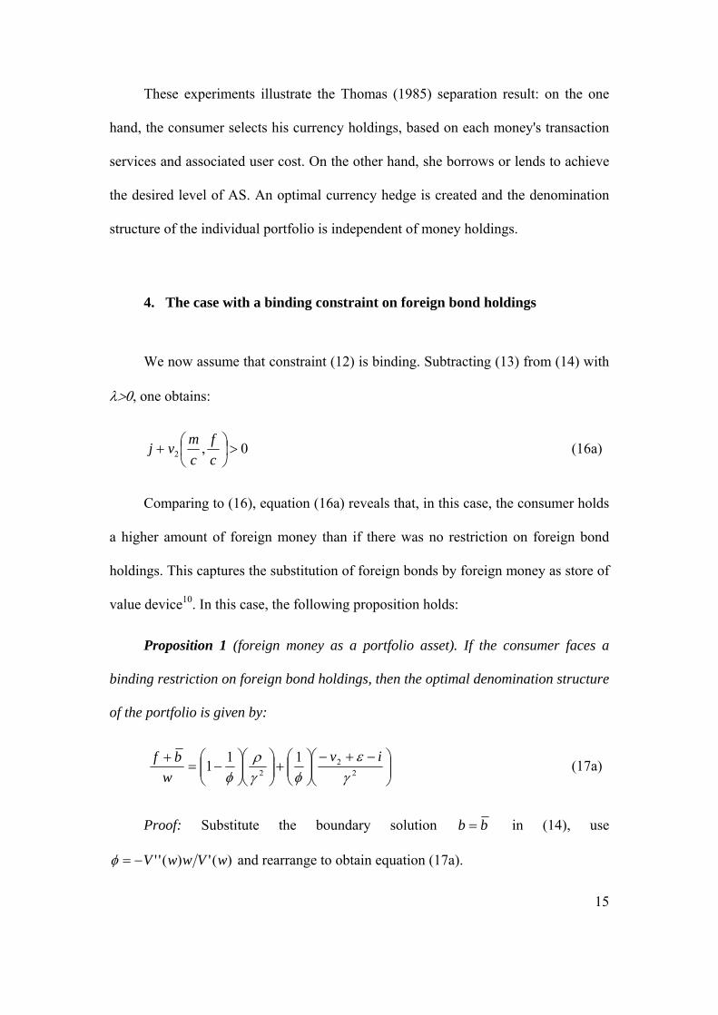
4. The case with a binding constraint on foreign bond holdings

We now assume that constraint (12) is binding. Subtracting (13) from (14) with

λ>0, one obtains:

0,2 >⎟⎠⎞

⎜⎝⎛+

cf

cmvj (16a)

Comparing to (16), equation (16a) reveals that, in this case, the consumer holds

a higher amount of foreign money than if there was no restriction on foreign bond

holdings. This captures the substitution of foreign bonds by foreign money as store of

value device10. In this case, the following proposition holds:

Proposition 1 (foreign money as a portfolio asset). If the consumer faces a

binding restriction on foreign bond holdings, then the optimal denomination structure

of the portfolio is given by:

⎟⎟⎠

⎞⎜⎜⎝

⎛ −+−⎟⎟⎠

⎞⎜⎜⎝

⎛+⎟⎟

⎠

⎞⎜⎜⎝

⎛⎟⎟⎠

⎞⎜⎜⎝

⎛−=

+2

22

111γ

εφγ

ρφ

ivw

bf (17a)

Proof: Substitute the boundary solution bb = in (14), use

)(')('' wVwwV−=φ and rearrange to obtain equation (17a).

16

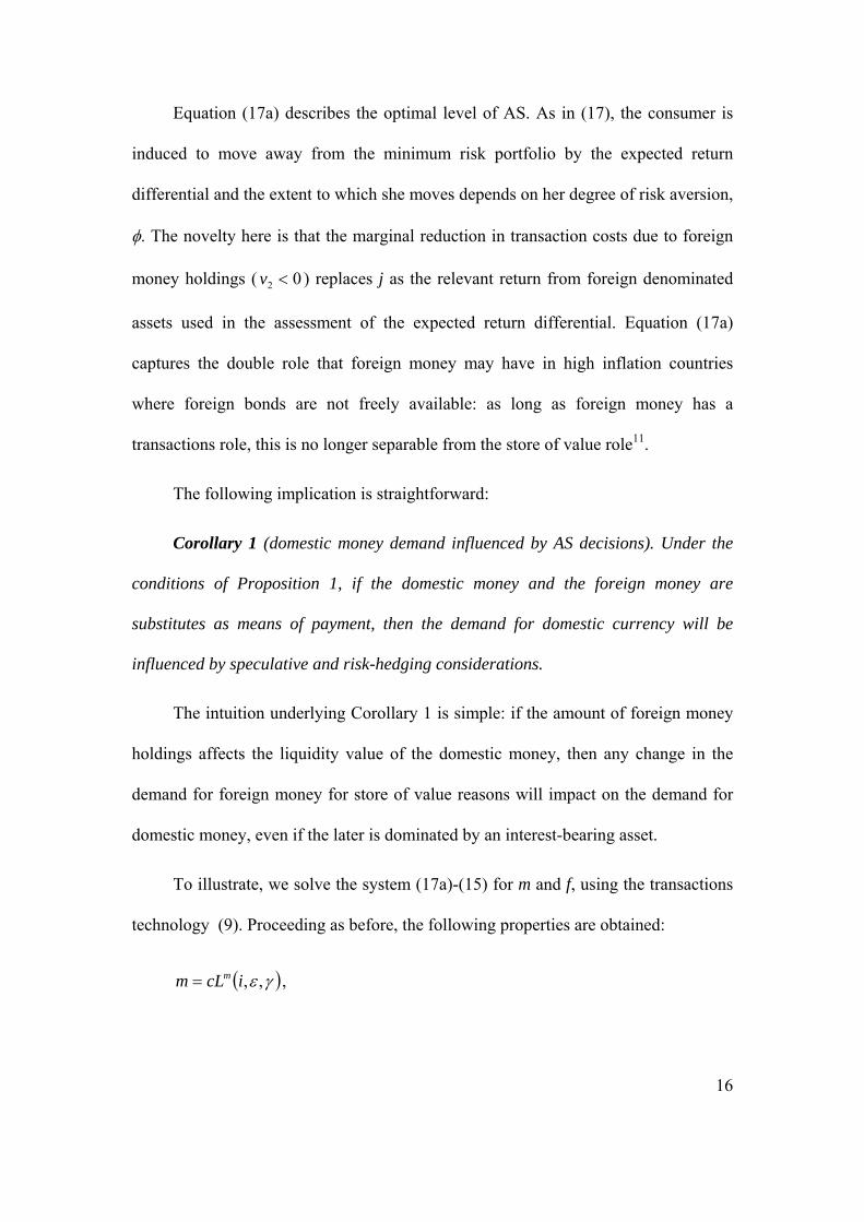
Equation (17a) describes the optimal level of AS. As in (17), the consumer is

induced to move away from the minimum risk portfolio by the expected return

differential and the extent to which she moves depends on her degree of risk aversion,

φ. The novelty here is that the marginal reduction in transaction costs due to foreign

money holdings ( 02 <v ) replaces j as the relevant return from foreign denominated

assets used in the assessment of the expected return differential. Equation (17a)

captures the double role that foreign money may have in high inflation countries

where foreign bonds are not freely available: as long as foreign money has a

transactions role, this is no longer separable from the store of value role11.

The following implication is straightforward:

Corollary 1 (domestic money demand influenced by AS decisions). Under the

conditions of Proposition 1, if the domestic money and the foreign money are

substitutes as means of payment, then the demand for domestic currency will be

influenced by speculative and risk-hedging considerations.

The intuition underlying Corollary 1 is simple: if the amount of foreign money

holdings affects the liquidity value of the domestic money, then any change in the

demand for foreign money for store of value reasons will impact on the demand for

domestic money, even if the later is dominated by an interest-bearing asset.

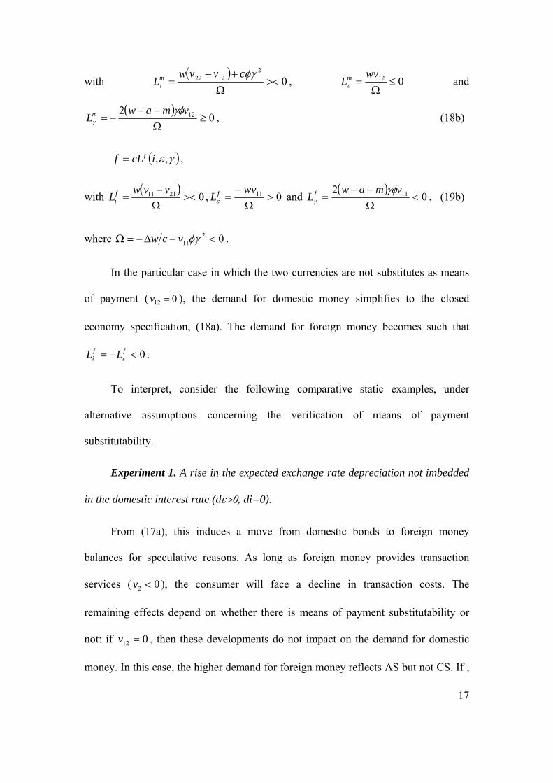
To illustrate, we solve the system (17a)-(15) for m and f, using the transactions

technology (9). Proceeding as before, the following properties are obtained:

( )γε ,,icLm m= ,

17

with ( )

02

1222 ><Ω

+−=

φγcvvwLm

i , 012 ≤Ω

=wv

Lmε and

( )0

2 12 ≥Ω−−

−=vmaw

Lm γφγ , (18b)

( )γε ,,icLf f= ,

with ( ) 02111 ><Ω−

=vvwLf

i , 011 >Ω

−=

wvLf

ε and ( )

02 11 <

Ω−−

=vmaw

Lf γφγ , (19b)

where 0211 <−Δ−=Ω φγvcw .

In the particular case in which the two currencies are not substitutes as means

of payment ( 012 =v ), the demand for domestic money simplifies to the closed

economy specification, (18a). The demand for foreign money becomes such that

0<−= ffi LL ε .

To interpret, consider the following comparative static examples, under

alternative assumptions concerning the verification of means of payment

substitutability.

Experiment 1. A rise in the expected exchange rate depreciation not imbedded

in the domestic interest rate (dε>0, di=0).

From (17a), this induces a move from domestic bonds to foreign money

balances for speculative reasons. As long as foreign money provides transaction

services ( 02 <v ), the consumer will face a decline in transaction costs. The

remaining effects depend on whether there is means of payment substitutability or

not: if 012 =v , then these developments do not impact on the demand for domestic

money. In this case, the higher demand for foreign money reflects AS but not CS. If ,

18

however, 012 >v , then the increased holdings of foreign money impact negatively on

the marginal contribution of domestic money to the reduction of transactions costs.

Thus, the demand for domestic money declines, as it is replaced by foreign money in

transactions. This second case illustrates how a pure speculative movement, rising the

demand for foreign money, is transmitted, through CS, to the demand for domestic

money.

Experiment 2. A rise in expected exchange rate depreciation embedded in the

domestic interest rate (dε= di >0).

From (17a), the optimal proportion of assets denominated in each currency does

not change for pure speculative reasons. However, from (15), the rise in the user cost

of the domestic money leads agents to reduce its demand. This, in turn, may or may

not impact on the level of AS: in case 012 =v , then the decline in the demand for

domestic money is built through purchases of domestic bonds only (just as in a closed

economy). In this case, the demand for foreign money remains unchanged and so will

the level of AS. If, however, 012 >v , then the decline in domestic money holdings

impacts positively on the marginal productivity of foreign money to the reduction of

transactions costs so that its demand rises for transaction purposes. This is a pure CS

effect that, notwithstanding, goes along with the level of AS.

It is important to observe that the signs of the partial derivatives with respect to

the domestic interest rate in (18b) and (19b) are uncertain. To understand this,

consider a third experiment, in which the domestic interest rate rises alone:

Experiment 3. A rise in the domestic interest rate not accompanied by the

expected exchange rate depreciation (di>0, dε=0).

19

From (17a), this induces a move from foreign money balances to domestic

bonds for speculative reasons. On the other hand, from (15), the rise in the user cost

of the domestic money leads agents to reduce its demand. Then: if 012 =v , there are

no transmission effects from one money market to the other. In this case, both the

decline in the demand for domestic money and the move out of foreign money

balances are built through purchases of domestic bonds only (note that, with 012 =v ,

miL and f

iL are unequivocally negative). If 012 >v , then the fall in the demand for

money in each denomination impacts positively on the marginal productivity of the

other money, inducing offsetting CS effects, through which both money demands

rise. To obtain negative elasticities ( 0<miL and 0<f

iL ), it is sufficient to assume that

own effects dominate over CS effects (that is 12vvkk > , with k=1,2). Other results are

however consistent with 0>Δ , in equation (9). For example, with 111222 vvv >> , one

would obtain 0>miL and 0<f

iL .

5. Implications for empirical work

In the empirical literature on CS, some authors have investigated the presence

of CS by evaluating the statistical significance of a term capturing the expected

exchange rate depreciation in the demand for domestic money (Fasano-Filho, 1987,

Kamin and Ericsson, 2003). Such procedure was criticised by Cuddington (1983), in

the context of the Portfolio Balance Approach to CS. This approach treats money as a

simple asset without specifying any particular feature so as to make it distinguishable

from the other assets. Postulating gross substitutability between money and all other

20

assets, this leads to money demand functions that depend positively on income and

wealth and negatively on the return of each alternative asset. When the available

assets are: domestic money, foreign money, domestic bonds and foreign bonds, the

following functional form has been proposed:

( ) εαεαααα 43210 loglog +++++=⎟⎠⎞

⎜⎝⎛ jiy

PM , (20)

with α1>0, α2<0, α3<0 and α4<0. The term α3 captures substitutability between the

domestic money and the foreign bond, and the term α4 captures substitutability

between the domestic money and the foreign money. Since the demand for domestic

money depends negatively on the expected exchange rate depreciation, both through

substitutability vis-à-vis the foreign money and substitutability vis-à-vis the foreign

bond, followers of the PBM have claimed that CS and capital mobility are

statistically indistinguishable. Moreover, in light of that approach, it has been argued

that the specification of a CS motive in the money demand does not constitute a

qualitative difference relative to a specification where either CS is ruled out or where

foreign monetary and non-monetary assets are implicitly lumped together

(Cuddington, 1983).

The Portfolio Balance Approach has two main shortcomings. First, as noted by

Branson and Henderson (1985), gross substitutability is not always consistent with

individual optimisation. Second, the model does not explain why money is held when

dominated by interest-bearing assets. A closer scrutiny of the properties of the money

demand in light of firmer microeconomic foundations was made by Thomas (1985),

for the case with complete bond markets. As shown in Section 3, in this case, there is

21

no demand for money as a “portfolio asset”. From equations (18) and (18a), a

possible specification to test for the presence of CS in this context is to investigate the

sign and the significance of β3 in:

jiyPM

3210 loglog ββββ +++=⎟⎠⎞

⎜⎝⎛ (21)

where β1>0, β2<0 and β3>0.

The Thomas model shall be seen as the centrepiece to test the CS hypothesis in

countries with developed financial markets. Not surprisingly, this model has been

used to test the presence of currency substitution among major currencies (Bergstrand

and Bundt, 1990, Mizen and Pentecost, 1994, Lebre de Freitas, 2006). Sahay and

Végh (1996) used the same model to discuss the case of high inflation countries

where bank deposits denominated in foreign currency are available, playing the role

of the missing bond. The Thomas model is less suitable, however, to describe the

phenomenon of CS in countries where consumers have no free access to interest-

bearing foreign assets. As pointed out by Cuddington (1989), in that case, one expects

the demand for foreign money to have a store of value role in addition to the eventual

means of payment role.

The results obtained in Section 4 give support to the Cuddington (1989, pp.

269) claim that, when foreign bonds are not freely available, the demand for foreign

money should reflect “a portfolio component”. They also imply that, in case the two

monies are substitutes as means of payment, the demand for domestic money will be

influenced by AS decisions. However, our findings do not give support to an

empirical test based on equation (20). Alternatively, equation (18b) suggests that a

22

valid test for the presence of CS in countries with imperfect capital mobility is to

access the sign and the significance of δ3 and δ4 in:

γδεδδδδ 43210 loglog ++++=⎟⎠⎞

⎜⎝⎛ iy

PM . (22)

where δ1>0, δ2 ><0, δ3<0 and δ4>0. Note that a similar exercise based on the

demand for foreign money (19b) does not necessarily reveal the presence of CS.

It may be argued that, under uncovered interest rate parity, the choice of the

particular model to be estimated is less relevant. This does not change, however, the

main result of this paper: irrespective of the degree of capital mobility, only in case of

CS will the demand for domestic money depart from the closed economy

specification (18a). Thus, the CS hypothesis may be investigated, without ambiguity

regarding the identification of the relevant effect.

6. Empirical application

In this section, an empirical test based on the theoretical model presented above

is implemented for six Latin American countries that experimented with restrictions

on capital flows for long periods of time. The focus on Latin America is motivated by

extensive background work reporting the presence of CS in the region (see, for

example, Calvo and Végh 1992, Guidotti and Rodriguez 1992, Savastano 1996, and

Kamin and Ericsson 2003) and also because of data availability12.

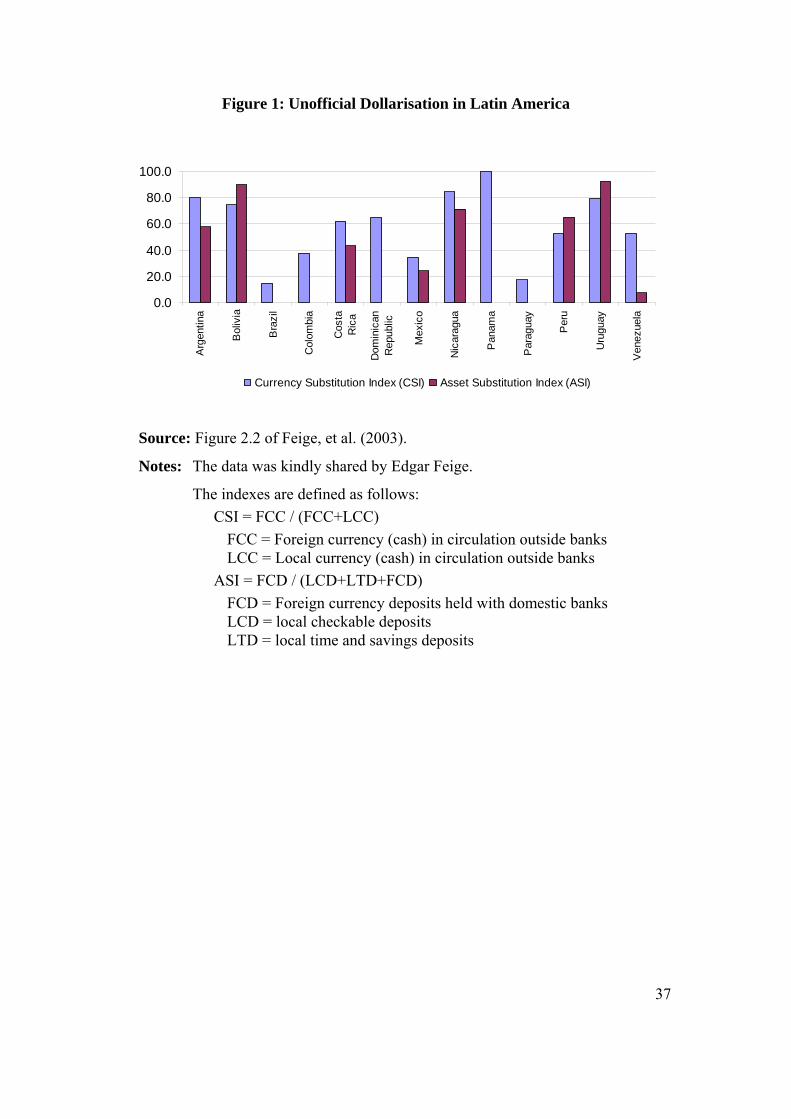
The departure point for the construction of the sample is the data on “unofficial

dollarisation”, collected by Feige, et al. (2003). These authors computed a “Currency

23

Substitution Index”, defined as the proportion of monetary assets outside banks that is

denominated in foreign currency. The estimates are based on reported shipments of

monetary assets denominated in U.S. dollars from the U.S. to different destinations.

The authors also computed an “Asset Substitution Index”, given by the ratio of

residents’ bank deposits denominated in foreign currency to total bank deposits.

Figure 1 shows the corresponding figures for 1997/98 for thirteen Latin American

countries.

-- Insert Figure 1 about here --

It should be noted that none of these measures corresponds to our definitions of

CS and AS. On the one hand, as long as foreign money may be held for store of value

reasons, the first measure does not necessarily indicate the extent to which it is

replacing domestic money as a vehicle for transactions. On the other hand, the

proposed index of AS does not measure the proportion of assets that are denominated

in foreign currency. Still, the latter may be suggestive of the extent to which foreign

banknotes are dominated by interest-bearing assets. Since our aim is to test for CS in

a context where foreign bank notes have a significant store of value role, our sample

is restricted to those countries in Figure 1 with a zero or very low “Asset Substitution

Index”. These are: Brazil, Colombia, the Dominican Republic, Paraguay and

Venezuela (Panama is not included because it is officially dollarised). To this group,

we add Chile because this country had high inflation rates in the 1970s and 1980s,

applied capital controls for a long period of time, and had relatively low financial

dollarization.13

24

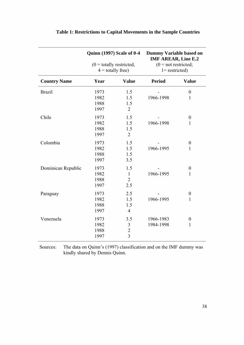
In order to restrict the analysis to periods with high restrictions on capital flows,

we use Quinn’s (1997) 0 to 4 measure of capital controls’ intensity and also the IMF

Annual Report on Exchange Arrangements and Exchange Restrictions (AREAR),

which are reported in Table 1 for the six countries under study. According to the

table, with the exception of Venezuela, all countries in this sample had capital

controls in place for around 30 years. Using quarterly data, this allows for a very

reasonable number of observations. Because of data availability, the sample period

starts in 1970, except for Chile, for which interest rate data is available only after

1977, and for Venezuela, which applied capital/exchange controls only after 198414.

-- Insert Table 1 about here --

The model to be estimated does not impose a priori the functional form (22). It

is instead general enough to account also for models (20) and (21). With this

procedure we allow the data to select the appropriate model. In order to account for

eventual non-stationarity of real money15 and of independent variables, we employ

the Stock and Watson (1993) Dynamic OLS methodology, according to which one

regresses the dependent variable with the contemporaneous levels of the explanatory

variables, leads and lags of their first differences, and a constant. Since real money is

not seasonally adjusted, we also include quarterly dummy variables. Finally, the first

lag of real money is included to account for autocorrelation. The equation to be

estimated is the following 16:

ti

itii

itii

itii

itii

iti

tsssttttt

t

vjiY

PMaqaajaiaYaa

PM

∑∑∑∑∑

∑

−=−

−=−+

−=−

−=−

−=−

−=+

+Δ+Δ+Δ+Δ+Δ+

⎟⎠⎞

⎜⎝⎛+++++++=⎟

⎠⎞

⎜⎝⎛

3

3

3

31

3

3

3

3

3

3

16

3

15143210

log

logloglog

γϕεφδβα

φγε

(23)

25

where M/P is real money (Money, IMF-IFS, line 34, divided by the CPI, IMF-IFS,

line 64), Y is real GDP (nominal GDP, IMF-IFS, line 98B, divided by the CPI, IMF-

IFS, line 64), i is the domestic interest rate (IMF-IFS, line 60B, 60L or 60 – according

to availability), j is the U.S. treasury bill rate (IMF-IFS, line 60c), ε is the one quarter

ahead expected exchange rate depreciation (for which we use three alternative

proxies as explained below), γ is the standard deviation of the exchange rate (IMF-

IFS, line RF) computed over the last one to three years, depending on which

maximizes the Schwartz Bayesian Information Criterion (SBIC), qi are the quarterly

dummy variables and u is the error term17. Although we start with a model that

includes all leads and lags of the explanatory variables up to order 3, the SBIC is used

to obtain a more parsimonious model.

Three alternative proxies for the one quarter ahead expected exchange rate

depreciation are tested: the inflation differential relative to the United States (based

on the relative version of the Purchasing Power Parity), the current quarter

depreciation rate (“myopic” expectations) and a forecast based on information

available at the time expectations were formed (rational expectations). The last case

is estimated using Two Stage Least Squares (2SLS), with the choice of the

instruments for the expected exchange rate depreciation driven by the results of the

first stage estimations18.

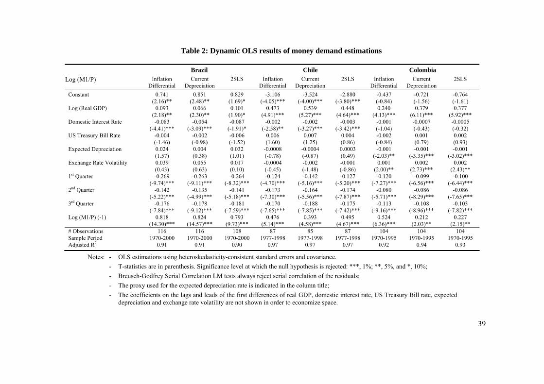
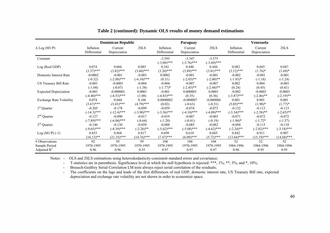
Table 2 shows the estimation results for each one of the six countries selected,

using the three alternative proxies for the expected exchange rate depreciation. In

general, the coefficients on GDP and on the domestic interest rate are statistically

significant, and with the conventional signs. As expected in a sample restricted to

26

periods with capital controls, the US Treasury Bill rate is seldom statistically

significant. The only exception is Paraguay, for which it has the wrong sign.

-- Insert Table 2 about here --

As far as the verification of the CS hypothesis is concerned, the results point to

two distinct cases: firstly, in Brazil and Chile, no other variable apart from those

appearing in a standard (closed economy) specification of the money demand was

found to be statistically significant. According to our theoretical model, this is

suggestive of absence of CS. Secondly, in Colombia, the Dominican Republic and

Venezuela, both the expected depreciation term and the volatility term are in general

statistically significant and with the respective signs according to model (22) (in the

case of the Dominican Republic, results for the 2SLS are less conclusive, but

probably this is due to misspecification of the forecasting model). This is suggestive

of the presence of CS. The case of Paraguay reveals some ambiguity, because the

exchange rate depreciation is statistically significant in one equation but no other

result points to CS (also note that the estimated coefficient for the Treasury Bill rate

has the wrong sign).19

The findings for Brazil and Chile are consistent with the general assertion that

these two countries have been an exception in the context of Latin America: despite

the several episodes of high inflation in these two countries, it appears that they did

not translate into a significant replacement of their respective monies by the U.S.

Dollar as vehicle for transactions (see, for example, Savastano 1996, p. 225). For the

remaining countries, one would like to confront the results with an effective measure

27

of the extent to which foreign money has been used as means of payment. To the best

of our knowledge, however, no such measure exists.

Comparing the estimation results with the data displayed in Figure 1, we

observe that the countries with higher “Currency Substitution Index” are those for

which evidence of CS was found. Obviously, this does not validate the procedure of

assessing the extent of CS by estimating the stock of foreign money balances held by

the public. But it is consistent with the view that CS is more likely when a

considerable demand for foreign money as store of value already exists (this pattern

is suggested, for example, in Calvo and Végh, 1992). In light of that interpretation, in

Brazil and Chile, where indexed bonds denominated in domestic currency became

popular, the demand for foreign money as store of value never reached such a critical

level so as to induce its acceptability as means of payment20.

7. Conclusions

This paper extends the Thomas (1985) dynamic optimising model of money

demand and currency substitution to the case in which the individual faces a binding

restriction on foreign bond holdings. In this case, foreign bank notes may have a store

of value role in addition to the eventual means of payment role. We show that means

of payment substitutability acts as a channel through which risk-hedging and

speculative decisions involving the demand for foreign money impact on the demand

for domestic money. Moreover, we show that only in case of currency substitution

will the demand for domestic money depart from the closed economy specification.

The results contradict Cuddington (1983, 1989)’s influential claim that the

28

significance of an expected depreciation term in the demand for domestic money does

not provide a valid test for the presence of CS. This implication is convenient for

empirical purposes: if the CS hypothesis can be assessed by estimating a demand

function for domestic money, the problem of disentangling whether foreign money is

merely held for store of value purposes or is indeed replacing domestic money as

vehicle for transactions is circumvented.

Applying the test to six Latin American countries that imposed restrictions on

capital flows for long periods of time, we found evidence of CS in Colombia, the

Dominican Republic and Venezuela, ambiguous evidence in Paraguay and no

evidence at all in Brazil and Chile. Comparing with existing estimates for the amount

of foreign money holdings in these countries, we find consistency with the view that

CS is more likely to occur when a considerable demand for foreign money for store

of value reasons already exists.

References

Agénor, Pierre and Mohsin Khan (1996) ‘Foreign Currency Deposits and the demand

for money in developing countries,’ Journal of Development Economics 50,

101-118

Alami, Tarik (2004) ‘Counter-argumentations on a comment of Tarik H. Alami's

Currency Substitution vs. Dollarization: a portfolio balance model, Journal of

Policy Modeling 23, 473-479,’ Journal of Policy Modeling 26, 117-122

29

Bergstrand, Jeffrey and Thomas Bundt (1990) ‘Currency substitution and monetary

autonomy: the foreign demand for US deposits,’ Journal of International

Money and Finance 9, 325-34

Branson, William and Dale Henderson (1985) ‘The specification and influence of

asset markets,’ in: Handbook of International Economics, Vol. II, ed. R. W.

Jones and P. B. Kenen (Amsterdam: North Holland)

Calvo, Guillermo and Carlos Rodríguez (1977) ‘A model of exchange rate

determination under currency substitution and rational expectations,’ Journal of

Political Economy 85, 617-24

Calvo, Guillermo and Carlos Végh (1992) ‘Currency substitution in developing

countries: An introduction,’ Revista de Análisis Económico, 7, 3-28

Chang, Roberto (1994) ‘Endogenous currency substitution and inflationary finance,

and welfare,’ Journal of Money, Credit and Banking 26, 903-916

Cuddington, John (1983) ‘Currency Substitutability, Capital Mobility and Money

Demand,’ Journal of International Money and Finance 2, 111-133

Cuddington, John (1989) ‘Review of ‘Currency Substitution: Theory and Evidence

from Latin America’ by V.A. Canto and G. Nickelburg, Journal of Money,

Credit and Banking 21, 267-271

Engineer, Merwan (2000) ‘Currency transaction costs and competing fiat currencies,’

Journal of International Economics 52, 113-136

Fasano-Filho, Ugo (1987) Currency substitution and liberalization: the case of

Argentina (Aldeshot: Gower Publishing Co.)

30

Feige, Edgar, Michael Faulend, Velimir Sonje, and Vedran Sosic (2003) ‘Unofficial

Dollarization in Latin America: Currency Substitution, Network Externalities,

and Irreversibility,’ in The Dollarization Debate, ed. D. Salvatore, J. Dean, and

T. Willett (Oxford: Oxford University Press), 46-71

Giovannini, Aalberto and Bart Turtelboom (1994) ‘Currency Substitution,’ in The

Handbook of International Macroeconomics, ed. Frederick Van Der Ploeg

(Oxford: Blackwell), 390-436

Guidotti, Pablo and Carlos Rodriguez (1992) ‘Dollarisation in Latin America:

Gresham's Law in reverse?’ International Monetary Fund Staff Papers 39 (3),

518-544

Imrohoroglu, Selahattin (1994) ‘GMM Estimates of Currency Substitution between

the Canadian Dollar and the US Dollar,’ Journal of Money, Credit and

Banking, 26 (3), 792-807

Kamin, Steven and Neil Ericsson (2003) ‘Dollarisation in Post-hyperinflationary

Argentina,’ Journal of International Money and Finance 22, 185-211

Kareken, John and Neil Wallace (1981) ‘On the indeterminacy of equilibrium

exchange rates,’ Quarterly Journal of Economics 96, 207-22

Krueger, Russel and Jiming Ha (1996) ‘Measurement of cocirculation of currencies,’

in The Macroeconomics of International Currencies: Theory, Policy and

Evidence, ed. P. Mizen and E. Pentecost (Cheltenham: Edward Elgar), 60-76.

Krugman, Paul (1984) ‘The international role of the dollar: theory and prospect,’ in

Exchange Rate in Theory and Practice, ed. J. F. Bilson and R.C. Martson

(Chicago: University of Chicago Press)

31

Lebre de Freitas, Miguel (2004) ‘The dynamics of Inflation and Currency

Substitution in a Small Open Economy,’ Journal of International Money and

Finance 23 (1), 133-142

Lebre de Freitas, Miguel (2006) ‘Currency Substitution and Money Demand in

Euroland,’ forthcoming in Atlantic Economic Journal, 34 (3), September.

Levy-Yeyati, Eduardo (2006) ‘Financial Dollarization: Evaluating the

Consequences,’ forthcoming in Economic Policy.

Miles, Marc (1978) ‘Currency Substitution, Flexible Exchange Rates, and Monetary

Independence,’ American Economic Review 68, 428-436

Mizen, Paul and Eric Pentecost (1994) ‘Evaluating the Empirical Evidence for

Currency Substitution: A Case Study of the Demand for Sterling in Europe,’

The Economic Journal 104 (426), 1057-1069

Quinn, Dennis (1997) ‘The Correlates of Change in International Financial

Regulation,’ American Political Science Review 91 (September), 531-551

Rheinhart, Carmen and Kenneth Rogoff (2004) ‘The Modern History of Exchange

Rate Arrangements: A Reinterpretation,’ Quarterly Journal of Economics,

CXIX(1), 1-48

Rojas-Suárez, Liliana (1992) ‘Currency substitution and inflation in Peru,’ Revista de

Análisis Económico 7(1), 151-176

Rogers, John (1990) ‘Foreign Inflation Transmission under Flexible Exchange Rates

and Currency Substitution,’ Journal of Money, Credit and Banking 22 (9), 195-

208

32

Sahay, Ratna and Carlos Végh (1996) ‘Dollarisation in Transition Economies,

Evidence and Policy Implications,’ in The Macroeconomics of International

Currencies: Theory, Policy and Evidence, ed. P. Mizen and E. Pentecost

(Cheltenham: Edward Elgar), 193-224

Savastano, Miguel (1996) ‘Dollarisation in Latin America: recent evidence and

policy issues,’ in The Macroeconomics of International Currencies: Theory,

Policy and Evidence, ed. P. Mizen and E. Pentecost (Cheltenham: Edward

Elgar), 193-224

Smith, Constance (1995) ‘Substitution, Income and Intertemporal Effects in

Currency-Substitution Models,’ Review of International Economics 3 (1), 53-59

Stock, James and Mark Watson (1993) ‘A simple estimator of cointegrating vectors

in higher order integrated systems,’ Econometrica 61(4), 783-820

Sturzenegger, Federico (1997) ‘Understanding the welfare implications of currency

substitution,’ Journal of Economic Dynamics and Control 21, 391-416

Thomas, Lee (1985) ‘Portfolio Theory and Currency Substitution,’ Journal of Money,

Credit and Banking 17 (2), 347-357

Uribe, Martín (1997) ‘Hysteresis in a simple model of currency substitution,’ Journal

of Monetary Economics 40, 185-202

Végh, Carlos (1989) ‘The optimal inflation tax in the presence of currency

substitution,’ Journal of Monetary Economics 24, 139-146

Whited, Hsin-hui (2004) ‘Comment on Currency Substitution vs. Dollarization: a

portfolio balance model,’ Journal of Policy Modelling 26, 113-116

33

Lead Footnote:

Both authors are members of NIPE. Earlier versions of this paper were presented in the 2004 Latin

American meeting of the Econometric Society and in the 2003 meeting of The Latin American and

Caribbean Economic Association. The authors acknowledge Richard C. Barnett and two anonymous

referees for helpful comments, and Edgar Feige and Dennis Quinn for sharing very useful data.

1 The terminology follows Sahay and Végh (1996). Different meanings for the terms “currency

substitution” and “dollarisation” are however common in the literature. For a survey, see Giovannini

and Turtelbomm (1994).

2 Recent theories have related imperfect means of payment substitutability to the existence of

transaction costs on the use of foreign currency. This includes Guidotti and Rodriguez (1992), Chang

(1994), Uribe (1997), Sturzenegger (1997) and Engineer (2000).

3 Extending the model to the presence of a safe asset leads to a currency substitution problem that is

embedded in the optimal portfolio choice between the safe asset and the risky assets (the Merton

problem). This extension is available from the authors upon request.

4 With such specification, asset demands will be neutral in respect to the domestic inflation rate.

Thomas (1985) deflated domestic assets by the domestic price level and foreign assets by the foreign

price level, and introduced uncertainty in the foreign inflation rate instead of on the exchange rate.

Although the two specifications are equivalent for the purposes of our discussion, the one followed in

this paper looks more useful to describe the case in which a foreign money can be used along with the

domestic money as vehicle for transactions that take place in the domestic economy.

5 An alternative specification would assume that money enters in the utility function. The two

approaches become functionally equivalent if the utility function is weakly separable, as happens to be

the case in most of the CS literature. For a stochastic model with money in utility, currency

substitution and complete bond markets, see Smith (1995).

34

6 As shown by Sahay and Végh (1996), and briefly reviewed in Section 3, in the case with complete

bond markets, these conditions are sufficient to obtain sensible money demand functions. In Section

4, we show that, when bonds denominated in foreign currency are not freely available, further

assumptions are needed to obtain unambiguous interest-rate elasticities.

7 Conditions similar to (15) and (16) were first obtained by Miles (1978), in the context of the two-step

monetary model of CS. In that approach, CS decisions are postulated to be separate from the choice

among non-monetary assets. The proof that separability of CS decisions holds in the dynamic

optimising model with complete bond markets is from Thomas (1985).

8 Equations (18) and (19) are not in the reduced form because changes in the interest rates also impact

on money demands through wealth effects. However, the aim of the exercise is to learn about money

velocities, so as to obtain testable money demand functions.

9 In the extreme case in which dollar bank notes provided no transaction services at all (that is, when

0222 == vv ), then condition (16) would not hold in equality and the optimal demand for dollars

would be zero. The demand for pesos, however, would still be as described by (18a). Note that, apart

from this extreme case, the rise in the domestic interest rate leads to an increase in the proportion of

money balances that is denominated in foreign currency, even in the absence of CS.

10 The model may also be solved considering a non-negative restriction on foreign bond holdings,

0≥b (that is, the individual is not allowed to borrow in foreign currency). When such restriction is

binding, the sign of the inequality in (16a) is reversed. This means that the use of foreign money for

transaction purposes (and the eventual level of CS) is constrained by the absence of hedging

opportunities in the bond market. Although interesting at the theoretical level, this case is at odds with

the observation that in high inflation countries, a large demand for foreign money is primarily held for

store of value reasons.

35

11 If the consumer had no access to domestic bonds either, one would obtain an optimal portfolio rule

similar to (17a), except that i would be replaced by - 1v in the interest differential. Currency

substitution in a world without bonds was first discussed in the context of the monetary model by

Calvo and Rodrígues (1977), and is analysed in the context of the liquidity services model by Rojas-

Suarez (1992).

12 Although several African countries have experimented capital/exchange controls and CS, data

limitations are more serious in that region.

13 Levy-Yeyati’s (2006) data on financial dollarisation covers Chile from 1976 to 2001. On average,

during this period, foreign currency deposits in Chile where below 10 per cent of total deposits.

14 In the case of Venezuela, the dummy variable based on the IMF AREAR is equal to one from 1984

to 1998, meaning high restrictions on capital flows. Quinn (1997), in turn, assigns a grade of 3 in

1997, meaning very little restrictions. Taking into account the two sources, we decided to restrict the

period with capital/exchange controls in this country to 1984-1996.

15 Augmented Dickey-Fuller (ADF), Phillips-Perron (PP) and Kwiatkowski-Phillips-Schmidt-Shin

(KPSS) tests indicate that log(M/P) is stationary in Brazil, Chile and the Dominican Republic, and has

a unit root in Paraguay and Venezuela. Results for Colombia are mixed, as a PP test rejects the null

hypothesis of a unit root, but the ADF test does not, and the KPSS rejects the null hypothesis of

stationarity. Unit root tests are available from the authors upon request.

16 The constant term was excluded from estimations in the cases of the Dominican Republic and

Venezuela, as it was never statistically significant when included.

17 Whenever quarterly data on GDP was not available, it was estimated from annual data using the

frequency conversion option “cubic match last” of Eviews 5.0. The money market rate (line 60B) is

only available with a reasonable number of observations for Brazil and Paraguay. The time deposits

rate (line 60L) was used instead in the cases of Chile and Dominican Republic. In Colombia and

Venezuela, we used the discount rate (line 60). Since interest rate data starts in 1991 in the case of the

36

Dominican Republic, and in 1990 in the case of Paraguay, the previous values of these countries’

interest rate series were proxied by the 4-quarter change in the CPI (IMF-IFS, line 64X). Since Brazil

faced two hyperinflations during the sample period, it has much greater variance of prices, interest

rates and exchange rates than the other five countries. For that reason, in the estimations for Brazil, the

interest rate and the expected depreciation rate are used in logs, and the exchange rate volatility is

proxied by the coefficient of variation of the exchange rate (instead of the standard deviation).

18 The results for the first stage estimations are shown in the Appendix. We followed a general to

specific approach, in which, besides the explanatory variables of the base model, we include in the list

of instruments: the current and lagged depreciation rates, the current and lagged inflation differentials,

the current and lagged growth rates of monetary expansion, and the current and lagged percentage

differences between official and parallel exchange rates (data on the latter is from Rheinhart and

Rogoff, 2004). The variables that were not statistically significant were sequentially excluded until we

reached a parsimonious model that maximized the SBIC.

19 In order to control for an eventual Cagan effect in the money demand, the four-quarter change in the

CPI (the homologous inflation rate) was included in the model. This inclusion did not change the

results for the remaining explanatory variables nor our conclusions regarding the existence of

Currency Substitution in the six countries under analysis.

20 Uribe (1997) and Sturzenegger (1997) stress the role of network externalities in the use of money in

shaping the relationship between the aggregate demand for foreign money and its acceptability as

means of payment. In terms of our model, network externalities would be accounted for in a general

equilibrium set-up by making the transactions technology (9) depend on the aggregate stocks of

domestic and foreign monies. To the extent that the size of the network cannot be influenced by

individual decisions, however, the latter would be invariant in respect to that specification.

37

Figure 1: Unofficial Dollarisation in Latin America

0.0

20.0

40.0

60.0

80.0

100.0

Arg

entin

a

Bol

ivia

Bra

zil

Col

ombi

a

Cos

taR

ica

Dom

inic

anR

epub

lic

Mex

ico

Nic

arag

ua

Pan

ama

Par

agua

y

Per

u

Uru

guay

Ven

ezue

la

Currency Substitution Index (CSI) Asset Substitution Index (ASI)

Source: Figure 2.2 of Feige, et al. (2003).

Notes: The data was kindly shared by Edgar Feige.

The indexes are defined as follows: CSI = FCC / (FCC+LCC)

FCC = Foreign currency (cash) in circulation outside banks LCC = Local currency (cash) in circulation outside banks

ASI = FCD / (LCD+LTD+FCD) FCD = Foreign currency deposits held with domestic banks LCD = local checkable deposits LTD = local time and savings deposits

38

Table 1: Restrictions to Capital Movements in the Sample Countries

Quinn (1997) Scale of 0-4

(0 = totally restricted, 4 = totally free)

Dummy Variable based on IMF AREAR, Line E.2

(0 = not restricted; 1= restricted)

Country Name Year Value Period Value

Brazil 1973 1.5 - 0 1982 1.5 1966-1998 1 1988 1.5 1997 2

Chile 1973 1.5 - 0 1982 1.5 1966-1998 1 1988 1.5 1997 2

Colombia 1973 1.5 - 0 1982 1.5 1966-1995 1 1988 1.5 1997 3.5

Dominican Republic 1973 1.5 - 0 1982 1 1966-1995 1 1988 2 1997 2.5

Paraguay 1973 2.5 - 0 1982 1.5 1966-1995 1 1988 1.5 1997 4

Venezuela 1973 3.5 1966-1983 0 1982 3 1984-1998 1 1988 2 1997 3

Sources: The data on Quinn’s (1997) classification and on the IMF dummy was kindly shared by Dennis Quinn.

39

Table 2: Dynamic OLS results of money demand estimations

Brazil Chile Colombia Log (M1/P) Inflation

Differential Current

Depreciation 2SLS Inflation

Differential Current

Depreciation 2SLS Inflation

Differential Current

Depreciation 2SLS

Constant 0.741 (2.16)**

0.851 (2.48)**

0.829 (1.69)*

-3.106 (-4.05)***

-3.524 (-4.00)***

-2.880 (-3.80)***

-0.437 (-0.84)

-0.721 (-1.56)

-0.764 (-1.61)

Log (Real GDP) 0.093 (2.18)**

0.066 (2.30)**

0.101 (1.90)*

0.473 (4.91)***

0.539 (5.27)***

0.448 (4.64)***

0.240 (4.13)***

0.379 (6.11)***

0.377 (5.92)***

Domestic Interest Rate -0.083 (-4.41)***

-0.054 (-3.09)***

-0.087 (-1.91)*

-0.002 (-2.58)**

-0.002 (-3.27)***

-0.003 (-3.42)***

-0.001 (-1.04)

-0.0007 (-0.43)

-0.0005 (-0.32)

US Treasury Bill Rate -0.004 (-1.46)

-0.002 (-0.98)

-0.006 (-1.52)

0.006 (1.60)

0.007 (1.25)

0.004 (0.86)

-0.002 (-0.84)

0.001 (0.79)

0.002 (0.93)

Expected Depreciation 0.024 (1.57)

0.004 (0.38)

0.032 (1.01)

-0.0008 (-0.78)

-0.0004 (-0.87)

0.0003 (0.49)

-0.001 (-2.03)**

-0.001 (-3.35)***

-0.001 (-3.02)***

Exchange Rate Volatility 0.039 (0.43)

0.055 (0.63)

0.017 (0.10)

-0.0004 (-0.45)

-0.002 (-1.48)

-0.001 (-0.86)

0.001 (2.00)**

0.002 (2.73)***

0.002 (2.43)**

1st Quarter -0.269 (-9.74)***

-0.263 (-9.11)***

-0.264 (-8.32)***

-0.124 (-4.70)***

-0.142 (-5.16)***

-0.127 (-5.20)***

-0.120 (-7.27)***

-0.099 (-6.56)***

-0.100 (-6.44)***

2nd Quarter -0.142 (-5.22)***

-0.135 (-4.99)***

-0.141 (-5.18)***

-0.173 (-7.30)***

-0.164 (-5.56)***

-0.174 (-7.87)***

-0.080 (-5.71)***

-0.086 (-8.29)***

-0.086 (-7.65)***

3rd Quarter -0.176 (-7.84)***

-0.178 (-9.12)***

-0.181 (-7.59)***

-0.170 (-7.65)***

-0.188 (-7.85)***

-0.175 (-7.42)***

-0.113 (-9.16)***

-0.108 (-8.96)***

-0.103 (-7.82)***

Log (M1/P) (-1) 0.818 (14.30)***

0.824 (14.57)***

0.793 (9.73)***

0.476 (5.14)***

0.393 (4.58)***

0.495 (4.67)***

0.524 (6.36)***

0.212 (2.03)**

0.227 (2.15)**

# Observations 116 116 108 87 85 87 104 104 104 Sample Period 1970-2000 1970-2000 1970-2000 1977-1998 1977-1998 1977-1998 1970-1995 1970-1995 1970-1995 Adjusted R2 0.91 0.91 0.90 0.97 0.97 0.97 0.92 0.94 0.93

Notes: - OLS estimations using heteroskedasticity-consistent standard errors and covariance. - T-statistics are in parenthesis. Significance level at which the null hypothesis is rejected: ***, 1%; **, 5%, and *, 10%; - Breusch-Godfrey Serial Correlation LM tests always reject serial correlation of the residuals; - The proxy used for the expected depreciation rate is indicated in the column title; - The coefficients on the lags and leads of the first differences of real GDP, domestic interest rate, US Treasury Bill rate, expected

depreciation and exchange rate volatility are not shown in order to economize space.

40

Table 2 (continued): Dynamic OLS results of money demand estimations

Dominican Republic Paraguay Venezuela Δ Log (M1/P) Inflation

Differential Current

Depreciation 2SLS Inflation

Differential Current

Depreciation 2SLS Inflation

Differential Current

Depreciation 2SLS

Constant -2.593 (-3.08)***

-3.347 (-3.76)***

-3.375 (-3.69)***

Log (Real GDP) 0.074 (3.37)***

0.066 (3.82)***

0.085 (3.60)***

0.341 (3.20)***

0.440 (3.89)***

0.444 (3.81)***

0.082 (3.12)***

0.045 (1.76)*

0.047 (1.69)*

Domestic Interest Rate -0.0002 (-0.32)

-0.001 (-2.88)***

-0.003 (-6.10)***

0.0002 (0.31)

-0.001 (-2.03)**

-0.001 (-2.00)**

-0.002 (-1.93)*

-0.001 (-1.18)

-0.001 (-1.24)

US Treasury Bill Rate -0.001 (-1.04)

-0.0001 (-0.07)

-0.004 (-1.38)

-0.004 (-1.77)*

-0.007 (-2.45)**

-0.007 (-2.44)**

0.002 (0.24)

0.004 (0.45)

-0.003 (0.41)

Expected Depreciation -0.001 (-4.40)***

-0.000001 (-4.53)***

0.0001 (1.08)

-0.001 (-4.83)***

0.000003 (0.35)

0.0001 (0.36)

-0.002 (-3.87)***

-0.0003 (-2.46)**

-0.0003 (-2.19)**

Exchange Rate Volatility 0.074 (3.67)***

0.044 (3.43)***

0.106 (4.79)***

0.0000002 (0.02)

-0.000007 (-0.63)

-0.000006 (-0.51)

0.001 (5.05)***

0.001 (1.90)*

0.001 (1.77)*

1st Quarter -0.205 (-14.3)***

-0.178 (-12.4)***

-0.099 (-3.90)***

-0.059 (-3.56)***

-0.074 (-4.10)***

-0.073 (-4.09)***

-0.132 (-3.34)***

-0.113 (-2.58)**

-0.113 (-2.65)**

2nd Quarter -0.127 (-7.89)***

-0.090 (-6.04)***

-0.017 (-0.64)

-0.019 (-1.20)

-0.007 (-0.41)

-0.003 (-0.19)

-0.071 (-1.84)*

-0.072 (-1.72*

-0.072 (-1.57)

3rd Quarter -0.146 (-9.65)***

-0.130 (-8.39)***

-0.059 (-2.26)**

-0.088 (-5.62)***

-0.085 (-5.08)***

-0.082 (-4.62)***

-0.094 (-2.24)**

-0.115 (-2.82)***

-0.118 (-3.18)***

Log (M1/P) (-1) 0.853 (16.13)**

0.868 (21.35)***

0.817 (14.76)***

0.698 (7.47)***

0.610 (6.09)***

0.605 (5.72)***

0.842 (13.64)***

0.911 (15.19)***

0.907 (14.68)***

# Observations 92 95 95 104 104 104 52 52 52 Sample Period 1970-1995 1970-1995 1970-1995 1970-1995 1970-1995 1970-1995 1984-1996 1984-1996 1984-1996 Adjusted R2 0.96 0.96 0.55 0.97 0.97 0.97 0.96 0.95 0.95

Notes: - OLS and 2SLS estimations using heteroskedasticity-consistent standard errors and covariance; - T-statistics are in parenthesis. Significance level at which the null hypothesis is rejected: ***, 1%; **, 5%, and *, 10%; - Breusch-Godfrey Serial Correlation LM tests always reject serial correlation of the residuals; - The coefficients on the lags and leads of the first differences of real GDP, domestic interest rate, US Treasury Bill rate, expected

depreciation and exchange rate volatility are not shown in order to economize space.

41

Appendix- First stage results of the 2SLS estimations

Depreciation (+1) Brazil Chile Colombia Dominican Republic

Paraguay Venezuela

Constant -3.991 (-1.70)*

-235.55 (-0.71)

-47.813 (-0.64)

142.585 (0.81)

193.486 (0.44)

-15241.08 (-1.54)

Log (Real GDP) 0.158 (0.34)

48.290 (1.01)

3.077 (0.46)

-57.491 (-1.82)*

-24.634 (-0.45)

1322.368 (1.60)

National Interest Rate

0.403 (1.91)*

-0.373 (-0.60)

0.076 (0.30)

-0.326 (-1.42)

0.750 (1.12)

1.640 (0.88)

US Treasury Bill Rate

0.058 (2.66)***

-0.526 (-0.30)

0.437 (1.45)

0.716 (0.62)

-0.474 (-0.32)

51.822 (1.27)

Exchange Rate Volatility

0.639 (0.80)

-0.675 (-1.01)

-0.100 (-1.08)

1.308 (0.26)

-0.103 (-1.60)

-1.127 (-2.61)**

1st Quarter -0.366 (-2.22)**

5.334 (0.57)

0.082 (0.05)

25.657 (1.96)*

-7.355 (-0.42)

-27.527 (-0.51)

2nd Quarter -0.199 (-1.00)

24.688 (2.42)

-0.543 (-0.24)

23.726 (2.28)**

-25.134 (-1.99)**

-119.642 (-2.14)**

3rd Quarter -0.117 (-0.75)

6.796 (0.75)

1.874 (1.12)

25.315 (2.50)**

-19.070 (-1.98)*

-51.603 (-1.24)

Log (M1/P) (-1) 0.445 (1.34)

-74.869 (-1.33)

2.159 (0.11)

103.363 (2.35)**

40.568 (0.77)

58.638 (0.45)

Depreciation 0.388 (2.72)***

0.930 (6.78)***

-0.004 (-3.91)***

0.503 (3.81)***

0.752 (2.42)**

Depreciation (-1) -0.235 (-1.37)

-0.168 (-1.24)

-0.240 (-2.73)***

Inflation Differential

0.492 (3.35)***

0.331 (2.62)**

-2.160 (-1.45)

Inflation Differential (-1)

0.076 (2.34)**

% Difference between Official and Parallel

0.003 (1.66)*

0.164 (3.07)***

0.876 (1.92)*

Growth of M1 0.178 (1.87)*

# Observations 108 87 104 95 104 52 Sample Period 1970-

2000 1977-1998

1970-1995 1970-1995 1970-1995 1984-1996

Adjusted R2 0.88 0.46 0.73 0.32 0.20 0.23

Notes: - OLS estimations using heteroskedasticity-consistent standard errors and covariance; - T-statistics are in parenthesis. Significance level at which the null hypothesis

is rejected: ***, 1%; **, 5%, and *, 10%; - Breusch-Godfrey Serial Correlation LM tests always reject serial correlation

of the residuals; - The coefficients on the lags and leads of the first differences of real GDP,

domestic interest rate, US Treasury Bill rate expected depreciation and exchange rate volatility are not shown in order to economize space.