WP/05/13

Currency Crises in Developed and Emerging Market Economies:

A Comparative Empirical Treatment

Thomson Fontaine

© 2005 International Monetary Fund WP/05/13

IMF Working Paper

African Department

Currency Crises in Developed and Emerging Market Economies: A Comparative Empirical Treatment

Prepared by Thomson Fontaine1

Authorized for distribution by Godfrey Kalinga

January 2005

Abstract

This Working Paper should not be reported as representing the views of the IMF. The views expressed in this Working Paper are those of the author(s) and do not necessarily represent those of the IMF or IMF policy. Working Papers describe research in progress by the author(s) and are published to elicit comments and to further debate.

This paper takes a step in empirically testing the implications of a number of theoretical models that attempt to highlight the dynamics behind currency crises. By focusing on countries with broadly disparate economic and political arrangements, the study attempts to determine the extent to which these variables matter in affecting the probabilities of currency crises occurring. The empirical findings provide support for the view that, in general, a deterioration in economic fundamentals and the pursuit of lax monetary policy can contribute to currency crises. The experiences of several emerging market economies suggests that the sustainability of exchange rate policy depends both on adequate policy responses to the shocks to the economy and on the fragility of the economic, financial, and political system. JEL Classification Numbers: F31, F47 Keywords: Currency crises, financial crises, exchange rates Author(s) E-Mail Address: tfontaine@imf.org

1 I am grateful for the unfailing support of Dr. Myles Wallace of Clemson University in helping to guide the initial work on this paper. Special thanks also to Anupam Basu and my other IMF colleagues, especially Gian Maria Milesi-Ferretti and Jean Claude Nachega, for their very useful comments and suggestions.

- 2 -

Contents Page

I. Introduction ............................................................................................................................3

II. Historical Perspective............................................................................................................4

III. Discussion of the Literature .................................................................................................6

IV. Empirical Analysis...............................................................................................................8 A. Framework for Empirical Analysis...........................................................................8 B. Data and Empirical Measurement of Currency Crises............................................12 C. Estimation and Forecasting Ability.........................................................................16 D. Results Based on the Inclusion of the Macroeconomic and Political Risk Variables .................................................................................................................17 E. Results Based on a Comparison Between Developed and Emerging Market Economies...............................................................................................................23 F. Results Based on Estimation and Forecasting .........................................................23

V. Conclusion ..........................................................................................................................28 Tables 1. Logit Results of Estimated Coefficients Excluding Political Variable........................................................................................................................18 2. Logit Results Showing Marginal Effects Excluding Political Variable........................................................................................................................19 3. Logit Results of Estimated Coefficients Including Political Variable........................................................................................................................21 4. Logit Results Showing Marginal Effects Including Political Variable........................................................................................................................22 5. Logit Results of Marginal Effects for Differences in Slopes Excluding Political Variable........................................................................................24 6. Logit Results of Marginal Effects for Differences in Slopes Including Political Variable.........................................................................................26 7. Actual and Predicted Crises in and out of Sample for Developed Economies

(Prob=0.5)....................................................................................................................29 8. Actual and Predicted Crises in and out of Sample for Developed Economies

(Mean=0.38)................................................................................................................30 9. Actual and Predicted Crises in and out of Sample for Emerging Market Economies

(Prob = 0.5)..................................................................................................................31 10. Actual and Predicted Crises in and out of Sample for Emerging Market Economies

(Mean = 0.38)..............................................................................................................32 References................................................................................................................................35

- 3 -

I. INTRODUCTION

One of the most persuasive arguments in favor of a fixed exchange rate regime is that it imposes discipline on monetary and fiscal policies. Another compelling argument is that it alleviates problems of noncooperative decision making on the part of governments of interdependent economies. Fixing the exchange rate is therefore seen as a surrogate form of international policy coordination. These arguments, in effect, reinforce the belief that it is impossible to pursue a fixed exchange rate regime and monetary policies simultaneously. However, they do not take into consideration the speculative behavior of foreign exchange market participants, whose actions can have a decided impact on the value of a country's currency. Throughout the history of fixed exchange rates, both developed and emerging market economies have experienced repeated speculative currency attacks. Many of these attacks can occur unexpectedly, have real effects, and be purely self-fulfilling; moreover, they can sometimes be difficult to prevent. The far-reaching consequences of currency crises were dramatically highlighted with the 1997 Asian crisis, which ignited debate in academic and political circles about the causes and effects of such crises. This study presents a comparative empirical treatment of speculative attacks that may result in crises in developed and emerging market economies. The severity of such attacks is examined within the context of the varying economic conditions that characterize these economies. It is critically important to determine whether one group of countries routinely suffers greater adverse effects from a similar attack. Another area of focus is the relative importance of political influences in contributing to an explanation of the incidence of speculative attacks. Yet another aspect of the research establishes the existence of “contagion” within foreign exchange markets. The study uses a logit model that considers how various macroeconomic data and political events affect the probability of a crisis. It is based on data from 21 developed economies and 16 emerging market economies, with an emphasis on variables that are consistent with the literature on speculative attacks and currency crises.

The paper is organized as follows: Section II examines currency crises within a historical context; Section III discusses the work of various authors who have tried to explain currency crises; Section IV presents a detailed empirical analysis of the crisis phenomenon; and Section V presents the paper’s conclusions.

- 4 -

II. HISTORICAL PERSPECTIVE

The dramatic events that unfolded in east Asia in the summer of 1997 were only the latest in a series of currency crises that have occurred from time to time in various countries over the past two centuries. In a survey of the historical episodes of currency crises over that period, Bordo and Schwartz (1996) observed that currency crises occurred when internal economic conditions were incompatible with the external conditions set for the currency. However, the experiences of developing and developed economies were decidedly different.

Before World War II, crises in developed countries usually occurred during times of war, when it became apparent to market agents that, to pursue the war effort, governments would be forced to suspend the convertibility of their currencies. In peacetime, banking instability was mainly responsible. In contrast, developing countries often suspended convertibility when their currencies came under attack by market agents who perceived that their governments were pursuing lax financial policies.

Some famous historical examples of such crises are John Law’s operations (1716-20)2 and the Bank of England’s suspension of the gold standard in 1797 after its bullion reserves fell to just above £1 million (see O’Brien, 1967). During the U.S. dollar weakness of 1894-96, the U.S. Treasury ran down its stock of gold and legal tender to finance the country’s deficit. In 1914, the outbreak of World War I brought on a currency crisis characterized by a severe disruption of the foreign exchange markets of several countries because they could no longer use London as a clearinghouse.3 Other crises of note include the French franc crisis of 1923-26, the sterling crisis of 1931, the dollar crisis of February 1933, and the gold bloc crisis of 1935-36.4

With regard to post–World War II currency crises, we can distinguish between those that occurred during the Bretton Woods era and those that occurred after 1973. Under Bretton Woods, each member country declared a par value for its currency in terms of gold or the U.S. dollar. Countries were required to intervene to maintain their exchange rates within 1 percent of parity with the dollar. Some countries experienced currency crises when they followed fiscal and monetary policies that were incompatible with a commitment to the peg. Other countries would have been affected similarly if competitive trends had changed the real exchange rate thus requiring an adjustment of the nominal parity. Some notable crises in the Bretton Woods era were those of the pound sterling in 1947-49 and again in 1967, the French franc in 1968-69, and the U.S. dollar in 1960.

2John Law in 1705 theorized that currency creation in Britain could finance a major economic project that would employ unused resources and expand real wealth without raising prices. For a detailed description of this episode, refer to Garber (1990). 3 A detailed description of this crisis can be found in Brown (1940).

4 Information on all of these may be found in Brown (1940) and Eichengreen and Hsieh (1996).

- 5 -

Since the collapse of the Bretton Woods system in the early 1970s, a number of countries have experienced severe currency crises, including member countries of the European Monetary System (EMS) in 1981-82, 1985-86, and 1992-93. In addition, the currencies of Mexico and some Latin American countries came under attack in the early 1980s and again in 1994-95, and, in 1997-98, a number of Asian currencies came under attack.

Perhaps the most devastating and virulent of such crises occurred in east Asia. Starting on July 2, 1997, with the devaluation of the Thai baht, the currencies of Malaysia, Indonesia, the Philippines, and, later, Singapore were all rapidly devalued. Several developing economies outside the region, such as Brazil and Russia, were adversely affected when market agents began to perceive vulnerabilities in all emerging market economies. The spillovers during the Asian crisis were particularly pernicious and went far beyond macroeconomic and trade linkages. Informational asymmetry and growing financial linkages among Asian economies seem to have contributed to the spread of the crisis.

The three countries most severely affected by the crises were Indonesia, Korea, and Thailand. During the previous decade, these Asian economies had flourished with many of them undertaking major projects, which were funded by “easy” money coming from booming exports and a steady inflow of foreign investment. In addition, the rapid expansion of bank lending contributed to booming property values.

When these countries’ export earnings began falling, foreign currency became scarce. Investors were then able to push many of their currencies lower. When Thailand eventually devalued on July 2, 1997, it was not long before other countries in the region followed. The Asian crisis was similar in some respects to the Mexican crisis of 1994-95. In both instances, the crisis was preceded by a surge of capital, rapid growth of external debt, and ready access to international markets at favorable terms, combined with increased exposure to movements in exchange and interest rates. Inadequately supervised financial systems and weak banking systems exacerbated the problems associated with contagion across the countries.

However, certain features of the Asian crisis were decidedly different from the earlier ones. In most of the Asian economies, macroeconomic performance─measured in terms of growth and inflation─was generally strong, and monetary and fiscal policies were considered to be fairly consistent with maintaining exchange rates. Consequently, the Asian crisis was widely unanticipated. It appeared to be rooted in financial sector fragilities, stemming, in part, from weaknesses in governance in the corporate, financial, and government sectors. Given the rapid movement of international capital, the weaknesses exposed in those countries made them increasingly vulnerable to changes in market sentiment, a deteriorating external situation, and contagion.

The authorities in several of the east Asian countries allowed the exchange rates to continue to float rather than readjust the pegs to rates that the markets deemed defensible and that were consistent with medium-term fundamentals. Their decision to keep floating opened the door to continued market depreciation. As the economic climate worsened amid political uncertainty, capital flight continued. Capital flight, coupled with currency depreciation, weakened the corporate and financial sectors. Inflation rose sharply in Indonesia, while

- 6 -

growth plummeted in all the countries, and the external current account underwent abrupt swings.

III. DISCUSSION OF THE LITERATURE5

Traditional models developed in the 1980s stressing the role of weak fundamentals are often referred to as “first generation models.” Excessive expansionary fiscal and monetary policies are often blamed for a persistent loss of international reserves that ultimately forces the authorities to abandon the peg by either devaluing or floating the domestic currency. More recent models emphasize the possibility of a currency crisis even when macroeconomic policies are consistent with a fixed exchange rate policy. These “second generation models” assume that agents incorporate in their expectations the response of economic policies to changes in the economy. In effect, there is no policy inconsistency before the crisis; the crisis itself induces a policy change that makes the crisis self-validating. This opens up the possibility of multiple equilibria and self-fulfilling crises.6 An important distinction between the models is that first-generation models suggest that when cross-country currency ties are strengthened, exchange rates should be stabilized. However, second-generation models suggest otherwise.

Those who view speculation as self-fulfilling consider fixed exchange rate systems as intrinsically unstable and vulnerable to erratic speculative movements. Proponents of this theory may advocate capital controls, which might help the governments defend their currencies. However, those who propose that speculative movements are due to fundamentals tend to adopt a more positive view of speculation. They stress the role of astute monetary and fiscal policies that make commitment to a fixed exchange rate credible. Speculation, in their view, serves only to force the authorities to adopt stricter fiscal and monetary policies. Proponents of this theory therefore dismiss the role of capital controls. Still others advocate a reconciling of the two theories (see for instance, Jeanne 1997), contending that they are complementary rather than mutually exclusive. As such, models have been developed in which speculation may be based on fundamentals, self-fulfilling, or both.

Initial contributions to the theoretical literature on currency crises pointed almost exclusively to deteriorating economic fundamentals as the trigger for currency crisis. Paul Krugman (1979) posited that, after a period during which the central bank’s foreign exchange reserves are gradually depleted, the crisis in confidence over the survival of the fixed exchange rate would precipitate a sudden speculative attack (a run on the currency). This model suggests that, prior to a crisis, there will be a rapid growth of domestic credit relative to the demand for money, possibly in response to a need to finance the public sector. As such, credit to the public sector and fiscal imbalances could serve as a precursor to a crisis. In fact, the

5Comprehensive surveys of the theoretical literature may be found in Agenor, Bhandari, and Flood (1992) and in Blackburn and Sola (1993). 6Literature on first-generation models is reviewed in Agenor and Flood (1994). Second- generation models are reviewed by Jeanne (1997).

- 7 -

extension of credit by central banks to domestic financial institutions in trouble could also serve the same role.7

A number of stylized facts consistent with deteriorating economic fundamentals leading up to a currency crisis have been noted. These are defined to include increasing interest rate differentials; declining international reserves; substantial real exchange rate appreciation; and weak banking systems, categorized by increasing budget deficits financed by domestic credit creation and large current account deficits. Modeling these stylized facts was the main focus of Flood and Garber (1984), who provided the basic analytical framework for studying such attacks, usually in continuous time, with perfect foresight, and using a monetary model of a small open economy.

However, the more recent exchange rate crises have cast some doubt on the applicability of these so-called classical theories of rational speculative attack. In the Asian crisis of 1997 and the EMS crises of 1992 and 1993, some of the currencies attacked appeared to have strong fundamentals. A newer generation of crisis models suggests that even sustainable currency pegs may be attacked and broken.8 The disparate circumstances of the many currencies successfully attacked by speculators have led observers such as Eichengreen, Rose, and Wyplosz (1995) to argue that speculative crises have been self-fulfilling. Others focus on governments’ continuous assessments of the net benefits of changing the exchange rate versus defending it.

Increasingly, the theoretical research has focused on circumstances in which authorities following consistent macroeconomic policies can suddenly face a speculative attack triggered by a large shift in speculative opinion. Such self-fulfilling expectations could arise from misperceptions about a country’s economic fundamentals or about varying political uncertainties. The second-generation models have often been credited with focusing attention on the role that political, banking, and business cycle considerations play in making it impossible to mount a traditional market-oriented defense of a fixed exchange rate. Other papers have focused attention on the spread of crises from one country to a next, the so called contagion effect.

More recently, and particularly following the Asian crisis, researchers have attempted to test whether the existing models can predict actual crises. Berg and Pattillo (1998) used three such models to see how successful they would have been in predicting the 1997 currency crises. This approach was expanded by Berg, Borensztein, and Pattillo (2004) to emphasize the distinction between in-sample and out-of-sample prediction.

7 The approach first posited by Krugman (1979) was later simplified by Flood and Garber (1984). 8 See for example Obstfeld (1994, 1996), Ozkan and Sutherland (1995), and Jeanne (1997).

- 8 -

IV. EMPIRICAL ANALYSIS

A. Framework for Empirical Analysis

This section presents the econometric specifications adopted for the research, examines the data, and discusses the empirical results. As a first step, fundamental macroeconomic factors that have played a crucial role in determining currency crises will be identified. Logit estimation will be used and the various regressions analyzed. Specifications that include a political risk variable and a contagion variable will be estimated to determine the extent to which these variables have predictive power over and above the macroeconomic variables. In addition, an analysis of dummy variables is introduced to test whether there are significant differences in the ways in which these variables affect the probability of a currency crisis in developed and emerging market economies. The problem of simultaneity is also discussed in this context.

According to the theoretical literature, a currency crisis entails a speculative attack, which causes the exchange rate to depreciate or forces the authorities to defend it by radically raising interest rates and expending reserves. This paper uses the implications of an extension of the well-known speculative attack model propounded by Krugman (1979) and formalized by Flood and Garber (1984) and Obstfeld (1994). It is a monetary model that looks at a small open economy in continuous time and with perfect foresight. A fixed supply of a single tradable, perishable good is produced and consumed by agents in the economy. Purchasing power parity and interest rate parity are assumed to hold. Agents’ assets consist of domestic money, domestic bonds, and foreign bonds. The demand for money is according to standard liquidity preference motives, and there is no currency substitution. The total money supply is the sum of domestic credit and the book value of foreign exchange reserves.

The following equations denote the formal structure of this economy:

mt/pt = α0 - α1it, α0 α1 > 0, (1) pt = etp*, (2) it = i* + ėt / et, (3) mt = ct + st, (4) ċt = µ, and µ > 0, (5) where mt denotes nominal money balances; pt and p* are the domestic and foreign price levels, respectively; it and i* are the domestic and foreign nominal interest rates; et is the nominal exchange rate (the domestic currency price of foreign exchange); ct is domestic credit; and st denotes foreign exchange reserves (valued in domestic currency). A fixed exchange rate will be represented by et = ē. Reserves cannot fall below some lower bound shown by st ≥ S.

- 9 -

Equation (1) is the money demand function, which relates the demand for real balances negatively to the nominal rate of interest, specifying the transactions and asset motives for holding money; equation (2) is the purchasing power parity condition; equation (3) is the asset market arbitrage (interest parity condition), which states that the interest rate differential between the domestic and the foreign country is given by the rate of depreciation of the currency; equation (4) gives the money supply as the sum of domestic credit extended by the central bank and the book value of the central bank’s foreign reserves; and, finally, equation (5) specifies the constant exogenous rate of domestic credit expansion.

As a first step, a quasi-reduced form expression for the exchange rate is introduced showing the relationship between et,, ėt, and mt. Hence,

mt = β0et - β1 ėt, (6) and assume β0 > 0 so as to ensure nonnegative money holdings in equilibrium. The money market equilibrium condition therefore determines the path of foreign exchange reserves of the central bank under a fixed exchange rate regime, with a fixed exchange rate, where et = ē, and ėt = 0. Hence, equation (6) reduces to st = β0 ē - ct and (7) st = -µ, (8) the key implication being that under a fixed exchange rate, the excessive rate of domestic credit expansion is fully reflected in a depletion of foreign exchange reserves. Consequently, any finite stock of reserves will be completely exhausted in finite time at the point at which st = S and the fixed exchange rate regime collapses. At this point, the central bank either devalues or abandons the fixed exchange rate. A collapse will occur irrespective of any speculative activity on the part of agents. Speculation brings forward the date at which the collapse occurs. Hence, the exchange rate collapses at a date earlier than in the absence of speculation. The problem then is to determine the exact date at which the collapse occurs.

To solve this problem, the concept of a shadow floating exchange rate is introduced. This is the freely floating exchange rate, et, that would prevail if reserves were at their minimum level (that is, the exchange rate that would prevail following a successful attack). In a perfect foresight equilibrium, agents can never expect discrete jumps in the exchange rate. Such jumps would imply the existence of profitable speculative opportunities that would be arbitraged away in equilibrium. Hence, the exchange rate immediately after an attack must be equal to the fixed exchange rate at the time of the attack.

Equations (1)–(5) are used to determine the floating exchange rate. Equation (4) is substituted into equation (6) to obtain a first-order nonhomogenous differential equation in et. The general solution to this equation is

et = (1/β1) ∫∞ exp [(β0/β1)(t - τ)] (d(τ) + S )dτ + Aexp[((β0/β1)(t - z)], (9) where A is an arbitrary constant.

- 10 -

The solution consists of two parts: the first term on the right-hand side is the market-fundamentals component, and the second term on the right-hand side is the speculative- bubbles component. The market-fundamentals solution is an exponentially declining weighted average of current and expected future forcing variables. This solution exists except in extreme cases of the forcing process, when the integral term is nonconvergent. The speculative-bubble component reflects agents’ self-confirming belief that the exchange rate does not conform to the value suggested by its market fundamentals.. The conditional expectation of a bubble is explosive, either increasing or decreasing geometrically into the infinite future. Such a phenomenon is ruled out by imposing the transversality condition that A = 0. Then, substituting from equation (5) to equation (9) and solving by integrating by parts,

et = β1µ/β0 + (dt + S)/ β0. (10) Hence, the shadow floating exchange rate depreciates at a rate proportional to the rate of domestic credit expansion: ėt = µ/β0. It provides the lower bound for the new value of the exchange rate after devaluation or a switch to a flexible exchange rate regime. In general, this rate may be equal to or greater than the floating exchange rate depending on the size of the disturbance to the fundamentals that forced the regime change. Accordingly, the shadow exchange rate can be written as a function of these fundamentals (see, for example, Flood and Garber, 1984). The date at which a speculative attack occurs must satisfy the arbitrage condition, e(z) = ē. From equation (10), therefore,

ē = β1µ/β0 + (d(z) +S )/ β0 = β1µ/β0 + (d(0) + µ z +S)/ β0, which, rearranged, yields z = (β0ē – d(0) – S)/ µ - β1/β0 = (f(0)) – S)/ µ - β1/β0, (11) where the second equality follows from equation (7) Z: β0 ē = d(0) + f(0). The collapse of the fixed exchange rate occurs later. The higher the initial shortfall of reserves , the lower the reserve threshold and the lower the rate of domestic credit expansion. The effect of speculation is reflected in the quantity β1/β0. The time of a collapse without speculation is obtained by setting β1 = 0. Thus, a speculative attack always occurs before the central bank would have run out of reserves in the absence of speculation. Also of interest is the uncertainty about domestic credit creation. The implications here depend on the assumed stochastic process that generates domestic credit and the assumed set of public beliefs about this process. To reveal these implications, the discrete time version of the basic model is used, with domestic credit following a random walk process:

mt/pt = α0 - α1 it, (1")

- 11 -

pt = etp*, (2″) it = i* + (Etet+1 – et)/ et, (3″) mt = ct + st, and (4") ct+1 = ct + εt+1. (5") Given this process, there will be a probability each period that a collapse will occur in the next period. This is determined by evaluating the probability that domestic credit in the next period will be large enough to result in a discrete exchange rate depreciation if a speculative attack were to occur. Thus, the condition for a speculative attack is that the exchange rate that is expected after the collapse is more depreciated than the fixed exchange rate. This is the probability that et+1 > ē, which is denoted as pr(et+1 > ē).

Equations (1″)–(3″) imply the discrete analogue of equation (6), in which

Mt = (β0 + β1)et - β1E tet+1. (12) The discrete analogues of equations (7) and (9) (the expression for reserves under a fixed exchange rate and the solution for the shadow floating exchange rate, respectively) are Ft+1 = β0 ē – ct+1 and (13) et = [1/(β0 + β1)] ∑ [β0 /(β0 + β1)]τEt(dt+τ + F). (14) Given the shadow floating exchange rate (et), the probability of a regime change can be approximated by the probability of a speculative attack, which is assumed to take place when speculators operating in the current period expect the shadow rate to exceed the actual fixed rate ē in the next period.9 The one-step-ahead probability of a regime change πt can be written as πt ≡ pr(et+1 > ē) = pr(vt+1 > βt) = 1 - Ψ(βt) = π(dt; ē). (15)

9 Conventional estimation techniques are not appropriate for models with qualitative dependent variables, since the dependent variable can take on only a limited range of values. While the estimated probability that the dependent variable will take on a particular value can lie only between zero and one, it is quite possible to have estimated probabilities outside this range if conventional techniques are used. In this paper, by using the cumulative normal function, the logit model yields estimated probabilities that, by construction, lie within the desired range.

- 12 -

The probability in equation (15) is expected to peak before or during the period in which the regime change materializes. Estimating the probability in this manner represents an attempt to capture a systematic relationship between the realized regime changes and economic fundamentals and to evaluate whether economic fundamentals can account for speculative pressures on the currency.

The basic analytical framework described above has been extended in many important directions to yield further insights into the phenomenon of speculative currency attacks. One such extension has been to consider alternative postattack exchange rate regimes other than a permanent pure float. Another has been to introduce market imperfections and the possibility of real effects from speculation. Others seek to relax the assumption of perfect foresight by admitting stochastic elements into the model. Also considered are the policy actions that might be available for postponing or avoiding an attack.

B. Data and Empirical Measurement of Currency Crises

As mentioned above, this paper used data from 37 countries, 21 developed economies and 16 emerging market economies.10 The data consist of various yearly macroeconomic, financial, political, and other variables spanning the years 1960 to 2001. The choice of variables was largely dictated by theoretical considerations and variables used in existing surveys. The countries were selected primarily based on the availability of the required data.11 The variables are total nongold international reserves, money, the current account, the central government budget position, the consumer price index, foreign direct investment, domestic credit, real and nominal GDP, and claims on the private sector.

It is important to stress that the data on international reserves used in this study may not be a perfect guide to the extent of foreign exchange market intervention. Monetary authorities usually report only the gross foreign assets of the central bank. However, they may actually

10 The 21 developed economies are Australia, Austria, Belgium, Canada, Denmark, Finland, France, Germany, Greece, Ireland, Italy, Japan, the Netherlands, New Zealand, Norway, Portugal, Spain, Sweden, Switzerland, the United Kingdom, and the United States. The 16 emerging market economies are Argentina, Barbados, Brazil, Chile, Costa Rica, India, Indonesia, Israel, Korea, Malaysia, Mexico, Nigeria, Peru, the Philippines, Singapore, and Thailand. 11 For instance, Hong Kong SAR was omitted from the sample because of the paucity of available published data. Most of the data were taken from the IMF’s International Financial Statistics (IFS). Data on unemployment rates for the developed economies and Mexico were taken from the OECD's Main Economic Indicators. For the rest of the countries, this information was obtained from the United Nations’ Monthly Statistical Bulletin. The political variable was taken from Euromoney's country risk tables. Information indicating the type of exchange regime was obtained from the IMF’s Annual Report on Exchange Arrangements and Exchange Restrictions for each of the years 1960-2001.

- 13 -

intervene in the market by using credit extended to them by other countries or institutions. In such cases, they may use none or very little of their own reserves. In addition, activities such as swaps and forward market intervention may not be reported. Since the change in reserves is relative to those of the United States, third-country intervention would not be detected. However, given that the United States had a strong currency throughout the sample period, it is likely that most of the foreign intervention will be picked up.

A political variable was introduced to determine the extent to which political variables played a greater role in currency crises than macroeconomic variables. The use of the Index of Political Risk taken from Euromoney's country risk ranking may have a few shortcomings: it does not cover the full extent of political risk associated with a particular country but does serve as a broad indicator of political influences.12 Further, coverage of this index goes back only to 1981. The full extent of political risk would have to account for the type of political system and other underlying political conditions. Some authors have used indicators such as governmental electoral victories and defeats.

In constructing the exchange rate regime, countries reporting either pegged exchange rates or limited flexibility under some cooperative arrangement were considered to have fixed exchange rates, while those currencies that were independently floating or had some managed floating were considered flexible. In determining the dummy variable for crisis elsewhere, a value of one was assigned if there was a crisis in any other country during a given year; otherwise, a value of zero was assigned..

For all these variables (excluding dummy variables), the indicator on a given year was included as the percent change in the level of the variable with respect to its level a year earlier. For positive levels of a given variable, natural logs were applied in the transformation. Both the current account and budget deficits were entered as negative numbers, and surpluses as positive numbers. The percent changes were then included as deviations from the reference or center country. Adopting the year-to-year percentage change ensures that the transformed variables are stationary, with well-defined moments.

Many empirical models rely on an index of speculative pressure that incorporates changes in reserves, the exchange rate, and the interest rate as indicators of a currency crisis. It is, however, important to distinguish between currency crises, actual devaluations, revaluations, and instances in which the authorities simply allow the currency to float. The monetary authorities may be able to repel an attack on the currency successfully by drawing down their reserves, by accommodating assistance from foreign central banks or governments, or by simply raising interest rates.

12 The index is computed based on a polling of risk analysts, risk insurance brokers, and bank credit officers. Country risk is defined in the index as the risk of nonpayment or nonservicing of payments for goods and services, loans, trade-related finance, and dividends, and the nonrepatriation of capital.

- 14 -

Usually, the three variables are then measured relative to those prevailing in a reference country. These indices are often weighted by the inverse of the variance or some similar weighting method that relies on the use of the mean and standard deviation of the overall index. For example, Eichengreen, Rose, and Wyplosz (1996) analyze crises in 20 developed countries from 1959 to 1993 by adopting such an index. Kaminsky and Reinhart (1996), in considering speculative attacks on currencies and banking crises, focused on 20 countries in Asia, Europe, Latin America, and the Middle East that experienced banking difficulties during 1970-95. Their index of currency crises is constructed as a weighted average of exchange rate changes and reserve changes.

Use of the approach cited above often makes it impossible to capture periods, with large devaluations and minimal reserve losses in high-inflation countries. A number of the emerging market economies in the sample experienced rampant inflation in the 1980s. Applying this approach, therefore, could very well distort the estimation of the crisis periods.

The approach used in this paper is based on changes in the level of reserves and in the exchange rate regime. More specifically, a crisis is identified for periods in which the prevailing level of reserves drops by more than 30 percent over the previous year and/or the regime shifted from fixed to flexible exchange rates.13 Years in which the currency remained floating after the shift were excluded from the analysis. A value of one was then assigned to all such periods and zero to other periods.

Countries that are most susceptible to crises are those in which governments may have pursued lax monetary and fiscal policies resulting in a loss of reserves and a rise in inflation. Very often, the authorities attempt to defend an otherwise untenable peg by depleting their own reserves. Huge reserve losses thus point to an impending crisis or indicate an ongoing one. Closely linked to this finding is the transition between exchange regimes, such as from fixed to floating rates. In countries where loose monetary and fiscal policies prevail, the authorities’ commitment to a fixed exchange rate regime is often viewed as being far from credible.

When the peg is not seen as credible, it is usually just a matter of time before the authorities abandon it altogether and allow the currency to float.14 Thus, in attempting to understand currency crises, one could view a sustained depletion of a country’s reserves and a change from fixed to floating exchange rates as an indication that the country might be facing a crisis. In addition, for high-inflation countries, this approach overcomes the basic drawback cited above in the use of the more traditional approach referred to in the literature for measuring currency crises. The use of the index adopted in this survey is therefore instructive.

13 Thirty percent was used because it is important that the fall in the level of reserves be large enough to rule out routine changes.

14 Duttagupta, Fernandez, and Karacadag (2004) examine the operational aspects of countries moving toward exchange rate flexibility.

- 15 -

Sensitivity analysis was applied for reserve changes of 10, 20, 25, 40, and 50 percent. There was very little change in the periods identified as undergoing a crisis when a threshold of between 20 and 40 percent was used. However, when a country experienced a change in its reserves of more than 40 percent, the number of crisis periods declined, but the overall results changed little. Most crises coincided with major developments in the foreign exchange markets, such as the Asian crisis toward the end of 1997, the Mexican crisis in 1995, and the EMS troubles in 1992-93.

Another aspect of the research in this paper was to determine whether contagion exists in foreign exchange markets. What is not clear is whether currency crises go beyond a particular region and, if so, under what circumstances. However, in this paper, a contagion variable is introduced to determine only the presence of contagion in foreign exchange markets. A dummy variable is introduced and is assigned a value of one if a crisis exists in any region other than where a crisis has been identified as occurring at that time and zero otherwise. Hence, D(contagion) = 1 if crisisi,t = 1 (16) = 0 otherwise. When one country suffers an attack, the attack may indicate to neighboring countries that their own currencies will soon be attacked. Ascertaining the presence of contagion effects is therefore important. The basis for the empirical specifications is derived from the large body of theoretical models, as well as from previous empirical work in this area. However, the literature is not very clear about the time period within which these various regressors affect the probability of a crisis. Therefore a series of possible alternatives is considered. To begin with, only contemporaneous effects are allowed to affect the probability of a crisis. Then lagged regressors of one year and two years are used. These lagged regressors are included separately or, in other instances, included with the contemporaneous variables. Lags are modeled using moving averages. Rather than including the first and second lags of real GDP separately, for example, a single term is included that is the average real GDP differential in the two preceding periods. With the use of lags, the probability of currency crises in the current year is predicted by developments up to and including the previous year. Equation (17) therefore contains the empirical analogues to the theoretical variables discussed before in equations (1)–(11).

Crisis = α + βI(L)it + λD(contagion) + ε, (17) where I(L) is an information set of seven contemporaneous and/or lagged regressors of macroeconomic variables15 and a political risk variable. β is the corresponding vector of 15 The variables are domestic credit, rate of inflation, rate of unemployment, ratio of current account to GDP, growth rate of money, output growth, and ratio of budget deficit to GDP.

- 16 -

coefficients, and ε is a normally distributed disturbance term representing the various omitted variables and influences that affect the probability of a crisis. Finally, D is the dummy representing the contagion effect. It is also important to determine whether the various macroeconomic variables and the political risk variable affect the probability of a crisis differently across regions. To do so, the difference in the slope coefficients between the developed and emerging market economies is tested. The following equation will therefore be used:

Crisis = α + βI(DlL)it + λD(contagion) + e, (18) where Dl = 1 Developed economies = 0 Emerging market economies.

C. Estimation and Forecasting Ability

To test empirically the implications of the model set out in equation (15), the central bank’s decision to change its exchange rate regime and run down its reserves is treated as a discrete variable that takes on only two values: one when there is a regime change and/or the level of reserves falls below the 30 percent threshold; and zero when the existing regime is maintained and/or reserves are less than the critical value. Then, the one-step-ahead probability of a regime change π at t + 1 is estimated as a function of the set of explanatory variables using the logit model.

In the specification adopted in this paper, the predicted value of the dependent (crisis) variable can then be interpreted as the probability that authorities will change the prevailing exchange rate regime and/or draw on their reserves. Forecasted changes in the explanatory variables would therefore determine the predicted probability of the dependent variable. The statistically significant variables can then be used to calculate the probability that a crisis will occur at a specific time. In the analysis of the results that follow, this predicted probability is used to determine the consistency of the model by showing how well it compares with known events during the sample period.

A similar procedure is adopted for the out-of-sample forecasts. In this instance, the last two years of the sample period are excluded, and the estimated coefficients are used to determine the probability that currency crises will occur during the excluded years.

- 17 -

D. Results Based on the Inclusion of the Macroeconomic and Political Risk Variables

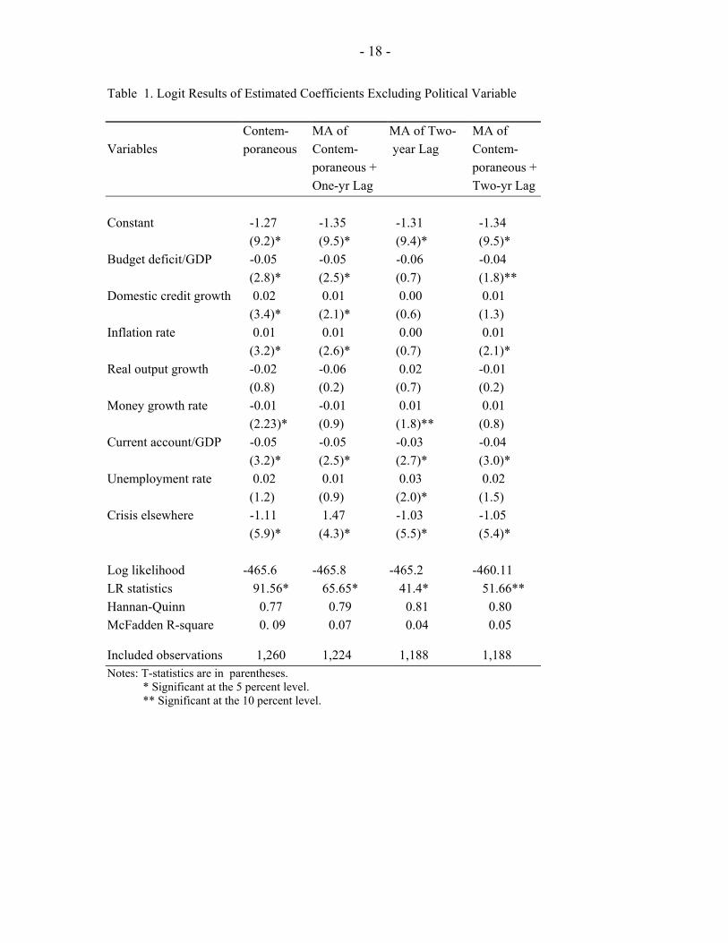
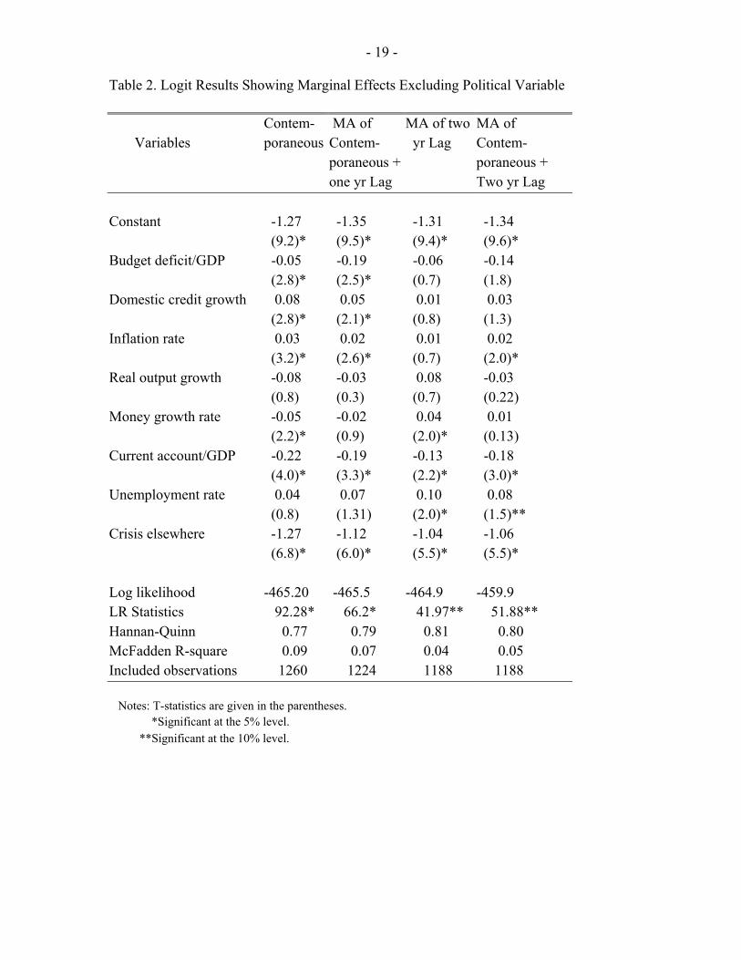
The maximum likelihood binary logit regression results of equation (17) are shown in Tables 1 and 3, while Tables 2 and 4 represent the marginal effects of these independent variables on the conditional probability that a crisis will occur. Table 2 shows negative and statistically significant coefficients at the 5 percent level for the current account balance as a percent of GDP for each period. When the current account variable is included contemporaneously, a 1 percent increase is associated with a 0.22 percent increase in the likelihood of a currency crisis.

With a worsening current account deficit, the authorities are more likely to devalue the currency, increasing pressure on it and thus increasing the likelihood that the currency will be in crisis. Milesi-Ferretti and Razin (1998) determined that less than a third of all current account reversals are preceded by a currency crisis and that, in general, the two occurrences are distinct events. The budget account deficit as a percent of GDP is significant at the 5 percent level when included contemporaneously and lagged for one year. The significance of this coefficient would suggest that when countries pursue lax fiscal policies, evidenced by ever-increasing budget deficits, the probability of currency crises is increased significantly. The growth rate of domestic credit is also positive and statistically significant at the 5 percent level when included contemporaneously and lagged one period, but is insignificant for all other periods. The significance of this variable further strengthens the argument that weak fiscal policies contribute to currency crises.

Interestingly, the growth rate of money is significant when included contemporaneously and lagged over a two-year period. Similarly, the inflation rate is also statistically significant over the same time period. The level of employment, while not significant when included contemporaneously, becomes so when introduced with a two-year lag. Eichengreen, Rose, and Wyplosz (1996), in their study of contagious currency crises in 20 developed countries, determined that higher inflation and unemployment are associated with increases in the odds of an attack, which could result in a currency crisis.

The contagion variable was statistically significant at the 5 percent level. A currency crisis elsewhere in the world is expected to increase the probability of a domestic crisis. This finding broadly supports other studies on the so-called contagion effect. This effect appears to be very strong, suggesting that, even when a country’s economic fundamentals are sound, it may come under attack if its neighbors are so affected. Finally, the reported likelihood ratio statistic tests the joint null hypothesis that all slope coefficients are zero. The results therefore indicate that the coefficients are jointly significant at the 1 percent level.

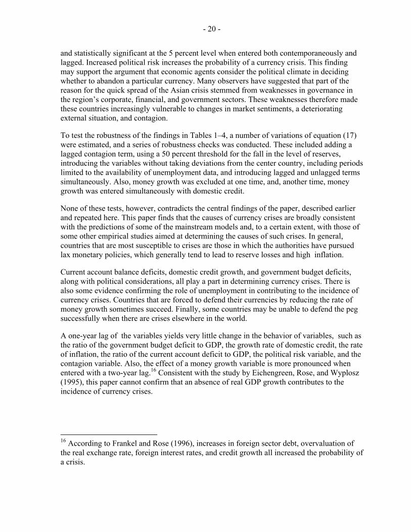
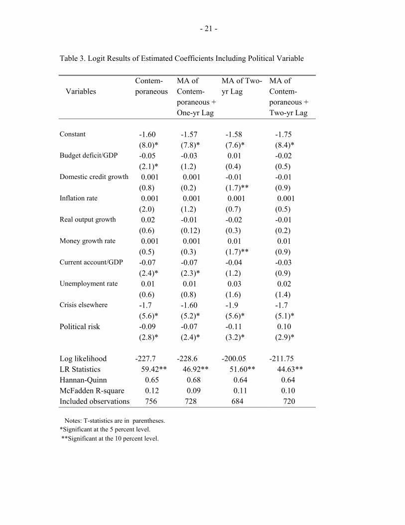
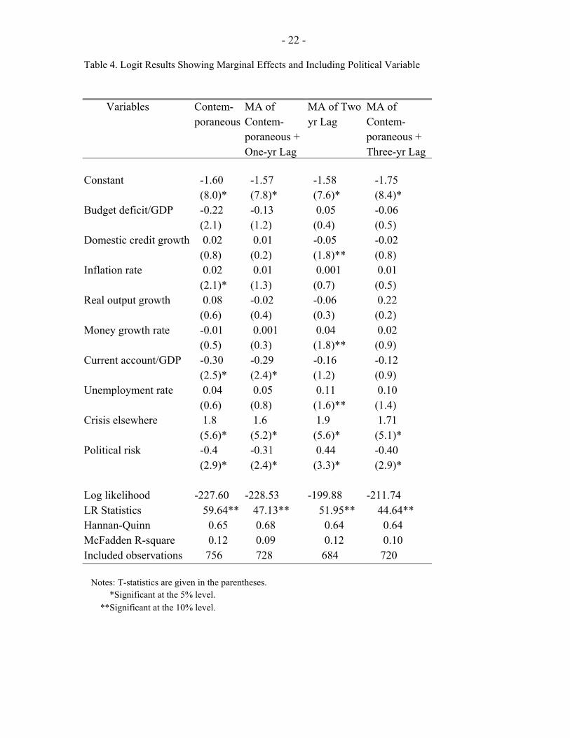
To determine whether political influences also contributed to currency crises over and beyond the macroeconomic effects, the same regressions were run with the inclusion of the political risk variable. Tables 3 and 4 show the results. When the political risk variable is included in the analysis, a number of observations are lost. The variable is, however, positive

- 18 -

Table 1. Logit Results of Estimated Coefficients Excluding Political Variable Contem- MA of MA of Two- MA of Variables poraneous Contem- year Lag Contem- poraneous + poraneous + One-yr Lag Two-yr Lag Constant -1.27 -1.35 -1.31 -1.34 (9.2)* (9.5)* (9.4)* (9.5)* Budget deficit/GDP -0.05 -0.05 -0.06 -0.04 (2.8)* (2.5)* (0.7) (1.8)** Domestic credit growth 0.02 0.01 0.00 0.01 (3.4)* (2.1)* (0.6) (1.3) Inflation rate 0.01 0.01 0.00 0.01 (3.2)* (2.6)* (0.7) (2.1)* Real output growth -0.02 -0.06 0.02 -0.01 (0.8) (0.2) (0.7) (0.2) Money growth rate -0.01 -0.01 0.01 0.01 (2.23)* (0.9) (1.8)** (0.8) Current account/GDP -0.05 -0.05 -0.03 -0.04 (3.2)* (2.5)* (2.7)* (3.0)* Unemployment rate 0.02 0.01 0.03 0.02 (1.2) (0.9) (2.0)* (1.5) Crisis elsewhere -1.11 1.47 -1.03 -1.05 (5.9)* (4.3)* (5.5)* (5.4)* Log likelihood -465.6 -465.8 -465.2 -460.11 LR statistics 91.56* 65.65* 41.4* 51.66** Hannan-Quinn 0.77 0.79 0.81 0.80 McFadden R-square

0. 09 0.07 0.04 0.05

Included observations 1,260 1,224 1,188 1,188 Notes: T-statistics are in parentheses. * Significant at the 5 percent level.

** Significant at the 10 percent level.

- 19 -

Table 2. Logit Results Showing Marginal Effects Excluding Political Variable Contem- MA of MA of two MA of Variables poraneous Contem- yr Lag Contem- poraneous + poraneous + one yr Lag Two yr Lag Constant -1.27 -1.35 -1.31 -1.34 (9.2)* (9.5)* (9.4)* (9.6)* Budget deficit/GDP -0.05 -0.19 -0.06 -0.14 (2.8)* (2.5)* (0.7) (1.8) Domestic credit growth 0.08 0.05 0.01 0.03 (2.8)* (2.1)* (0.8) (1.3) Inflation rate 0.03 0.02 0.01 0.02 (3.2)* (2.6)* (0.7) (2.0)* Real output growth -0.08 -0.03 0.08 -0.03 (0.8) (0.3) (0.7) (0.22) Money growth rate -0.05 -0.02 0.04 0.01 (2.2)* (0.9) (2.0)* (0.13) Current account/GDP -0.22 -0.19 -0.13 -0.18 (4.0)* (3.3)* (2.2)* (3.0)* Unemployment rate 0.04 0.07 0.10 0.08 (0.8) (1.31) (2.0)* (1.5)** Crisis elsewhere -1.27 -1.12 -1.04 -1.06 (6.8)* (6.0)* (5.5)* (5.5)* Log likelihood -465.20 -465.5 -464.9 -459.9 LR Statistics 92.28* 66.2* 41.97** 51.88** Hannan-Quinn 0.77 0.79 0.81 0.80 McFadden R-square 0.09 0.07 0.04 0.05 Included observations 1260 1224 1188 1188 Notes: T-statistics are given in the parentheses. *Significant at the 5% level. **Significant at the 10% level.

- 20 -

and statistically significant at the 5 percent level when entered both contemporaneously and lagged. Increased political risk increases the probability of a currency crisis. This finding may support the argument that economic agents consider the political climate in deciding whether to abandon a particular currency. Many observers have suggested that part of the reason for the quick spread of the Asian crisis stemmed from weaknesses in governance in the region’s corporate, financial, and government sectors. These weaknesses therefore made these countries increasingly vulnerable to changes in market sentiments, a deteriorating external situation, and contagion.

To test the robustness of the findings in Tables 1–4, a number of variations of equation (17) were estimated, and a series of robustness checks was conducted. These included adding a lagged contagion term, using a 50 percent threshold for the fall in the level of reserves, introducing the variables without taking deviations from the center country, including periods limited to the availability of unemployment data, and introducing lagged and unlagged terms simultaneously. Also, money growth was excluded at one time, and, another time, money growth was entered simultaneously with domestic credit.

None of these tests, however, contradicts the central findings of the paper, described earlier and repeated here. This paper finds that the causes of currency crises are broadly consistent with the predictions of some of the mainstream models and, to a certain extent, with those of some other empirical studies aimed at determining the causes of such crises. In general, countries that are most susceptible to crises are those in which the authorities have pursued lax monetary policies, which generally tend to lead to reserve losses and high inflation.

Current account balance deficits, domestic credit growth, and government budget deficits, along with political considerations, all play a part in determining currency crises. There is also some evidence confirming the role of unemployment in contributing to the incidence of currency crises. Countries that are forced to defend their currencies by reducing the rate of money growth sometimes succeed. Finally, some countries may be unable to defend the peg successfully when there are crises elsewhere in the world.

A one-year lag of the variables yields very little change in the behavior of variables, such as the ratio of the government budget deficit to GDP, the growth rate of domestic credit, the rate of inflation, the ratio of the current account deficit to GDP, the political risk variable, and the contagion variable. Also, the effect of a money growth variable is more pronounced when entered with a two-year lag.16 Consistent with the study by Eichengreen, Rose, and Wyplosz (1995), this paper cannot confirm that an absence of real GDP growth contributes to the incidence of currency crises.

16 According to Frankel and Rose (1996), increases in foreign sector debt, overvaluation of the real exchange rate, foreign interest rates, and credit growth all increased the probability of a crisis.

- 21 -

Table 3. Logit Results of Estimated Coefficients Including Political Variable Contem- MA of MA of Two- MA of Variables poraneous Contem- yr Lag Contem- poraneous + poraneous + One-yr Lag Two-yr Lag Constant -1.60 -1.57 -1.58 -1.75 (8.0)* (7.8)* (7.6)* (8.4)* Budget deficit/GDP -0.05 -0.03 0.01 -0.02 (2.1)* (1.2) (0.4) (0.5) Domestic credit growth 0.001 0.001 -0.01 -0.01 (0.8) (0.2) (1.7)** (0.9) Inflation rate 0.001 0.001 0.001 0.001 (2.0) (1.2) (0.7) (0.5) Real output growth 0.02 -0.01 -0.02 -0.01 (0.6) (0.12) (0.3) (0.2) Money growth rate 0.001 0.001 0.01 0.01 (0.5) (0.3) (1.7)** (0.9) Current account/GDP -0.07 -0.07 -0.04 -0.03 (2.4)* (2.3)* (1.2) (0.9) Unemployment rate 0.01 0.01 0.03 0.02 (0.6) (0.8) (1.6) (1.4) Crisis elsewhere -1.7 -1.60 -1.9 -1.7 (5.6)* (5.2)* (5.6)* (5.1)* Political risk -0.09 -0.07 -0.11 0.10 (2.8)* (2.4)* (3.2)* (2.9)* Log likelihood -227.7 -228.6 -200.05 -211.75 LR Statistics 59.42** 46.92** 51.60** 44.63** Hannan-Quinn 0.65 0.68 0.64 0.64 McFadden R-square 0.12 0.09 0.11 0.10 Included observations 756 728 684 720 Notes: T-statistics are in parentheses. *Significant at the 5 percent level. **Significant at the 10 percent level.

- 22 -

Table 4. Logit Results Showing Marginal Effects and Including Political Variable Variables Contem- MA of MA of Two MA of poraneous Contem- yr Lag Contem- poraneous + poraneous + One-yr Lag Three-yr Lag Constant -1.60 -1.57 -1.58 -1.75 (8.0)* (7.8)* (7.6)* (8.4)* Budget deficit/GDP -0.22 -0.13 0.05 -0.06 (2.1) (1.2) (0.4) (0.5) Domestic credit growth 0.02 0.01 -0.05 -0.02 (0.8) (0.2) (1.8)** (0.8) Inflation rate 0.02 0.01 0.001 0.01 (2.1)* (1.3) (0.7) (0.5) Real output growth 0.08 -0.02 -0.06 0.22 (0.6) (0.4) (0.3) (0.2) Money growth rate -0.01 0.001 0.04 0.02 (0.5) (0.3) (1.8)** (0.9) Current account/GDP -0.30 -0.29 -0.16 -0.12 (2.5)* (2.4)* (1.2) (0.9) Unemployment rate 0.04 0.05 0.11 0.10 (0.6) (0.8) (1.6)** (1.4) Crisis elsewhere 1.8 1.6 1.9 1.71 (5.6)* (5.2)* (5.6)* (5.1)* Political risk -0.4 -0.31 0.44 -0.40 (2.9)* (2.4)* (3.3)* (2.9)* Log likelihood -227.60 -228.53 -199.88 -211.74 LR Statistics 59.64** 47.13** 51.95** 44.64** Hannan-Quinn 0.65 0.68 0.64 0.64 McFadden R-square 0.12 0.09 0.12 0.10 Included observations 756 728 684 720 Notes: T-statistics are given in the parentheses. *Significant at the 5% level. **Significant at the 10% level.

- 23 -

E. Results Based on a Comparison Between Developed and Emerging Market Economies

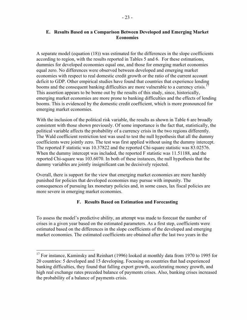
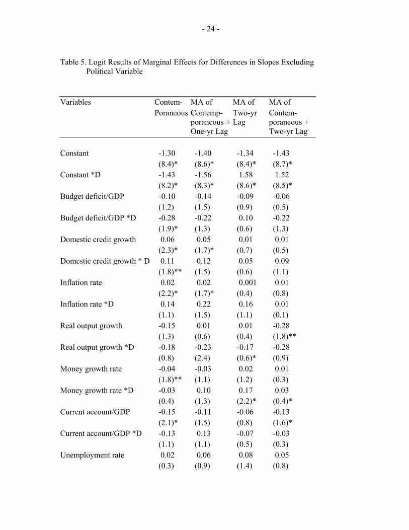
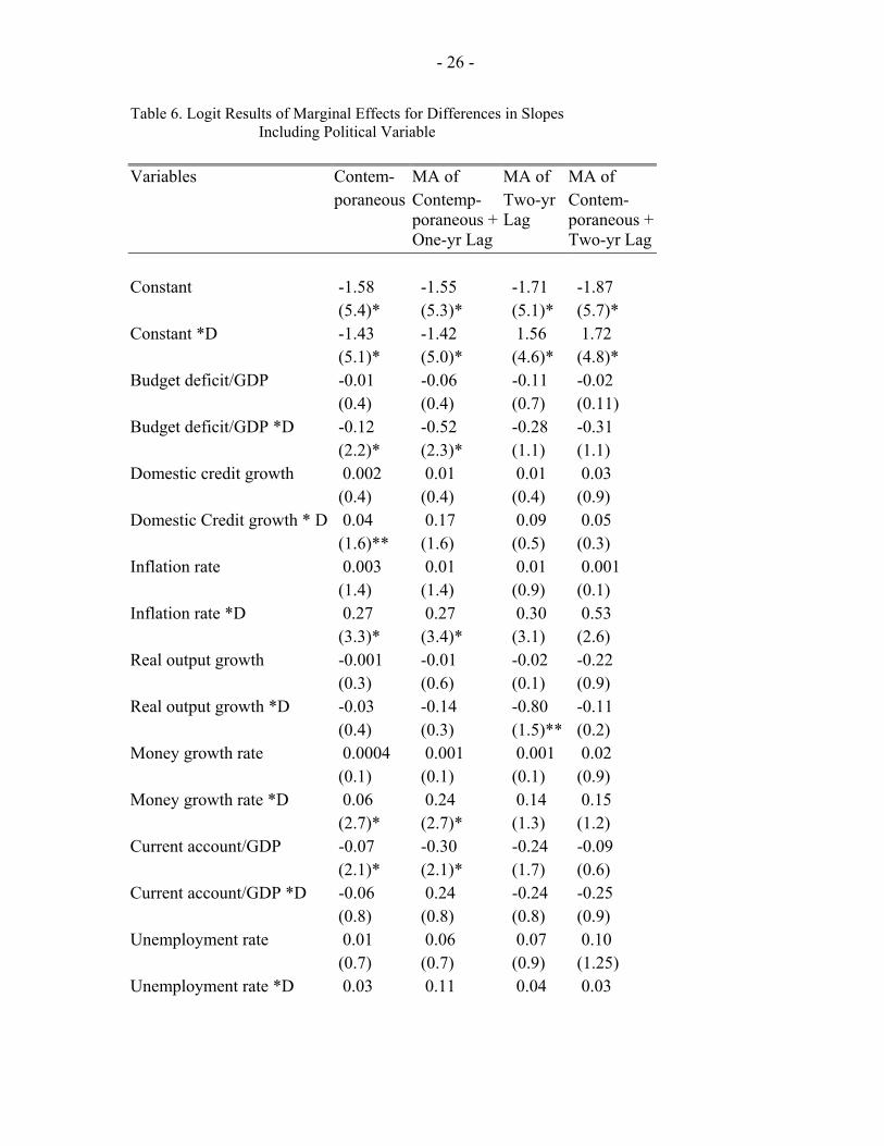
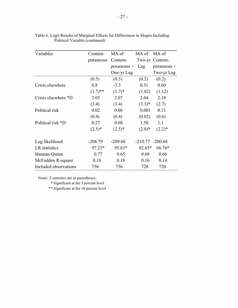
A separate model (equation (18)) was estimated for the differences in the slope coefficients according to region, with the results reported in Tables 5 and 6. For these estimations, dummies for developed economies equal one, and those for emerging market economies equal zero. No differences were observed between developed and emerging market economies with respect to real domestic credit growth or the ratio of the current account deficit to GDP. Other empirical studies have found that countries that experience lending booms and the consequent banking difficulties are more vulnerable to a currency crisis.17 This assertion appears to be borne out by the results of this study, since, historically, emerging market economies are more prone to banking difficulties and the effects of lending booms. This is evidenced by the domestic credit coefficient, which is more pronounced for emerging market economies.

With the inclusion of the political risk variable, the results as shown in Table 6 are broadly consistent with those shown previously. Of some importance is the fact that, statistically, the political variable affects the probability of a currency crisis in the two regions differently. The Wald coefficient restriction test was used to test the null hypothesis that all the dummy coefficients were jointly zero. The test was first applied without using the dummy intercept. The reported F statistic was 10.37822 and the reported Chi-square statistic was 83.02576. When the dummy intercept was included, the reported F statistic was 11.51188, and the reported Chi-square was 103.6070. In both of these instances, the null hypothesis that the dummy variables are jointly insignificant can be decisively rejected.

Overall, there is support for the view that emerging market economies are more harshly punished for policies that developed economies may pursue with impunity. The consequences of pursuing lax monetary policies and, in some cases, lax fiscal policies are more severe in emerging market economies.

F. Results Based on Estimation and Forecasting

To assess the model’s predictive ability, an attempt was made to forecast the number of crises in a given year based on the estimated parameters. As a first step, coefficients were estimated based on the differences in the slope coefficients of the developed and emerging market economies. The estimated coefficients are obtained after the last two years in the

17 For instance, Kaminsky and Reinhart (1996) looked at monthly data from 1970 to 1995 for 20 countries: 5 developed and 15 developing. Focusing on countries that had experienced banking difficulties, they found that falling export growth, accelerating money growth, and high real exchange rates preceded balance of payments crises. Also, banking crises increased the probability of a balance of payments crisis.

- 24 -

Table 5. Logit Results of Marginal Effects for Differences in Slopes Excluding

Political Variable Variables Contem- MA of MA of MA of Poraneous Contemp-

poraneous +Two-yr Lag

Contem-poraneous +

One-yr Lag Two-yr Lag Constant -1.30 -1.40 -1.34 -1.43 (8.4)* (8.6)* (8.4)* (8.7)* Constant *D -1.43 -1.56 1.58 1.52 (8.2)* (8.3)* (8.6)* (8.5)* Budget deficit/GDP -0.10 -0.14 -0.09 -0.06 (1.2) (1.5) (0.9) (0.5) Budget deficit/GDP *D -0.28 -0.22 0.10 -0.22 (1.9)* (1.3) (0.6) (1.3) Domestic credit growth 0.06 0.05 0.01 0.01 (2.3)* (1.7)* (0.7) (0.5) Domestic credit growth * D 0.11 0.12 0.05 0.09 (1.8)** (1.5) (0.6) (1.1) Inflation rate 0.02 0.02 0.001 0.01 (2.2)* (1.7)* (0.4) (0.8) Inflation rate *D 0.14 0.22 0.16 0.01 (1.1) (1.5) (1.1) (0.1) Real output growth -0.15 0.01 0.01 -0.28 (1.3) (0.6) (0.4) (1.8)** Real output growth *D -0.18 -0.23 -0.17 -0.28 (0.8) (2.4) (0.6)* (0.9) Money growth rate -0.04 -0.03 0.02 0.01 (1.8)** (1.1) (1.2) (0.3) Money growth rate *D -0.03 0.10 0.17 0.03 (0.4) (1.3) (2.2)* (0.4)* Current account/GDP -0.15 -0.11 -0.06 -0.13 (2.1)* (1.5) (0.8) (1.6)* Current account/GDP *D -0.13 0.13 -0.07 -0.03 (1.1) (1.1) (0.5) (0.3) Unemployment rate 0.02 0.06 0.08 0.05 (0.3) (0.9) (1.4) (0.8)

- 25 -

Table 5. Logit Results of Marginal Effects for Differences in Slopes Excluding Political Variable (continued)

Variables Contem- MA of MA of MA of poraneous Contem- Two-yr Contem- poraneous + Lag poraneous + One yr lag Two-yr lag Crisis elsewhere -0.7 -0.6 0.5 0.33 (2.9)* (2.4)* (2.1)* (1.3) Crisis elsewhere*D -1.34 -1.25 1.26 1.4 (4.2)* (3.7) (3.8)* (4.1) Log likelihood -453.36 -452.21 -452.66 -449.53 LR Statistics 115.96* 92.87* 66.55* 72.82* Hannan-Quinn 0.77 0.79 0.82 0.81 McFadden R-square 0.11 0.09 0.07 0.07 Included observations 1260 1224 1188 1188 Notes: t-statistics are given in the parentheses. * Significant at the 5% level. ** Significant at the 10% level.

- 26 -

Table 6. Logit Results of Marginal Effects for Differences in Slopes Including Political Variable

Variables Contem- MA of MA of MA of poraneous Contemp-

poraneous +Two-yr Lag

Contem-poraneous +

One-yr Lag Two-yr Lag Constant -1.58 -1.55 -1.71 -1.87 (5.4)* (5.3)* (5.1)* (5.7)* Constant *D -1.43 -1.42 1.56 1.72 (5.1)* (5.0)* (4.6)* (4.8)* Budget deficit/GDP -0.01 -0.06 -0.11 -0.02 (0.4) (0.4) (0.7) (0.11) Budget deficit/GDP *D -0.12 -0.52 -0.28 -0.31 (2.2)* (2.3)* (1.1) (1.1) Domestic credit growth 0.002 0.01 0.01 0.03 (0.4) (0.4) (0.4) (0.9) Domestic Credit growth * D 0.04 0.17 0.09 0.05 (1.6)** (1.6) (0.5) (0.3) Inflation rate 0.003 0.01 0.01 0.001 (1.4) (1.4) (0.9) (0.1) Inflation rate *D 0.27 0.27 0.30 0.53 (3.3)* (3.4)* (3.1) (2.6) Real output growth -0.001 -0.01 -0.02 -0.22 (0.3) (0.6) (0.1) (0.9) Real output growth *D -0.03 -0.14 -0.80 -0.11 (0.4) (0.3) (1.5)** (0.2) Money growth rate 0.0004 0.001 0.001 0.02 (0.1) (0.1) (0.1) (0.9) Money growth rate *D 0.06 0.24 0.14 0.15 (2.7)* (2.7)* (1.3) (1.2) Current account/GDP -0.07 -0.30 -0.24 -0.09 (2.1)* (2.1)* (1.7) (0.6) Current account/GDP *D -0.06 0.24 -0.24 -0.25 (0.8) (0.8) (0.8) (0.9) Unemployment rate 0.01 0.06 0.07 0.10 (0.7) (0.7) (0.9) (1.25) Unemployment rate *D 0.03 0.11 0.04 0.03

- 27 -

Table 6. Logit Results of Marginal Effects for Differences in Slopes Including Political Variable (continued)

Variables Contem- MA of MA of MA of poraneous Contem- Two-yr Contem- poraneous + Lag poraneous + One-yr Lag Two-yr Lag (0.5) (0.5) (0.2) (0.2) Crisis elsewhere 0.8 -3.3 0.51 0.60 (1.7)** (1.7)* (1.02) (1.12) Crisis elsewhere *D 3.05 3.07 2.64 2.18 (3.4) (3.4) (3.3)* (2.7) Political risk 0.02 0.06 0.001 0.11 (0.4) (0.4) (0.02) (0.6) Political risk *D 0.27 0.08 1.50 1.1 (2.5)* (2.5)* (2.8)* (2.2)* Log likelihood -208.79 -209.60 -210.77 -200.68 LR statistics 97.23* 95.63* 82.65* 66.76* Hannan-Quinn 0.77 0.65 0.68 0.66 McFadden R-square 0.18 0.18 0.16 0.14 Included observations 756 756 728 720 Notes: T-statistics are in parentheses; * Significant at the 5 percent level ** Significant at the 10 percent level

- 28 -

sample are excluded. For the most part, the results do not differ to any significant extent with those obtained when all the years are included.

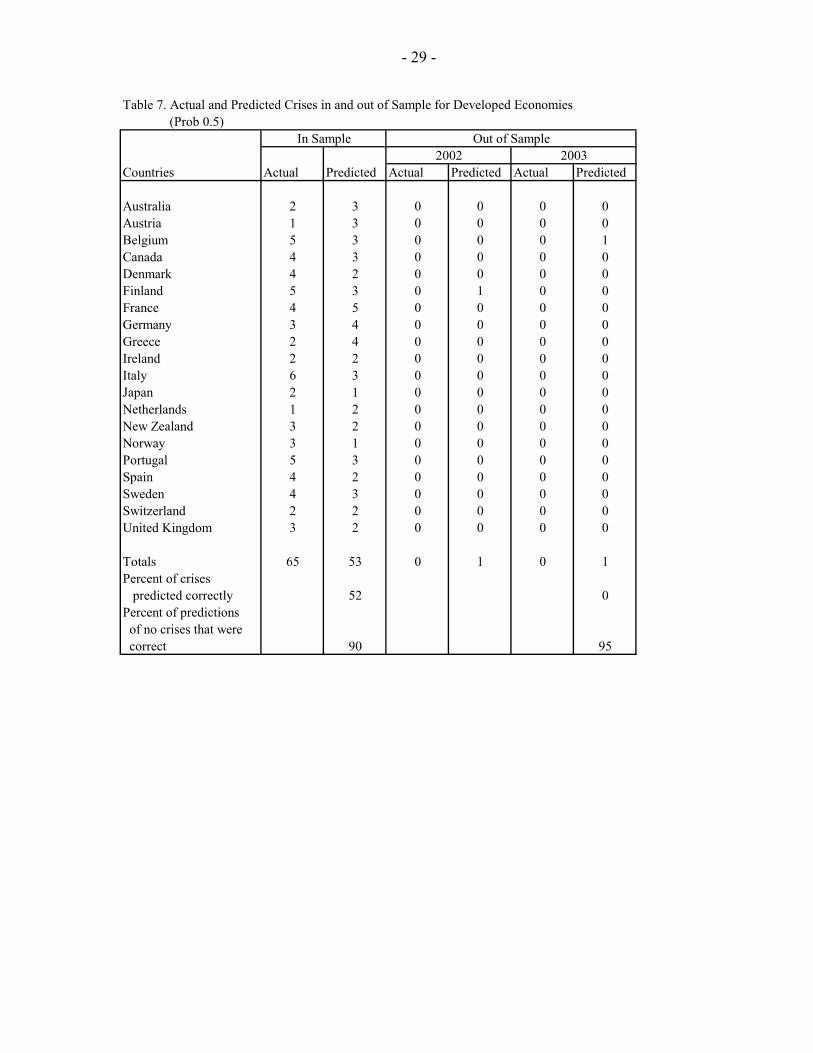
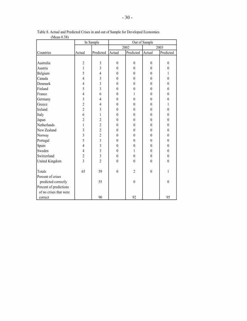
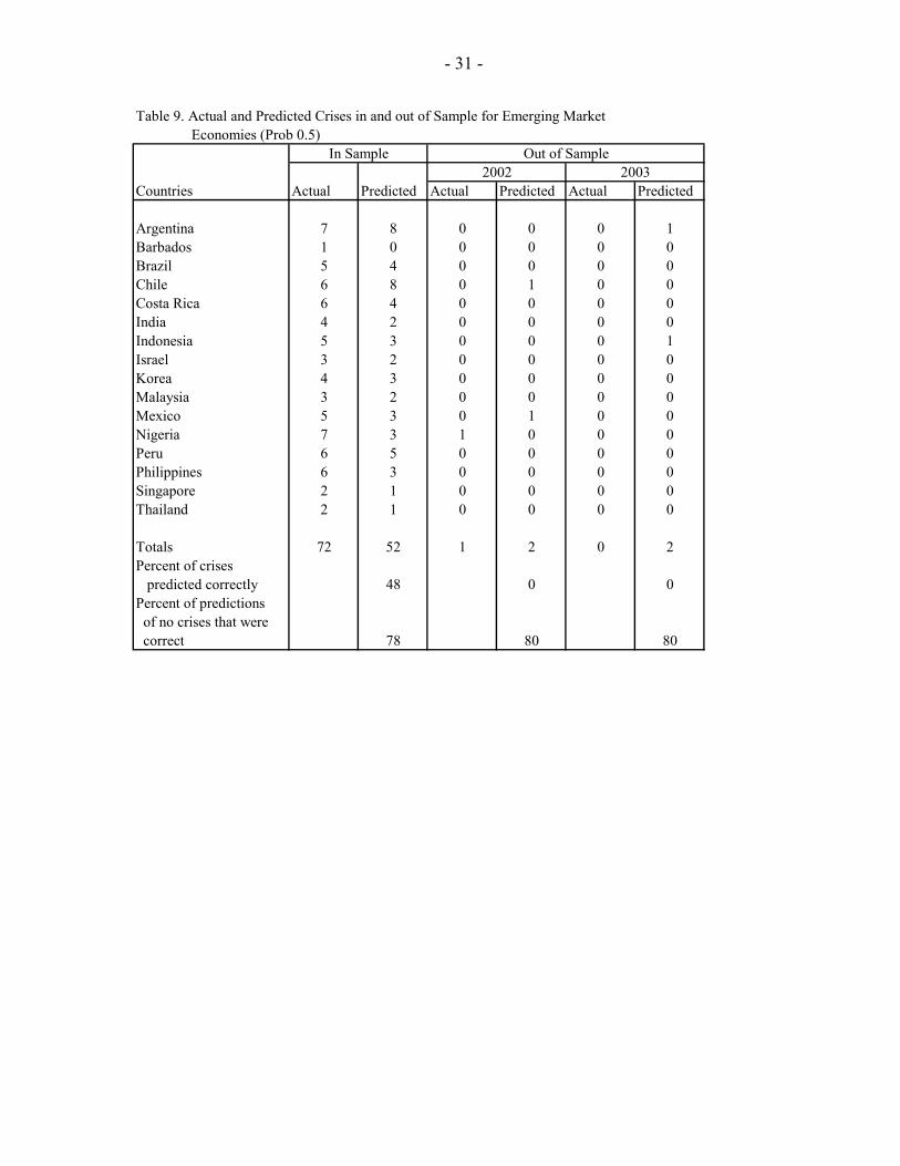
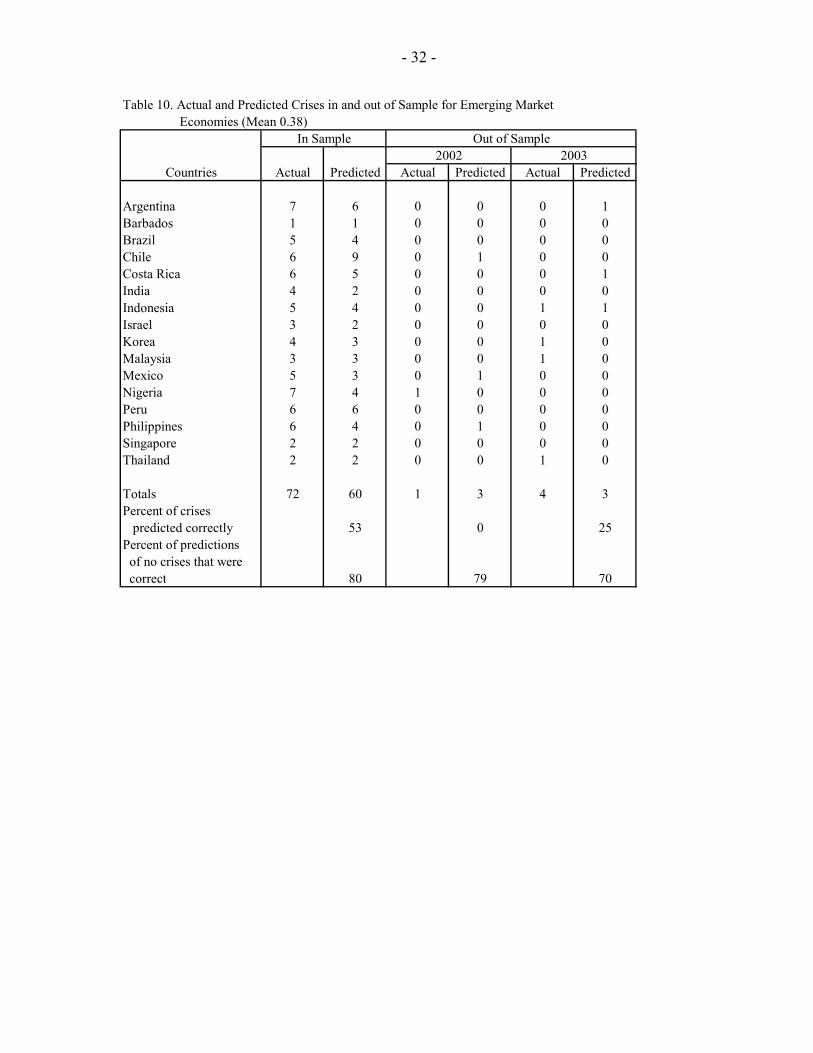
Fitted probabilities are then computed on the basis of the estimated coefficients of the adjusted sample. These probabilities are then used to predict crises for the different countries throughout the period. A probability value of 0.5 or greater is used in determining the occurrence of a crisis. As an alternative, the mean of the data is the determining value used. Tables 7-10 show the number of crises predicted using these alternative measures. To facilitate comparison, the actual number of crises based on the sample data and the definition of a crisis outlined earlier are also shown.

Overall, the model met with only limited success in forecasting crises in both the developed and the emerging market economies for the out-of-sample period. These were generally periods in which a large number of countries in the group experienced severe problems associated with their currencies. Over the entire sample period, a greater number of crises were forecast for the emerging market economies than for the developed economies. Where the probability values were adopted in determining the forecasts, a smaller number of crises were generally forecast, compared with the mean value.

For the developed economies, 52 percent of the crises were correctly predicted in sample when the probability value was used, increasing to 55 percent with the use of the mean value of 0.38. In the emerging market economies, 48 percent of the crises were correctly predicted, with a probability value of 0.5 and 53 percent with a mean value of 0.38.

V. CONCLUSION

This paper examined the effect of macroeconomic variables, a contagion variable, and political considerations in determining currency crises in 37 developed and emerging market economies during 1968–2003. To evaluate the impact of these variables, the probability of a currency crisis as a function of these fundamentals was computed by using the implications of the various theoretical models of currency crises.

The literature contains a number of theoretical models that attempt to explain the dynamics behind currency crises. Fundamental to these models is why authorities either choose or are forced by unavoidable events to abandon the exchange rate regime, with the reasons ranging from an emphasis on bad fundamentals to the role of speculative agents in precipitating a currency crisis. Other models focus attention on the role that political influences play in making it difficult to defend the exchange rate regime successfully, and some stress the role of contagion in affecting otherwise solid currency arrangements.

This paper tested empirically the implications of those models. By focusing on a broad range of countries with varying economic and political situations, I have attempted to determine the extent to which these variables increase the probability that a currency crisis will occur. While no attempt is made empirically to differentiate explicitly between first-and-second generation models, the paper finds compelling evidence that both of these theoretical underpinnings are borne out by the available evidence.

- 29 -

Table 7. Actual and Predicted Crises in and out of Sample for Developed Economies (Prob 0.5)

Countries Actual Predicted Actual Predicted Actual Predicted

Australia 2 3 0 0 0 0Austria 1 3 0 0 0 0Belgium 5 3 0 0 0 1Canada 4 3 0 0 0 0Denmark 4 2 0 0 0 0Finland 5 3 0 1 0 0France 4 5 0 0 0 0Germany 3 4 0 0 0 0Greece 2 4 0 0 0 0Ireland 2 2 0 0 0 0Italy 6 3 0 0 0 0Japan 2 1 0 0 0 0Netherlands 1 2 0 0 0 0New Zealand 3 2 0 0 0 0Norway 3 1 0 0 0 0Portugal 5 3 0 0 0 0Spain 4 2 0 0 0 0Sweden 4 3 0 0 0 0Switzerland 2 2 0 0 0 0United Kingdom 3 2 0 0 0 0

Totals 65 53 0 1 0 1Percent of crises predicted correctly 52 0Percent of predictions of no crises that were correct 90 95

2002 2003In Sample Out of Sample

- 30 -

Table 8. Actual and Predicted Crises in and out of Sample for Developed Economies

Countries Actual Predicted Actual Predicted Actual Predicted

Australia 2 3 0 0 0 0Austria 1 3 0 0 0 0Belgium 5 4 0 0 0 1Canada 4 3 0 0 0 0Denmark 4 3 0 0 0 0Finland 5 3 0 0 0 0France 4 6 0 1 0 0Germany 3 4 0 0 0 0Greece 2 4 0 0 0 1Ireland 2 3 0 0 0 0Italy 6 1 0 0 0 0Japan 2 2 0 0 0 0Netherlands 1 2 0 0 0 0New Zealand 3 2 0 0 0 0Norway 3 2 0 0 0 0Portugal 5 3 0 0 0 0Spain 4 3 0 0 0 0Sweden 4 3 0 1 0 0Switzerland 2 3 0 0 0 0United Kingdom 3 2 0 0 0 0

Totals 65 59 0 2 0 1Percent of crises predicted correctly 55 0 0Percent of predictions of no crises that were correct 90 92 95

2002 2003

(Mean 0.38)In Sample Out of Sample

- 31 -

Table 9. Actual and Predicted Crises in and out of Sample for Emerging Market

Countries Actual Predicted Actual Predicted Actual Predicted

Argentina 7 8 0 0 0 1Barbados 1 0 0 0 0 0Brazil 5 4 0 0 0 0Chile 6 8 0 1 0 0Costa Rica 6 4 0 0 0 0India 4 2 0 0 0 0Indonesia 5 3 0 0 0 1Israel 3 2 0 0 0 0Korea 4 3 0 0 0 0Malaysia 3 2 0 0 0 0Mexico 5 3 0 1 0 0Nigeria 7 3 1 0 0 0Peru 6 5 0 0 0 0Philippines 6 3 0 0 0 0Singapore 2 1 0 0 0 0Thailand 2 1 0 0 0 0

Totals 72 52 1 2 0 2Percent of crises predicted correctly 48 0 0Percent of predictions of no crises that were correct 78 80 80

2002 2003

Economies (Prob 0.5)In Sample Out of Sample

- 32 -

Table 10. Actual and Predicted Crises in and out of Sample for Emerging Market

Countries Actual Predicted Actual Predicted Actual Predicted

Argentina 7 6 0 0 0 1Barbados 1 1 0 0 0 0Brazil 5 4 0 0 0 0Chile 6 9 0 1 0 0Costa Rica 6 5 0 0 0 1India 4 2 0 0 0 0Indonesia 5 4 0 0 1 1Israel 3 2 0 0 0 0Korea 4 3 0 0 1 0Malaysia 3 3 0 0 1 0Mexico 5 3 0 1 0 0Nigeria 7 4 1 0 0 0Peru 6 6 0 0 0 0Philippines 6 4 0 1 0 0Singapore 2 2 0 0 0 0Thailand 2 2 0 0 1 0

Totals 72 60 1 3 4 3Percent of crises predicted correctly 53 0 25Percent of predictions of no crises that were correct 80 79 70

2002 2003

Economies (Mean 0.38)In Sample Out of Sample

- 33 -

The empirical findings support the view that, in general, a deterioration in economic fundamentals and pursuit of lax monetary policy can contribute to currency crises. Unfavorable political factors and currency crises elsewhere in the world may make a crisis more likely. The Asian crisis highlighted the need for instruments and mechanisms that will discourage private sector investors from withdrawing from a country facing a potential loss of market access. More important is the need to inhibit the buildup of financial vulnerabilities that make a crisis likely and more difficult to resolve.

An important distinguishing feature of this paper is that it compares the incidence of currency crises in both developed and developing countries. The evidence suggests that emerging market economies suffer more than developed economies if they pursue lax monetary and fiscal policies. But both groups of economies appear to be equally affected by political considerations.

The effect of some of the variables that contribute to currency crises is more pronounced in emerging market economies. In particular, during 1968–2001, the growth rate of domestic credit, the rate of inflation, and the growth rate of money all played a more significant role in emerging market economies than in developed economies in determining currency crises. Also during that period, low output growth, the current account deficit, and the budget deficit all contributed to the recorded crises.

Although no effort was made to determine how currency crises were transmitted from one country to another, the paper establishes the existence of contagion in foreign exchange markets. The experiences of several emerging market economies suggest that the sustainability of exchange rate policy depends on adequate policy responses to economic shocks, and the fragility of the economic and financial system as well as the political system.

The attempt to forecast crises by directly estimating the probability of a currency crisis and identifying the variables that were significant in predicting it met with only limited success because, admittedly, the timing of crises may depend on variables that are hard to capture, such as institutional development, structural features, and expectations of domestic and foreign economic agents. Also, the whole question of policy responses and policymaking—themselves difficult to capture—would be critical in determining whether a crisis occurs or is contained early on. Not surprisingly, these variables were not taken into account in the analysis, thus limiting the success of the model in predicting the timing of crises.

Further, it was important to assume that the relevant variables were similar across time and countries. This assumption is clearly not correct, given the diversity of countries. It is also quite possible that the increasing globalization of financial markets and the speed with which countries succumb to changes coming from outside could cause certain variables to change over time even within the same country. Successfully predicting crises therefore requires the ability to model variables, which are themselves difficult, if not impossible, to measure. But giving policymakers early warning of such crises is clearly desirable, and further research into the timing of such crises is needed.

The analysis did not explicitly capture what happens when a country chooses to devalue. Clearly, large devaluations can be perceived as crises. This paper, rather than rely on

- 34 -

instances when a country devalues, assumed that large losses in reserves could very well cover these episodes. This may not always be the case. The paper found support for the view that a strong domestic financial system, coupled with consistent fiscal and monetary policies, is key to sustaining any exchange rate regime. The implementation of consistent macroeconomic policies may involve politically difficult decisions, and, thus, the maintenance of any exchange rate regime is greatly aided by broad political support for the chosen regime and for the policies needed to underpin the sustainability of the exchange rate regime.

- 35 -

REFERENCES Agenor, Pierre-Richard, Jagdeep S. Bhandari, and Robert P. Flood, 1992, “Speculative Attacks and Models of Balance-of-Payments Crises,” IMF Staff Papers, Vol. 39 (June), pp. 357-94. Agenor, Pierre-Richard, and Robert P. Flood, 1994,. “Macroeconomics Policy, Speculative Attacks, and Balance of Payments Crises,” in the Handbook of International Macroeconomics, ed. by Frederick Van Der Ploeg (Cambridge, Massachusetts, and Oxford, England: Blackwell), pp. 612-32. Andersen, Torben, M.. 1994, “Shocks and the Viability of a Fixed Exchange Rate Commitment.” CEPR Discussion Paper 969 (London: Centre for Economic Policy Research). Berg, Andrew, and Catherine Pattillo, 1998, “Are Currency Crises Predictable? A Test.” IMF Working Paper 98/154 (Washington: International Monetary Fund). Berg, Andrew, Eduardo Borensztein, and Catherine Pattillo, 2004, “Assessing Early Warning Systems: How Have They Worked in Practice?” IMF Working Paper 04/52 (Washington: International Monetary Fund). Blackburn Keith, and Martin Sola, 1993,. “Speculative Currency Attacks and Balance of Payments Crises,” Journal of Economic Surveys, Vol. 7, (June) , pp.119–44. Bordo, Michael, and Anna J. Schwartz, 1996, “Why Clashes Between Internal and External Stability Goals End in Currency Crises, 1797-1994,” Open Economies Review, Vol. 7 (Supplement), pp. 437–68. Brown, William Adams, Jr., 1940,. “The International Gold Standard Reinterpreted, 1914- 1934” (New York: National Bureau of Economic Research). Buiter, Willem, Giancarlo Corsetti, and Paolo Pesenti, 1995,. “A Center Periphery Model of Monetary Coordination and Exchange Rate Crisis,” NBER Working Paper 5140 (Cambridge, Massachusetts: National Bureau of Economic Research). Calvo, Sara, and Carmen M. Reinhart, 1996, “Capital Flows to Latin America: Is there Evidence of Contagion Effects?” in Capital Flows to Developing Economies, ed. By Morris Goldstein (Washington: Institute for International Economics). Dornbusch, Rudiger, Ilan Goldfajn, and Rodrigo O. Valdes, 1995, “Currency Crises and Collapses,” Brookings Papers on Economic Activity: 2, 219–93. Duttagupta, Rupa, Gilda Fernandez, and Cem Karacadag, 2004,. “From Fixed to Float: Operational Aspects of Moving Towards Exchange Rate Flexibility,” IMF Working Paper 04/126 (Washington: International Monetary Fund).

- 36 -

Eichengreen, Barry, Andrew K. Rose, and Charles Wyplosz, 1995,. “Exchange Market Mayhem: The Antecedents and Aftermath of Speculative Attacks, “ Economic Policy Vol. 21 (October), pp. 249–312. ______, 1996, “Contagious Currency Crises,” NBER Working Paper 5681 (Cambridge, Massachusetts: National Bureau of Economic Research).. Eichengreen, Barry, and Chang-Tai Hsieh, 1996, “Sterling in Decline Again: The 1931 and 1992 Crises Compared,” in European Economic Integration as a Challenge to Industry and Government, ed by Richard Tilly and Paul J.J. Welfens (New York: Springer-Verlag). Flood, Robert P., and Peter M. Garber, 1984, “Collapsing Exchange-Rate Regimes: Some Linear Examples,” Journal of International Economics Vol. 17 (August),pp. 1–13. Flood, Robert P., and Nancy Marion,1996,. “ Speculative Attacks: Fundamentals and Self- fulfilling Prophecies,” NBER Working Paper 5789 (Caambridge, Massachusetts: National Bureau of Economic Research). Frankel, Jeffrey, and Steven Philips, 1992, “The European Monetary System: Credible at Last?” Oxford Economic Papers, Vol. 44 (October), pp. 259–84. Frankel, Jeffrey, and Andrew K. Rose, 1996, “Currency Crashes in Emerging Markets: Empirical Indicators,” NBER Working Paper 5437 (Cambridge, Massachusetts: National Bureau of Economic Research). . Funke, Norbert, 1996, “Vulnerability of Fixed Exchange Rate Regimes: The Role of Economic Fundamentals,” OECD Economic Studies No. 26, 158–176.?? Garber, Peter, M.,1990,. “Famous First Bubbles,” Journal of Economic Perspectives, Vol. 4 (month), pp. 35–54. Gerlach, Stefan, and Frank Smets, 1995,. “Contagious Speculative Attacks.” European Journal of Political Economy, Vol. 11 (March), pp. 45–63. Girton, Lance, and Don Roper, 1977, “ A Monetary Model of Exchange Market Pressure Applied to the Postwar Canadian Experience,” American Economic Review Vol. 67 (month), pp. 537–48. Goldberg, Linda S., 1994, “Predicting Exchange Rate Crises─Mexico Revisited,” Journal of International Economics Vol. 36 (May), pp. 413-30. Jeanne, Olivier, 1997, “Are Currency Crises Self-Fulfilling? A Test.” Journal of International Economics Vol. 43 (November), pp. 263–86.

- 37 -

Kaminsky, Graciela, and Carmen M. Reinhart, 1996, “The Twin Crises,” FRBDiscussion Paper No. 544 (Washington: Board of Governors of the Federal Reserve System, International Finance Division). Kaminsky, Graciela, Saul Lizondo, and Carmen M. Reinhart, 1998,. “Leading Indicators of Currency Crises, ” IMF Staff Papers Vol. 45 (March), pp. 1–48. Krugman, Paul, 1979, “A Model of Balance-of -Payments Crises,” Journal of Money, Credit and Banking, Vol. 11 (month), p. 311-25. Masson, Paul, R., 1995, “Gaining and Losing ERM Credibility: The Case of the United Kingdom,” Economic Journal, Vol. 105 (May), pp. 571–82. Milesi-Ferretti, Gian Maria, and Assaf Razin, 1998, “Current Account Reversals and Currency Crises: Empirical Regularities,” IMF Working Paper 98/89 (Washington: International monetary Fund). O’Brien, Patrick, 1958-60?. “Government Revenue, 1793- 815: A Study in Fiscal and Financial Policy in the Wars Against France” (unpublished; Oxford, England?: Oxford University). Obstfeld, Maurice, 1994,. “The Logic of Currency Crises,” Cahiers Economiques et Monétaires No. 44 (Paris: Banque de France). ________, 1996,. “Models of Currency Crises with Self-fulfilling Features,” European Economic Review, Vol. 40 (April), pp. 1037–1047. Otker, Inci, and Ceyla Pazarbagioglu,1996, “Speculative Attacks and Currency Crisis: The Mexican Experience,” Open Economics Review, Vol. 7 (Supplement 1), pp. 535– 52. Ozkan, Gulcin F., and Alan Sutherland, 1995,. “Policy Measures to Avoid a Currency Crisis,” Journal of the Royal Economic Society, Vol. 105 (March), pp. 510–19. Sachs Jefferey D., Aaron Tornell, and Andres Velasco, 1996, “ Financial Crisis in Developing Economies: The Lessons From 1995,” Brookings Papers on Economic Activity: 1, pp.147-215. Salant, Stephen, and Dale Henderson, 1978,. “Market Anticipation of Government Policy and the Price of Gold,” Journal of Political Economy, Vol. 86 (August), pp. 627-48. Tudela, Merxe, 2004, “Explaining Currency Crises: A Duration Model Approach” Journal of International Money and Finance, Vol. 23 (September), pp. 799–816. Velasco, Andres, 1987, “Financial Crises and Balance of Payments Crises: A Simple Model of the Southern Cone Experience,” Journal of Development Economics, Vol. 27 (October), pp. 263–83.