EELLEEGG666677:: FFiinnaall pprroojjeecctt rreeppoorrtt 

 

CCUUDDAA bbaasseedd iimmpplleemmeennttaattiioonn ooff

DDCCTT//IIDDCCTT oonn GGPPUU 

Team member: Peng Ye

Xiaoyan Shi

Instructor: Xiaoming Li 

 

U N I V E R S I T Y   O F   D E L A W A R E  

1  

Contents 

A. Introduction to DCT/IDCT B. Direct matrix multiplication algorithm implementation 

1. Implementation on CPU 2. Implementation on GPU 

C. FFT based algorithm implementation 1. Algorithm description 2. Implementation on CPU 3. Implementation on GPU 

D. Conclusion 

   

 

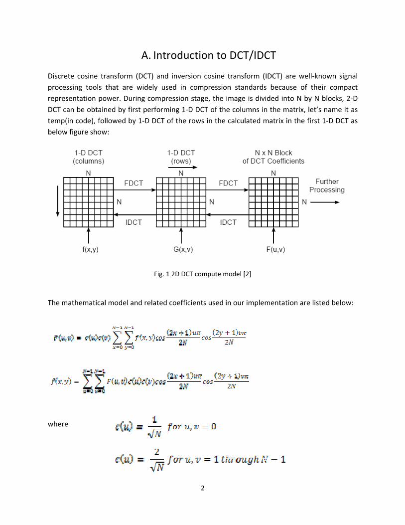
Discrete processinrepresenDCT can temp(in below fig

 

  The math 

 

 

 

 

 

where 

 

 

cosine  tranng  tools  thantation powebe obtainedcode), followgure show: 

hematical m

A. sform  (DCTat  are  wideer. During cod by first pewed by 1‐D 

model and rel

Introdu

) and  inversely  used  in ompression rforming 1‐DDCT of the r

Fig. 1 2D DC

lated coeffic

2 

ction to 

sion  cosine compressiostage, the  iD DCT of therows in the 

T compute m

cients used i

 

DCT/IDC

transform  (n  standardsmage  is dive columns incalculated m

model [2] 

n our implem

CT 

IDCT) are ws  because  oided  into N n the matrixmatrix in the

mentation a

well‐known  sof  their  comby N blocksx, let’s namee first 1‐D DC

re listed bel

signal mpact s, 2‐D e it as CT as 

 

          

ow: 

 

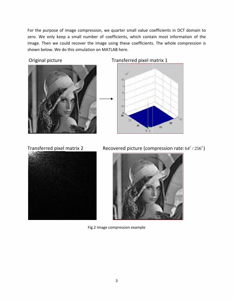
For  the pzero. Weimage. Tshown be

 Origina

 Transfe

 

 

 

purpose of  ie  only  keepThen we  couelow. We do

al picture   

rred pixel 

image compp  a  small  nuuld  recover o this simula

                  

matrix 2    

pression, weumber  of  cothe  image ution on MAT

                 

            

            Rec

            

Fig.2 Image c

3 

e quarter smoefficients, wusing  these TLAB here.

  Transferr

        

covered pi

   

compression 

mall value cowhich  contacoefficients

red pixel m

cture (com

example 

oefficients  inain most  infs. The whole

matrix 1      

mpression 

n DCT domaformation  oe  compressi

                  

 

rate: 264 / 2

 

ain  to f  the ion  is 

     

2256 )                        

4  

B. Direct matrix multiplication algorithm implementation  

1. Implementation on CPU 

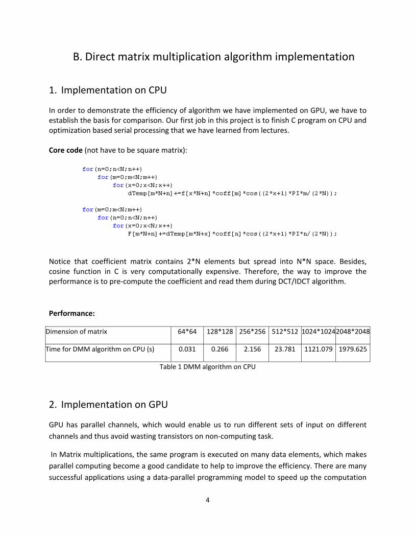
In order to demonstrate the efficiency of algorithm we have implemented on GPU, we have to establish the basis for comparison. Our first job in this project is to finish C program on CPU and optimization based serial processing that we have learned from lectures.  Core code (not have to be square matrix): 

 

 Notice  that  coefficient matrix  contains  2*N  elements  but  spread  into  N*N  space.  Besides, cosine  function  in  C  is  very  computationally  expensive.  Therefore,  the way  to  improve  the performance is to pre‐compute the coefficient and read them during DCT/IDCT algorithm. 

 

Performance: 

Dimension of matrix  64*64  128*128 256*256 512*512  1024*10242048*2048

Time for DMM algorithm on CPU (s)  0.031  0.266  2.156  23.781  1121.079  1979.625

Table 1 DMM algorithm on CPU 

 

2. Implementation on GPU 

GPU has parallel  channels, which would enable us  to  run different  sets of  input on different channels and thus avoid wasting transistors on non‐computing task. 

 In Matrix multiplications, the same program is executed on many data elements, which makes parallel computing become a good candidate to help to improve the efficiency. There are many successful applications using a data‐parallel programming model to speed up the computation 

5  

of  large data  sets  such as matrix. And as a  streaming processor,  the GPU has  some  features which are especially good to address problems for data‐parallel computations. 

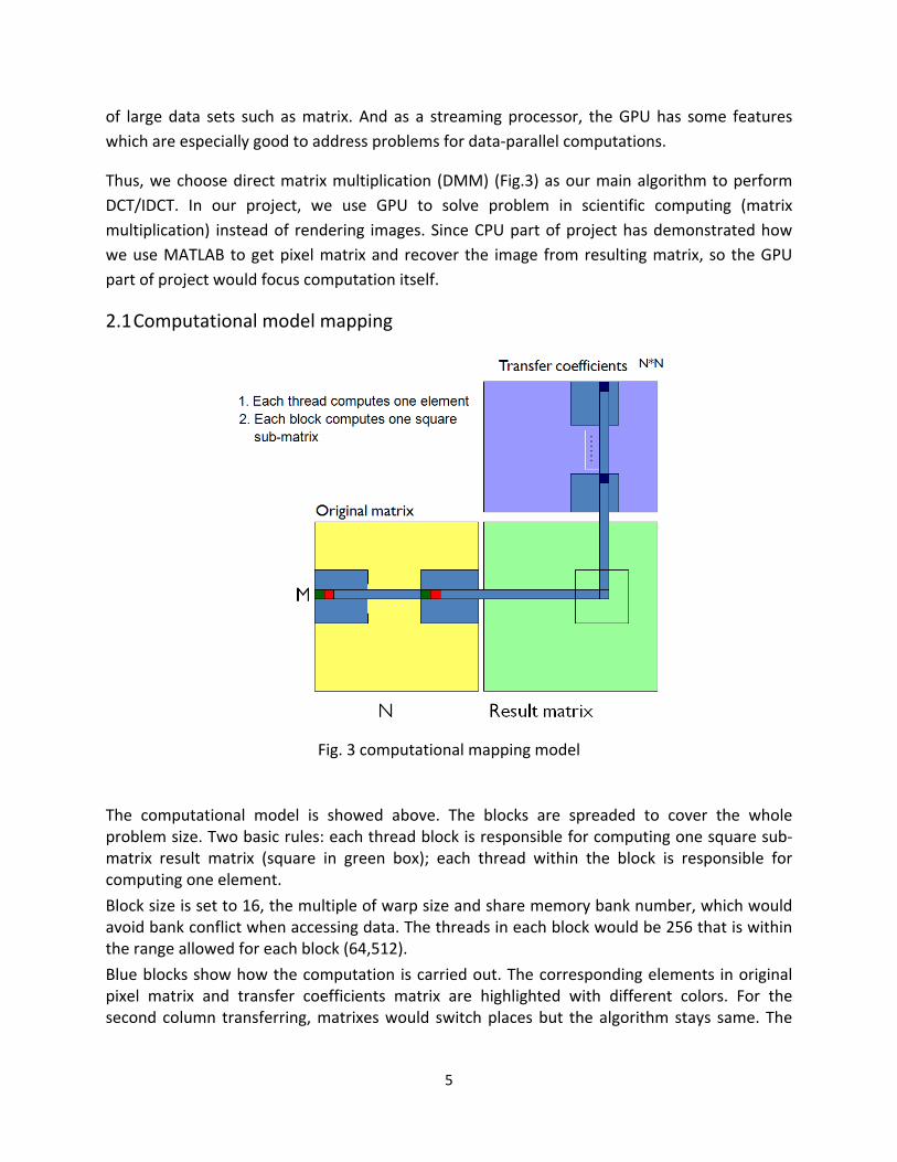
Thus, we choose direct matrix multiplication  (DMM)  (Fig.3) as our main algorithm to perform DCT/IDCT.  In  our  project,  we  use  GPU  to  solve  problem  in  scientific  computing  (matrix multiplication)  instead of rendering  images. Since CPU part of project has demonstrated how we use MATLAB  to get pixel matrix and recover  the  image  from resulting matrix, so  the GPU part of project would focus computation itself. 

2.1 Computational model mapping 

 

Fig. 3 computational mapping model 

 

The  computational  model  is  showed  above.  The  blocks  are  spreaded  to  cover  the  whole problem size. Two basic rules: each thread block is responsible for computing one square sub‐matrix  result matrix  (square  in  green  box);  each  thread within  the  block  is  responsible  for computing one element. 

Block size is set to 16, the multiple of warp size and share memory bank number, which would avoid bank conflict when accessing data. The threads in each block would be 256 that is within the range allowed for each block (64,512). 

Blue blocks show how the computation  is carried out. The corresponding elements  in original pixel  matrix  and  transfer  coefficients  matrix  are  highlighted  with  different  colors.  For  the second column  transferring, matrixes would  switch places but  the algorithm  stays  same. The 

6  

registers would accumulate the value from each multiplication till the loop finishes the width of original matrix. 

 

2.2  Memory model and usage 

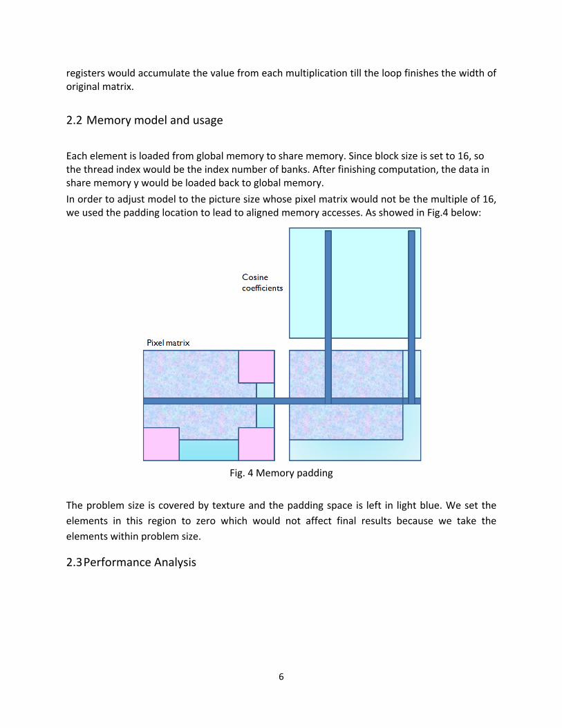
 Each element is loaded from global memory to share memory. Since block size is set to 16, so the thread index would be the index number of banks. After finishing computation, the data in share memory y would be loaded back to global memory. In order to adjust model to the picture size whose pixel matrix would not be the multiple of 16, we used the padding location to lead to aligned memory accesses. As showed in Fig.4 below: 

 Fig. 4 Memory padding  

 

The problem size  is covered by texture and the padding space  is  left  in  light blue. We set the elements  in  this  region  to  zero  which  would  not  affect  final  results  because  we  take  the elements within problem size. 

2.3 Performance Analysis 

7  

  

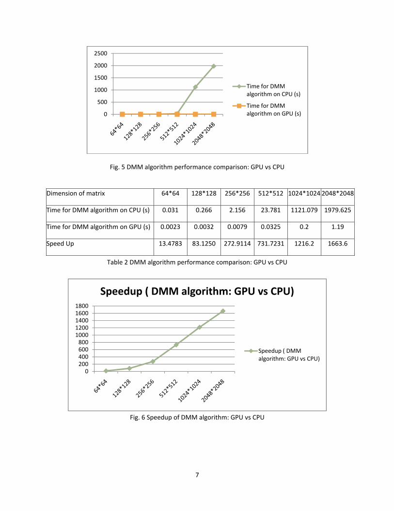
Fig. 5 DMM algorithm performance comparison: GPU vs CPU   

Dimension of matrix  64*64  128*128  256*256  512*512  1024*1024 2048*2048

Time for DMM algorithm on CPU (s)  0.031  0.266  2.156  23.781  1121.079 1979.625

Time for DMM algorithm on GPU (s)  0.0023  0.0032  0.0079  0.0325  0.2  1.19 

Speed Up  13.4783  83.1250  272.9114 731.7231  1216.2  1663.6 

Table 2 DMM algorithm performance comparison: GPU vs CPU 

 

 Fig. 6 Speedup of DMM algorithm: GPU vs CPU 

 

 

0

500

1000

1500

2000

2500

Time for DMM algorithm on CPU (s)

Time for DMM algorithm on GPU (s)

020040060080010001200140016001800

Speedup ( DMM algorithm: GPU vs CPU)

Speedup ( DMM algorithm: GPU vs CPU)

8  

The time consumed by CPU program increases “exponentially” as the dimension of matrix goes up, while GPU uses much less time especially for large matrix (see the last row of speedup). We also  noticed  for  small  size  of matrix,  CPU works  better.  This will  not  undermine  our  efforts because the only  large matrix computation needs GPU to speed up while the application only involves small size of picture does not have to go through all the trouble of GPU.  In order to understand this problem better, we examine the efficiency of different parts of code. The major parts  could  be  divided  into  coefficient  generation  (kernel:Cof_generator())  and  matrix multiplication (kernel: mul()). Below cylinder diagram showed the time consumed by these two parts separately.  Furthermore,  we  found  that  the  time  for  coefficient  generator  increases  with  dimensions slowly, basically keeps the same amount time. While matrix multiplication takes more time for large matrix. So optimization discussed below would be addressed these two parts. For small matrix, the optimization on coefficient generator routine makes more sense, while optimization for large matrix would make a difference on performance.  

2.4 Optimization of coefficient generator 

Only 2*N different cosine elements involved, we can use the same optimization in CPU part to avoid repeating calculation. 

Ds[ty][tx] = sqrt((double)2/N)*cos[(2*Py+1)*Px*Pi/(2*N)]; 

Therefore, the complexity of problem is reduced: O(N*N)‐‐O(N). 

As we  learned  from  class,  using  constant memory  for  parameters  used  frequently  in  code would improve the performance. 

Ds[ty][tx] = sqrt((double)2/N) * myConstantArray[(2*Py+1)*Px%(4*N)]; 

 

2.5 Optimization of matrix multiplication 

At first stage, we use the clear implementation to make sure code runs correctly. After checking results matrix with those of CPU, we can move to next step to make it more efficient. 

Fortunately, the last few lectures introduced some techniques that can apply to our problems. 

a) Pre‐fetch data 

To avoid reading address of matrix, registers are used to speed up the access of data. The ideas are illustrated in below code part (only the related part). 

float Atemp=A[a + wA1 * ty + tx]; 

9  

float Btemp=B[b + wB1 * ty + tx]; 

// Shared memory for the sub‐matrix of A 

__shared__ float As[BLOCK_SIZE][BLOCK_SIZE]; 

//Shared memory for the sub‐matrix of B 

__shared__ float Bs[BLOCK_SIZE][BLOCK_SIZE]; 

// Load the matrices from global memory to //shared memory; 

// each thread loads one element of each //matrix 

As[ty][tx] = Atemp; 

Bs[ty][tx] = Btemp; 

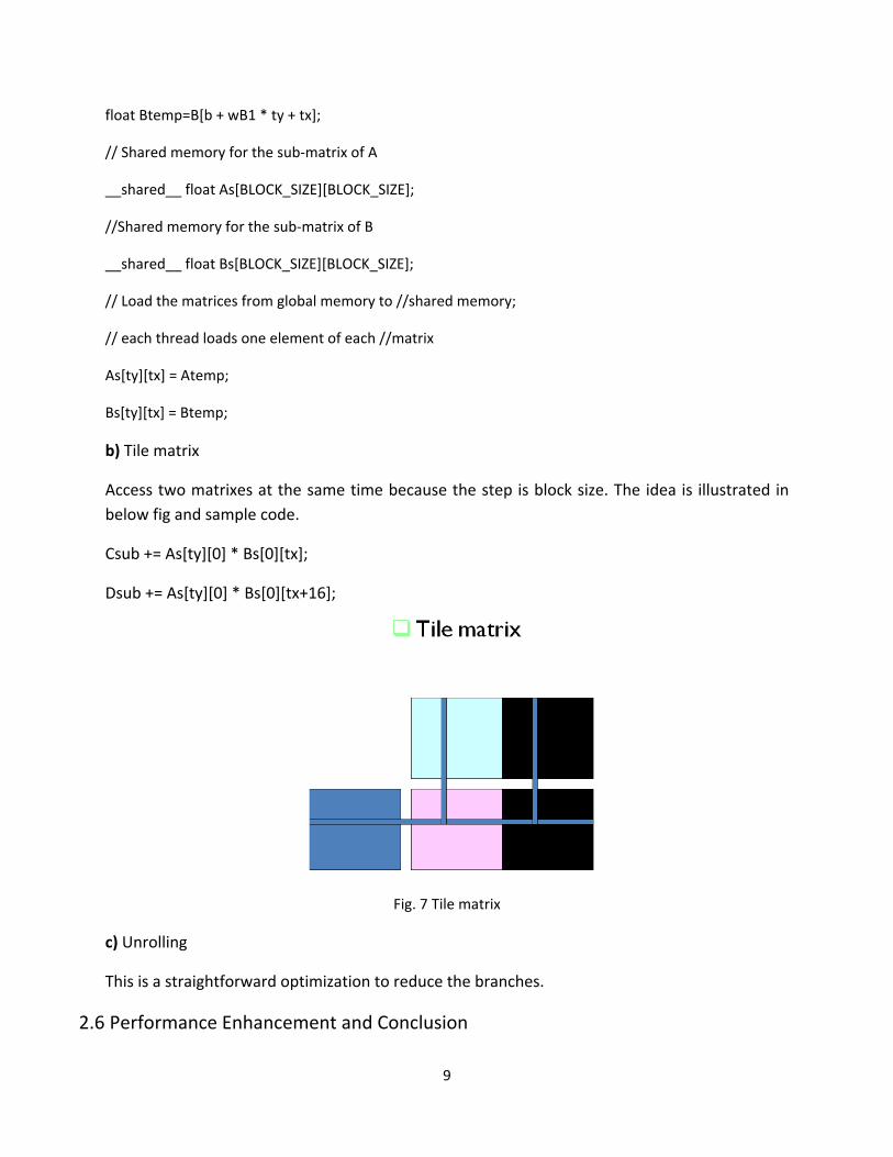
b) Tile matrix 

Access two matrixes at the same time because the step  is block size. The  idea  is  illustrated  in below fig and sample code. 

Csub += As[ty][0] * Bs[0][tx]; 

Dsub += As[ty][0] * Bs[0][tx+16]; 

 

Fig. 7 Tile matrix 

c) Unrolling 

This is a straightforward optimization to reduce the branches. 

2.6 Performance Enhancement and Conclusion 

10  

The comparison of the direct matrix multiplication and optimized version is shown above.  

• The optimization for generating cosine coefficients did not contribute much • The  optimization  technique  used  for  matrix  multiplication  significantly  reduced 

computation time than previous version, especially for large matrix (highlighted in red).  

Conclusion: 

• Using appropriate compute and memory model to implement matrix multiplication on GPU will greatly speed up computation. 

• To make  the better use of computation  resources,  the optimization  techniques are used, and the enhanced performances are demonstrated  in the comparison table.  It shows that the  bits  of  techniques  are  worth  of  learning  because  they  would  contribute  to  better performance with same resources. 

 

   

 

1. Algo

1.1 The 

Firstly, le

 N 

2 

Comparin

 

From theDFT. AndAs for thpart, we After anaand  FFTperformabelow (n

orithm de

relationsh

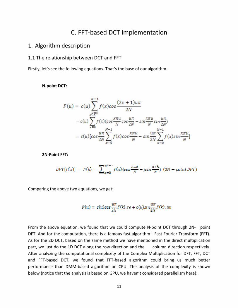
et’s see the f

N‐point DCT:

N‐Point FFT

ng the above

e above equd for the come 2D DCT, bjust do the alyzing the cT‐based  DCTance  than  Dotice that th

C. FFT‐

escription

hip betwee

following eq

  

T: 

e two equat

uation, we  fomputation, tbased on the1D DCT alocomputationT,  we  founDMM‐basedhe analysis is

‐based D

n 

en DCT and

uations. Tha

tions, we get

ound that wthere is a fae same methng the row nal complexnd  that  FFT  algorithm s based on G

11 

DCT impl

d FFT 

at’s the base

 

 

t: 

 

we could commous fast ahod we havedirection anity of the CoT‐based  algon  CPU.  ThGPU, we hav

ementa

e of our algo

mpute N‐poalgorithm—Fe mentionednd the      coomplex Mulgorithm  couhe  analysis en’t conside

tion 

rithm. 

 

oint DCT throFast Fourier d in the direolumn directtiplication fuld  bring  uof  the  comered parallel

 

 

ough 2N‐     Transform (ect multipliction respector DFT, FFT,us  much  bplexity  is  shism here): 

point (FFT). ation ively. , DCT better hown 

12  

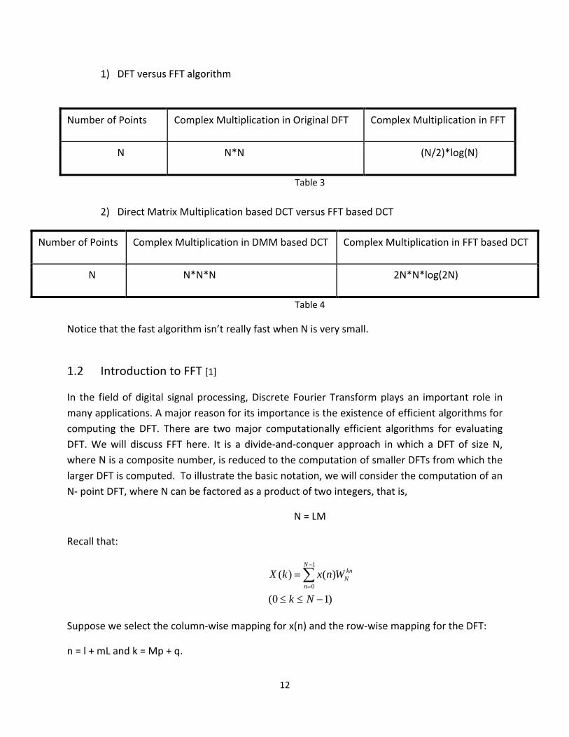
1) DFT versus FFT algorithm  

Number of Points  Complex Multiplication in Original DFT Complex Multiplication in FFT

N  N*N (N/2)*log(N)

Table 3  

2) Direct Matrix Multiplication based DCT versus FFT based DCT 

Number of Points  Complex Multiplication in DMM based DCT  Complex Multiplication in FFT based DCT 

N  N*N*N  2N*N*log(2N)

Table 4 

Notice that the fast algorithm isn’t really fast when N is very small. 

 

1.2 Introduction to FFT [1] 

In  the  field of digital  signal processing, Discrete Fourier Transform plays an  important  role  in many applications. A major reason for its importance is the existence of efficient algorithms for computing  the DFT.  There  are  two major  computationally efficient  algorithms  for evaluating DFT. We will discuss FFT here.  It  is a divide‐and‐conquer approach  in which a DFT of  size N, where N is a composite number, is reduced to the computation of smaller DFTs from which the larger DFT is computed.  To illustrate the basic notation, we will consider the computation of an N‐ point DFT, where N can be factored as a product of two integers, that is, 

N = LM 

Recall that: 

 

1

0( ) ( )

(0 1)

Nkn

Nn

X k x n W

k N

−

=

=

≤ ≤ −

∑  

Suppose we select the column‐wise mapping for x(n) and the row‐wise mapping for the DFT:  

n = l + mL and k = Mp + q.  

13  

 

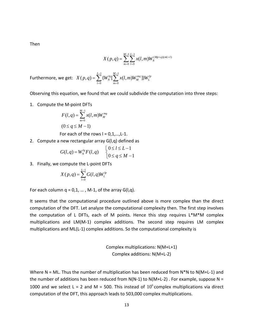
Then 

1 1( )( )

0 0( , ) ( , )

M LMp q mL l

Nm l

X p q x l m W− −

+ +

= =

= ∑∑  

Furthermore, we get:  1 1

0 0( , ) { [ ( , ) ]}

L Mlq mq lp

N M Ll m

X p q W x l m W W− −

= =

= ∑ ∑  

Observing this equation, we found that we could subdivide the computation into three steps: 

1. Compute the M‐point DFTs 

 

1

0( , ) ( , )

(0 1)

Mmq

Mm

F l q x l m W

q M

−

=

=

≤ ≤ −

∑  

For each of the rows l = 0,1,…,L‐1. 2. Compute a new rectangular array G(l,q) defined as 

0 1( , ) ( , )

0 1lq

N

l LG l q W F l q

q M≤ ≤ −⎧

= ⎨ ≤ ≤ −⎩ 

3. Finally, we compute the L‐point DFTs 1

0( , ) ( , )

Llp

Ll

X p q G l q W−

=

= ∑  

For each column q = 0,1, … , M‐1, of the array G(l,q). 

It  seems  that  the  computational procedure outlined  above  is more  complex  than  the direct computation of the DFT. Let analyze the computational complexity then. The first step involves the  computation  of  L  DFTs,  each  of  M  points.  Hence  this  step  requires  L*M*M  complex multiplications  and  LM(M‐1)  complex  additions.  The  second  step  requires  LM  complex multiplications and ML(L‐1) complex additions. So the computational complexity is  

 Complex multiplications: N(M+L+1) 

Complex additions: N(M+L‐2)  

Where N = ML. Thus the number of multiplication has been reduced from N*N to N(M+L‐1) and the number of additions has been reduced from N(N‐1) to N(M+L‐2) . For example, suppose N = 

1000 and we  select L = 2 and M = 500. This  instead of  610 complex multiplications via direct computation of the DFT, this approach leads to 503,000 complex multiplications. 

14  

    

When    N  is  a  highly  composite  number,  that  is,  N  can  be  factored  into  product  of  prime 

numbers of the  form  1 2 vN r r r=  then the decomposition above can be repeated  (v‐1) more 

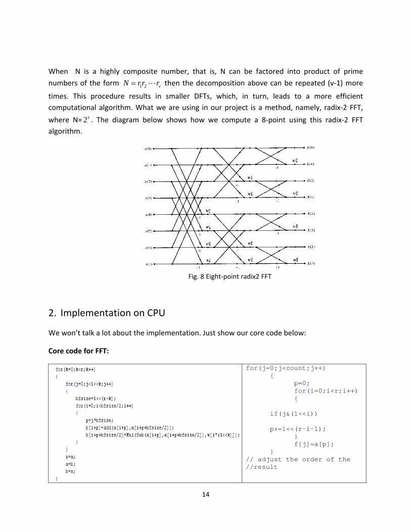
times.  This  procedure  results  in  smaller  DFTs,  which,  in  turn,  leads  to  a  more  efficient computational algorithm. What we are using  in our project  is a method, namely, radix‐2 FFT, 

where  N= 2v .  The  diagram  below  shows  how we  compute  a  8‐point  using  this  radix‐2  FFT algorithm. 

 Fig. 8 Eight‐point radix2 FFT 

 

2. Implementation on CPU 

We won’t talk a lot about the implementation. Just show our core code below: 

Core code for FFT: 

for(j=0;j<count;j++) { p=0; for(i=0;i<r;i++) { if(j&(1<<i)) p+=1<<(r-i-1); } f[j]=a[p]; } // adjust the order of the //result  

15  

 

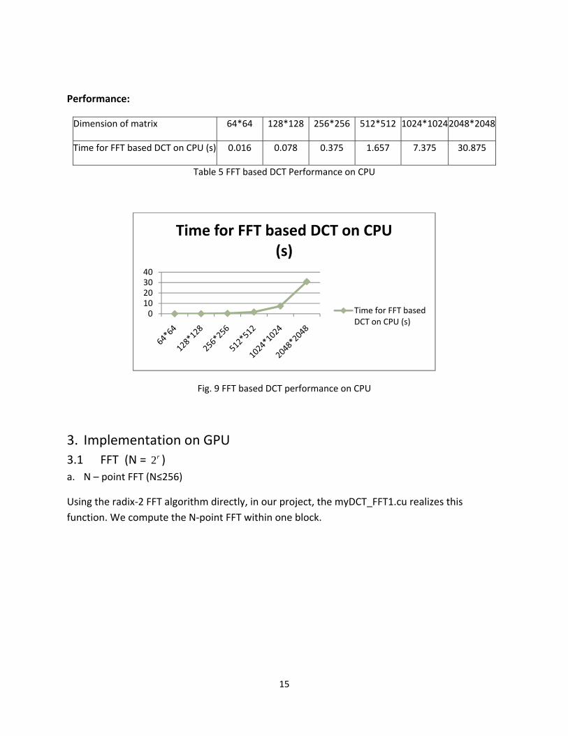
Performance: 

Dimension of matrix  64*64  128*128 256*256 512*512 1024*1024 2048*2048

Time for FFT based DCT on CPU (s)  0.016  0.078  0.375  1.657  7.375  30.875 

Table 5 FFT based DCT Performance on CPU 

 

 

Fig. 9 FFT based DCT performance on CPU 

 

3. Implementation on GPU 3.1 FFT  (N =  2r ) a. N – point FFT (N≤256) 

Using the radix‐2 FFT algorithm directly, in our project, the myDCT_FFT1.cu realizes this function. We compute the N‐point FFT within one block.  

 

010203040

Time for FFT based DCT on CPU (s)

Time for FFT based DCT on CPU (s)

16  

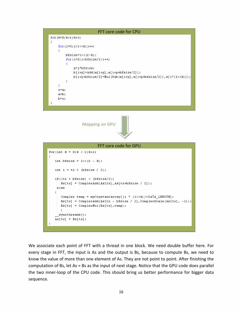
FFT core code for CPU  

 

                                                  

                                                  Mapping on GPU 

 

FFT core code for GPU 

  

 

We associate each point of FFT with a  thread  in one block. We need double buffer here. For      every stage  in FFT,  the  input  is As and  the output  is Bs, because  to compute Bs, we need  to know the value of more than one element of As. They are not point to point. After finishing the computation of Bs, let As = Bs as the input of next stage. Notice that the GPU code does parallel the  two  inner‐loop of  the CPU code. This should bring us better performance  for bigger data sequence. 

17  

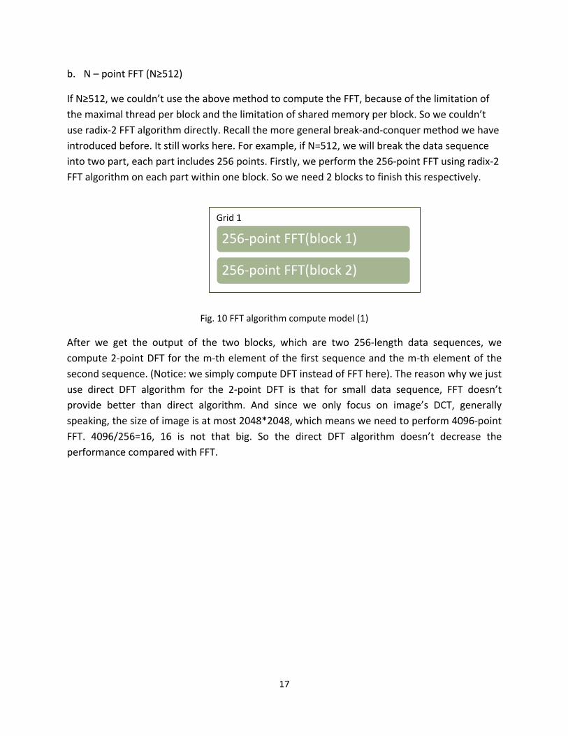
b. N – point FFT (N≥512) 

If N≥512, we couldn’t use the above method to compute the FFT, because of the limitation of the maximal thread per block and the limitation of shared memory per block. So we couldn’t use radix‐2 FFT algorithm directly. Recall the more general break‐and‐conquer method we have introduced before. It still works here. For example, if N=512, we will break the data sequence into two part, each part includes 256 points. Firstly, we perform the 256‐point FFT using radix‐2 FFT algorithm on each part within one block. So we need 2 blocks to finish this respectively.  

 

 

 

Fig. 10 FFT algorithm compute model (1) 

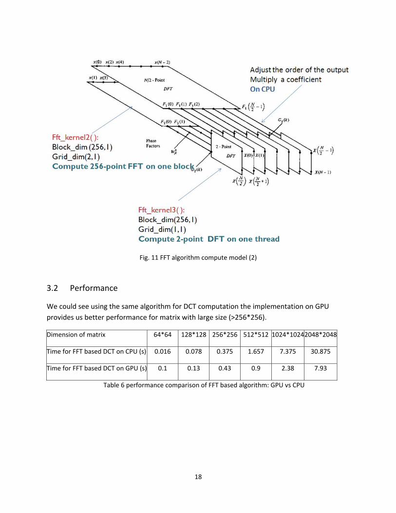
After we  get  the  output  of  the  two  blocks, which  are  two  256‐length  data  sequences, we compute 2‐point DFT for the m‐th element of the first sequence and the m‐th element of the second sequence. (Notice: we simply compute DFT instead of FFT here). The reason why we just use  direct  DFT  algorithm  for  the  2‐point  DFT  is  that  for  small  data  sequence,  FFT  doesn’t provide  better  than  direct  algorithm.  And  since  we  only  focus  on  image’s  DCT,  generally speaking, the size of image is at most 2048*2048, which means we need to perform 4096‐point FFT.  4096/256=16,  16  is  not  that  big.  So  the  direct  DFT  algorithm  doesn’t  decrease  the performance compared with FFT.  

256‐point FFT(block 2)

256‐point FFT(block 1) 

Grid 1 

18  

 

Fig. 11 FFT algorithm compute model (2) 

 3.2 Performance 

We could see using the same algorithm for DCT computation the implementation on GPU provides us better performance for matrix with large size (>256*256).  

Dimension of matrix  64*64  128*128 256*256 512*512 1024*10242048*2048

Time for FFT based DCT on CPU (s)  0.016  0.078  0.375  1.657  7.375  30.875 

Time for FFT based DCT on GPU (s) 0.1  0.13  0.43  0.9  2.38  7.93 

Table 6 performance comparison of FFT based algorithm: GPU vs CPU 

 

19  

 Fig. 12 Performance comparison for FFT based algorithm: GPU vs CPU 

Speedup 

 

Fig. 13 Speedup for FFT based algorithm: GPU vs CPU 

 

3.3 Optimization 

The only optimization we do  for  this  FFT‐based  algorithm  is using  constant  to  store  the  FFT coefficients  instead of download the coefficients  in global  to shared memory to perform FFT. But  the  performances of  the  two methods  are  almost  the  same.  So we won’t  discuss more about this issue. 

 

 

0

5

10

15

20

25

30

35

Time for FFT based DCT on CPU (s)

Time for FFT based DCT on GPU (s)

0

1

2

3

4

5

Speed up ( FFT based algorithm: GPU vs CPU)

Speedup ( FFT based algorithm: GPU vs CPU)

20  

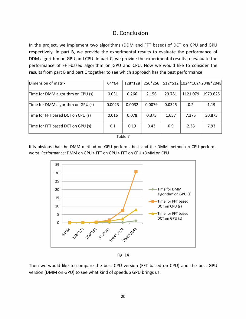
D. Conclusion 

In  the project, we  implement  two algorithms  (DDM and FFT based) of DCT on CPU and GPU respectively.  In  part B, we  provide  the  experimental  results  to  evaluate  the  performance  of DDM algorithm on GPU and CPU. In part C, we provide the experimental results to evaluate the performance  of  FFT‐based  algorithm  on GPU  and  CPU. Now we would  like  to  consider  the results from part B and part C together to see which approach has the best performance. 

Dimension of matrix  64*64  128*128 256*256 512*512  1024*10242048*2048

Time for DMM algorithm on CPU (s)  0.031  0.266  2.156  23.781  1121.079 1979.625

Time for DMM algorithm on GPU (s)  0.0023  0.0032  0.0079  0.0325  0.2  1.19 

Time for FFT based DCT on CPU (s)  0.016  0.078  0.375  1.657  7.375  30.875 

Time for FFT based DCT on GPU (s)  0.1  0.13  0.43  0.9  2.38  7.93 

Table 7  

It  is obvious  that  the DMM method on GPU performs best  and  the DMM method on CPU performs worst. Performance: DMM on GPU > FFT on GPU > FFT on CPU >DMM on CPU  

 

Fig. 14 

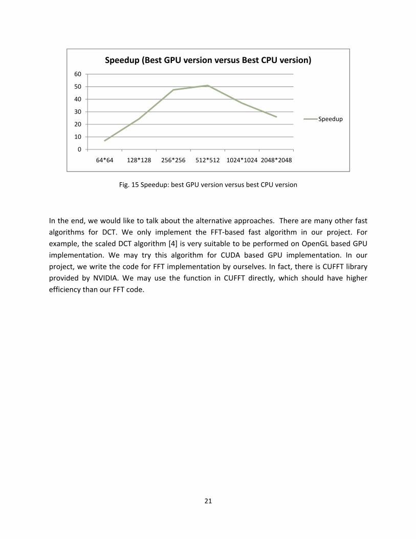
Then we would  like  to compare  the best CPU version  (FFT based on CPU) and  the best GPU version (DMM on GPU) to see what kind of speedup GPU brings us. 

0

5

10

15

20

25

30

35

Time for DMM algorithm on GPU (s)

Time for FFT based DCT on CPU (s)

Time for FFT based DCT on GPU (s)

21  

 

Fig. 15 Speedup: best GPU version versus best CPU version 

 

In the end, we would like to talk about the alternative approaches.  There are many other fast algorithms  for  DCT.  We  only  implement  the  FFT‐based  fast  algorithm  in  our  project.  For example, the scaled DCT algorithm [4] is very suitable to be performed on OpenGL based GPU implementation.  We  may  try  this  algorithm  for  CUDA  based  GPU  implementation.  In  our project, we write the code for FFT implementation by ourselves. In fact, there is CUFFT library provided  by NVIDIA. We may  use  the  function  in  CUFFT  directly, which  should  have  higher efficiency than our FFT code.  

 

0

10

20

30

40

50

60

64*64 128*128 256*256 512*512 1024*1024 2048*2048

Speedup (Best GPU version versus Best CPU version)

Speedup

22  

Reference: 

[1] John G. Proakis, Dimitris G. Monolakis, “Digital Signal Processing Principles, Algorithms, and Applications (Third Edition)” 

[2] “Application Note Discrete Cosine Transform with the LF3320” 

[3] “NVIDIA_CUDA_Programming_Guide_1.0” 

[4] Elliot Linzer, Ephraim Feig, “New scaled DCT algorithms for fused multiply/add architectures”