CSC 411: Lecture 09: Naive Bayes - University of Torontourtasun/courses/CSC411/09_naive_bayes… · CSC 411: Lecture 09: Naive Bayes Raquel Urtasun & Rich Zemel University of Toronto

CSC 411: Lecture 09: Naive Bayes

Raquel Urtasun & Rich Zemel

University of Toronto

Oct 9, 2015

Urtasun & Zemel (UofT) CSC 411: 09-Naive Bayes Oct 9, 2015 1 / 23

Today

Classification – Multi-dimensional Bayes classifier

Estimate probability densities from data

Naive Bayes


Generative vs Discriminative

Two approaches to classification:

Discriminative classifiers estimate parameters of decision boundary/classseparator directly from labeled sample

I learn boundary parameters directly (logistic regression models p(tk |x))I learn mappings from inputs to classes (least-squares, neural nets)

Generative approach: model the distribution of inputs characteristic of theclass (Bayes classifier)

I Build a model of p(x|tk)I Apply Bayes Rule


Bayes Classifier

Aim to diagnose whether patient has diabetes: classify into one of twoclasses (yes C=1; no C=0)

Run battery of tests

Given patient’s results: x = [x1, x2, · · · , xd ]T we want to update classprobabilities using Bayes Rule:

p(C |x) =p(x|C )p(C )

p(x)

More formally

posterior =Class likelihood× prior

Evidence

How can we compute p(x) for the two class case?

p(x) = p(x|C = 0)p(C = 0) + p(x|C = 1)p(C = 1)


Classification: Diabetes Example

Last class we had a single input/observation per patient: white blood cellcount

p(C = 1|x = 50) =p(x = 50|C = 1)p(C = 1)

p(x = 50)

Add second observation: Plasma glucose value

Can construct bivariate normal (Gaussian) distribution of each class


Gaussian Bayes Classifier

Gaussian (or normal) distribution:

p(x|t = k) =1

(2π)d/2|Σ|1/2exp

[−(x− µk)TΣ−1(x− µk)

]

Each class k has associated mean vector, but typically the classes share asingle covariance matrix


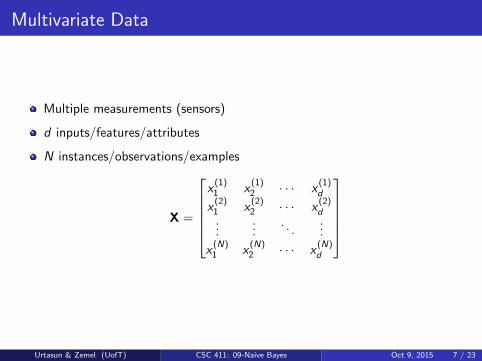
Multivariate Data

Multiple measurements (sensors)

d inputs/features/attributes

N instances/observations/examples

X =

x(1)1 x

(1)2 · · · x

(1)d

x(2)1 x

(2)2 · · · x

(2)d

......

. . ....

x(N)1 x

(N)2 · · · x

(N)d


Multivariate Parameters

MeanE[x] = [µ1, · · · , µd ]T

Covariance

Σ = Cov(x) = E[(x− µ)T (x− µ)] =

σ21 σ12 · · · σ1d

σ12 σ22 · · · σ2d

......

. . ....

σd1 σd2 · · · σ2d

Correlation = Corr(x) is the covariance divided by the product of standarddeviation

ρij =σijσiσj


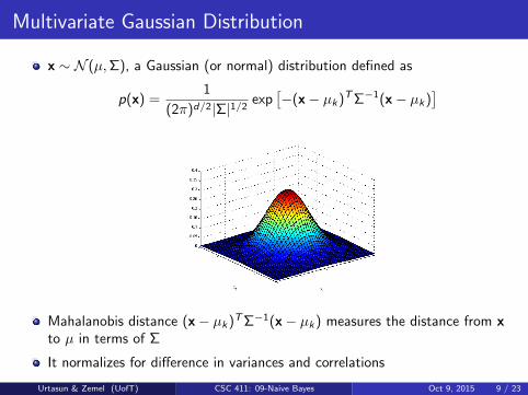
Multivariate Gaussian Distribution

x ∼ N (µ,Σ), a Gaussian (or normal) distribution defined as

p(x) =1

(2π)d/2|Σ|1/2exp

[−(x− µk)TΣ−1(x− µk)

]

Mahalanobis distance (x− µk)TΣ−1(x− µk) measures the distance from xto µ in terms of Σ

It normalizes for difference in variances and correlations


Bivariate Normal


Bivariate Normal


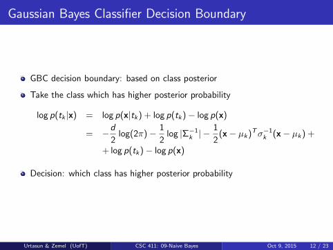
Gaussian Bayes Classifier Decision Boundary

GBC decision boundary: based on class posterior

Take the class which has higher posterior probability

log p(tk |x) = log p(x|tk) + log p(tk)− log p(x)

= −d

2log(2π)− 1

2log |Σ−1

k | −1

2(x− µk)Tσ−1

k (x− µk) +

+ log p(tk)− log p(x)

Decision: which class has higher posterior probability


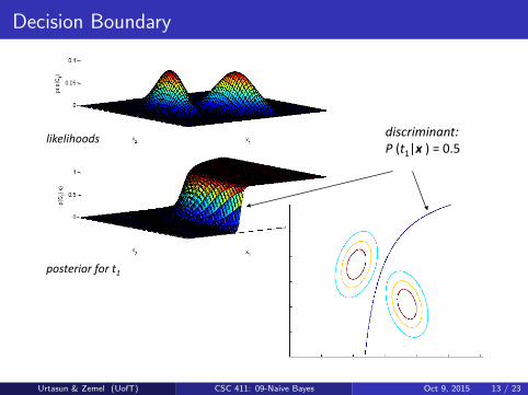
Decision Boundary

likelihoods)

posterior)for)t1)

discriminant:!!P!(t1|x")!=!0.5!


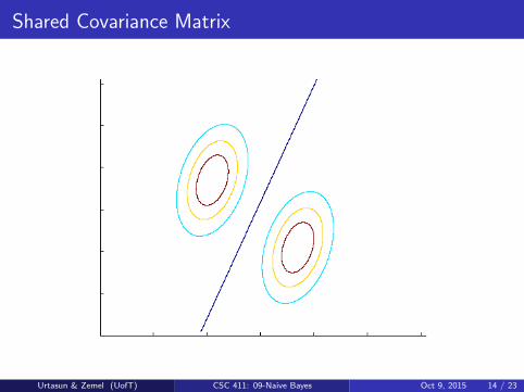
Shared Covariance Matrix


Learning Gaussian Bayes Classifier

Learn the parameters using maximum likelihood

`(φ, µ0, µ1,Σ) = − logN∏

n=1

p(x(n), t(n)|φ, µ0, µ1,Σ)

= − logN∏

n=1

p(x(n)|t(n), µ0, µ1,Σ)p(t(n)|φ)

What have I assumed?


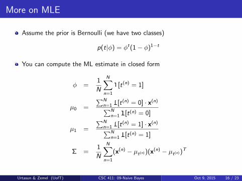
More on MLE

Assume the prior is Bernoulli (we have two classes)

p(t|φ) = φt(1− φ)1−t

You can compute the ML estimate in closed form

φ =1

N

N∑n=1

1[t(n) = 1]

µ0 =

∑Nn=1 1[t(n) = 0] · x(n)∑N

n=1 1[t(n) = 0]

µ1 =

∑Nn=1 1[t(n) = 1] · x(n)∑N

n=1 1[t(n) = 1]

Σ =1

N

N∑n=1

(x(n) − µt(n))(x(n) − µt(n))T


Naive Bayes

For Gaussian Bayes Classifier, if input x is high-dimensional, then covariancematrix has many parameters

Save some parameters by using a shared covariance for the classes

Naive Bayes is an alternative Generative model: assumes featuresindependent given the class

p(x|t = k) =d∏

i=1

p(xi |t = k)

How many parameters required now? And before?


Diagonal Covariance

variances may be different


Diagonal Covariance, isotropic

* ?

Classification only depends on distance to the mean


Naive Bayes Classifier

Given

prior

assuming features are conditionally independent given the class

likelihood for each xi

The decision rule

y = arg maxk

p(t = k)d∏

i=1

p(xi |t = k)

If the assumption of conditional independence holds, NB is the optimalclassifier

If not, a heavily regularized version of generative classifier

What’s the regularization?


Gaussian Naive Bayes

Assume

p(xi |t = k) =1√

2πσikexp

[−(xi − µik)2

2σ2ik

]

Maximum likelihood estimate of parameters

µik =

∑Nn=1 1[t(n) = k] · x (n)i∑N

n=1 1[t(n) = k]

Similar for the variance


Gaussian Bayes Classifier (GBC) vs Logistic Regression

If you examine p(t = 1|x) under GBC, you will find that it looks like this:

p(t|x, φ, µ0, µ1,Σ) =1

1 + exp(−w(φ, µ0, µ1,Σ)Tx)

So the decision boundary has the same form as logistic regression!

When should we prefer GBC to LR, and vice versa?


GBC vs LR

GBC makes stronger modeling assumption: assumes class-conditional data ismultivariate Gaussian

If this is true, GBC is asymptotically efficient (best model in limit of large N)

But LR is more robust, less sensitive to incorrect modeling assumptions

Many class-conditional distributions lead to logistic classifier

When these distributions are non-Gaussian, in limit of large N, LR beats GBC


Documents

CSC 411: Lecture 09: Naive Bayes - University of Torontourtasun/courses/CSC411/09_naive_bayes… · CSC 411: Lecture 09: Naive Bayes Raquel Urtasun & Rich Zemel University of Toronto