CS221 Midterm Solutions Summer 2013

Overall the class did very well on what was decidedly a medium-hard midterm. The class average was a 72, which was above the predicted average of 70. One nice result is that the grade distribution had positive skew. The median was a 78, and a healthy 66% of the class scored above the mean (something to think about). The standard deviation was 20 points, a statistic that captures the long tail of scores that were below the mean. If you scored under a 50 please talk to us!

Figure 1: Grade distribution for the midterm.

If you want a re-grade, please return your midterm with a cover sheet explaining what went wrong. We reserve the right to re-grade your entire exam.

0

5

10

15

20

25

30

Num

ber o

f Stu

dent

s

Grade Range

CS221 Midterm – 2 –

Problem 1: Short Answer (15 points) Consider a grid maze in a world like the one pac-man lives in. Suppose the maze solver agent can take diagonal steps as well as steps in the N/S/E/W directions. Design a non zero admissible heuristic h. Specifically, suppose your solver is at (i, j), and the goal is at (igoal,jgoal). Either give an explicit formula for h(i,j), or describe how you would compute it efficiently.

There are a few heuristics that work for this problem. Two examples:

min(|igoal – i|, |jgoal – j|),

Euclidean distance.

You know that your opponent is actually running depth 2 minimax with a poor heuristic funciton, using the result 80% of the time, and moving randomly otherwise. Would it be better to model this agent using MiniMax or ExpectiMax?

Expectimax. If an agent is playing anything other than a perfect maximization algorithm you should use expectimax (think of pacman vs random agent).

True or False: At the end of the transition step (elapseTime), hidden markov model beliefs do not need to be normalized.

True. The update equation does not have a normalization constant. True or False: We have a bayes net where X is independent of Y given Z. It is possible the assumption will no longer hold when conditioning on additional evidence to other variables in the network. I.e. there can be a set of nodes W so that X is not independent of Y given Z and W.

True. The new nodes in W could form a “v” structure which allows information to flow.

True or False. If there was just a single particle in a particle filter it would still adequately incorporate observations.

False. Reweighting (the process that incorporates the observations) doesn’t work if there is only one particle. That particle, once weights are normalized always has weight one, regardless of observations. In fact particle filters with 1 particle don’t incorporate observations at all, particle filters several particles incorporate an approximation of the effect on belief and only as particles approach infinity do you perfectly incorporate observations.

CS221 Midterm – 3 –

Problem 2: Vertical Seam Carving (20 points) In this problem you will create a discrete search problem formulation to reduce the width of a picture without changing the dimensions of important regions.

Consider the original image (on the left). It we want to resize it to a smaller image (on the right) we could scale the image. However this would make the castle look distorted. The Vertical Seam Carving solution is to reduce the width of an image by repeating the process of removing the least important “seams” from a photo until the image is the desired width. A seam is a path of connected pixels from the top of the image to the bottom with exactly one pixel per row. A pixel is connected to its 8 direct neighbors.

The importance of a seam is the sum of the importance of its pixels. On the right the least important seams are visualized. Note that the least important seams do not cross the castle. Assume you are given the importance of each pixel

CS221 Midterm – 4 –

2a. Formalize the task of finding the least important vertical seam as a deterministic search problem (15 points). State Description:

Each state has a row and a col field.

Legal Actions (given a state):

Legal actions are going to be named by the col of the successor state. If the row is -1, aka you were in the start state, your action can be any col in the image. Else your legal actions are {state.col - 1, state.col or state.col + 1}

Successor (given a state and an action):

The successor row = state.row + 1. The successor col = action.col.

Cost (given a state and an action):

The importance of the pixel that corresponds to the current state. x = state.col y = state.row cost = importance(x, y).

Start State:

State.row = anything. State.col = -1

Terminal Test (given a state)

State.col is greater than the height of the image.

CS221 Midterm – 5 –

2b. Circle all of the algorithms that are guaranteed to find the least important seam, given your DFS formalization (3 points).

Breadth First Search Depth First Search A* with an Admissible Heuristic.

Technically you need a heuristic that is admissible AND consistent. We accepted all answers because there is a version of A* that works with only an admissible heuristic.

A* with an overestimating Heuristic Uniform Cost Search Bellman-Ford

2c. If your picture is 100 pixels high give a lower bound on the worst case number of nodes BFS would expand (2 points).

There were several correct answers. Also note, we changed the number of pixels for some exams to be 200 to make sure no-body took a cheeky peek at someone else’s test. Nobody did J.

1. Since searches keep a visited set, 100 * width is a lower bound. 2. If you run a search algorithm without a visited set and only check

terminal conditions once an element has been removed from the container: w*3100 (the w is for the first move).

3. If you run a search algorithm without a visited set and check terminal conditions when you generate successors: w*399 (the w is for the first move).

CS221 Midterm – 6 –

3. Lets Make a Deal (25 points) Solving a negotiation is a game theoretic situation similar to the adversarial search problems seen in pacman. In the negotiation “game” there are two agents and they take turns taking actions. One important distinction is that it is not a zero sum game. For each terminal state there are separate utilities for the two players that do not have to negate one another. Both agents can win. Both can lose. That’s life in the city.

Negotiation assumptions:

• The central assumption is that both agents in the negotiation only care about maximizing their own utility.

• We are also going to assume that the two players do not collude. In other words they do not decide together on a set of actions.

In this problem we will analyze how to make an optimal action for a negotiation game without zero sum rewards.

CS221 Midterm – 7 –

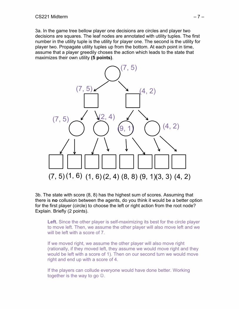
3a. In the game tree bellow player one decisions are circles and player two decisions are squares. The leaf nodes are annotated with utility tuples. The first number in the utility tuple is the utility for player one. The second is the utility for player two. Propagate utility tuples up from the bottom. At each point in time, assume that a player greedily choses the action which leads to the state that maximizes their own utility (5 points).

3b. The state with score (8, 8) has the highest sum of scores. Assuming that there is no collusion between the agents, do you think it would be a better option for the first player (circle) to choose the left or right action from the root node? Explain. Briefly (2 points).

Left. Since the other player is self-maximizing its best for the circle player to move left. Then, we assume the other player will also move left and we will be left with a score of 7. If we moved right, we assume the other player will also move right (rationally, if they moved left, they assume we would move right and they would be left with a score of 1). Then on our second turn we would move right and end up with a score of 4. If the players can collude everyone would have done better. Working together is the way to go J.

(7, 5)

(7, 5)

(7, 5)

(2, 4) (4, 2) (9, 1)

(4, 2)

CS221 Midterm – 8 –

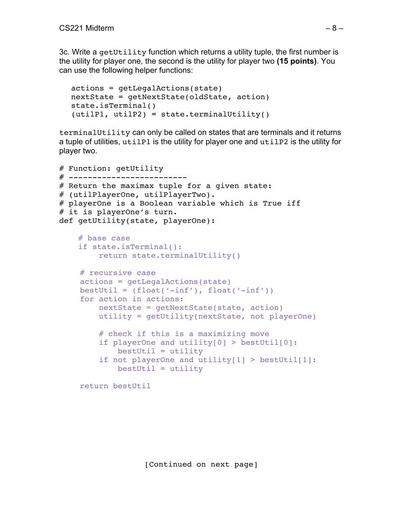
3c. Write a getUtility function which returns a utility tuple, the first number is the utility for player one, the second is the utility for player two (15 points). You can use the following helper functions:

actions = getLegalActions(state) nextState = getNextState(oldState, action) state.isTerminal() (utilP1, utilP2) = state.terminalUtility()

terminalUtility can only be called on states that are terminals and it returns a tuple of utilities, utilP1 is the utility for player one and utilP2 is the utility for player two. # Function: getUtility # ------------------------- # Return the maximax tuple for a given state: # (utilPlayerOne, utilPlayerTwo). # playerOne is a Boolean variable which is True iff # it is playerOne’s turn. def getUtility(state, playerOne): # base case if state.isTerminal():

return state.terminalUtility() # recursive case actions = getLegalActions(state) bestUtil = (float(‘-inf’), float(‘-inf’)) for action in actions: nextState = getNextState(state, action) utility = getUtility(nextState, not playerOne) # check if this is a maximizing move if playerOne and utility[0] > bestUtil[0]: bestUtil = utility if not playerOne and utility[1] > bestUtil[1]: bestUtil = utility return bestUtil

[Continued on next page]

CS221 Midterm – 9 –

3d. In minimax we were able to use alpha-beta pruning to eliminate some states from consideration. Would it be possible to prune states in this algorithm? Explain. Briefly (3 points).

No. Pruning does not work in this case. As a simple counter example, there could be a node with (infinity, infinity) utilities hidden anywhere in the tree. We must explore all nodes to find it.

CS221 Midterm – 10 –

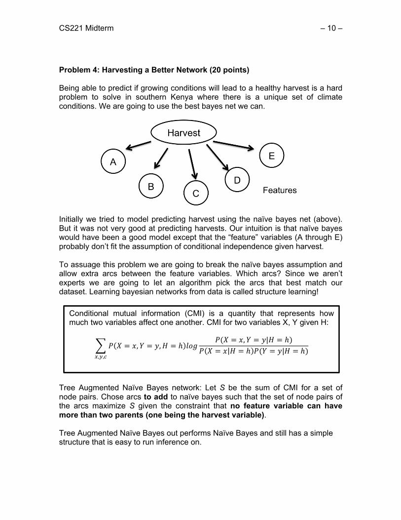
Problem 4: Harvesting a Better Network (20 points) Being able to predict if growing conditions will lead to a healthy harvest is a hard problem to solve in southern Kenya where there is a unique set of climate conditions. We are going to use the best bayes net we can.

Initially we tried to model predicting harvest using the naïve bayes net (above). But it was not very good at predicting harvests. Our intuition is that naïve bayes would have been a good model except that the “feature” variables (A through E) probably don’t fit the assumption of conditional independence given harvest. To assuage this problem we are going to break the naïve bayes assumption and allow extra arcs between the feature variables. Which arcs? Since we aren’t experts we are going to let an algorithm pick the arcs that best match our dataset. Learning bayesian networks from data is called structure learning!

Tree Augmented Naïve Bayes network: Let S be the sum of CMI for a set of node pairs. Chose arcs to add to naïve bayes such that the set of node pairs of the arcs maximize S given the constraint that no feature variable can have more than two parents (one being the harvest variable). Tree Augmented Naïve Bayes out performs Naïve Bayes and still has a simple structure that is easy to run inference on.

Conditional mutual information (CMI) is a quantity that represents how much two variables affect one another. CMI for two variables X, Y given H:

! 𝑃(𝑋 = 𝑥,𝑌 = 𝑦,𝐻 = ℎ)𝑙𝑜𝑔𝑃(𝑋 = 𝑥,𝑌 = 𝑦|𝐻 = ℎ)

𝑃(𝑋 = 𝑥|𝐻 = ℎ)𝑃(𝑌 = 𝑦|𝐻 = ℎ)!,!,!

CS221 Midterm – 11 –

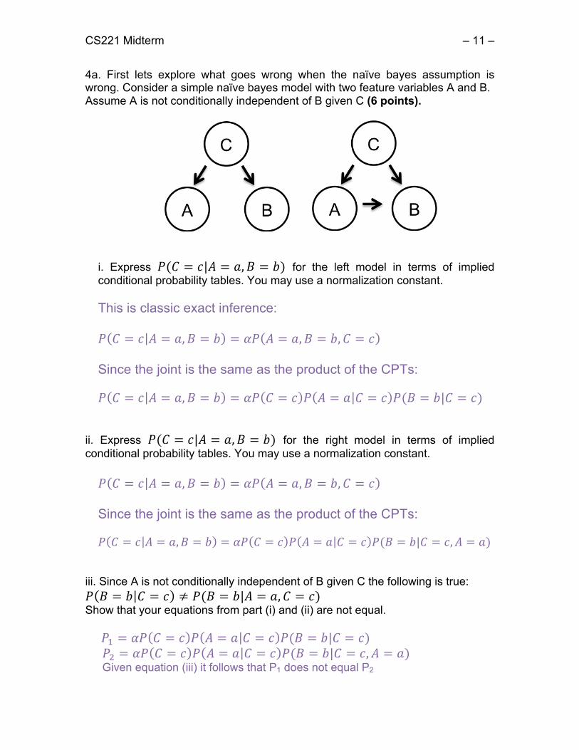
4a. First lets explore what goes wrong when the naïve bayes assumption is wrong. Consider a simple naïve bayes model with two feature variables A and B. Assume A is not conditionally independent of B given C (6 points).

i. Express 𝑃(𝐶 = 𝑐|𝐴 = 𝑎,𝐵 = 𝑏) for the left model in terms of implied conditional probability tables. You may use a normalization constant.

This is classic exact inference:

𝑃 𝐶 = 𝑐 𝐴 = 𝑎,𝐵 = 𝑏 = 𝛼𝑃 𝐴 = 𝑎,𝐵 = 𝑏,𝐶 = 𝑐 Since the joint is the same as the product of the CPTs:

𝑃 𝐶 = 𝑐 𝐴 = 𝑎,𝐵 = 𝑏 = 𝛼𝑃 𝐶 = 𝑐 𝑃 𝐴 = 𝑎 𝐶 = 𝑐 𝑃(𝐵 = 𝑏|𝐶 = 𝑐)

ii. Express 𝑃(𝐶 = 𝑐|𝐴 = 𝑎,𝐵 = 𝑏) for the right model in terms of implied conditional probability tables. You may use a normalization constant. 𝑃 𝐶 = 𝑐 𝐴 = 𝑎,𝐵 = 𝑏 = 𝛼𝑃 𝐴 = 𝑎,𝐵 = 𝑏,𝐶 = 𝑐 Since the joint is the same as the product of the CPTs:

𝑃 𝐶 = 𝑐 𝐴 = 𝑎,𝐵 = 𝑏 = 𝛼𝑃 𝐶 = 𝑐 𝑃 𝐴 = 𝑎 𝐶 = 𝑐 𝑃(𝐵 = 𝑏|𝐶 = 𝑐,𝐴 = 𝑎)

iii. Since A is not conditionally independent of B given C the following is true: 𝑃 𝐵 = 𝑏 𝐶 = 𝑐 ≠ 𝑃(𝐵 = 𝑏|𝐴 = 𝑎,𝐶 = 𝑐) Show that your equations from part (i) and (ii) are not equal.

𝑃! = 𝛼𝑃 𝐶 = 𝑐 𝑃 𝐴 = 𝑎 𝐶 = 𝑐 𝑃(𝐵 = 𝑏|𝐶 = 𝑐) 𝑃! = 𝛼𝑃 𝐶 = 𝑐 𝑃 𝐴 = 𝑎 𝐶 = 𝑐 𝑃(𝐵 = 𝑏|𝐶 = 𝑐,𝐴 = 𝑎) Given equation (iii) it follows that P1 does not equal P2

CS221 Midterm – 12 –

4b. Let’s augment our naïve bayes net! In order to learn the augmented naïve bayes network, we must compute the conditional mutual information (CMI) between each pair of features. Explain how we can compute the different parts of the mutual information equation using data. Be concise (6 points): 𝑃 𝑋 = 𝑥,𝑌 = 𝑦,𝐻 = ℎ

𝐶𝑜𝑢𝑛𝑡  𝑜𝑓  𝑡𝑖𝑚𝑒𝑠  𝑋 = 𝑥,𝑌 = 𝑦,𝐻 = ℎ𝑆𝑖𝑧𝑒  𝑜𝑓  𝑑𝑎𝑡𝑎𝑠𝑒𝑡

𝑃(𝑋 = 𝑥,𝑌 = 𝑦|𝐻 = ℎ)

𝐶𝑜𝑢𝑛𝑡  𝑜𝑓  𝑡𝑖𝑚𝑒𝑠  𝑋 = 𝑥,𝑌 = 𝑦,𝐻 = ℎ𝐶𝑜𝑢𝑛𝑡  𝑜𝑓  𝑡𝑖𝑚𝑒𝑠  𝐻 = ℎ

𝑃 𝑋 = 𝑥 𝐻 = ℎ

𝐶𝑜𝑢𝑛𝑡  𝑜𝑓  𝑡𝑖𝑚𝑒𝑠  𝑋 = 𝑥,𝐻 = ℎ𝐶𝑜𝑢𝑛𝑡  𝑜𝑓  𝑡𝑖𝑚𝑒𝑠  𝐻 = ℎ

𝑃(𝑌 = 𝑦|𝐻 = ℎ)

𝐶𝑜𝑢𝑛𝑡  𝑜𝑓  𝑡𝑖𝑚𝑒𝑠  𝑌 = 𝑦,𝐻 = ℎ𝐶𝑜𝑢𝑛𝑡  𝑜𝑓  𝑡𝑖𝑚𝑒𝑠  𝐻 = ℎ

4c. State at least one formalization method we have learned in class that you could use to model the problem of choosing arcs to add to our naïve bayes net. The chosen arcs should maximize the sum of mutual information S given the stated constraints. Do not formalize the problem (2 points).

We accepted weighted CSP, CSP, or some form of search problem. The best answer is weighted CSP.

CS221 Midterm – 13 –

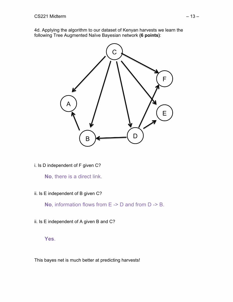
4d. Applying the algorithm to our dataset of Kenyan harvests we learn the following Tree Augmented Naïve Bayesian network (6 points):

i. Is D independent of F given C?

No, there is a direct link. ii. Is E independent of B given C?

No, information flows from E -> D and from D -> B.

ii. Is E independent of A given B and C?

Yes.

This bayes net is much better at predicting harvests!

CS221 Midterm – 14 –

Problem 5: Understanding Humans (20 points) A major milestone for building a strong AI agent—one whose intelligence is on par with human beings—is to teach a program to recognize emotion and personality. In the first part of the problem, we would like to track a single human’s emotion given an audio stream of the human talking. Then, given how their emotions change, we would like to guess at their personality type.

Figure: Humans are capable of a wide range of emotions J.

At each time slice, we observe a segment of sound from which we can extract the pitch contour—how the speaker’s pitch changes over the sound segment. Let the pitch contour at time t be Ct. The domain of pitch contour is {angular, glideUp, descending, flat, irregular}. We would like to know the emotion at each time slice Et. The domain of emotions is {sadness, surprise, joy, disgust, anger and fear}.

[Continued on next page]

CS221 Midterm – 15 –

5a. Formalize the task of tracking emotion using a Hidden Markov Model (6 points) What are the hidden variables?

Emotion at each time slice (Et) What are the observed variables?

Pitch Contour at each time slice (Ct)

What is the dimension of the transition conditional probability table?

6 x 6 = 36 What is the dimension of the emission conditional probability table?

5 x 6 = 30

What is a reasonable probability distribution for the hidden variable at time = 0?

Uniform distribution. (1/6) for each emotion.

CS221 Midterm – 16 –

5b. We want to know if the set of observations seem plausible given our emission and transition distributions. Write a formula to calculate the probability of seeing a particular sequence of observations over n time slices. Use probabilities from the conditional probability distributions implied by the hidden markov model. You can use a normalization constant. Note, this may include a huge sum. (7 points). 𝑃(𝐶! = 𝑐!,𝐶! = 𝑐!,…𝐶! = 𝑐!)

First, apply exact inference equation.

𝑃 𝐶! = 𝑐!,𝐶! = 𝑐!,…𝐶! = 𝑐! = 𝑃(𝐸 = 𝑒,𝐶 = 𝑐)!∈!

The joint can be expressed as the product of all the CPTs in the bayes net. 𝑃 𝐶! = 𝑐!,𝐶! = 𝑐!,…𝐶! = 𝑐! =

𝑃(𝐸! = 𝑒!)𝑃(𝐶! = 𝑐!|𝐸! = 𝑒!)!∈!

𝑃(𝐸! = 𝑒!|𝐸!!! = 𝑒!!!)𝑃(𝐶! = 𝑐!|𝐸! = 𝑒!)!

!!!

CS221 Midterm – 17 –

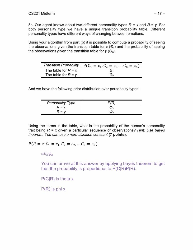
5c. Our agent knows about two different personality types R = x and R = y. For both personality type we have a unique transition probability table. Different personality types have different ways of changing between emotions. Using your algorithm from part (b) it is possible to compute a probability of seeing the observations given the transition table for x (Θx) and the probability of seeing the observations given the transition table for y (Θy).

Transition Probability P(C! = c!,C! = c!,… C! = c!) The table for R = x Θx The table for R = y Θy

And we have the following prior distribution over personality types:

Personality Type P(R) R = x Φx R = y Φy

Using the terms in the table, what is the probability of the human’s personality trait being R = x given a particular sequence of observations? Hint: Use bayes theorem. You can use a normalization constant (7 points). 𝑃(𝑅 = 𝑥|𝐶! = 𝑐!,𝐶! = 𝑐!,…𝐶! = 𝑐!)

𝛼𝜃!𝜙! You can arrive at this answer by applying bayes theorem to get that the probability is proportional to P(C|R)P(R). P(C|R) is theta x P(R) is phi x