CS 103 1

Tree Traversal Techniques; Heaps

• Tree Traversal Concept• Tree Traversal Techniques: Preorder,

Inorder, Postorder• Full Trees • Almost Complete Trees• Heaps

CS 103 2

Binary-Tree Related Definitions• The children of any node in a binary tree are

ordered into a left child and a right child• A node can have a left and

a right child, a left childonly, a right child only,or no children

• The tree made up of a leftchild (of a node x) and all itsdescendents is called the left subtree of x

• Right subtrees are defined similarly

10

1

3

11

98

4 6

5

7

12

CS 103 3

A Binary-tree Node Classclass TreeNode { public: typedef int datatype; TreeNode(datatype x=0, TreeNode *left=NULL,

TreeNode *right=NULL){data=x; this->left=left; this->right=right; };

datatype getData( ) {return data;};

TreeNode *getLeft( ) {return left;};

TreeNode *getRight( ) {return right;};void setData(datatype x) {data=x;};void setLeft(TreeNode *ptr) {left=ptr;};void setRight(TreeNode *ptr) {right=ptr;};

private:datatype data; // different data type for other appsTreeNode *left; // the pointer to left childTreeNode *right; // the pointer to right child

};

CS 103 4

Binary Tree Classclass Tree { public: typedef int datatype; Tree(TreeNode *rootPtr=NULL){this->rootPtr=rootPtr;}; TreeNode *search(datatype x); bool insert(datatype x); TreeNode * remove(datatype x); TreeNode *getRoot(){return rootPtr;}; Tree *getLeftSubtree(); Tree *getRightSubtree(); bool isEmpty(){return rootPtr == NULL;}; private: TreeNode *rootPtr;};

CS 103 5

Binary Tree Traversal

• Traversal is the process of visiting every node once

• Visiting a node entails doing some processing at that node, but when describing a traversal strategy, we need not concern ourselves with what that processing is

CS 103 6

Binary Tree Traversal Techniques

• Three recursive techniques for binary tree traversal

• In each technique, the left subtree is traversed recursively, the right subtree is traversed recursively, and the root is visited

• What distinguishes the techniques from one another is the order of those 3 tasks

CS 103 7

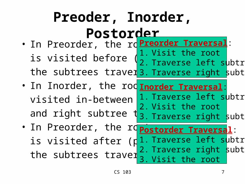
Preoder, Inorder, Postorder• In Preorder, the root

is visited before (pre)

the subtrees traversals• In Inorder, the root is

visited in-between left

and right subtree traversal• In Preorder, the root

is visited after (pre)

the subtrees traversals

Preorder Traversal:1. Visit the root2. Traverse left subtree3. Traverse right subtree

Inorder Traversal:1. Traverse left subtree2. Visit the root3. Traverse right subtree

Postorder Traversal:1. Traverse left subtree2. Traverse right subtree3. Visit the root

CS 103 8

Illustrations for Traversals• Assume: visiting a node

is printing its label• Preorder:

1 3 5 4 6 7 8 9 10 11 12• Inorder:

4 5 6 3 1 8 7 9 11 10 12• Postorder:

4 6 5 3 8 11 12 10 9 7 1

1

3

11

98

4 6

5

7

12

10

CS 103 9

Illustrations for Traversals (Contd.)

• Assume: visiting a node is printing its data

• Preorder: 15 8 2 6 3 711 10 12 14 20 27 22 30

• Inorder: 2 3 6 7 8 10 1112 14 15 20 22 27 30

• Postorder: 3 7 6 2 10 1412 11 8 22 30 27 20 15

6

158

2

3 7

11

10

14

12

20

27

22 30

CS 103 10

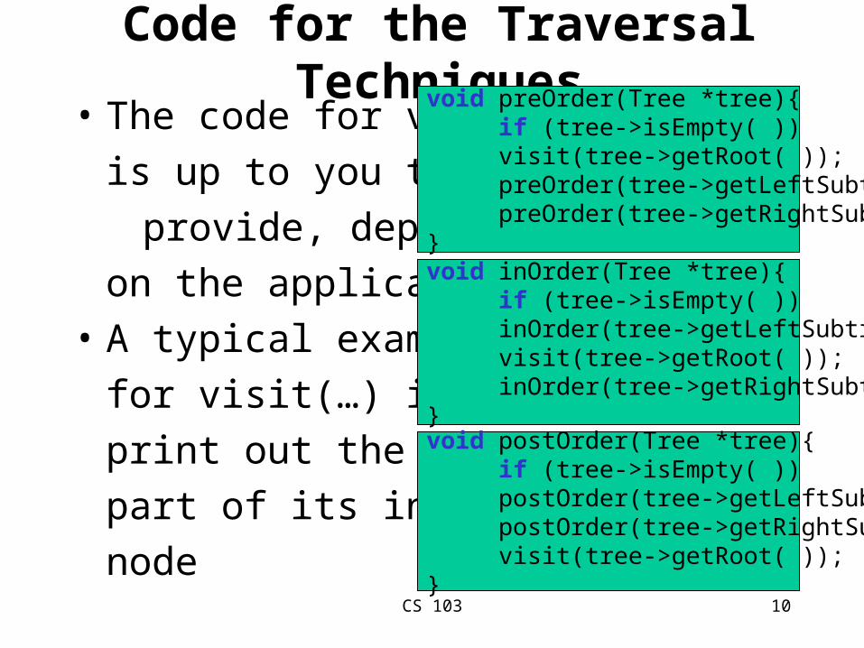
Code for the Traversal Techniques• The code for visit

is up to you to

provide, depending

on the application

• A typical example

for visit(…) is to

print out the data

part of its input

node

void inOrder(Tree *tree){ if (tree->isEmpty( )) return; inOrder(tree->getLeftSubtree( )); visit(tree->getRoot( )); inOrder(tree->getRightSubtree( ));}

void preOrder(Tree *tree){ if (tree->isEmpty( )) return; visit(tree->getRoot( )); preOrder(tree->getLeftSubtree()); preOrder(tree->getRightSubtree());}

void postOrder(Tree *tree){ if (tree->isEmpty( )) return; postOrder(tree->getLeftSubtree( )); postOrder(tree->getRightSubtree( )); visit(tree->getRoot( ));}

CS 103 11

Application of Traversal Sorting a BST

• Observe the output of the inorder traversal of the BST example two slides earlier

• It is sorted

• This is no coincidence

• As a general rule, if you output the keys (data) of the nodes of a BST using inorder traversal, the data comes out sorted in increasing order

CS 103 12

Other Kinds of Binary Trees(Full Binary Trees)

• Full Binary Tree: A full binary tree is a binary tree where all the leaves are on the same level and every non-leaf has two children

• The first four full binary trees are:

CS 103 13

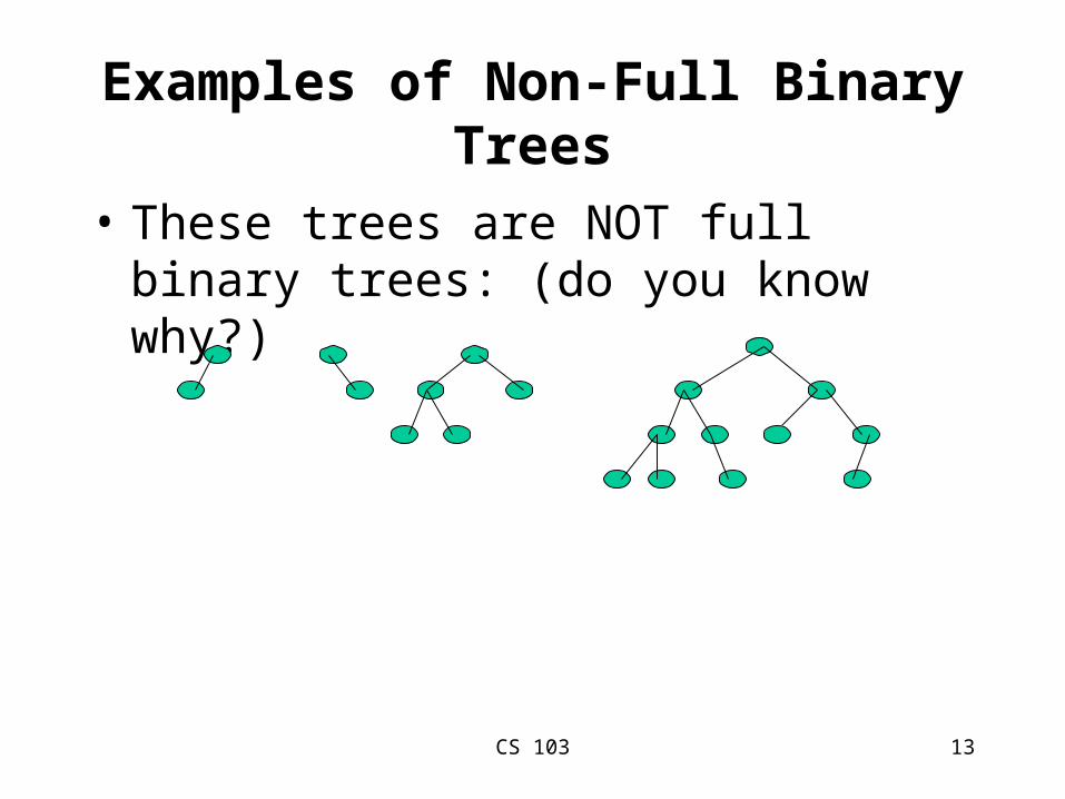
Examples of Non-Full Binary Trees

• These trees are NOT full binary trees: (do you know why?)

CS 103 14

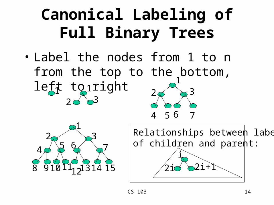
Canonical Labeling ofFull Binary Trees

• Label the nodes from 1 to n from the top to the bottom, left to right

1 1

2 3

12 3

4 5 6 71

2 3

4 5 6 7

8 9 10 111213 14 15

Relationships between labelsof children and parent:

2i 2i+1i

CS 103 15

Other Kinds of Binary Trees(Almost Complete Binary trees)

• Almost Complete Binary Tree: An almost complete binary tree of n nodes, for any arbitrary nonnegative integer n, is the binary tree made up of the first n nodes of a canonically labeled full binary

1 1

21

2 3

4 5 6 7

1

2

1

2 3

4 5 6

1

2 3

4

1

2 3

4 5

CS 103 16

Depth/Height of Full Trees and Almost Complete Trees

• The height (or depth ) h of such trees is O(log n)• Proof: In the case of full trees,

– The number of nodes n is: n=1+2+22+23+…+2h=2h+1-1

– Therefore, 2h+1 = n+1, and thus, h=log(n+1)-1

– Hence, h=O(log n)

• For almost complete trees, the proof is left as an exercise.

CS 103 17

Canonical Labeling ofAlmost Complete Binary Trees

• Same labeling inherited from full binary trees

• Same relationship holding between the labels of children and parents:

Relationships between labelsof children and parent:

2i 2i+1i

CS 103 18

Array Representation of Full Trees and Almost Complete Trees

• A canonically label-able tree, like full binary trees and almost complete binary trees, can be represented by an array A of the same length as the number of nodes

• A[k] is identified with node of label k• That is, A[k] holds the data of node k• Advantage:

– no need to store left and right pointers in the nodes save memory

– Direct access to nodes: to get to node k, access A[k]

CS 103 19

Illustration of Array Representation

• Notice: Left child of A[5] (of data 11) is A[2*5]=A[10] (of data 18),

and its right child is A[2*5+1]=A[11] (of data 12). • Parent of A[4] is A[4/2]=A[2], and parent of A[5]=A[5/2]=A[2]

6

158

2 11

18 12

20

27

13

30

15 8 20 2 11 30 27 13 6 10 121 2 3 4 5 6 7 8 9 10 11

CS 103 20

Adjustment of Indexes

• Notice that in the previous slides, the node labels start from 1, and so would the corresponding arrays

• But in C/C++, array indices start from 0• The best way to handle the mismatch is to adjust the

canonical labeling of full and almost complete trees.• Start the node labeling from 0 (rather than 1).• The children of node k are now nodes (2k+1) and

(2k+2), and the parent of node k is (k-1)/2, integer division.

CS 103 21

Application of Almost Complete Binary Trees: Heaps

• A heap (or min-heap to be precise) is an almost complete binary tree where– Every node holds a data value (or key)– The key of every node is ≤ the keys of the

children

Note:A max-heap has the same definition except that the Key of every node is >= the keys of the children

CS 103 22

Example of a Min-heap

16

5

8

15 11

18 12

20

27

33

30

CS 103 23

Operations on Heaps

• Delete the minimum value and return it. This operation is called deleteMin.

• Insert a new data value

Applications of Heaps:• A heap implements a priority queue, which is a queue that orders entities not a on first-come first-serve basis, but on a priority basis: the item of highest priority is at the head, and the item of the lowest priority is at the tail

• Another application: sorting, which will be seen later

CS 103 24

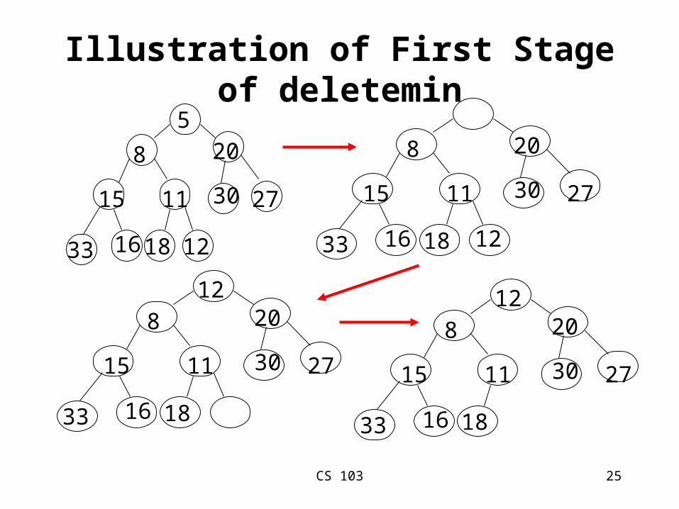
DeleteMin in Min-heaps

• The minimum value in a min-heap is at the root!• To delete the min, you can’t just remove the data

value of the root, because every node must hold a key

• Instead, take the last node from the heap, move its key to the root, and delete that last node

• But now, the tree is no longer a heap (still almost complete, but the root key value may no longer be ≤ the keys of its children

CS 103 25

Illustration of First Stage of deletemin

16

5

8

15 11

18 12

20

27

33

30

16

8

15 11

18 12

20

27

33

30

16

8

15 11

18

1220

27

33

30

16

8

15 11

18

1220

27

33

30

CS 103 26

Restore Heap• To bring the structure back to its

“heapness”, we restore the heap• Swap the new root key with the smaller

child.• Now the potential bug is at the one level

down. If it is not already ≤ the keys of its children, swap it with its smaller child

• Keep repeating the last step until the “bug” key becomes ≤ its children, or the it becomes a leaf

CS 103 27

Illustration of Restore-Heap

16

8

15 11

18

1220

27

33

30

16

12

15 11

18

820

27

33

30

16

11

15 12

18

820

27

33

30

Now it is a correct heap

CS 103 28

Time complexity of insert and deletmin

• Both operations takes time proportional to the height of the tree– When restoring the heap, the bug moves from level to

level until, in the worst case, it becomes a leaf (in deletemin) or the root (in insert)

– Each move to a new level takes constant time– Therefore, the time is proportional to the number of

levels, which is the height of the tree.

• But the height is O(log n)• Therefore, both insert and deletemin take O(log n)

time, which is very fast.

CS 103 29

Inserting into a minheap

• Suppose you want to insert a new value x into the heap

• Create a new node at the “end” of the heap (or put x at the end of the array)

• If x is >= its parent, done• Otherwise, we have to restore the heap:

– Repeatedly swap x with its parent until either x reaches the root of x becomes >= its parent

CS 103 30

Illustration of Insertion Into the Heap

• In class

CS 103 31

The Min-heap Class in C++class Minheap{ //the heap is implemented with a dynamic array public: typedef int datatype; Minheap(int cap = 10){capacity=cap; length=0; ptr = new datatype[cap];}; datatype deleteMin( ); void insert(datatype x); bool isEmpty( ) {return length==0;}; int size( ) {return length;}; private: datatype *ptr; // points to the array int capacity; int length; void doubleCapacity(); //doubles the capacity when needed};

CS 103 32

Code for deleteminMinheap::datatype Minheap::deleteMin( ){ assert(length>0); datatype returnValue = ptr[0]; length--; ptr[0]=ptr[length]; // move last value to root element int i=0; while ((2*i+1<length && ptr[i]>ptr[2*i+1]) || (2*i+2<length && (ptr[i]>ptr[2*i+1] || ptr[i]>ptr[2*i+2]))){ // “bug” still > at least one child if (ptr[2*i+1] <= ptr[2*i+2]){ // left child is the smaller child datatype tmp= ptr[i]; ptr[i]=ptr[2*i+1]; ptr[2*i+1]=tmp; //swap i=2*i+1; } else{ // right child if the smaller child. Swap bug with right child. datatype tmp= ptr[i]; ptr[i]=ptr[2*i+2]; ptr[2*i+2]=tmp; // swap i=2*i+2; } } return returnValue; };

CS 103 33

Code for Insertvoid Minheap::insert(datatype x){ if (length==capacity) doubleCapacity(); ptr[length]=x; int i=length; length++; while (i>0 && ptr[i] < ptr[i/2]){ datatype tmp= ptr[i]; ptr[i]=ptr[(i-1)/2]; ptr[(i-1)/2]=tmp; i=(i-1)/2; }};

CS 103 34

Code for doubleCapacity

void Minheap::doubleCapacity(){ capacity = 2*capacity; datatype *newptr = new datatype[capacity]; for (int i=0;i<length;i++) newptr[i]=ptr[i]; delete [] ptr; ptr = newptr;};