CS 102 Human – Computer Interaction Lecture 17: Statistics for HCI Part II

Course updates

• Quiz 2 handed out

• Hackathon this weekend

• Guest lectures

Aadi Seth, IIT Delhi (Nov 23, Monday)

Ashish Goel, (Dec 3, Thursday)

Recap

R: Introduction

• Data analysis and manipulation tool

• Interpreted language like MATLAB; libraries and packages

• Data Types

Vectors: x <- c(10.1, 6.2, 3.1, 6.0, 21.9)

Matrices: y<-matrix(1:20, nrow=5,ncol=4)

Dataframes:

d <- c(1,2,3,4)

e <- c("red", "white", "red", NA)

mydata <- data.frame(d,e)

R: Introduction

• Importing Data

CSV file: mydata <- read.csv(“chisq.csv", header = TRUE,

row.names = 1)

Excel file: library(xlsx)

mydata <- read.xlsx("c:/myexcel.xlsx", 1)

R: Introduction

• Visualizing Data : Scatter Plot

How does the time taken to

complete a transaction using your

product vary with age?

> cor <- read.csv("scatter.csv")

> attach(cor)

> plot(Time, Age, col=“red”)

> abline(lm(Time~Age), col =

“blue”)

R: Introduction

• Descriptive Statistics

df <- read.csv(“ttest.csv”)

summary (df) #mean,median,25th and 75th quartiles,min,max

library(psych)

describe(mydata)

mean(data)

median(data)

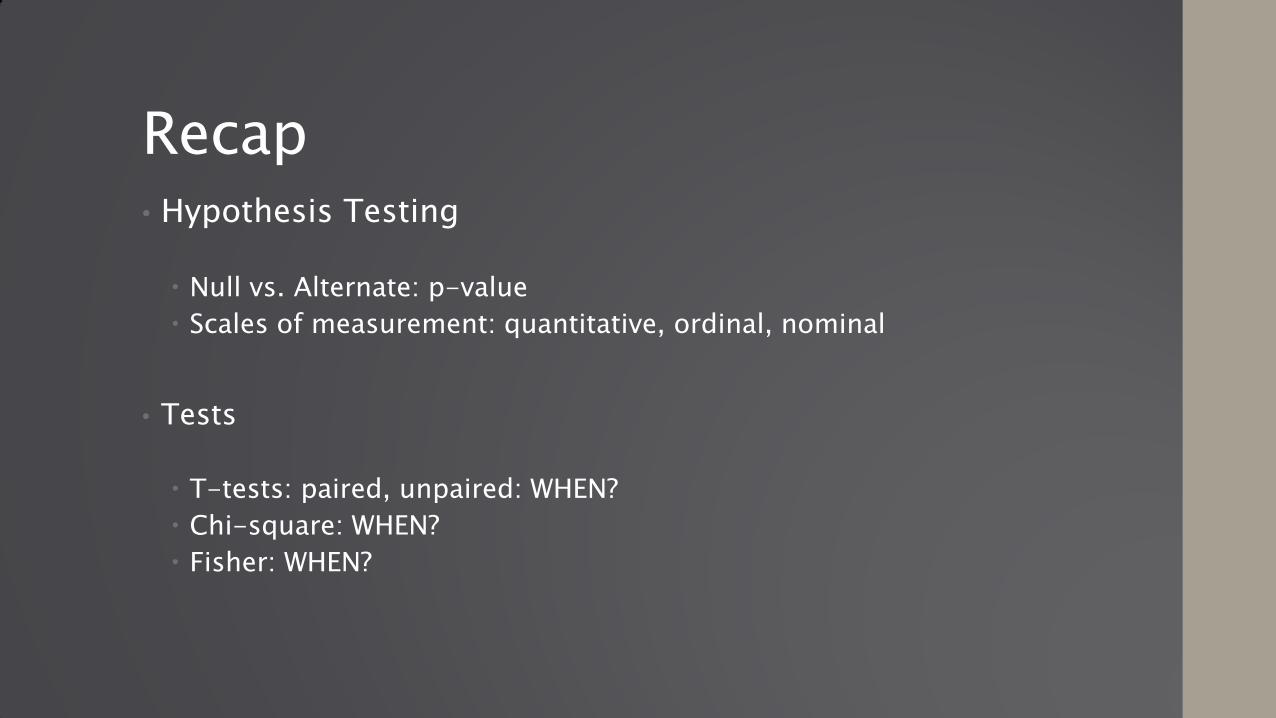
Recap • Hypothesis Testing

Null vs. Alternate: p-value

Scales of measurement: quantitative, ordinal, nominal

• Tests

T-tests: paired, unpaired: WHEN?

Chi-square: WHEN?

Fisher: WHEN?

Hypothesis Testing

• H0 : Null Hypothesis

The difference observed is due to a sampling error

• H1: Alternative Hypothesis

The difference observed is a “significant” difference,

due to the independent variable

Hypothesis Testing

• p-value: How likely is the sample obtained, if the null

hypothesis holds true.

• A threshold of significance = 0.05 (typically)

• Example: Does the time taken to complete a

transaction decrease when a design element is

modified?

Fisher’s Test

When: Data is nominal/categorical

small sample size (cell counts <10)

A/B Testing for 2 website versions (click-rate)

Compares: Means of two or more independent groups

Assumptions: Independent samples

Fisher’s Test in R

Do men and women differ in their preference for online surveys

and personal interviews?

f <- read.csv(“f.csv”)

fisher.test(f) : p-value = 1 : no significant difference

PI Online Surveys Total

Men 6 2 8

Women 8 4 12

Total 14 6 20

Rank Sum Tests

• Mann Whitney’s U Test

When: Dependent variable is ordinal AND/OR normality cannot

be assumed

Compares: Medians of two independent groups

Example 1: Do men and women rate a product’s functionality

differently?

Mann Whitney’s U Test

Do men and women rate a product’s functionality differently?

Likert Scale Ratings (1-5):

Calculation of Ranks

Men 2 4 4 1 3 3

Women 4 4 5 5 3 4

Men 2 (R2) 4 (R8) 4 (R7) 1 (R1) 3 (R3) 3 (R4)

Women 4 (R10) 4 (R9) 5 (R11) 5 (R12) 3 (R5) 4 (R6)

Mann Whitney’s U Test

Do men and women rate a product’s functionality differently?

Calculation of Ranks

Un-tied ranks (take averages of possible ranks):

Men 2 (R2) 4 (R8) 4 (R7) 1 (R1) 3 (R3) 3 (R4)

Women 4 (R10) 4 (R9) 5 (R11) 5 (R12) 3 (R5) 4 (R6)

Men 2 (R2) 4 (R8) 4 (R8) 1 (R1) 3 (R4) 3 (R4)

Women 4 (R8) 4 (R8) 5 (R11.5) 5 (R11.5) 3 (R4) 4 (R8)

Mann Whitney’s U Test

Un-tied ranks (take averages of possible ranks):

U1: Sum of Group 1 Ranks – n1 (n1+1)/2

U1 = 27 – (6 x 7)/2 = 6

U2: Sum of Group 2 Ranks – n2(n2+1)/2

U1 = 51 – (6 x 7)/2 = 30

Check that U1+U2 = n1n2

Lower U value tested for significance

Men 2 (R2) 4 (R8) 4 (R8) 1 (R1) 3 (R4) 3 (R4)

Women 4 (R8) 4 (R8) 5 (R11.5) 5 (R11.5) 3 (R4) 4 (R8)

Mann Whitney’s U Test in R • Men = c(2,4,4,1,3,3)

• Women = c(4,4,5,5,3,4)

• wilcox.test(Men, Women)

Mann Whitney’s U Test in R • library(coin)

• g = factor(c(rep("Men", length(Men)), rep("Women", length(Women))))

• v = c(Men, Women)

• wilcox_test(v ~ g, distribution="exact")

• Effect size (r) : Z/sqrt(total samples) : 2.0115/12 = 0.167

Mann Whitney Test

• How to report your results

• The medians of Men and Women were 3 and 4, respectively.

A Mann Whitney U test showed no significant effect of

gender on product ratings (U = 6, p > 0.05, Z = -2.011 , r

=0.167 )

• p-value > 0.05: Ho accepted

Mann Whitney U Test

Example 2: Do two search engines rate webpages differently?

Find out the U value!

Google 1 2 3 5 4

Bing 7 6 5 8 9

g = factor(c(rep("Google", length(Google)), rep("Bing", length(Bing))))

v = c(Google, Bing)

wilcox_test(v ~ g, distribution="exact")

W = 0.5, Z = 2.5143, p-value = 0.01587

Cheat Sheet: Which Test When

Group Type Quantitative Data

(Normality

assumed)

Ordinal Data or

Quantitative

(Normality not

assumed)

Nominal Data

Two unpaired groups Unpaired t test Mann-Whitney test Fisher's test

Two paired groups Paired t test Wilcoxon test McNemar's test

More than two

unmatched groups

ANOVA Kruskal-Wallis test Chi-square test

Resources for Statistics

• Statistics in HCI

http://yatani.jp/teaching/doku.php?id=hcistats:start

• Biostatistics Handbook

http://www.biostathandbook.com/index.html

• Statistics for Dummies

https://www.khanacademy.org/math/probability