Nonlinear FEM

5Critical Points

NFEM Ch 5 – Slide 1

Nonlinear FEM

Assumptions for this Chapter

=∂u

K = ∂r(u, λ)

r(u, λ)

∂u= ∂ �(u, λ)

∂�(u, λ)

∂u ∂u

System is conservative: total residual is the gradient of atotal potential energy function

Consequence: the tangent stiffness matrix (Hessian of Π)

is real symmetric

2

NFEM Ch 5 – Slide 2

Spectral Properties of Tangent Stiffness Matrix

Nonlinear FEM

K zi = κi zi , i = 1, 2, . . . N

Since K is real symmetric, it enjoys two important spectral properties:

. All eigenvalues of K are real

. K has a complete set of real eigenvectors, which can be orthonormalized so that

in which δ denotes the Kronecker delta

zTi z j = δij

ij

The algebraic eigenproblem for K has the form

NFEM Ch 5 – Slide 3

Regular Versus Critical

Nonlinear FEM

Regular point: K is nonsingularCritical point: K is singular (also called singular or nonregular points)

Useful criterion for small systems with small # of DOF:

The determinant of K vanishes at a critical point

NFEM Ch 5 – Slide 4

Why Are Critical Points Important?

Nonlinear FEM

Along a static equilibrium path of a conservative system,the transition from stability to instability (or vice-versa) always occurs at a critical point

Notes: (1) This does not mean that the transition will happen (2) Property does not extend to nonconservative systems

Consequence: in designing against instability, the analyst is primarily interested in locating critical points

NFEM Ch 5 – Slide 5

Critical Point Classification as per Number of Zero Eigenvalues (= Rank Deficiency)

Nonlinear FEM

Isolated critical point: K has one zero eigenvalue (= rank deficiency of K is one)

Multiple critical point: K has two or more zero eigenvalues (= rank deficiency of K is two or more)

We will focus on the isolated type for now, since multiplecritical points are more difficult to deal with

NFEM Ch 5 – Slide 6

Classification of Isolated Critical Points

Nonlinear FEM

Limit point: path continues with no branching, buttangent is normal to λ (control parameter) axis

Bifurcation point: two or more paths cross and there isno unique tangent

A limit point may be a maximum, minimum or inflexionpoint. If a maximum or minimum, its occurrence is alsocalled snap-through or snap-buckling by structural engineers

NFEM Ch 5 – Slide 7

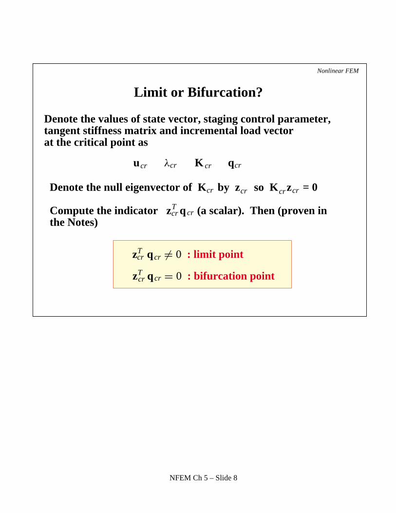
Limit or Bifurcation?

Nonlinear FEM

u λ K q

Denote the values of state vector, staging control parameter, tangent stiffness matrix and incremental load vector at the critical point as

Denote the null eigenvector of K by z so K z = 0

Compute the indicator z q (a scalar). Then (proven inthe Notes)

cr cr

cr

cr cr

cr

cr cr

cr cr

cr cr cr cr

zT

T

q �= 0 : limit point

zT q = 0 : bifurcation point

NFEM Ch 5 – Slide 8

Response Example (2 DOF,pictured in 2D control-state space)

Nonlinear FEM

Bifurcation beforelimit point

Limit point beforebifurcation

u

λ

B

L1

L2

1

λ L1

L2

B2

1B

u1

NFEM Ch 5 – Slide 9

Nonlinear FEM

Response Example (2 DOF,pictured in 3D control-state space)

Bifurcation beforelimit point

λ L1

L 2

B2

1B

u1u2

NFEM Ch 5 – Slide 10

A Simple Example (from Notes) Nonlinear FEM

r = u − 2 u + u − λ = 02 3

Find the critical points of the scalar residual equation

To be worked out on whiteboard

NFEM Ch 5 – Slide 11

The Circle Game Example Nonlinear FEM

r µ, λ = λ − µ λ2 + µ2 − 1 = 0

(Artificial, not associated with a real structure)

−1 −0.5 0 0.5 1

−1

−0.5

0

0.5

1

State parameter µ

Con

trol

par

amet

er λ

R

L1

B1

B2

T1

S2

S1

L2

T2

Total residual:

NFEM Ch 5 – Slide 12

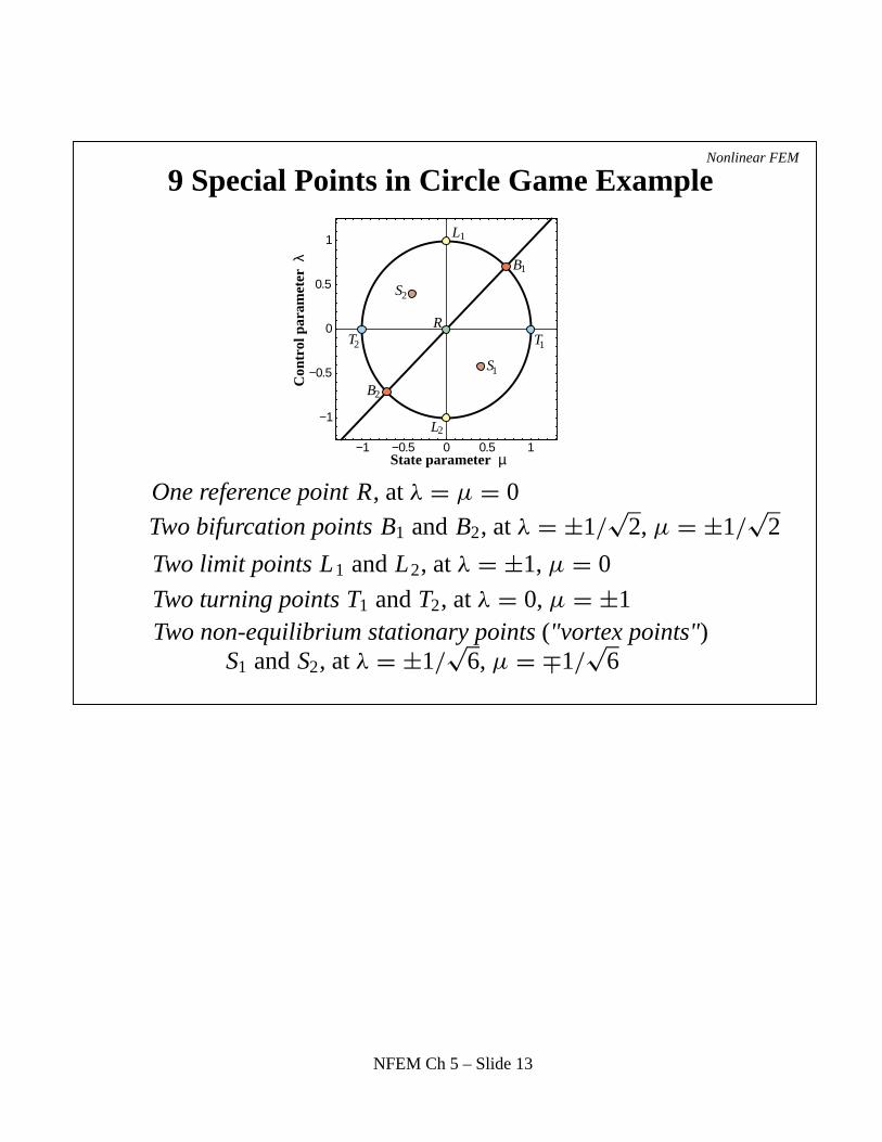
9 Special Points in Circle Game ExampleNonlinear FEM

One reference point R, at λ = µ = 0

Two bifurcation points B1 and B2, at λ = ±1/√

2, µ = ±1/√

2

Two limit points L1 and L2, at λ = ±1, µ = 0

Two turning points T1 and T2, at λ = 0, µ = ±1Two non-equilibrium stationary points ("vortex points")

S1 and S2, at λ = ±1/√

6, µ = ∓1/√

6

−1 −0.5 0 0.5 1

−1

−0.5

0

0.5

1

State parameter µ

Con

trol

par

amet

er λ

R

L1

B1

B2

T1

S2

S1

L2

T2

NFEM Ch 5 – Slide 13

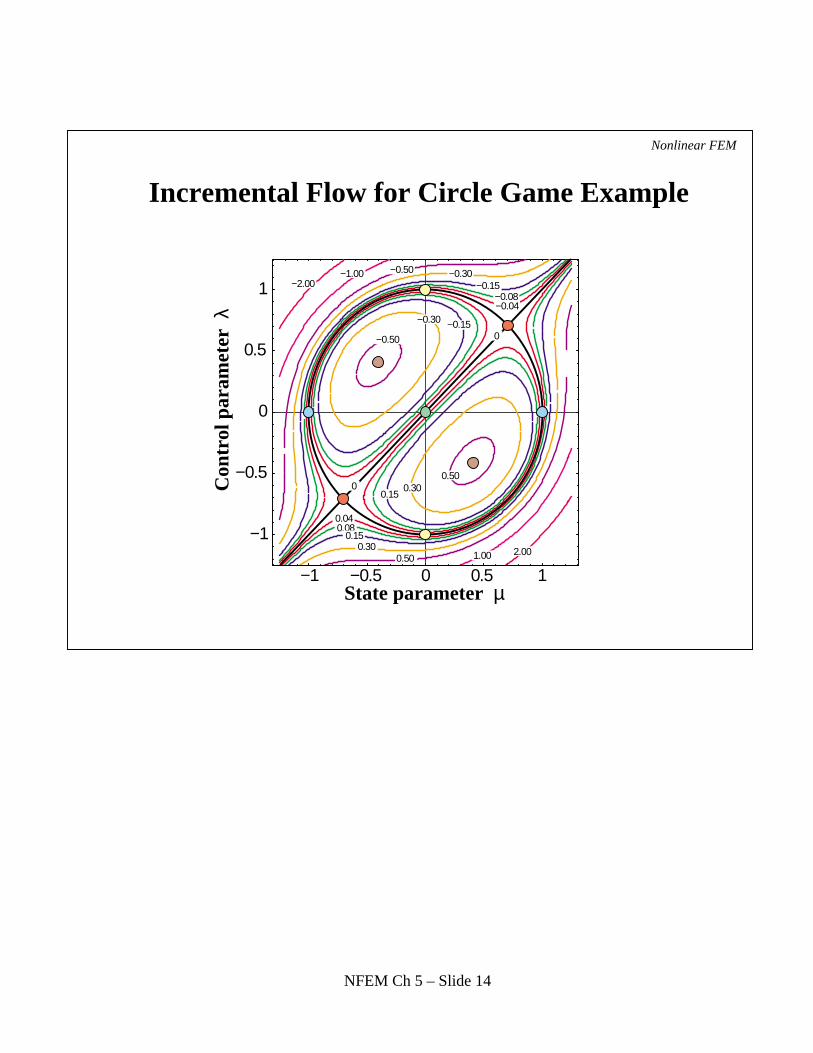
Incremental Flow for Circle Game Example

Nonlinear FEM

−1 −0.5 0 0.5 1

−1

−0.5

0

0.5

1

State parameter µ

Con

trol

par

amet

er λ

0.04

0

0

0.080.15

0.15

0.30

0.30

0.50

0.50

1.00 2.00

−0.04−0.08

−0.15

−0.15

−0.30

−0.30

−0.50

−0.50

−1.00−2.00

NFEM Ch 5 – Slide 14

Tangent Stiffness, Incremental Load, andIncremental Velocity for Circle Game Example

Nonlinear FEM

K = ∂r

∂µ= 1 − λ2 + 2λµ − 3µ2

q = − ∂r

∂λ= 1 − 3λ2 + 2λµ − µ2

v = q/K

For 1 DOF these matrix and vector quantities reduceto scalars:

NFEM Ch 5 – Slide 15

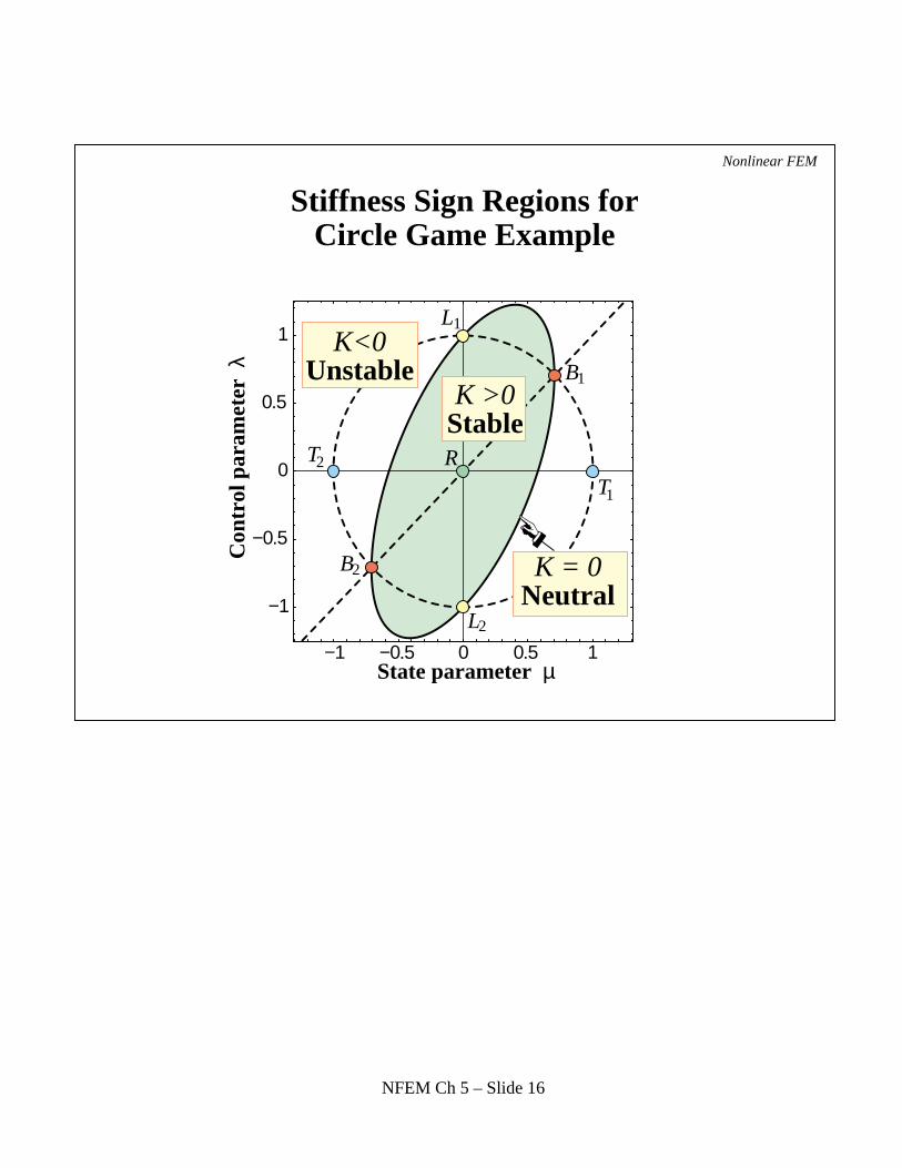
Stiffness Sign Regions for Circle Game Example

Nonlinear FEM

−1 −0.5 0 0.5 1

−1

−0.5

0

0.5

1

State parameter µ

Con

trol

par

amet

er λ

R

L1

B1

B2

T1

L2

T2

K >0Stable

K<0Unstable

K = 0Neutral

NFEM Ch 5 – Slide 16

Incremental Load Sign Regions for Circle Game Example

Nonlinear FEM

−1 −0.5 0 0.5 1

−1

−0.5

0

0.5

1

State parameter µ

Con

trol

par

amet

er λ

R

L1

B1

B2

T1

L2

T2

q = 0

q > 0

q< 0

NFEM Ch 5 – Slide 17

Incremental Velocity Sign Regions for Circle Game Example

Nonlinear FEM

−1 −0.5 0 0.5 1

−1

−0.5

0

0.5

1

State parameter µ

Con

trol

par

amet

er λ

R

L1

S1

S2

B1

B2

T1

L2

T2

K = 0

q=0 & v=0

v=q/K=0/0

NFEM Ch 5 – Slide 18

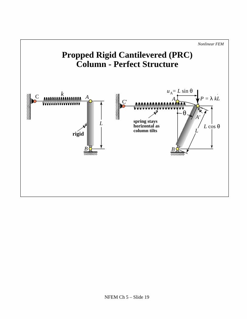
Propped Rigid Cantilevered (PRC)Column - Perfect Structure

Nonlinear FEM

����

A

B

��� k

A'

A

B

P = λ kL

u = L sin θA

������

rigid

L

����

θ

CC'

spring stayshorizontal ascolumn tilts L

L cos θ

NFEM Ch 5 – Slide 19

Perfect PRC Column: Response

Nonlinear FEM

Control versus state parameter response for perfect column

Tangent stiffness versus state parameter response for perfect column

B

State parameter µState parameter µ

Con

trol

par

amet

er λ

Stif

fnes

s co

effi

cien

t K

−1 −0.5 0 0.5 1

−0.75−0.5

−0.250

0.250.5

0.751

B

R T1T2−1 −0.5 0 0.5 1

0.2

0.4

0.6

0.8

1

1.2

1.4

Unstable Unstable

Stable

Unstable

λcr

NFEM Ch 5 – Slide 20

Propped Rigid Cantilevered (PRC)Column - Imperfect Structure

Nonlinear FEM

��B

��� k

A'AA

B

���

��

θ

CC'

εL

InitialImperfection

θ0θ0

A0A0

L

rigid

spring stayshorizontal ascolumn tilts

P = λ kLu = L sin θA

L cos θL

NFEM Ch 5 – Slide 21

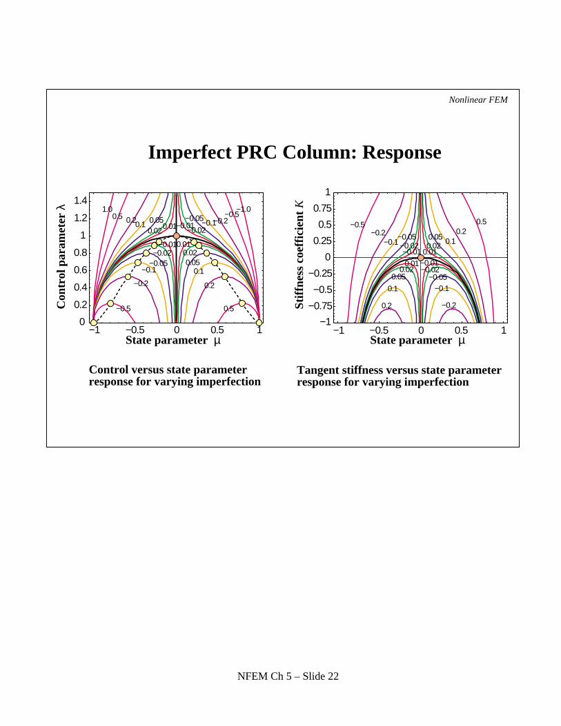
Control versus state parameter response for varying imperfection

Tangent stiffness versus state parameter response for varying imperfection

−1 −0.5 0 0.5 1

0.2

0.4

0.6

0.8

1

1.2

1.4

−1 −0.5 0 0.5 1

−0.75−0.5

−0.250

0.250.5

0.751

State parameter µState parameter µ

Con

trol

par

amet

er λ

Stif

fnes

s co

effi

cien

t K

0.01

0.01

−0.01

−0.01

0.02

0.02

0.05

0.05

0.1

0.1

0.2

0.2

0.5

0.51.0

−0.02

−0.02

−0.05

−0.05

−0.1

−0.1

−0.2

−0.2

−0.5

−0.5−1.0

0.010.01−0.01

−0.010.02

0.02

0.05

0.05

0.1

0.1

0.2

0.20.5

−0.02

−0.02

−0.05

−0.05−0.1

−0.1

−0.2

−0.2−0.5

0 −1

Imperfect PRC Column: Response

Nonlinear FEM

NFEM Ch 5 – Slide 22

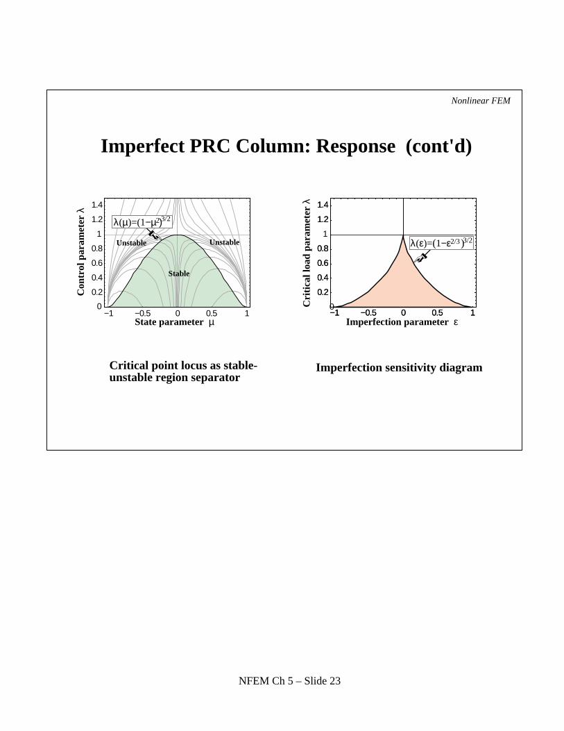
Imperfect PRC Column: Response (cont'd)

Critical point locus as stable-unstable region separator

Imperfection sensitivity diagram

−1 −0.5 00 0

0.5 1

0.2

0.4

0.6

0.8

1

1.2

1.4

State parameter µ Imperfection parameter ε

Con

trol

par

amet

er λ

Cri

tica

l loa

d pa

ram

eter

λ

Unstable Unstable

Stable

−1 −0.5 0 0.5 1

0.2

0.4

0.6

0.8

1.2

1.4

−1 −0.5 0 0.5 1

0.2

0.4

0.6

0.8

1

1.2

1.4

λ(µ)=(1−µ )2 3/2

λ(ε)=(1−ε )3/2 2/3

Nonlinear FEM

NFEM Ch 5 – Slide 23