Critical Parameter Values and Reconstruction Propertiesof Discrete

Fundamenta Informaticae 125 (2013) 285–312 285DOI 10.3233/FI-2013-865IOS Press

Critical Parameter Values and Reconstruction Properties ofDiscrete Tomography: Application to Experimental Fluid Dynamics

Stefania Petra∗†

Image and Pattern Analysis Group, University of Heidelberg

Speyerer Str. 6, 69115 Heidelberg, Germany

[email protected]

Christoph SchnorrImage and Pattern Analysis Group, University of Heidelberg

[email protected]

Andreas SchroderInstitute of Aerodynamics and Flow Technology, German Aerospace Center

Bunsenstr. 10, 37073 Gottingen, Germany

[email protected]

Abstract. We analyze representative ill-posed scenarios of tomographic PIV (particle image ve-locimetry) with a focus on conditions for unique volume reconstruction. Based on sparse randomseedings of a region of interest with small particles, the corresponding systems of linear projectionequations are probabilistically analyzed in order to determine: (i) the ability of unique reconstruc-tion in terms of the imaging geometry and the critical sparsity parameter, and (ii) sharpness of thetransition to non-unique reconstruction with ghost particles when choosing the sparsity parameterimproperly. The sparsity parameter directly relates to the seeding density used for PIV in experi-mental fluids dynamics that is chosen empirically to date. Our results provide a basic mathematicalcharacterization of the PIV volume reconstruction problem that is an essential prerequisite for anyalgorithm used to actually compute the reconstruction. Moreover, we connect the sparse volumefunction reconstruction problem from few tomographic projections to major developments in com-pressed sensing.

Keywords: compressed sensing, underdetermined nonnegative linear systems, sparsity, large devi-ation, tail bound, limited angle tomography, TomoPIV

∗Support by the German Research Foundation (DFG) is gratefully acknowledged, grant SCHN457/11.†Address for correspondence: Image and Pattern Anal. Gr., Univ. of Heidelberg, Speyerer Str. 6, 69115 Heidelberg, Germany

286 S. Petra et al. / Weak Recovery Thresholds for TomoPIV

1. Introduction

1.1. Overview, Motivation

In our previous recent work [13] we pointed out the close connection between a 3D tomographic mea-surement technique that is driving current research work in experimental fluid dynamics, and the abstractproblem class concerned with the reconstruction of sparse solutions of underdetermined systems in thefield of compressed sensing. This connection is relevant because in the former field knowing how toavoid spurious reconstructions is crucial for applications. Yet, a theoretical underpinning of current prac-tice is lacking so far. On the other hand, research in compressed sensing addresses the problem to deviseperformance guarantees for ill-posed reconstruction problems under suitable mathematical assumptions.

In [13] we mainly worked out the gap between practice in the former field and theoretical results inthe latter, and additionally provided numerical evidence that the actual gap might be considerably smaller,which calls for appropriately modifying the mathematical requirements. In fact, the reconstruction of arandom sparse solution will be based on a reduced linear system with (on average) better reconstructionproperties. In the present paper we elaborate the latter point and report results of a thorough correspond-ing numerical study.

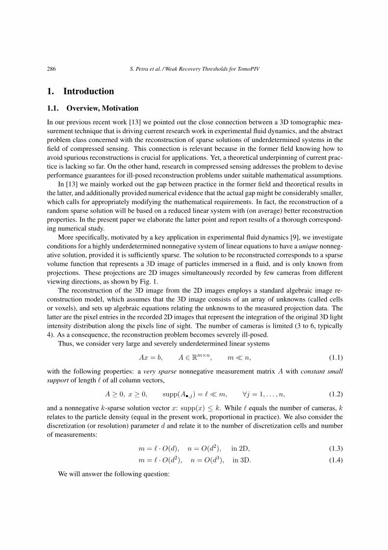
More specifically, motivated by a key application in experimental fluid dynamics [9], we investigateconditions for a highly underdetermined nonnegative system of linear equations to have a unique nonneg-ative solution, provided it is sufficiently sparse. The solution to be reconstructed corresponds to a sparsevolume function that represents a 3D image of particles immersed in a fluid, and is only known fromprojections. These projections are 2D images simultaneously recorded by few cameras from differentviewing directions, as shown by Fig. 1.

The reconstruction of the 3D image from the 2D images employs a standard algebraic image re-construction model, which assumes that the 3D image consists of an array of unknowns (called cellsor voxels), and sets up algebraic equations relating the unknowns to the measured projection data. Thelatter are the pixel entries in the recorded 2D images that represent the integration of the original 3D lightintensity distribution along the pixels line of sight. The number of cameras is limited (3 to 6, typically4). As a consequence, the reconstruction problem becomes severely ill-posed.

Thus, we consider very large and severely underdetermined linear systems

Ax = b, A ∈ Rm×n, m n, (1.1)

with the following properties: a very sparse nonnegative measurement matrix A with constant smallsupport of length of all column vectors,

A ≥ 0, x ≥ 0, supp(A•,j) = m, ∀j = 1, . . . , n, (1.2)

and a nonnegative k-sparse solution vector x: supp(x) ≤ k. While equals the number of cameras, krelates to the particle density (equal in the present work, proportional in practice). We also consider thediscretization (or resolution) parameter d and relate it to the number of discretization cells and numberof measurements:

m = ·O(d), n = O(d2), in 2D, (1.3)

m = ·O(d2), n = O(d3), in 3D. (1.4)

We will answer the following question:

S. Petra et al. / Weak Recovery Thresholds for TomoPIV 287

Figure 1. Typical camera arrangements: in circular configuration (right) or all in line (left).

What is the maximal number of particles, depending on the image resolution parameter d,that can be reconstructed uniquely?

Formally, we want to relate the exact recovery of x from it’s noiseless measurements b to the sparsity k

and to the dimensions of m,n of the projection matrix A. Moreover, we investigate critical values of thesparsity parameter k such that most k-sparse nonnegative vectors x are the unique nonnegative solutionof (1.1) for a given b with high probability.

Our results provide an answer to both the question above and to the problem of devising suitablerelaxations of the mathematical requirements as discussed in the beginning of this section. Moreover,our assumptions on the sensor matrix A conform to the imaging set-ups used in practice. Altogether, thiscloses the gap worked out in [13].

1.2. Related Work: Compressed Sensing

Research on compressed sensing [5, 3] focuses on properties of underdetermined linear systems thatguarantee exact recovery of sparse or compressible signals x from measurements b. Donoho and Tanner[7, 8] have computed sharp reconstruction thresholds for random measurement matrices such that for agiven signal length n and numbers of measurements m, the maximal sparsity value k which guaranteesperfect reconstruction can be determined explicitly. The authors derived their results by connecting it toa problem from geometric probability that n points in general position in Rm can be linearly separated[18]. This holds with probability Pr(n,m) = 1 for n/m ≤ 1, and with Pr(n,m) → 1 if m → ∞ and1 ≤ n/m < 2, where

Pr(n,m) =1

2n−1

m−1

i=0

n− 1

i

. (1.5)

The authors show in [7, Thm. 1.10] that the probability of uniqueness of a k-sparse nonnegative vectorequals Pr(n − m,n − k), provided A satisfies certain conditions which do not hold in our consideredapplication. Likewise, by exploiting again Wendel’s theorem Mangasarian and Recht showed [12] thata binary solution is most likely unique if m/n > 1/2, provided that A comes from a centrosymmetricdistribution. Unfortunately, the underlying distribution A lacks symmetry with respect to the origin.However, we recently showed in [14] that for a three camera scenario there are thresholds on sparsity(i.e. density of the particles), below which exact recovery will succeed and above which it fails with high


probability. These explicit thresholds depend on the number of measurements (recording pixels in thecamera arrays). The current work investigates further geometries and focuses on an average case analysisof conditions under which uniqueness of x can be expected with high probability. A corresponding tailbound implies a weak threshold effect and a criterion for adequately choosing the (maximal) value of thesparsity parameter k.

1.3. Connection to Tomographic PIV and Discrete Tomography

The measurement technique Particle Image Velocimetry (PIV) is concerned with the inference of theinstantaneous motion of fluids from image measurements. In this context, Tomographic PIV (TomoPIV)[9] addressed the problem to reconstruct the time-varying 3D image function in a preprocessing step. Akey property of this measurement technique is that at the subsequent processing stage motion estimationtechniques can invoke physical prior knowledge (e.g. incompressibility) due to working directly in 3Dspace. We refer to [15, 16] for further details.

A crucial requirement in this connection concerns the accuracy of the reconstructed 3D image func-tion as input data for motion estimation. This critically depends on the particle density or – mathemati-cally speaking – on the sparsity of the solution. Engineers aim at using high particle densities (less sparsesolutions) to enable motion estimates with high spatial resolution at the subsequent processing stage. Us-ing too high densities will inevitably lead to spurious reconstructions, and in turn to erroneous motionestimates. On the other hand, conservatively chosen low particle densities will merely lead to motion es-timates at some coarse spatial resolution and hence compromise TomoPIV as an advanced measurementtechnique.

The present paper studies mathematically substantiated choices of maximal particle densities thatprovide accurate reconstructions.

Finally, we point out the connection of our work to discrete tomography [10]. In this research areadiscrete representations are used both for indexing the underlying domain and for the range of values ofthe function to be reconstructed from measurements. By contrast, in our setting a continuous boundedspatial domain is discretized by means of expanding the function of interest with compactly supportedbasis functions (e.g. just indicator functions of voxels), and rather than focusing on discrete-valued func-tions we focus on the discrete range of the number of non-vanishing coefficients. In our opinion thisdifference is not a significant one because computational approaches to large-scale discrete tomogra-phy typically involve some relaxation, for instance by replacing an integer constraint xi ∈ 0, 1 byxi ∈ [0, 1]. This blurs the boundary the term ”discrete” seems to suggest.

1.4. Contribution and Organization

Our contribution concerns the probabilistic analysis of the dimension of reduced systems (Definition 2.3)depending on the sparsity parameter k, in terms of its expected value together with a deviation bound.Sharp concentration in terms of the latter bound assures that uniqueness holds with high probability, thatis informally speaking in most applications.

Such an analysis was recently introduced in [14] for the specific academical scenario considered inour previous work [13]. The present paper extends this analysis to a broader range of scenarios thatrepresent realistic imaging set-ups. Major examples include the set-up depicted by Figure 2, that covers


2D scenarios, which can be easily extended to 3D scenarios by enhancing both camera and volume byone dimension, and a “full” 3D set-up with 4 cameras illustrated by Fig. 3.

Section 2 establishes the connection between realistic sensing matrices used in TomoPIV and recentwork on sparse expander graphs in the field of compressed sensing. This enables to formulate criteriafor the unique reconstruction of sparse solutions in terms of the dimension of the corresponding reducedsystem. Moreover, our theoretical analysis suggests that a similar procedure can be applied to differentgeometries varying the volume size, number of discretization cells and number of projections.

The expected dimension of various imaging set-ups are estimated in Sections 3 and 4. These esti-mates accurately agree with results from a series of numerical experiments that illustrate in Section 5 theseparation of non-recovery and recovery by phase transitions.

We conclude and indicate directions for further research in Section 6.

1.5. Notation

|X| denotes the cardinality of a finite set X and [n] = 1, 2, . . . , n for n ∈ N. We will denote byx0 = |i : xi = 0| and Rn

k = x ∈ Rn : x0 ≤ k the set of k-sparse vectors. The correspondingsets of non-negative vectors are denoted by Rn

+ and Rnk,+ respectively. The support of a vector x ∈ Rn,

supp(x) ⊆ [n], is the set of indices of non-vanishing components of x.For a finite set S, the set N (S) denotes the union of all neighbors of elements of S where the

corresponding relation (graph) will be clear from the context.1 = (1, . . . , 1) denotes the one-vector of appropriate dimension.A•,i denotes the i-th column vector of a matrix A. For given index sets I and J , matrix AIJ denotes

the submatrix of A with rows and columns indexed by I and J respectively. Ic, Jc denote the respectivecomplement sets. Similarly, bI denotes a subvector of b.

E[·] denotes the expectation operation applied to a random variable and Pr(A) the probability toobserve an event A.

2. Graph Related Properties of Tomographic Projection Matrices

Recent trends in compressed sensing [2, 19] tend to replace random dense matrices by adjacency matricesof ”high quality” expander graphs. Explicit constructions of such expanders exist, but are quite involved.However, random m × n binary matrices with nonreplicative columns that have n entries equal to1, perform numerically quite well, even if is small, as shown in [2]. In [11, 13] it is shown thatperturbing the elements of adjacency matrices of expander graphs with low expansion can also improveperformance.

2.1. Preliminaries

For simplicity, we will confine ourselves to situations where the intersection lengths of projection rayscorresponding to each camera with each discretization cell are all equal. Thus, we assume that the entriesof A are binary. It will be useful to denote the set of cells by C = [n] and the set of rays by R = [m].


The incidence relation between cells and rays is then given by

(A)ij =

1, if j-th ray intersects i-th cell,0, otherwise,

(2.1)

for all i ∈ R, j ∈ C. Thus, cells and rays correspond to columns and rows of A.This gives the equivalent representation in terms of a bipartite graph G = (C,R;E) with left and

right vertices C and R, and edges (c, r) ∈ E iff (A)rc = 1. G has constant left-degree equal to thenumber of projecting directions.

For any non-negative measurement matrix A and the corresponding graph, the set

N (S) = i ∈ [m] : Aij > 0, j ∈ S

contains all neighbors of S. The same notation applies to neighbors of subsets S ⊂ R of right nodes.Further, we will call any non-negative matrix adjacency matrix, based on the incidence relation of itsnon-zero entries.

If A is the non-negative adjacency matrix of a bipartite graph with constant left degree , theperturbed matrix A is computed by uniformly perturbing the non-zero entries Aij > 0 to obtainAij ∈ [Aij − ε, Aij + ε], and by normalizing subsequently all column vectors of A. In practice, suchperturbation can be implemented by discretizing the image by radial basis functions of unequal size orby choosing their locations on an irregular grid.

The following class of graphs plays a key role in the present context and in the field of compressedsensing in general.

Definition 2.1. A (ν, δ)-unbalanced expander is a bipartite simple graph G = (L,R;E) with constantleft-degree such that for any X ⊂ L with |X| ≤ ν, the set of neighbors N (X) ⊂ R of X has at leastsize |N (X)| ≥ δ|X|.

Recovery of a k-sparse nonnegative solution via an (ν, δ)-unbalanced expander was derived in [17].It employs the smallest expansion constant δ with respect to other similar results in the literature.

Theorem 2.2. Let A be the adjacency matrix of a (ν, δ)-unbalanced expander and 1 ≥ δ >

√5−12 . Then

for any k-sparse vector x∗ with k ≤ν

(1+δ) , the solution set x : Ax = Ax∗, x ≥ 0 is a singleton.

Now let A denote the tomographic projection matrix, and consider a subset X ⊂ C of |X| = k

columns and a corresponding k-sparse vector x supported on X . Then b = Ax has support N (X), andwe may remove the subset of N (X)c = (N (X))c rows from the linear system Ax = b corresponding tobr = 0, ∀r ∈ R. Moreover, based on the observation N (X), we know that

X ⊆ N (N (X)) and N (N (X)c) ∩X = ∅. (2.2)

We continue by formalizing the system reduction just described.

Definition 2.3. The reduced system corresponding to a given non-negative vector b,

Aredx = bred, Ared ∈ Rmred×nred+ , (2.3)


results from A, b by choosing the subsets of rows and columns

Rb := supp(b), Cb := N (Rb) \ N (Rcb) (2.4)

withmred := |Rb|, nred := |Cb|. (2.5)

Note that for a vector x and the bipartite graph induced by the measurement matrix A, we have thecorrespondence (cf. (2.2))

X = supp(x), Rb = N (X), Cb = N (N (X)) \ N (N (X)c).

We further defineS+ := x : Ax = b, x ≥ 0 (2.6)

andS+red := x : ARbCbx = bRb , x ≥ 0 . (2.7)

The following proposition asserts that solving the reduced system (2.3) will always recover the supportof the solution to the original system Ax = b

Proposition 2.4. [14, Prop. 5.1] Let A ∈ Rm×n and b ∈ Rm have nonnegative entries only, and let S+

and S+red be defined by (2.6) and (2.7) respectively. Then

S+ = x ∈ Rn : x(Cb)c = 0 and xCb ∈ S

+red. (2.8)

Consequently, we can restrict the linear system Ax = b to the subset of columns N (N (X)) \N (N (X)c) ⊂ C, and only consider properties of this reduced systems.

2.2. Guaranteed Uniqueness

Uniqueness of x ∈ Rnδk,+ is guaranteed if all k or less-sparse supported on supp(x) induce overdeter-

mined reduced systems with mred/nred > δ ≥

√5−12 .

Proposition 2.5. [14, Th. 3.4] Let A be the adjacency matrix of a bipartite graph such that for all randomsubsets X ⊂ C of |X| ≤ k left nodes, the set of neighbors N (X) of X satisfies

|N (X)| ≥ δ|N (N (X)) \ N (N (X)c)| with δ >

√5− 1

2. (2.9)

Then, for any δk-sparse nonnegative vector x∗, the solution set x : Ax = Ax∗, x ≥ 0 is a singleton.

For perturbed matrices uniqueness is guaranteed for square reduced systems, and thus less sparse solu-tions.

Proposition 2.6. [14, Th. 3.4] Let A be the adjacency matrix of a bipartite graph such that for all subsetsX ⊂ C of |X| ≤ k left nodes, the set of neighbors N (X) of X satisfies

|N (X)| ≥ δ|N (N (X)) \ N (N (X)c)| with δ >1

. (2.10)

Then, for any k-sparse vector x∗, there exists a perturbation A of A such that the solution set x : Ax =Ax∗, x ≥ 0 is a singleton.


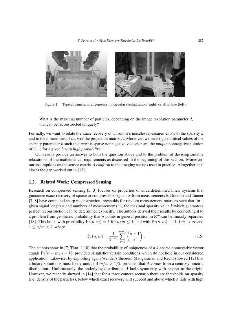
Figure 2. Sketch of a 3-cameras setup in 2D. Left: The hexagonal area discretized in 3· d2+14 equally sized cells is

projected on three 1D cameras. The resulting projection matrix A ∈ 0, 1m×n is underdetermined, with m = 3d

and n = 3· d2+14 , where d−1

2 +1 is the number of cells on each hexagon edge. Middle: This geometry can be easilyextended to 3D by enhancing both cameras and volume by one dimension, thus representing scenarios of practicalrelevance when cameras are aligned on a line. Right: When considering a square area along with three projectiondirections (two orthogonal, one diagonal) one obtains a projection matrix with analogous reconstruction properties.The projection matrix equals up to scaling the previous projection matrix corresponding to the hexagonal area, ifwe remove the 2 · d2−1

8 cells in the marked corners along with incident rays.

Recovery via perturbed underdetermined reduced systems is possible and our numerical results fromSection 5 suggest the following.

Conjecture 2.7. Let A be the adjacency matrix of a bipartite graph such that for all subsets X ⊂ C of|X| ≤ k left nodes, the set of neighbors N (X) of X satisfies

|N (X)| ≥1 + δ

|N (N (X)) \ N (N (X)c)| with δ >

√5− 1

2. (2.11)

Then, for any k -sparse vector x∗, there exists a perturbation A of A such that the solution set x : Ax =

Ax∗, x ≥ 0 is a singleton.

The consequences of Propositions 2.5, 2.6 and Conjecture 2.7 are investigated in the following sec-tions 3.2 and 4.2 by working out critical values of the sparsity parameter k for which the respectiveconditions are satisfied with high probability.

3. 3 Cameras - Left Degree equals 3

In this section, we analyze the imaging set-up depicted in Figure 2, left panel, which also representstypical 3D scenarios encountered in practice, as shown in Figure 2, center panel.


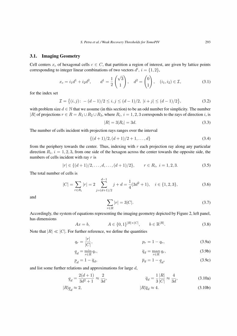
3.1. Imaging Geometry

Cell centers xc of hexagonal cells c ∈ C, that partition a region of interest, are given by lattice pointscorresponding to integer linear combinations of two vectors di, i = 1, 2,

xc = i1d1 + i2d

2, d

1 =1

2

√3

1

, d

2 =

0

1

, (i1, i2) ∈ I, (3.1)

for the index set

I =(i, j) : − (d− 1)/2 ≤ i, j ≤ (d− 1)/2, |i+ j| ≤ (d− 1)/2

, (3.2)

with problem size d ∈ N that we assume (in this section) to be an odd number for simplicity. The number|R| of projections r ∈ R = R1 ∪R2 ∪R3, where Ri, i = 1, 2, 3 corresponds to the rays of direction i, is

|R| = 3|Ri| = 3d. (3.3)

The number of cells incident with projection rays ranges over the interval

(d+ 1)/2, (d+ 1)/2 + 1, . . . , d (3.4)

from the periphery towards the center. Thus, indexing with r each projection ray along any particulardirection Ri, i = 1, 2, 3, from one side of the hexagon across the center towards the opposite side, thenumbers of cells incident with ray r is

|r| ∈ (d+ 1)/2, . . . , d, . . . , (d+ 1)/2, r ∈ Ri, i = 1, 2, 3. (3.5)

The total number of cells is

|C| =

r∈Ri

|r| = 2d−1

j=(d+1)/2

j + d =1

4(3d2 + 1), i ∈ 1, 2, 3, (3.6)

and

r∈R|r| = 3|C|. (3.7)

Accordingly, the system of equations representing the imaging geometry depicted by Figure 2, left panel,has dimensions

Ax = b, A ∈ 0, 1|R|×|C|, b ∈ R|R|

. (3.8)

Note that |R| |C|. For further reference, we define the quantities

qr =|r|

|C|, pr = 1− qr, (3.9a)

qd= min

r∈Rqr, qd = max

r∈Rqr, (3.9b)

pd= 1− qd, pd = 1− q

d, (3.9c)

and list some further relations and approximations for large d,

qd=

2(d+ 1)

3d2 + 1≈

2

3d, qd =

1

3

|R|

|C|≈

4

3d, (3.10a)

|R|qd≈ 2, |R|qd ≈ 4. (3.10b)


3.2. Dimensions of Reduced Systems

We estimate the expected dimensions (2.5) of the reduced system (2.3) based on uniformly selecting k

cells at random locations.To each projection ray r ∈ R, we associate a binary random variable Xr taking the value Xr = 1

if not any of the k cells is incident with ray r, and Xr = 0 otherwise. We call the event Xr = 1zero-measurement.

We are interested in the random variable

X =

r∈RXr (3.11)

that determines the number of projection rays not incident with any of the k cells, that is the number ofzero measurements. We set

N0R := E[X], NR := |R|−N

0R. (3.12)

Hence, NR is the expected size of the support mred = | supp(b)| of the measurement vector b.

Remark 3.1. Note that random variables Xr are not independent because different projection rays mayintersect. This dependency does not affect the expected value of X , but it does affect the deviation ofobserved values of X from its expected value – cf. Section 3.3.

Remark 3.2. We do not assume in the derivation below that k different cells are selected. In fact, asingle cell may be occupied by more than a single particle in practice, because real particles are verysmall relative to the discretization cells c. The imaging optics enlarges the appearance of particles, andthe action of physical projection rays is adequately represented by linear superposition.

Definition 3.3. (Sparsity Parameter)We refer to the number k introduced above as sparsity parameter. Thus, highly sparse scenarios corre-spond to low values k.

Lemma 3.4. The expected number N0R of zero measurements is

N0R = N

0R(k) = E[X] =

r∈Rpkr . (3.13)

Proof:For k = 1, Xr has a Bernoulli distribution with

E[Xr] = Pr[Xr = 1] = 1−|r|

|C|= 1− qr = pr. (3.14)

For k independent trials, we have (cf. Remark 3.2)

E[Xr] = Pr[Xr = 1] = pkr . (3.15)

By the linearity of expectations and (3.15), we obtain (3.13),

N0R = E[X] =

r∈RE[Xr] =

r∈Rpkr . (3.16)


We discuss few specific scenarios depending on the sparsity parameter k.

No particles For k = 0, we obviously have

N0R =

r∈R1 = |R|.

High sparsity By (3.10), we have qd≤ qr ≤ qd, hence qr = O(d−1). Thus, for large problem sizes d

and small values of k,

N0R ≈

r∈R

k

0

1kq0r −

k

1

1k−1

q1r

=

r∈R(1− kqr).

By (3.7),

r∈R qr = 3, henceN

0R ≈ |R|− 3k. (3.17)

This approximation says that for sufficiently small values of k each randomly selected cell can beexpected to create 3 independent measurements, which just reflects the fact that each cell is metby three projection rays.

Less high sparsity For increasing values of k higher-order terms cannot longer be ignored, due to theincreasing number of projection rays meeting several particles. Taking the second-order term intoaccount, we obtain in an analogous way

N0R ≈

r∈R(1− kqr +

k(k − 1)

2q2r )

≤

r∈R(1− kqr +

k(k − 1)

2qrqd) = |R|− 3k +

3

2k(k − 1)qd,

(3.18)

which is a fairly tight upper bound for values of k and N that are relevant to applications.

We consider next the expected number of cells nred = |Cb| of cells supporting the set Rb accordingto (2.4). We denote this expected number by

NC := E[|Cb|], N0C := |C|−NC , (3.19)

and by N0C the expected size of the complement.

Let R = R1∪R2∪R3 denote the partition of all projection rays by the three directions. For each cellc, there are three unique rays ri(c) ∈ Ri, i = 1, 2, 3, incident with c. Furthermore, for i = j and someray ri ∈ Ri, let Rj(ri) denote the set of rays that intersect with ri. As before, |r| denotes the number ofcells covered by projection ray r ∈ R.


Proposition 3.5. For a given sparsity parameter k, the expected number of cells that can be recognizedas empty based on the observations of random variables Xrr∈R is

N0C = N

0C(k) = 3N1

C − 3N2C +N

3C , (3.20a)

N1C =

r∈Ri

|r|

1−

|r|

|C|

k

, for any i ∈ 1, 2, 3, (3.20b)

N2C =

ri∈Ri

rj∈Rj(ri)

1−

|ri|+ |rj |− 1

|C|

k

, for any i, j ∈ 1, 2, 3, i = j, (3.20c)

N3C =

c∈C

1−

3i=1 |ri(c)|− 2

|C|

k

. (3.20d)

Proof:Each cell intersects with three projection rays ri(c), i = 1, 2, 3. Hence, given the rays corresponding tozero measurements, each cell that can be recognized as empty if either one, two or three rays from theset ri(c)i=1,2,3 belong to this set.

We therefore determine separately the expected number of removable cells (i) due to individual rayscorresponding to zero measurements, (ii) due to all pairs of rays that intersect and correspond to zeromeasurements, and (iii) due to all triples of rays that intersect and correspond to zero measurements. Theestimate (3.20a) corresponding to the union of these events results from the inclusion-exclusion principlethat combines these numbers so as to avoid overcounting.

Consider each projection ray r ∈ Ri for any fixed direction i = 1, 2, 3. Because these rays do notintersect, the expected number of cells that can be removed based on the observation Xrr∈R, is

N1C = E

r∈Ri

Xr|r|

=

r∈Ri

pkr |r| (3.21)

by the linearity of expectations and (3.15). Due to the symmetry of the setup, this number is the samefor each direction i = 1, 2, 3. Hence we multiply N1

C by 3 in (3.20a).Consider next pairs of directions i, j ∈ 1, 2, 3, i = j. For i fixed, the expected number of empty

cells based on a zero measurement corresponding to some ray ri ∈ Ri and all rays rj ∈ Rj(ri) inter-secting with ri, is

N2C = E

ri∈Ri

rj∈Rj(ri)

XriXrj

. (3.22)

The linearity of expectations and E[XriXrj ] = Pr(Xri = 1) ∧ (Xrj = 1)

gives (3.20c). Due to

symmetry, we have to multiply N2C by 3 in (3.20a).

Finally, the expected number of empty cells that correspond to observed zero measurements alongall three projection directions is

N3C = E

c∈C

3

i=1

Xri(c)

, (3.23)

which equals (3.20d).


An immediate consequence of Lemma 3.4 and Prop. 3.5 is

Corollary 3.6. For a given value of the sparsity parameter k, the expected dimensions of the reducedsystem (2.3) are

mred = NR −N0R, nred = NC −N

0C , (3.24)

with N0R, N

0C given by (3.13) and (3.20).

3.3. A Tail Bound

We are interested in how sharply the random number X of zero measurements peaks around its expectedvalue N0

R = E[X] given by (3.13).Because the random variables Xr, r ∈ R, are not independent, due to the intersection of projection

rays, we apply the following classical inequality for bounding the deviation of a random variable fromits expected value based on martingales, that is on sequences of random variables (Yi) defined on a finiteprobability space (Ω,F , µ) satisfying

E[Yi+1|Fi] = Xi, for all i ≥ 1, (3.25)

where Fi denotes an increasing sequence of σ-fields in F with Yi being Fi-measurable.

Theorem 3.7. (Azuma’s Inequality [1, 4])Let (Yi)i=0,1,2,... be a martingale such that for each i,

|Yi − Yi−1| ≤ ci. (3.26)

Then, for all j ≥ 0 and any δ > 0,

Pr|Yj − Y0| ≥ δ

≤ 2 exp

−

δ2

2j

i=1 c2i

. (3.27)

Let Fi ⊂ 2R, i = 0, 1, 2, . . . , denote the σ-field generated by the collection of subsets of R that cor-respond to all possible events after having observed i randomly selected cells. We set F0 = ∅, R.Observing cell i + 1 just further partitions the current state based on the previously observed i cellsby possibly removing some ray (or rays) from the set of zero measurements. Thus, we have a nestedsequence (filtration) F0 ⊆ F1 ⊆ · · · ⊆ Fk of the set 2R of all subsets of R.

Based on this, for a fixed value of the sparsity parameter k, we define the sequence of randomvariables

Yi = E[X|Fi], i = 0, 1, . . . , k, (3.28)

where Yi, i = 0, 1, . . . , k−1, are the random variables specifying the expected number of zero measure-ments after having observed k randomly selected cells, conditioned on the subset of events Fi determinedby the observation of i randomly selected cells. Consequently, Y0 = E[X] = N0

R due to the absenceof any information, and Yk = X is just the observed number of zero measurements. The sequence(Yi)i=0,...,k is a martingale by construction satisfying E[Yi+1|Fi] = Yi, that is condition (3.25).


Proposition 3.8. Let N0R = E[X] be the expected number of zero measurements for a given sparsity

parameter k, given by (3.13). Then, for any δ > 0,

Pr|X −N

0R| ≥ δ

≤ 2 exp

−

1− p2d

18(1− p2kd )δ2

. (3.29)

Proof:Let R0

i−1 ⊂ R denote the subset of rays with zero measurements after the random selection of i− 1 < k

cells. For the remaining k−(i−1) trials, the probability that not any cell incident with some ray r ∈ R0i−1

will be selected ispk−(i−1)r = E[Xr|Fi−1], (3.30)

with pr given by (3.14). Consequently, by the linearity of expectations, the expectation Yi−1 of zeromeasurements, given the number |R0

i−1| of zero measurements after the selection of i− 1 cells, is

Yi−1 = E[X|Fi−1] =

r∈R0i−1

pk−(i−1)r . (3.31)

Now suppose we observe the random selection of the i-th cell. We distinguish two possible cases.

1. Cell i is not incident with any ray r ∈ R0i−1. Then the number of zero measurements remains the

same, andYi =

r∈R0i−1

pk−ir . (3.32)

Furthermore,

Yi − Yi−1 =

r∈R0i−1

pk−ir − p

k−(i−1)r

=

r∈R0i−1

pk−ir (1− pr)

≤ pk−id

r∈Rqr = 3pk−i

d .

(3.33)

2. Cell i is incident with one, two or three rays contained in R0i−1. Let R0

i denote the set R0i−1 after

removing these rays. ThenYi =

r∈R0i

pk−ir .

Furthermore, since R0i ⊂ R0

i−1 and |R0i−1 \R

0i | ≤ 3,

Yi−1 − Yi =

r∈R0i−1\R0

i

pk−(i−1)r −

r∈R0i

pk−ir − p

k−(i−1)r

≤ 3pk−i+1d −

r∈R0i

pk−id q

d.

Further upper-bounding by dropping the second sum shows that the resulting first term is stillsmaller than the bound (3.33).


As a result, we consider the larger bound (3.33) of these two cases and compute

k

i=1

3pk−i

d

2= 9

1− p2kd

1− p2d

.

Applying Theorem 3.7 completes the proof.

Remark 3.9. Expanding the r.h.s. of (3.29) around 0 in terms of the variable d−1 shows

Pr|X −N

0R| ≥ δ

≤ 2 exp

−

δ2

18k

for d → ∞. (3.34)

This indicates appropriate choices k = k(d) for large but finite problem sizes d occurring in applications,so as to bound the deviation of N0

R from its expected value. As a result, for such choices of k our analysis,based on expected values of the key system parameters, will hold in applications with high probability.

3.4. Critical Sparsity Values and Recovery

We derived the expected number NR(k) of nonzero measurements mred (2.5) induced by random k-sparse vectors x ∈ Rn

k,+ and the corresponding expected number NR(k) of non-redundant cells nred.The tail bound, Prop. 3.8, guarantees that the dimensions of reduced systems concentrate around thederived expected values, explaining the threshold effects of unique recovery from few tomographic mea-surements.

We now introduce some further notations and discuss the implication of Section 2.2 on exact recoveryof x ∈ Rn

k,+. Let NR(k) and NC(k) be the expected dimensions of the reduced system induced by a

random k-sparse nonnegative vector as detailed in Corollary 3.6. Let δ =√5−12 and denote by kδ, kcrit

and k1/δ the d-dependent sparsity values which solve the equations

NR(kδ) = δNC(kδ), (3.35)NR(kcrit) = NC(kcrit), (3.36)

NR(kopt) =1

2NC(kopt), (3.37)

NR(k1/δ) =1 + δ

NC(k1/δ). (3.38)

In what follows, the phrase with high probability refers to values of the sparsity parameter k for whichrandom supports | supp(b)| concentrate around the crucial expected value NR according to Prop. 3.8,thus yielding a desired threshold effect.

Proposition 3.10. The system Ax = b, with measurement matrix A, admits unique recovery of k-sparsenon-negative vectors x with high probability, if

k ≤NC(kδ)

1 + δ=: kδ . (3.39)

For perturbed systems we have.


d

d

d

d

d

d

d

d

d

Figure 3. Imaging setup with four cameras corresponding to the image planes shown as two pairs in the left andcenter panel respectively. Right panel: Cell centers projected onto the first image plane are shown as dots for thecase d = 5. The cube Ω = [0, d]3 is discretized into d3 cells and projected along 4 · d(2d− 1) rays.

Proposition 3.11. The system Ax = b, with perturbed measurement matrix A, admits unique recoveryof k-sparse non-negative vectors x with high probability, if k satisfies condition k ≤ kcrit.

In case Conjecture 2.7 holds, uniqueness of x ∈ Rnk,+ is guaranteed if k ≤ k1/δ. Finally, the maximal

sparsity threshold is given by kopt, in case reduced systems would follow a symmetric distribution withrespect to the origin and columns would be in general position.

4. 4 Cameras - Left Degree equals 4

We consider the imaging set-up depicted by Figure 3 and conduct a probabilistic analysis of its recoveryproperties, analogous to 3.2. This scenario is straightforward to realize and should also be particularlyrelevant to practical applications.

4.1. Imaging Geometry

Each coordinate of the unit cube Ω = [0, d]3 is discretized into the intervals 0, 1, 2, . . . , d, resulting ind3 voxels with coordinates

C =c = (i, j, l)−

1

2(1, 1, 1) : i, j, l ∈ [d]

. (4.1)

There are 4 sets of parallel projection rays corresponding to the normals of the image planes depicted inFig. 3,

n1 =

1√2(−1, 0, 1), n

2 =1√2(1, 0, 1), n

3 =1√2(0,−1, 1), n

4 =1√2(0, 1, 1). (4.2)


We denote the set of projection rays and its partition corresponding to the four directions

R = ∪4l=1Rl. (4.3)

Each set Ri contains (2d − 1) · d projection rays whose measurements yields a projection image with(2d−1)×d pixels. We index and denote the pixels by (s, t), and the projection rays through these pixelsby

ris,t ∈ Ri, i ∈ 1, 2, 3, 4.

For each cell c ∈ C indexed by i, j, l ∈ [d] according to (4.1), we represent the corresponding pixelsafter a suitable transformation by

(s1, t1) = (i+ l − 1− d, j), s1 ∈ [1− d, d− 1], t1 ∈ [d], (4.4a)(s2, t2) = (i− l, j), s2 ∈ [1− d, d− 1], t2 ∈ [d], (4.4b)(s3, t3) = (i, j + l − 1− d), s3 ∈ [d], t3 ∈ [1− d, d− 1], (4.4c)(s4, t4) = (i, j − l), s4 ∈ [d], t4 ∈ [1− d, d− 1]. (4.4d)

The cardinalities of the projection rays, i.e. the number of cells covered by each projection ray, are

a ∈ 1, 2 : |ras,t| = d− |s|, s ∈ [1− d, d− 1], t ∈ [d], (4.5a)

b ∈ 3, 4 : |rbs,t| = d− |t|, s ∈ [d], t ∈ [1− d, d− 1]. (4.5b)

We observe the symmetries|r

a−s,t| = |r

as,t|, |r

at,s| = |r

bs,t| (4.6)

and define|rs| := |r

as,1| (4.7)

because |ras,t| does not vary with t. Summing up the cells covered by all rays along the first direction, forexample, we obtain by (4.5a), (4.6) and (4.7),

r1∈R1

|r1| =

t∈[d]

d−1

s=1−d

|r1s,t| = d

d−1

s=1−d

|rs| = dd+ 2

d−1

s=1

(d− s)= d

3 = |C|.

We set

R(k1, k2) :=1−

|rk1 |+ |rk2 |− 1

d3

k,

R(k1, k2, k3) :=1−

|rk1 |+ |rk2 |+ |rk3 |− 2

d3

k,

R(k1, k2, k3, k4) :=1−

|rk1 |+ |rk2 |+ |rk3 |+ |rk4 |− 3

d3

k.

(4.8)

In order to compute for this setup the expected size of the reduced system (2.5) for random k-sparsevectors x, we conduct an analysis analogous to Section 3.2


4.2. Dimensions of Reduced Systems

We first compute the expected number of measurements mred (2.5) as a function of the sparsity parame-ter k.

Lemma 4.1. The expected number mred = NR of non-zero measurements is

NR = NR(k) = E[| supp(b)|] = |R|−N0R = 4d(2d− 1)−N

0R, (4.9a)

N0R = 4d

1−

1

d2

k+ 2

d−1

s=1

1−

s

d3

k. (4.9b)

Proof:Taking into account symmetry, we have

N0R = E

r∈RXr

=

r∈Rpkr = 4

r1∈R1

1−

|r1|

|C|

k.

Applying (4.5a) yields the assertion.

Proposition 4.2. The expected size nred = NC of subset of cells that support random subsets Rb ⊂ Rof observed non-zero measurements is

NC = NC(k) = d3−N

1C +N

2C −N

3C +N

4C (4.10)

where

N1C = 4d

d

1−

1

d2

k+ 2

d−1

s=1

s

1−

s

d3

k,

N2C = 2d

i,l∈[d]

R(l + i− 1− d, i− l) + 4

i,j,l∈[d]

R(l − i, l − j),

N3C = 2

i,j,l∈[d]

R(l + i− 1− d, l − i, l − j) +R(l − i, l − j, l + j − 1− d)

,

N4C =

i,j,l∈[n]

R(l + i− 1− d, l − i, l + j − 1− d, l − j),

(4.11)

and the functions R are given by (4.8).

Proof:We consider for each cell c ∈ C the quadruple of projection rays (r1C , r

2C , r

3C , r

4C) meeting in this cell,

and the corresponding partition (4.3) of projection rays. Cell c is contained in the set Cb (2.4) supporting


Rb if not any ray of the corresponding quadruple returns a zero measurement. Thus,

NC = E

c∈C(1−Xr1c

)(1−Xr2c)(1−Xr3c

)(1−Xr4c)

=

c∈C

1−

4

i=1

E[Xric] +

1≤i≤j≤4

E[XricXrjc

]−

1≤i≤j≤l≤4

E[XricXrjc

Xrlc] + E[Xr1c

Xr2cXr3c

Xr4c]

=

c∈C

1−

4

i=1

1−

|ric|

d3

k+

1≤i≤j≤4

1−

|ric ∪ rjc |

d3

k

−

1≤i≤j≤l≤4

1−

|ric ∪ rjc ∪ rlc|

d3

k+1−

| ∪4i=1 r

ic|

d3

k

(4.12)We consider each term in turn.

(i) As for the first term, we obviously have |C| = d3.(ii) Concerning the second term, taking symmetry into account we compute,

c∈C

4

i=1

1−

|ric|

d3

k= 4

c∈C

1−

|r1c |

d3

k= 4

r1∈R1

c∈r1

1−

|r1c |

d3

k.

Since r1c = r1 for all c ∈ r1, we obtain using (4.5),

c∈C

4

i=1

E[Xric] = 4

r1∈R1

|r1|

1−

|r1|

d3

k= 4d

d−1

s1=1−d

|r1s1,t1 |

1−

|r1s1,t1 |

d3

k

= 4d

d

1−

1

d2

k+ 2

d−1

s=1

s

1−

s

d3

k.

(iii) Concerning the third term of (4.12), we consider first the contribution of the pair of directions(i, j) = (1, 2). Replacing cell-indices of projection rays by pixel-indices according to (4.4) andusing (4.5) and (4.7) we have,

c∈C

1−

|r1c ∪ r2c |

d3

k=

i,j,l∈[d]

1−

|r1(i+l−1−d,j)|+ |r2(i−l,j)|− 1

d3

k

= d

i,l∈[d]

1−

|ri+l−1−d|+ |ri−l|− 1

d3

k

= d

i,l∈[d]

R(i+ l − 1− d, i− l),

(4.13)

where the factor d appears because the summand does not depend on j by (4.5a), and R is definedby (4.8). For the pair of directions (3, 4), we get

c∈C

1−

|r3c ∪ r4c |

d3

k=

i,j,l∈[d]

1−

|r3(i,j+l−1−d)|+ |r4(i,j−l)|− 1

d3

k, (4.14)

which equals (4.13) due to the symmetry (4.6).


Next, we consider the pair of directions (1, 3). Taking into account the symmetry (4.6) and using(4.8), we obtain

c∈C

1−

|r1c ∪ r3c |

d3

k=

i,j,l∈[d]

1−

|r1(i+l−1−d,j)|+ |r3(i,j+l−1−d)|− 1

d3

k

=

i,j,l∈[d]

1−

|ri+l−1−d|+ |rj+l−1−d|− 1

d3

k=

i,j,l∈[d]

1−

|rl−i|+ |rl−j |− 1

d3

k(4.15)

In the same way, it can be shown that the remaining pairs of directions (1, 4), (2, 3), (2, 4) eachcontributes to the last expression.

(iv) Concerning the fourth term of (4.10), we get for the triple of directions (1, 2, 3) the contribution

c∈C

1−

|r1c ∪ r2c ∪ r3c |

d3

k=

i,j,l∈[n]

1−

|ri+l−1−d|+ |ri−l|+ |rj+l−1−d|− 2

d3

k

=

i,j,l∈[n]

R(i+ l − 1− d, l − i, j + l − 1− d),

(4.16)

and likewise for the remaining triples

(1, 2, 4) :

i,j,l∈[n]

R(i+ l − 1− d, l − i, l − j),

(1, 3, 4) :

i,j,l∈[n]

R(i+ l − 1− d, j + l − 1− d, l − j),

(2, 3, 4) :

i,j,l∈[n]

R(l − i, j + l − 1− d, l − j).

(4.17)

Evidently, the first and last pair of expressions are equal, respectively.

(v) Finally, the expression for the last term of (4.12) is immediate.

We conclude this section by stressing that critical sparsity values kδ (3.35), kcrit (3.36), kopt (3.37),k1/δ (3.38), can be worked out based on the just derived values NR and NC . A tail bound may be derivedanalogously to Prop. 3.5. We omit this redundant detail due to space constraints.

5. Numerical Experiments and Discussion

In this section we relate the previously derived bounds on the required sparsity that guarantee uniquenonnegative or binary k-sparse solutions to numerical experiments. In analogy to [6] we assess the socalled phase transition ρ as a function of d, which is reciprocally proportional to the undersampling ratiomn ∈ (0, 1). We vary d, build a specific matrix projection matrix A along with its perturbed versionA and consider the sparsity as a fraction of d in 2D or d2 in 3D. respectively. Thus, k = ρdD−1 ,with ρ ∈ (0, 4) and D ∈ 2, 3. This phase transition ρ(d) indicates the necessary relative sparsity


Figure 4. Success and failure empirical phase-transitions for the case of 2D, 3-cameras and hexagonal area dis-cussed in Section 3, Fig. 2, left. Reduced unperturbed (top left) and perturbed (top right) matrices are overde-termined and of full rank with high probability, if the corresponding sparsity level is below kδ (unperturbed case)or kcrit (perturbed case). The -marked curve depicts kδ/d

2 (3.35), and the -marked curve kcrit/d2 in (3.35).

Probability of uniqueness in [0, 1]n of a k = ρd2 sparse binary vector for unperturbed (bottom left) and perturbedmatrices (bottom right). This probability is high, below kδ/d

2, and decreases slowly, for the unperturbed case(bottom left). In the perturbed case the empirical probability of uniqueness exhibits a sharp transition accuratelydescribed by the -marked curve k1/δ/d

2 from (3.38), which for the 3 camera case lies below the -marked curvekopt from (3.37).


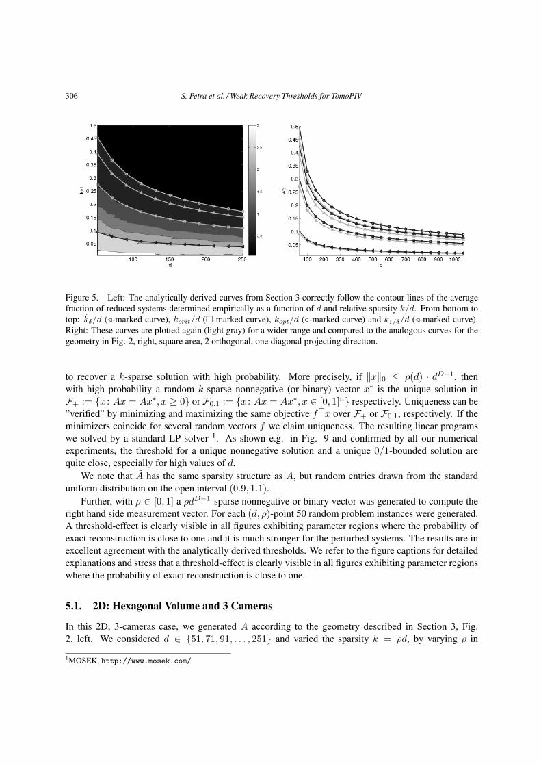
Figure 5. Left: The analytically derived curves from Section 3 correctly follow the contour lines of the averagefraction of reduced systems determined empirically as a function of d and relative sparsity k/d. From bottom totop: kδ/d (-marked curve), kcrit/d (-marked curve), kopt/d (-marked curve) and k1/δ/d (-marked curve).Right: These curves are plotted again (light gray) for a wider range and compared to the analogous curves for thegeometry in Fig. 2, right, square area, 2 orthogonal, one diagonal projecting direction.

to recover a k-sparse solution with high probability. More precisely, if x0 ≤ ρ(d) · dD−1, thenwith high probability a random k-sparse nonnegative (or binary) vector x∗ is the unique solution inF+ := x : Ax = Ax∗, x ≥ 0 or F0,1 := x : Ax = Ax∗, x ∈ [0, 1]n respectively. Uniqueness can be”verified” by minimizing and maximizing the same objective fx over F+ or F0,1, respectively. If theminimizers coincide for several random vectors f we claim uniqueness. The resulting linear programswe solved by a standard LP solver 1. As shown e.g. in Fig. 9 and confirmed by all our numericalexperiments, the threshold for a unique nonnegative solution and a unique 0/1-bounded solution arequite close, especially for high values of d.

We note that A has the same sparsity structure as A, but random entries drawn from the standarduniform distribution on the open interval (0.9, 1.1).

Further, with ρ ∈ [0, 1] a ρdD−1-sparse nonnegative or binary vector was generated to compute theright hand side measurement vector. For each (d, ρ)-point 50 random problem instances were generated.A threshold-effect is clearly visible in all figures exhibiting parameter regions where the probability ofexact reconstruction is close to one and it is much stronger for the perturbed systems. The results are inexcellent agreement with the analytically derived thresholds. We refer to the figure captions for detailedexplanations and stress that a threshold-effect is clearly visible in all figures exhibiting parameter regionswhere the probability of exact reconstruction is close to one.

5.1. 2D: Hexagonal Volume and 3 Cameras

In this 2D, 3-cameras case, we generated A according to the geometry described in Section 3, Fig.2, left. We considered d ∈ 51, 71, 91, . . . , 251 and varied the sparsity k = ρd, by varying ρ in

1MOSEK, http://www.mosek.com/


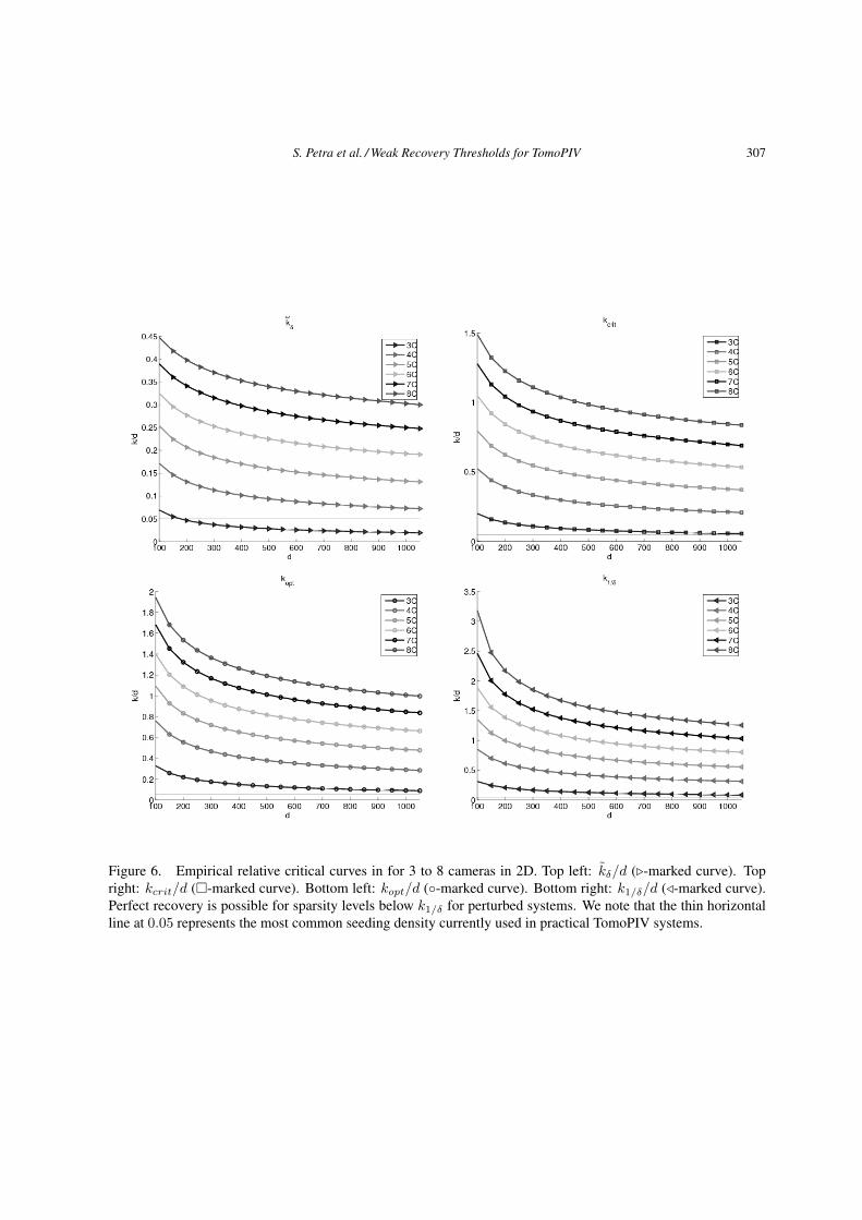
Figure 6. Empirical relative critical curves in for 3 to 8 cameras in 2D. Top left: kδ/d (-marked curve). Topright: kcrit/d (-marked curve). Bottom left: kopt/d (-marked curve). Bottom right: k1/δ/d (-marked curve).Perfect recovery is possible for sparsity levels below k1/δ for perturbed systems. We note that the thin horizontalline at 0.05 represents the most common seeding density currently used in practical TomoPIV systems.


Figure 7. Left: kopt/d (-marked curve) along with k1/δ/d (-marked curve). For 3 cameras k1/δ/d lies belowkopt/d, but starting with 5 cameras k1/δ significantly outperforms kopt. This shows the fundamental differencebetween the considered 0/1-matrices and random matrices underlying a symmetrical distribution with respect tothe origin. For random matrices recovery of k-sparse positive or binary vectors with sparsity levels beyond kopt

would be impossible. Right: For d = 200 the 6 curves depict the average ratio of mred(k)/nred(k) as a functionof sparsity k for 3 to 8 cameras from bottom to top.

Figure 8. Empirical recovery and non-recovery phase transitions for the 2D, 6 cameras case. Probability ofuniqueness in [0, 1]n of a k = ρd2 sparse binary vector for unperturbed (left) and perturbed matrices (right), alongwith kδ/d

2 (-marked curve), kcrit/d2 (-marked curve), kopt/d2 (-marked curve), and k1/δ/d2 (-marked

curve) from bottom to top. The dashed line depicts k/d2, with k solving mred(k) =2nred(k), which accurately

follows the border of the highly success area for all considered number of cameras, 3, 4 . . . 8. Recovery is possiblebeyond kopt, accurately described by k1/δ . In the 6 cameras case there is no evident performance boost for per-turbed systems, since the columns of reduced systems are most likely to be in general position for both perturbedand unperturbed systems. However, in the perturbed case recovery is more stable.


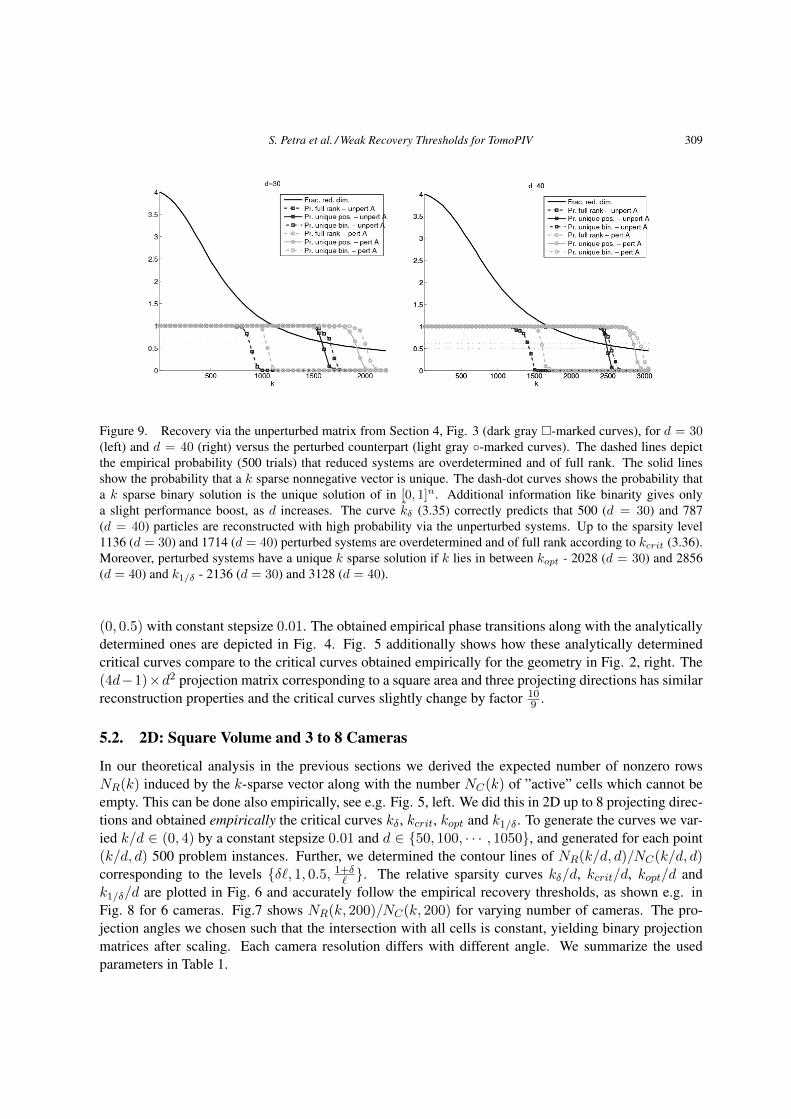
Figure 9. Recovery via the unperturbed matrix from Section 4, Fig. 3 (dark gray -marked curves), for d = 30(left) and d = 40 (right) versus the perturbed counterpart (light gray -marked curves). The dashed lines depictthe empirical probability (500 trials) that reduced systems are overdetermined and of full rank. The solid linesshow the probability that a k sparse nonnegative vector is unique. The dash-dot curves shows the probability thata k sparse binary solution is the unique solution of in [0, 1]n. Additional information like binarity gives onlya slight performance boost, as d increases. The curve kδ (3.35) correctly predicts that 500 (d = 30) and 787(d = 40) particles are reconstructed with high probability via the unperturbed systems. Up to the sparsity level1136 (d = 30) and 1714 (d = 40) perturbed systems are overdetermined and of full rank according to kcrit (3.36).Moreover, perturbed systems have a unique k sparse solution if k lies in between kopt - 2028 (d = 30) and 2856(d = 40) and k1/δ - 2136 (d = 30) and 3128 (d = 40).

(0, 0.5) with constant stepsize 0.01. The obtained empirical phase transitions along with the analyticallydetermined ones are depicted in Fig. 4. Fig. 5 additionally shows how these analytically determinedcritical curves compare to the critical curves obtained empirically for the geometry in Fig. 2, right. The(4d−1)×d2 projection matrix corresponding to a square area and three projecting directions has similarreconstruction properties and the critical curves slightly change by factor 10

9 .

5.2. 2D: Square Volume and 3 to 8 Cameras

In our theoretical analysis in the previous sections we derived the expected number of nonzero rowsNR(k) induced by the k-sparse vector along with the number NC(k) of ”active” cells which cannot beempty. This can be done also empirically, see e.g. Fig. 5, left. We did this in 2D up to 8 projecting direc-tions and obtained empirically the critical curves kδ, kcrit, kopt and k1/δ. To generate the curves we var-ied k/d ∈ (0, 4) by a constant stepsize 0.01 and d ∈ 50, 100, · · · , 1050, and generated for each point(k/d, d) 500 problem instances. Further, we determined the contour lines of NR(k/d, d)/NC(k/d, d)corresponding to the levels δ, 1, 0.5, 1+δ

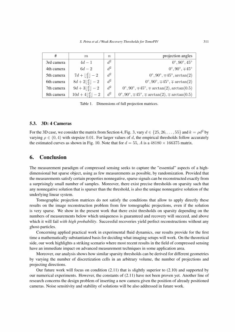
. The relative sparsity curves kδ/d, kcrit/d, kopt/d andk1/δ/d are plotted in Fig. 6 and accurately follow the empirical recovery thresholds, as shown e.g. inFig. 8 for 6 cameras. Fig.7 shows NR(k, 200)/NC(k, 200) for varying number of cameras. The pro-jection angles we chosen such that the intersection with all cells is constant, yielding binary projectionmatrices after scaling. Each camera resolution differs with different angle. We summarize the usedparameters in Table 1.


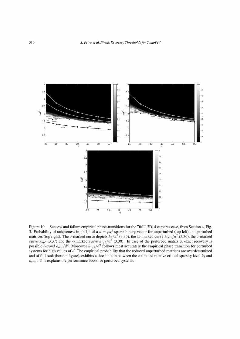
Figure 10. Success and failure empirical phase-transitions for the ”full” 3D, 4 cameras case, from Section 4, Fig.3. Probability of uniqueness in [0, 1]n of a k = ρd2 sparse binary vector for unperturbed (top left) and perturbedmatrices (top right). The -marked curve depicts kδ/d2 (3.35), the -marked curve kcrit/d

2 (3.36), the -markedcurve kopt (3.37) and the -marked curve k1/δ/d

2 (3.38). In case of the perturbed matrix A exact recovery ispossible beyond kopt/d

2. Moreover k1/δ/d2 follows most accurately the empirical phase transition for perturbedsystems for high values of d. The empirical probability that the reduced unperturbed matrices are overdeterminedand of full rank (bottom figure), exhibits a threshold in between the estimated relative critical sparsity level kδ andkcrit. This explains the performance boost for perturbed systems.


# m n projection angles3rd camera 4d− 1 d2 0, 90, 45

4th camera 6d− 2 d2 0, 90,∓45

5th camera 7d+ d2 − 2 d2 0, 90,∓45, arctan(2)

6th camera 8d+ 2d2 − 2 d2 0, 90,∓45,∓ arctan(2)

7th camera 9d+ 3d2 − 2 d2 0, 90,∓45,∓ arctan(2), arctan(0.5)

8th camera 10d+ 4d2 − 2 d2 0, 90,∓45,∓ arctan(2),∓ arctan(0.5)

Table 1. Dimensions of full projection matrices.

5.3. 3D: 4 Cameras

For the 3D case, we consider the matrix from Section 4, Fig. 3, vary d ∈ 25, 26, . . . , 55 and k = ρd2 byvarying ρ ∈ (0, 4) with stepsize 0.01. For larger values of d, the empirical thresholds follow accuratelythe estimated curves as shown in Fig. 10. Note that for d = 55, A is a 48180× 166375 matrix.

6. Conclusion

The measurement paradigm of compressed sensing seeks to capture the ”essential” aspects of a high-dimensional but sparse object, using as few measurements as possible, by randomization. Provided thatthe measurements satisfy certain properties nonnegative, sparse signals can be reconstructed exactly froma surprisingly small number of samples. Moreover, there exist precise thresholds on sparsity such thatany nonnegative solution that is sparser than the threshold, is also the unique nonnegative solution of theunderlying linear system.

Tomographic projection matrices do not satisfy the conditions that allow to apply directly theseresults on the image reconstruction problem from few tomographic projections, even if the solutionis very sparse. We show in the present work that there exist thresholds on sparsity depending on thenumbers of measurements below which uniqueness is guaranteed and recovery will succeed, and abovewhich it will fail with high probability. Successful recoveries yield perfect reconstructions without anyghost-particles.

Concerning applied practical work in experimental fluid dynamics, our results provide for the firsttime a mathematically substantiated basis for deciding what imaging setups will work. On the theoreticalside, our work highlights a striking scenario where most recent results in the field of compressed sensinghave an immediate impact on advanced measurement techniques in some application area.

Moreover, our analysis shows how similar sparsity thresholds can be derived for different geometriesby varying the number of discretization cells in an arbitrary volume, the number of projections andprojecting directions.

Our future work will focus on condition (2.11) that is slightly superior to (2.10) and supported byour numerical experiments. However, the constants of (2.11) have not been proven yet. Another line ofresearch concerns the design problem of inserting a new camera given the position of already positionedcameras. Noise sensitivity and stability of solutions will be also addressed in future work.


References[1] Azuma, K.: Weighted Sums of Certain Dependent Random Variables, Tohoku Math. J., 19(3), 1967, 357–

367.

[2] Berinde, R., Indyk, P.: Sparse Recovery Using Sparse Random Matrices, 2008, MIT-CSAIL TechnicalReport.

[3] Candes, E. J., Romberg, J., Tao, T.: Robust Uncertainty Principles: Exact Signal Reconstruction from HighlyIncomplete Frequency Information, IEEE Trans. Inf. Theor., 52(2), 2006, 489–509.

[4] DasGupta, A.: Asymptotic Theory of Statistics and Probability, Springer, 2008.

[5] Donoho, D.: Compressed Sensing, IEEE Trans. Inf. Theor.I, 52(4), 2006, 1289–1306.

[6] Donoho, D., Tanner, J.: Sparse Nonnegative Solution of Underdetermined Linear Equations by Linear Pro-gramming, Proc. National Academy of Sciences, 102(27), 2005, 9446–9451.

[7] Donoho, D., Tanner, J.: Counting the Faces of Randomly-Projected Hypercubes and Orthants, with Applica-tions, Discrete Comput. Geom., 43(3), 2010, 522–541.

[8] Donoho, D., Tanner, J.: Precise Undersampling Theorems, Proceedings of the IEEE, 98(6), 2010, 913–924,ISSN 0018-9219.

[9] Elsinga, G., Scarano, F., Wieneke, B., van Oudheusden, B.: Tomographic Particle Image Velocimetry,Exp. Fluids, 41, 2007, 933–947.

[10] G.T. Herman, G., Kuba, A.: Discrete Tomography: Foundations, Algorithms and Applications, Birkhauser,1999.

[11] Khajehnejad, M., Dimakis, A., Xu, W., Hassibi, B.: Sparse Recovery of Positive Signals with MinimalExpansion, IEEE Trans. Sig. Proc., 59, 2011, 196–208.

[12] Mangasarian, O., Recht, B.: Probability of Unique Integer Solution to a System of Linear Equations, Eur. JOper. Res., 214(1), 2011, 27–30.

[13] Petra, S., Schnorr, C.: TomoPIV meets Compressed Sensing, Pure Math. Appl., 20(1-2), 2009, 49–76.

[14] Petra, S., Schnorr, C.: Average Case Recovery Analysis of Tomographic Compressive Sensing,arXiv:1208.5894v2 [math.NA], August 30 2012.

[15] Petra, S., Schroder, A., Schnorr, C.: 3D Tomography from Few Projections in Experimental Fluid Mechanics,in: Imaging Measurement Methods for Flow Analysis (W. Nitsche, C. Dobriloff, Eds.), vol. 106 of Notes onNumerical Fluid Mechanics and Multidisciplinary Design, Springer, 2009, 63–72.

[16] Vlasenko, A., Schnorr, C.: Variational Approaches for Model-Based PIV and Visual Fluid Analysis, in:Imaging Measurement Methods for Flow Analysis (W. Nitsche, C. Dobriloff, Eds.), vol. 106 of Notes onNumerical Fluid Mechanics and Multidisciplinary Design, Springer, 2009, 247–256.

[17] Wang, M., Xu, W., Tang, A.: A Unique ”Nonnegative” Solution to an Underdetermined System: FromVectors to Matrices, IEEE Trans. Sig. Proc., 59(3), 2011, 1007–1016.

[18] Wendel, J.: A Problem in Geometric Probability, Math. Scand., 11, 1962, 109–111.

[19] Xu, W., Hassibi, B.: Efficient Compressive Sensing with Deterministic Guarantees Using Expander Graphs,Information Theory Workshop, 2007. ITW ’07. IEEE, 2007.

Documents

Critical Parameter Values and Reconstruction Propertiesof Discrete