Cosmological Perturbation Theory and Structure Formationcds.cern.ch/record/484698/files/0101009.pdf · Cosmological Perturbation Theory and Structure ... treatment of large scale

COSMOLOGY 2000Conference ProceedingsM. C. Bento, O. Bertolami, L. Teodoro, eds.

Cosmological Perturbation Theory and StructureFormation

Edmund Bertschinger

Department of Physics, MIT Room 6-207, 77 Massachusetts Avenue,Cambridge, MA 02139, USA

Abstract. These lecture notes discuss several topics in the physics ofcosmic structure formation starting from the evolution of small-amplitudefluctuations in the radiation-dominated era. The topics include relativis-tic cosmological perturbation theory with the scalar-vector-tensor decom-position, the evolution of adiabatic and isocurvature initial fluctuations,microwave background anisotropy, spatial and angular power spectra, thecold dark matter linear transfer function, Press-Schechter theory, and abrief introduction to numerical simulation methods.

1. Introduction

The advent of precision cosmology with measurements of the Cosmic MicrowaveBackground (CMB) radiation has brought a new focus on the physics of the z >1100 universe. The connection between two fossil relics of the early universe—CMB fluctuations and galaxies—offers the possibility for improved understand-ing of both as well as tighter constraints on cosmological parameters. Theselectures present an overview of the physics of structure formation starting af-ter the inflationary epoch, going through recombination, and extending to thepresent day.

Cosmological perturbation theory is often regarded as a highly technicalsubject beyond the scope of graduate courses in cosmology. However, these lec-tures may suggest how, with minor simplification, it can be integrated into atreatment of large scale structure. The potential benefits are many—a detailedunderstanding of CMB anisotropy, a quantitative explanation for the key fea-tures of the cold dark matter transfer function, and an extension of the intuitiondeveloped from the Newtonian theory of large scale structure to the physics ofthe post-inflationary universe. The aim of the current notes is more modest,but it is hoped that they provide some direction for those wishing to delve moredeeply into cosmological perturbation theory and structure formation.

2. Overview of Relativistic Cosmological Perturbation Theory

The goal of cosmological perturbation theory is to relate the physics of the earlyuniverse (e.g. inflation) to CMB anisotropy and large-scale structure and toprovide the initial conditions for numerical simulations of structure formation.The physics during the period from the end of inflation to the beginning of

1

2 Edmund Bertschinger

nonlinear gravitational collapse is complicated by relativistic effects but greatlysimplified by the small amplitude of perturbations. Thus, an essentially completeand accurate treatment of relativistic perturbation evolution is possible, at leastin the context of simple fluctuation models like inflation. Numerous articleshave been written on this topic. See [1, 2] for references and for more detailedtreatments similar in style to the present lecture notes.

The starting point for cosmological perturbation theory is the metric of aperturbed Robertson-Walker spacetime,

ds2 =[g(0)µν + g(1)

µν

]dxµdxν

= a2(τ)[−dτ2 + γij(~x )dxidxj + hµν(~x, τ)dxµdxν

]. (1)

Spatial coordinates take the range 1 ≤ i, j ≤ 3; xi (or ~x for all three) is acomoving spatial coordinate; τ is conformal time; a(τ) is the cosmic expansionscale factor; units are chosen so that the speed of light is unity; and γij(~x ) is the3-metric of a maximally symmetric constant curvature space. Conformal timeis related to the proper time measured by a comoving observer (i.e. one at fixed~x) by dt = a(τ)dτ . For cosmological perturbation theory it is more convenientthan proper time. The metric perturbations are given by hµν = g

(1)µν /a2.

The Robertson-Walker model is characterized by one function of time, a(τ),and one constant, the curvature constant K. The expansion factor obeys theFriedmann equation, (

a

a

)2

=8π3Ga2ρ(a)−K (2)

where a dot denotes d/dτ and ρ(a) is the total mean energy density. Note thatthe usual Hubble parameter is H = a/a2.

The spatial part of the Robertson-Walker metric takes a simple form inspherical coordinates (χ, θ, φ):

γijdxidxj = dχ2 + r2(χ)

(dθ2 + sin2 θdφ2

). (3)

The angular radius r(χ) takes one of three forms depending on the sign of K:

r(χ) =

1√K

sin(χ√K), K > 0,

χ, K = 0,1√−K

sinh(χ√−K), K < 0 .

(4)

These cases are referred to as closed, flat, and open, respectively. Many authorschoose units of length such that χ = ±1 or 0. However, it is convenient to let Khave units (inverse length squared). From the Friedmann equation, K = (Ω0 −1)H2

0 where the subscript 0 denotes the present value and Ω0 is the total densityparameter (including dark energy). Note that the range of χ is [0,∞) in theflat and open models but is [0, π/

√K] in the closed model. The flat Robertson-

Walker model favored by inflation is conformal to Minkowski spacetime, i.e. themetrics are identical up to an overall conformal factor a2(τ).

Cosmological Perturbation Theory and Structure Formation 3

2.1. Scalar-Vector-Tensor Decomposition

In linear perturbation theory, the metric perturbations hµν are regarded as atensor field residing on the background Robertson-Walker spacetime. As a sym-metric 4 × 4 matrix, hµν has 10 degrees of freedom. Because of the ability tomake continuous deformations of the coordinates, 4 of these degrees of freedomare gauge- (coordinate-) dependent, leaving 6 physical degrees of freedom. Aproper treatment of cosmological perturbation theory requires clear separationbetween physical and gauge degrees of freedom.

The metric degrees of freedom in linear pertubation theory were classifiedby Lifshitz in 1946 [3]. Lifshitz presented the scalar-vector-tensor decompositionof the metric. It is based on a 3 + 1 split of the components, which we rewriteas follows:

h00 ≡ −2ψ , h0i ≡ wi , hij = 2 (φγij + Sij) with γijSij = 0. (5)

Here, γij is the matrix inverse of γij . The trace part of hij has been absorbedinto φ so that Sij has only 5 independent components.

With the space-time (3 + 1) split, we use γij (or γij) to lower (or raise)indices of spatial 3-vectors and tensors. For convenience, spatial derivatives willbe written using the 3-dimensional covariant derivative ∇i defined with respectto the 3-metric γij ; it is a three-dimensional version of the full 4-dimensionalcovariant derivative presented in general relativity textbooks. For example, ifK = 0, we can choose Cartesian coordinates such that γij = δij and ∇i = ∂/∂xi.

The scalar-tensor-vector split is based on the decomposition of a vectorinto longitudinal and transverse parts. For any three-vector field wi(~x ), we maywrite

wi = w‖i + w⊥i where ~∇× ~w ‖ = ~∇ · ~w⊥ = 0 . (6)

The curl and divergence are defined using the spatial covariant derivative, e.g.~∇ · ~w = γij∇iwj.

The longitudinal/transverse decomposition is not unique (e.g. one mayalways add a constant to w‖i ) but it always exists. The terminology arises becausein the Fourier domain w

‖i is parallel to the wavevector while w⊥i is transverse

(perpendicular to the wavevector). Note that w‖i = ∇iφw for some scalar fieldφw. Thus, the longitudinal/transverse decomposition allows us to write a vectorfield in terms of a scalar (the longitudinal or irrotational part) and a part thatcannot be obtained from a scalar (the transverse or rotational part).

A similar decomposition holds for a two-index tensor, but now each indexcan be either longitudinal or transverse. For a symmetric tensor, there arethree possibilities: both indices are longitudinal, one is transverse, or two aretransverse. These are written as follows:

Sij = S‖ij + S⊥ij + ST

ij , (7)

whereγjk∇kSij = γjk∇kS

‖ij + γjk∇kS

⊥ij . (8)

The first term in equation (8) is a longitudinal vector while the second term isa transverse vector. The divergence of the doubly-transverse part, ST

ij, is zero.


For a traceless symmetric tensor, the doubly and singly longitudinal parts canbe obtained from the gradients of a scalar and a transverse vector, respectively:

S‖ij =

(∇i∇j − 1

3γij∇2

)φS , S⊥ij = ∇iS

⊥j +∇jS

⊥i . (9)

Although we will not prove it here (see [1] for the details), under an in-finitesimal coordinate transformation S

‖ij and S⊥ij can change while ST

ij is in-variant. Similarly, the longitudinal and transverse parts of wi = h0i are bothgauge-dependent.

Now we have the mathematical background needed to perform the scalar-tensor-vector split of the physical degrees of freedom of the metric. The “tensormode” represents the part of hij that cannot be obtained from the gradients ofa scalar or vector, namely ST

ij . The tensor mode is gauge-invariant and has twodegrees of freedom (five for a symmetric traceless 3 × 3 matrix, less three fromthe condition γjk∇kS

Tij = 0). Physically it represents gravitational radiation;

the two degrees of freedom correspond to the two polarizations of gravitationalradiation. Gravitational radiation is transverse: a wave propagating in the z-direction can have nonzero components hxx − hyy and hxy = hyx but no others.The tensor mode ST

ij behaves like a spin-2 field under spatial rotations. Notethat my definition of the tensor mode strain Sij here differs by a factor of 2 fromthe conventional hTT

ij in [4].The “vector mode” behaves like a spin-1 field under spatial rotations. It

corresponds to the transverse vector parts of the metric, which are found in w⊥iand S⊥ij . Each part has two degrees of freedom. Although we will not prove ithere (see [1] for the details), it is possible to eliminate two of these degrees offreedom by imposing gauge conditions (coordinate conditions). The synchronousgauge of Lifshitz [3] is one popular choice, with w⊥i = w

‖i = 0. Another choice

is the “Poisson” or transverse gauge [1] which sets S⊥ij = 0. In either case,there are two physical degrees of freedom and they correspond physically togravitomagnetism. Although this effect is less well known than gravitationalradiation or Newtonian gravity, it produces magnetic-like effects on moving andspinning masses, such as the precession of a gyroscope in the gravitational fieldof a spinning mass (Lense-Thirring precession). This phenomenon has not yetbeen discovered experimentally but should be measured by the Gravity ProbeB satellite to be launched in 2002 [5].

The “scalar mode” is spin-0 under spatial rotations and corresponds physi-cally to Newtonian gravitation with relativistic modifications. The scalar partsof the metric are given by φ, ψ, w‖i , and S‖ij. Any two of these may be set to zero

by means of a gauge transformation. One popular choice is w‖i = S‖ij = 0, also

known as the conformal Newtonian gauge. It corresponds to the scalar mode inthe transverse gauge, defined by the gauge conditions

γij∇iwj = 0 , γjk∇kSij = 0 . (10)

This gauge in linearized general relativity is the gravitational analogue of Coulombgauge in electromagnetism, where the magnetic vector potential is transverse,


∇iAi = 0. In the gravitational transverse gauge, wi is transverse and Sij is dou-

bly transverse. This gauge is convenient for developing intuition although notnecessarily the best for computation. The variables (φ,ψ,w⊥i , S

Tij) correspond

to gauge-invariant variables introduced by Bardeen [6] as linear combinations ofmetric variables in other gauges.

In linear perturbation theory, the scalar, vector, and tensor modes evolveindependently. The vector and tensor modes produce no density perturbationsand therefore are unimportant for structure formation, although they do perturbthe microwave background. In the remainder of these lectures, only the scalarmode will be considered.

The Einstein equations give the equations of motion for the metric per-turbations in terms of the energy-momentum tensor, the source of relativisticgravity. Here we consider the case of a perfect fluid (or several perfect fluidcomponents combined), for which

T µν = (ρ+ p)V µV ν + pgµν (11)

where ρ and p are the proper energy density and pressure in the fluid rest frameand V µ is the fluid 4-velocity.

We split T µν into time and space components as we did for the metric. Itis convenient to use mixed components because the conformal factor a2 thencancels, yielding

T 00 = −ρ(~x, τ) = − [ρ(τ) + δρ(~x, τ)] ,

T 0i = [ρ(τ) + p(τ)] vi(~x, τ) = − [ρ(τ) + p(τ)]∇iW , (12)

T ij = [p(τ) + δp(~x, τ)] δi

j ,

where ρ(τ) and p(τ) are respectively the energy (or mass) density and pres-sure of the Robertson-Walker background spacetime, vi = γijdx

j/dτ is the fluid3-velocity (assumed nonrelativistic), and W is a velocity potential. We are as-suming that the velocity field is irrotational or, if it is not, that the matterfluctuations are linear so that the longitudinal and transverse velocity compo-nents evolve independently. This is a good approximation prior to the epoch ofgalaxy formation.

We are also making another approximation, namely that the shear stress(the non-diagonal part of T i

j) is negligible compared with the pressure. Thisis a bad approximation for relativistic neutrinos, whose free-streaming leads toa non-isotropic momentum distribution after neutrino decoupling at a tempera-ture of about 1 MeV. (A similar but smaller effect occurs for photons after theydecouple at a temperature of about 0.3 eV.) However, the effect of this erroris modest during the radiation-dominated era (photons contribute more pres-sure than neutrinos, and are isotropic) and is unimportant during the matter-dominated era, when the nonrelativistic matter density is the major source ofgravity. We introduce this approximation here in order to simplify the treat-ment; full calculations include the effects of neutrino shear stress [2].

When the stress tensor is isotropic, the Einstein equations in transversegauge imply that the two scalar potentials φ and ψ are equal [1] and the metrictakes the simple form

ds2 = a2(τ)[−(1 + 2φ)dτ2 + (1− 2φ)γijdx

idxj]. (13)


This is a simple cosmological generalization of the standard weak-field limit ofgeneral relativity, which is recovered by setting a = 1 and γij = δij .

Given the stress-energy tensor, we can now obtain field equations for φ(~x, τ)using the Einstein equations. The only independent equation for the Robertson-Walker background is the Friedmann equation (2). For the perturbations, weobtain

(∇2 + 3K)φ = 4πGa2[δρ+ 3

a

a(ρ+ p)W

], (14)

∂τφ+a

aφ = 4πGa2(ρ+ p)W , (15)

and∂2

τφ+ 3a

a∂τφ−

(8πGa2p+ 2K

)φ = 4πGa2δp . (16)

There are more equations than in Newtonian gravity because the Einstein equa-tions have local energy-momentum conservation built into them.

Equation (14) is remarkably like the Poisson equation of Newtonian grav-ity, especially when one realizes that the factor of a2 is needed to convert theLaplacian from comoving to proper spatial coordinates. Otherwise there arethree differences. First, the spatial curvature adds a scale to the Laplacian in acurved space. Second, the density source is δρ = ρ − ρ rather than ρ becauseφ represents a metric perturbation on top of the background Robertson-Walkerspacetime. Third, momentum density (through W ) is a source for gravity ingeneral relativity. However, this term is comparable with the density term onlyon length scales comparable to or larger than the Hubble length H−1.

Two of our field equations are unfamiliar from Newtonian dynamics. Equa-tion (15) is reminiscent of the Zel’dovich approximation [7] in that the velocitypotential is proportional to the gravitational potential in the linear regime whenφ(~x, τ) = φ0(~x )Dφ(τ). However, it is a more general result whose Newtonianlimit may be derived by combining the continuity equation with the time deriva-tive of the Poisson equation.

Equation (16) is more surprising, as it gives the gravitational potentialthrough a second-order time evolution equation as opposed to the action-at-a-distance Poisson equation (14). The reader may well wonder about the com-patibility of the two equations as well as the physical validity of the Poissonequation in general relativity, but equations (14)–(16) are all correct. See [1]for a full discussion. In brief, causality is restored by the tensor mode. Thetime evolution equation for the potential can be regarded as arising from localenergy-momentum conservation (which is built into the Einstein equations) com-bined with the Poisson equation. Indeed, an equation similar to equation (16)can be derived in Newtonian gravity from the fluid and Poisson equations. Itsutility arises from the fact that when pressure perturbations are gravitationallyunimportant (i.e. when matter and/or dark energy dominate over radiation),the time evolution of perturbations can be obtained from a single differentialequation depending only on the background curvature, pressure, and density.

2.2. Perfect Fluid Model

To conclude this section, we present a simple model for understanding CMBanisotropy and large scale structure. We reduce the matter and energy content


of the universe to a vacuum energy (with ρv = Λ/8πG contributing to the meanexpansion rate but not to the fluctuations) and two fluctuating components,CDM and radiation (photons and neutrinos, the former coupled to baryons byelectron scattering until recombination). The CDM and radiation are treatedas perfect fluids, ignoring the free-streaming of neutrinos and the diffusion andstreaming of photons during and after recombination.

The fluid equations follow from local energy-momentum conservation, ∇µTµν =

0. For a perfect fluid, with the scalar mode only (no vorticity and no gravita-tional radiation), the fluid equations in the metric of equation (13) are

∂τρ+ 3(a

a− ∂τφ

)(ρ+ p) +∇i

[(ρ+ p)vi

]= 0 (17)

and∂τ

[(ρ+ p)vi

]+ 4

a

a(ρ+ p)vi +∇ip+ (ρ+ p)∇iφ = 0 . (18)

These are familiar from Newtonian fluid dynamics, with some extra terms. Thedamping (a/a) terms arise from Hubble expansion and the use of comovingcoordinates. The ∂τφ term in the continuity equation (17) arises from the de-formation of the spatial coordinates, i.e. the φδij contribution to the metric.(The flux term in eq. 17 describes transport relative to the comoving coordi-nate grid, which is deforming when ∂τφ 6= 0.) The energy flux (or momentumdensity, they are equal) includes pressure in relativity because of the pdV workdone by compression. Equations (17) and (18) apply separately to perfect fluidcomponent.

3. Adiabatic and Isocurvature Modes

This section discusses the evolution of perturbations from the end of inflation(taken to be at τ = 0 for all practical purposes) through recombination using atwo-fluid approximation. We approximate the matter and energy content in theuniverse as being two perfect fluids: Cold Dark Matter (a zero-temperature gas)and radiation (photons coupled to electrons and baryons before recombination,plus neutrinos which are approximated as behaving like photons). The netenergy density perturbation is thus

δρ(~x, τ) = ρc(a)δc(~x, τ) + ρr(a)δr(~x, τ) , (19)

where ρc ∝ a−3 and, if we neglect the contribution of baryons, ρr ∝ a−4. Wecould add a third component for the baryons, but this complicates the presen-tation without adding essential new behavior. In the interest of economy, weleave baryons out. We define the relative density contrasts δc ≡ δρc/ρc andδr ≡ δρr/ρr.

The total pressure is simply p(~x, τ) = 13 ρr(a)(1 + δr) + pv where pv =

−ρv is the spatially constant negative pressure of vacuum energy (cosmologicalconstant), should any be present.

As we noted in the previous section, density perturbations couple gravita-tionally only to the scalar mode of metric perturbations, and the scalar modecannot generate transverse vector fields. As a result, the peculiar velocity fields


of CDM and radiation are longitudinal and are fully characterized by their po-tentials Wc and Wr for CDM and radiation, respectively.

As a final simplifying assumption, we will assume that we are studying ef-fects on distance scales less than the curvature length |K|−1/2 = |Ω0−1|−1/2H−1

0 ,which is at least 5 Gpc and possibly infinitely large.

With these assumptions, we can linearize the fluid equations (17) and (18)for δ2c 1 and δ2r 1 to obtain

∂τ δc = ∇2Wc + 3∂τφ , ∂τδr =43∇2Wr + 4∂τφ ,

∂τWc +a

aWc = φ , ∂τWr =

14δr + φ . (20)

These equations are easy to understand. The ∂τφ terms have the same ori-gin as in equation (17), namely the deformation of the comoving coordinatesystem. The velocity potential terms are related to the velocity divergence,~∇ · ~v = −∇2W . The radiation density fluctuations grow at 4/3 the rate ofmatter fluctuations to compensate for the fact that the photon number densityis proportional to ρ3/4

r . As expected, the velocity equations show that mattervelocities redshift (for φ = 0) with ~vc ∝ a−1 while radiation velocities (e.g. thespeed of light) do not redshift. (Momenta redshift ∝ a−1 but the speed of lightis unaffected by expansion.) Finally, radiation pressure gives rise to an acousticrestoring force −~∇pr = −(1/3)ρr

~∇δr which shows up as the (1/4)δr term in theradiation longitudinal velocity equation.

Equations (20) are coupled by gravity, which can be determined from thePoisson equation (14), which becomes

∇2φ = 4πGa2[(ρrδr + ρcδc) +

a

a(4ρrWr + 3ρcWc)

]. (21)

We can solve equations (20) and (21) most easily by expanding the spatialdependence in eigenfunctions of the Laplacian ∇2. In flat space these are planewaves exp(i~k · ~x ), and this is a good approximation even if the background iscurved, provided k |K|1/2. This approximation is valid for almost all appli-cations except large angular scale CMB anisotropy. Note that ~k is a comovingwavevector; the physical wavelength is 2πa/k.

By expanding the spatial dependence in plane waves, we now have a fourth-order linear system of ordinary differential equations in time. We are free todefine linear combinations of the variables (δc, δr,Wc,Wr) as our fundamentalvariables. In terms of the mechanisms for generating primeval perturbations, themost natural variables are the metric perturbation φ and the specific entropy

η ≡ δp − c2s δρ

ρcc2s=

34δr − δc , (22)

where

c2s ≡dp/dτ

dρ/dτ=[3(

1 +3ρc

4ρr

)]−1

(23)


is the effective one-fluid sound speed of the matter and radiation. (Acousticsignals actually do not propagate at this speed; they propagate with speed 3−1/2

through the radiation and they do not propagate at all through CDM.)For a two-component radiation plus CDM universe, the solution of the

Friedmann equation (2) gives

y ≡ ρc

ρr=a(τ)aeq

=τ

τe+(τ

2τe

)2

, τe ≡(aeq

Ωc

)1/2

H−10 =

19MpcΩch2

. (24)

The radiation-dominated era ends and matter-dominated era begins at redshift1+zeq = a−1

eq = 2.5×104Ωmh2. A cosmological constant has no significant effect

on y(τ) provided that, during the times of interest, the vacuum energy densityis much less than the radiation or cold dark matter density.

The fluid and Poisson equations can now be combined to give a pair ofsecond-order ordinary differential equations,

13c2s

∂2τφ+

(1 +

1c2s

)a

a∂τφ+

(k2

3+

14yτ2

e

)φ =

η

2yτ2e

,

13c2s

∂2τ η +

a

a∂τη +

k2y

4η =

16y2k4τ2

e φ . (25)

It is interesting to note that φ and η evolve independently aside from the sourceterm each provides to the other. The coupling implies that entropy perturbationsare a source for the growth of gravitational perturbations and vice versa.

For a given wavenumber k, there are two key times in the evolution of φand η: the sound-crossing time τ ≈ π/(kcs) and the time of matter-radiationequality at τ ≈ τe. [To be precise, a = aeq at τ/τe = 2(

√2 − 1).] For τ τe, φ

and η decouple and they both have solutions that decay rapidly with τ as well assolutions that are finite as τ → 0. The latter are conventionally called “growingmodes” while the former are called decaying. The growing mode solution in theradiation era τ τe is

φ(~k, τ) =3

(ωτ)3(sinωτ − ωτ cosωτ)A(~k )

+τ

τe

[1

(ωτ)4+

12(ωτ)2

− 1(ωτ)4

(cos ωτ + ωτ sinωτ)]I(~k ) , (26)

η(~k, τ) = I(~k ) + 9[lnωτ + C − Ci(ωτ) +

12(cosωτ − 1)

]A(~k ) ,

where ω ≡ k/√

3 is the phase of acoustic waves in the radiation fluid, C =0.5772 . . . is the Euler constant, and Ci(x) is the cosine integral defined by

Ci(x) = C + lnx+∫ x

0

cos t− 1t

dt . (27)

In equation (26) we have neglected all terms O(τ/τe) aside from the lowest-ordercontribution of I(~k ) to φ.


The general growing-mode solution contains two k-dependent integrationconstants, A(~k ) and I(~k ), which represent the initial (τ → 0) amplitude ofφ and η, respectively. Conventionally they are called the “adiabatic” (so-calledbecause the entropy perturbation η = 0 at τ = 0, although “isentropic” would bemore appropriate) and “isocurvature” (so-called because φ = 0 at τ = 0) modeamplitudes. In addition, there are decaying modes whose amplitude at τ = τeis negligible unless the initial conditions were fine-tuned or there are externalsources such as topological defects to continually regenerate the decaying mode.The solution of equations (26) is valid only for inflation or other mechanisms thatgenerate fluctuations exclusively in the early universe, but not for topologicaldefects.

As a result of reheating, inflation produces fluctuations with spatially con-stant ratios of the number densities of all particle species. For CDM and ra-diation, for example, ρ3/4

r /ρc = constant hence I = 0 and thus η = 0 untilradiation pressure forces begin to separate the radiation from the CDM, whichtakes a sound-crossing time or τ ∼ ω−1. Thus, although inflation produces theadiabatic mode of initial fluctuations, the differing equations of state p(ρ) forthe two-fluid system lead to entropy perturbations proportional to the initialadiabatic mode amplitude A(~k ) (see the second of eqs. 26).

Physically, the number density of particles of all species are proportional toeach other in the adiabatic mode as long as there has been too little time forparticles to travel a significant difference via their thermal speeds. However, thediffering thermal speeds of different particle species (e.g. photons and cold darkmatter) eventually cause the particle densities to evolve differently, so that thenumber density ratios are no longer constant and the entropy perturbation is nolonger zero.

First-order phase transitions, on the other hand, change the equation ofstate without moving matter or energy on macroscopic scales, hence δρr + δρc =θc = θr = 0 initially implying φ = 0 initially but η 6= 0. This isocurvature modeis characterized by the initial entropy perturbation amplitude I(~k ). As the firstof equations (26) shows, the isocurvature mode generates curvature fluctuationswhen the universe becomes matter-dominated.

The isocurvature CDM inflationary model has a fine balance such thatδr + yδc = 0 initially. This may involve nonlinear fluctuations of δc at earlytimes, but δr is negligible early in the radiation-dominated era y 1. For thisreason, the isocurvature mode was originally called isothermal [8].

On small scales, kτ 1, equations (25) may be solved using a WKBapproximation. For our purposes it suffices to take the ωτ 1 limit of equations(26):

φ ≈ −3cosωτ(ωτ)2

A(~k ) +1

ω3τeτ2

(ωτ

2− sinωτ

)I(~k ) . (28)

The radiation density fluctuation scales as

δr ∼ k2φ

Ga2ρr∼ k2τ2φ ,

which oscillates in proportion to cosωτ for the adiabatic mode and grows inproportion to y ∼ τ/τe for the isocurvature mode.


Note from equation (28) that the isocurvature mode induces oscillations inthe potential with a π/2 phase shift relative to the adiabatic mode. This shifttranslates into a shift in the positions of the acoustic peaks in the CMB angularpower spectrum.

3.1. The Adbiabatic Growing Mode as a Standing Wave

It is instructive to consider the general adiabatic perturbation in the radiation-dominated era including the decaying mode. This problem is easy to analyzeand shows the role of acoustic waves in the radiation-dominated era.

The two linearly independent solutions of the first of equations (25) fory 1 and adiabatic initial conditions (η = 0) are

φg =3

(ωτ)3(sinωτ − ωτ cosωτ) , φd =

3(ωτ)3

(cos ωτ + ωτ sinωτ) (29)

where the subscripts label the growing and decaying modes, respectively. Theyare the real and imaginary parts of

φω = φg + iφd =3

(ωτ)3(i− ωτ)e−iωτ . (30)

For a given spatial harmonic, exp(i~k ·~x )φω represents a wave traveling in the~k-direction. Thus, the growing mode φg = 1

2 (φω +φ∗ω) represents a superpositionof waves traveling along ~k and −~k, i.e. a standing wave

φg cos kx = Re 32(ωτ)3

[(i− ωτ)ei(~k·~x−ωτ) + (−i− ωτ)ei(~k·~x+ωτ)

]. (31)

The waves travel at the sound speed ω/k = 1/√

3 in the radiation fluid.The entropy perturbation induced by a traveling wave potential perturba-

tion is easily calculated in the radiation-dominated era using the Green’s functionmethod applied to the second of equations (25) with φ = φω for the source term.The result is

ηω = 9∫ ωτ

0

1x

(1− e−ix

)dx− 9

2

(1− e−iωτ

). (32)

The real part of this equation gives the A(~k ) contribution to η in equations (26).

4. CMB Anisotropy

This section presents a simplified treatment of CMB anisotropy, with the aim ofhighlighting the essential physics without getting lost in all of the details. Morecomplete treatments are found in [9, 10].

The microwave background radiation is fully described by a set of photonphase space distribution functions. Ignoring polarization (a few percent effect),all the information is included in the intensity or in f(~x, ~p, τ) where fd3p isthe number density of photons of conjugate momentum ~p at position and time


(~x, τ). The conjugate momentum is related to the proper momentum measuredby a comoving observer, ~p/a, so that ~p = constant along a photon trajectory inthe absence of metric perturbations.

Remarkably, despite metric perturbations and scattering with free electrons,the CMB photon phase space distribution remains blackbody (Planckian) toexquisite precision:

f(~x, ~p, τ) = fPlanck

(E

kT

)= fPlanck

[p

kT0(1 + ∆)

](33)

where T0 = 2.728 K is the current CMB temperature and ∆(~x, ~n, τ) is thetemperature variation at position (~x, τ) for photons traveling in direction ~n.The phase space density is blackbody but the temperature depends on photondirection as a result of scattering and gravitational processes occurring alongthe line of sight.

The phase space density may be calculated from initial conditions in theearly universe through the Boltzmann equation

Df

Dτ≡ ∂f

∂τ+∂f

∂~x· d~xdτ

+∂f

∂~p· d~pdτ

=(df

dτ

)c

(34)

where the right-hand side is a collision integral coming from nonrelativisticelectron-photon elastic scattering. In the absence of scattering, the phase spacedensity is conserved along the trajectories

d~x

dτ= ~n ≡ ~p

p,

1p

dp

dτ= −~n · ~∇φ+ ∂τφ ,

d~n

dτ= −2

[~∇− ~n (~n · ~∇)

]φ . (35)

Note that the photon energy changes via gravitational redshift (the first term indp/dτ ) or a time-changing potential, but in either case the energy of all photonsis changed by the same factor. The photon direction changes by transversedeflections due to gravity; d~n/dτ is twice the Newtonian value, a result well-known in gravitational lens theory [11]. Because ∂f/∂~n = 0 for the unperturbedbackground (the anisotropy arises due to the metric perturbations), gravitationallensing affects the CMB anisotropy only through nonlinear effects on small scales[12].

The procedure for computing CMB anisotropy is to linearize the Boltzmannequation assuming ∆2 1 [13]. Until recently, the temperature anisotropy ∆was expanded in spherical harmonics and the Boltzmann equation was solvedas a hierarchy of coupled equations for the various angular moments [2]. In1996, Seljak and Zaldarriaga [9] developed a much faster integration methodcall CMBFAST based on integrating the linearized Boltzmann equation alongthe observer’s line of sight before the angular expansion is made:

∆(~n, τ0) =∫ τ0

0dχ e−τT(χ)

[−~n · ~∇φ+ ∂τφ+ aneσT

(14δγ + ~ve · ~n+ pol. term

)]ret

(36)where τ0 is the present conformal time, χ is the radial comoving coordinate ofequation (3), subscript “ret” denotes evaluation using retarded time τ = τ0−χ,δγ is the relative density fluctuation in the photon gas (δγ = δr in our two-fluid


approximation), ~ve is the mean electron velocity (i.e. the baryon velocity, whichequals ~vr in our two-fluid approximation), σT is the Thomson cross section, andthe Thomson optical depth is

τT(χ) ≡∫ χ

0dχ (aneσT)ret . (37)

We have left out small terms (“pol. term”) due to polarization and the anisotropyof Thomson scattering in equation (36).

The terms in equation (36) are easy to understand. The exp(−τT) factoraccounts for the opacity of electron scattering, which prevents us from seeingmuch beyond a redshift of 1100, where τT ≈ 1. The CMB anisotropy appears tocome from a thin layer called the photosphere, just like the radiation from thesurface of a star.

The two gravity terms give the effective emissivity due to the photon energychange caused by a varying gravitational potential. For a blackbody distribution,if all photon energies are increased by a factor 1 + ε, the distribution remainsblackbody with a temperature increased by the same factor. Thus, the line-of-sight integration of the fractional energy change of equation (35) translatesdirectly into a temperature variation.

The terms proportional to the Thomson opacity aneσT are the effectiveemissivity due to Thomson scattering. Bearing in mind that the photon-baryonplasma is in nearly perfect thermal equilibrium (the temperature variations areonly about 1 part in 105), the photons we see scattered into the line of sightfrom a given fluid element have the blackbody distribution corresponding to thetemperature of that element. Recalling that the energy density of blackbodyradiation is ργ ∝ T 4, we see that 1

4δγ is simply the fractional temperaturevariation of the fluid element. In other words, if we carried a thermometerto the photosphere and measured its reading in direction −~n, it would read afraction 1

4δγ different from the mean. Now the energy density is defined in thefluid rest frame, while the fluid is moving with 3-velocity ~ve, so the temperaturemeasured by a stationary thermometer (with fixed xi) is changed by a Dopplercorrection ~ve · ~n. (If the photosphere is approaching us, ~ve ‖ ~n, the radiation isblue-shifted.)

Comparing the CMB with a star, when we look at the surface of a star we seethe temperature of the emitting gas (to the extent that local thermodynamicequilibrium applies), corresponding to the 1

4δγ term. For ordinary stars theDoppler boosting and gravitational redshift effects are negligible, although theyare appreciable for supernovae and white dwarfs, respectively. For the CMB,on the other hand, all four emission terms in equation (36) are comparable inimportance.

It is instructive to approximate the photosphere as an infinitely thin layerby adopting the instantaneous recombination approximation, according to whichthe free electron fraction and hence opacity drops suddenly at τrec, the conformaltime of recombination at z ≈ 1100:

τT(χ) =∞, χ > χrec = τ0 − τrec ,

0, χ < χrec .(38)

Substituting into equation (36) and integrating by parts the gravitational red-shift term gives the result first obtained in another form by Sachs and Wolfe in


1967 [14]:

∆(~n ) ≈(

14δγ + φ+ ∂χWγ

)rec

+∫ χrec

0dχ (2∂τφ)ret (39)

where we have dropped the argument τ0 from ∆, χrec = τ0 − τrec, and Wγ isthe velocity potential for the photons (Wγ = Wr in the two-fluid approximationdiscussed above). We could have used the last of equations (20) to write thesum of the intrinsic (1

4δγ) and gravitational (φ) contributions as ∂τWr. Thecombination of derivatives (∂τ + ∂χ)Wr is the time derivative along the pastlight cone; the results are evaluated at recombination.

While it is interesting that the primary anisotropy depends on the velocitypotential derivative along the line of sight, there appears to be no fundamen-tal significance to the simple dependence in equation (39), aside from the factthat CMB anisotropy is produced by departures from hydrostatic equilibrium.(In hydrostatic equilibrium, ~vr = 0.) If the radiation gas were in hydrostaticequilibrium in a static gravitational potential, there would be no primary CMBanisotropy. Indeed, it can be shown from purely thermodynamic arguments thatT (~x ) ∝ exp[−φ(~x )] (hence 1

4δγ +φ = constant) for a photon gas in equilibrium.Sachs and Wolfe [14] showed that for adiabatic perturbations in the matter-

dominated era, on scales much larger than the acoustic horizon (ωτ 1 in eq.26), the sum of the photospheric terms in equation (39) (the terms evaluatedat recombination) is 1

3φ. Thus, on angular scales much larger than 1 (roughlythe size of the acoustic horizon), the CMB anisotropy is a direct measure of thegravitational potential on the photosphere at recombination.

4.1. Angular Power Spectrum

The angular power spectrum gives the mean squared amplitude of the CMBanisotropy per spherical harmonic component. Thus, we expand the anisotropyin spherical harmonic functions of the photon direction:

∆(~n ) =∑l,m

almYlm(~n ) . (40)

Observations of our universe give definite numbers for the alm (with experimentalerror bars, of course). Theoretically, however, we can only predict the probabilitydistribution of the alm. For statistically isotropic fluctuations (i.e. having nopreferred direction a priori), the alm are random variables with covariance

〈alma∗l′m′〉 = Clδll′δmm′ (41)

where the Kronecker delta’s make the alm’s uncorrelated (δll′ = 1 if l = l′ and0 otherwise). The variance of each harmonic is given by the angular powerspectrum Cl; rotational symmetry ensures that, theoretically, it is independentof m.

To calculate the angular power spectrum, we expand φ(~x, τ) (and the othervariables) in plane waves (assuming that the background is flat, K = 0),

φ(~x, τ) =∫d3k e−iµkχφ(~k, τ) =

∫d3k

∞∑l=0

(−i)l(2l + 1)jl(kχ)Pl(µ)φ(~k, τ) (42)


where µ = −~k · ~n/k with a minus sign because −~n is the radial unit vector atthe origin. Note that many cosmologists insert a factor (2π)−3 in the Fourierintegral going from k-space to x-space; take heed of the conventions when theymatter.

In equation (42) we have used the spherical wave expansion of a plane wavein terms of spherical Bessel functions jl(x) and Legendre polynomials Pl(x).This gives

∆(~n ) =∫d3k

∞∑l=0

(−i)l(2l + 1)Pl(µ)∆l(~k ) (43)

where, in the instantaneous recombination approximation,

∆l(~k ) =[14δγ(~k, τrec) + φ(~k, τrec)

]jl(kχrec) + kWr(~k, τrec)j′l(kχrec)

+∫ χrec

0dχ 2∂τφ(~k, τ0 − χ)jl(kχ) . (44)

The temperature expansion coefficient takes a simple form in terms of ∆l:

alm = (−i)l4π∫d3k Y ∗

lm(k)∆l(~k ) (45)

where k is a unit vector in the direction of ~k.To get the angular power spectrum now we must relate ∆l(~k ) to the ini-

tial random field of potential or entropy fluctuations that induced the CMBanisotropy. Let us assume we have adiabatic fluctuations, for which φ(~k, τ →0) = A(~k ). We define the CMB transfer function

Dl(k) ≡ ∆l(~k )

A(~k ), (46)

which depends only on the magnitude of ~k because the equations of motion haveno preferred direction. To compute ensemble averages of products, we will needthe two-point function for a statistically homogeneous and isotropic randomfield, whose variance defines the power spectrum:⟨

A(~k )A∗(~k ′)⟩

= PA(k)δ3D(~k − ~k ′) . (47)

Note that many cosmologists use an alternative definition of the power spectrumwith a factor (2π)3 inserted on the right-hand side. The power spectrum sodefined is greater by a factor (2π)3 than the one given here. [The extra factors of(2π)3 in eq. 42 are then important.] The definition presented here is conventionalin field theory and it ensures that PA(k)d3k is the contribution per unit volumein k-space to the variance of A(~x ). Because of this interpretation, the powerspectrum is also known as the spectral density. See [15] for further discussion.

For scale-invariant fluctuations (equal power on all scales, as predicted bythe simplest inflationary models), PA ∝ k−3.


Combining equations (41), (45), and (46) gives the formal expression forthe angular power spectrum as an integral over the three-dimensional powerspectrum:

Cl = 4π∫d3k PA(k)D2

l (k) . (48)

It is difficult to get a simple approximation to Dl(k) that makes this analyticallytractable, except in the limit of large angular scales where the intrinsic and grav-itational contributions to ∆(~n ) dominate, with ∆ ≈ 1

3φ. Then Dl = 13jl(kχrec)

and the integral may be evaluated analytically for PA(k) ∝ kn−4 with fixed n.When n = 1 (the scale-invariant spectrum), the result gives l(l+1)Cl = constantor equal power on all angular scales. The phenomenon of acoustic peaks inl(l + 1)Cl is due to the acoustic oscillations in φ and Wγ which modify thepotentials at recombination from their scale-invariant primeval forms.

This presentation has been based on the traditional Fourier space represen-tation of the potential and other fields. The physical interpretation of the CMBtwo-point function is somewhat clearer in real (position) space, although a moredetailed analysis based on Green’s functions is needed before one can reap therewards. For an introduction to the position-space perspective see [16].

5. Structure Formation in ΛCDM Models

This section summarizes briefly the steps needed to go from fluctuation evolutionin the early universe to predictions of galaxy formation and large scale structure.The presentation will focus on techniques rather than model results. However,in order to simplify the discussion, we will focus on the favored cold dark matterfamily of models (with curvature and vacuum energy as options) with adiabaticdensity fluctuations from inflation.

5.1. CDM Linear Transfer Function

During the radiation-dominated era, CDM density fluctuations grow only loga-rithmically. Once the universe becomes matter-dominated at τ ∼ τe (eq. 24),equation (16) shows that the potential becomes frozen in as long as vacuumenergy (or other sources of pressure) and curvature are dynamically unimpor-tant. Thus, from equation (14), the CDM density fluctuation amplitude growslinearly with a since aeq:

δm(k, τ > τe) =−k2φ

4πGa2ρm= −2

3a

aeq(kτe)2φ(k, τe) . (49)

We have used subscript “m” to include all cold matter including baryons, whichcluster with the CDM after recombination. We have also included the velocitypotential term 3(a/a)W in equation (14) as part of δm as it is in Bardeen’sgauge-invariant density perturbation variable ε [6]. (The velocity potential termis anyway negligible on scales much smaller than the Hubble distance H−1.)

To fully specify the CDM density fluctuation spectrum we now need toknow the gravitational potential, or equivalently the density fluctuations, at theend of the radiation era. There is a crucial physical scale, the Jeans length for


the radiation gas at τ = τe,

k−1e =

τe√3

=11MpcΩmh2

. (50)

(Including the effects of baryons decreases this by up to 15% from what is givenhere.) Perturbations of wavelength longer than 2π/ke have always been Jeansunstable, so that φ(~k, τe) ≈ A(~k ) for k ke. Note that only the acoustichorizon—not the causal horizon or Hubble scale—enters as a length scale in theCDM transfer function.

To get the amplitude for shorter-wavelength perturbations which have suf-fered acoustic damping (i.e. they were Jeans stable for a period of time), it isnot enough to use the radiation-era solution for the gravitational potential inequation (49), because the CDM density fluctuations dominate over those ofradiation before the universe becomes matter-dominated. Instead, we turn toequations (14) and (26) for ωτ 1 in the radiation era. For the adiabatic modethis gives

δc =34δr − η ≈ 9

2A(~k ) cos(ωτ)− η , where ω ≡ k/

√3

≈ −9A(~k )[ln(ωτ) + C − 1

2− Ci(ωτ)

], τ < τe and ωτ 1. (51)

The gravitational impulse created by the acoustic oscillations of the radiationfluid causes the CDM to oscillate slightly but as ωτ grows the cosine integralquickly dies and the CDM grows logarithmically. This growth is important forstructure formation as it allows the CDM perturbations to dominate over theradiation perturbations enough for galaxies to form in less than a factor 1000expansion since recombination when the large-scale radiation fluctuations wereonly a few parts in 105.

Combining results, we obtain an approximate solution for the CDM transferfunction Tm(k) giving the amplitude of CDM density fluctuations relative to theprimeval potential A(~k ):

Tm(k) ≈−2(k/ke)2 , k ke ,−9[ln(k/ke) + C] , k ke ,

(52)

whereδm(k, τ > τe) ≡ a(τ)

aeqA(~k )Tm(k) . (53)

Bardeen et al. [17] give a fitting formula for Tm(k)/k2, which, when normalizedto 1 as k → 0, is conventionally called the CDM transfer function. However,given the measurements of the gravitational potential made possible from theCMB, it is preferable to retain the normalization of equation (52) with thepotential A(~k ) factored out in equation (53).

The CDM linear power spectrum follows by analogy with equation (47) forthe potential. The result, for a matter-dominated universe, is

Pm(k, τ) =

[a(τ)aeq

]2

T 2m(k)PA(k) . (54)


0

0.5

1

1.5

2

2.5

-2.5 -2 -1.5 -1 -0.5 0

log 1

0 P

(M

pc/h

)3

log10 k (h/Mpc)

LCRSΛCDMSCDMBBKS

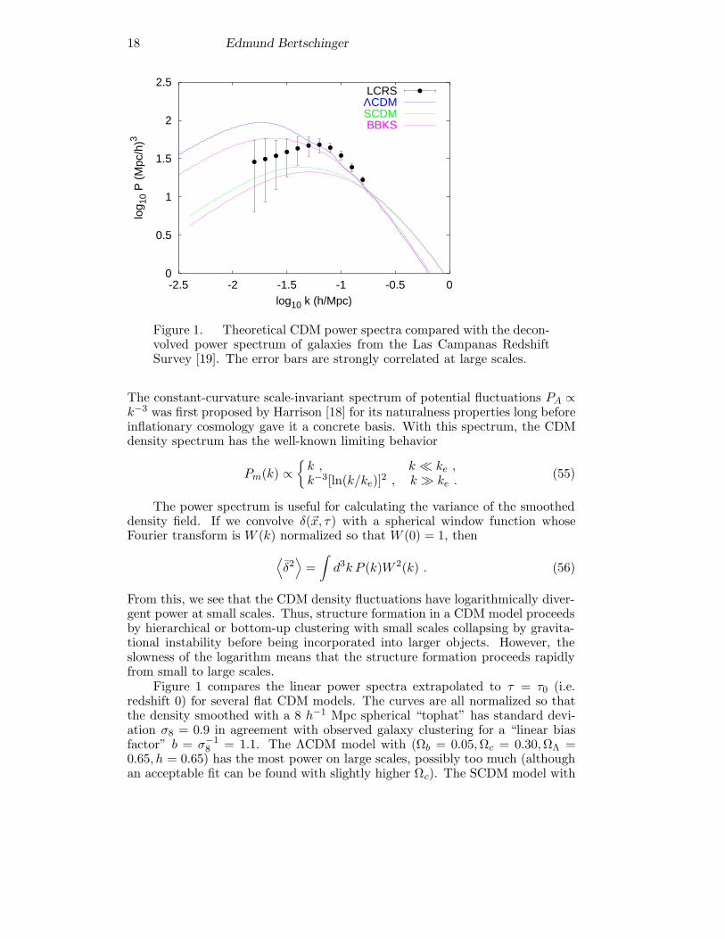
Figure 1. Theoretical CDM power spectra compared with the decon-volved power spectrum of galaxies from the Las Campanas RedshiftSurvey [19]. The error bars are strongly correlated at large scales.

The constant-curvature scale-invariant spectrum of potential fluctuations PA ∝k−3 was first proposed by Harrison [18] for its naturalness properties long beforeinflationary cosmology gave it a concrete basis. With this spectrum, the CDMdensity spectrum has the well-known limiting behavior

Pm(k) ∝k , k ke ,k−3[ln(k/ke)]2 , k ke .

(55)

The power spectrum is useful for calculating the variance of the smootheddensity field. If we convolve δ(~x, τ) with a spherical window function whoseFourier transform is W (k) normalized so that W (0) = 1, then

⟨δ2⟩

=∫d3k P (k)W 2(k) . (56)

From this, we see that the CDM density fluctuations have logarithmically diver-gent power at small scales. Thus, structure formation in a CDM model proceedsby hierarchical or bottom-up clustering with small scales collapsing by gravita-tional instability before being incorporated into larger objects. However, theslowness of the logarithm means that the structure formation proceeds rapidlyfrom small to large scales.

Figure 1 compares the linear power spectra extrapolated to τ = τ0 (i.e.redshift 0) for several flat CDM models. The curves are all normalized so thatthe density smoothed with a 8 h−1 Mpc spherical “tophat” has standard devi-ation σ8 = 0.9 in agreement with observed galaxy clustering for a “linear biasfactor” b = σ−1

8 = 1.1. The ΛCDM model with (Ωb = 0.05,Ωc = 0.30,ΩΛ =0.65, h = 0.65) has the most power on large scales, possibly too much (althoughan acceptable fit can be found with slightly higher Ωc). The SCDM model with


(Ωb = 0.05,Ωc = 0.95, h = 0.50) has too little power on large scales. Whencombined with the CMB anisotropy, this provides a strong argument for darkenergy (e.g. a cosmological constant) [20].

The curves labeled “BBKS” show the linear power spectra for the ΛCDMand SCDM models in the limit Ωb = 0 (with Ωc = 0.35 and 1.0 for the two mod-els, respectively). They are obtained from the fitting formula given by equation(G3) of [17] and agree well with full calculations using the COSMICS code [21],which was used for the other curves in Figure 1. Baryons reduce the amount ofsmall-scale power relative to scales k < ke because they cannot experience grav-itational instability on scales smaller than the photon-baryon Jeans length untilafter recombination. The oscillations in the ΛCDM power spectrum are alsodue to baryons and are similar to the cosine integral contributions to δc(k) inequation (51). They arise from the acoustic oscillations of the baryons betweenτe and τrec. When the power spectra are normalized at small scales (as theyeffectively are with σ8), increasing the baryon fraction increases the amount oflarge-scale power.

Aside from the baryon effect, the main parameter affecting the CDM spec-trum (and the only one in the BBKS formula) is ke. As may be checked usingequation (50), the peak of the CDM power spectrum is closely equal to ke.Measurements of galaxy clustering actually constrain ke/h = 0.1Γ Mpc−1 whereΓ ≡ Ωmh is a commonly used parameter. However, as Figure 1 shows, a sec-ond parameter, the baryon fraction Ωb/Ωm, also significantly affects the CDMspectrum.

5.2. Evolution of Large Scale Structure

The results given above concerned the shape of the CDM power spectrum, whichis frozen in after the universe becomes matter-dominated. However, the ampli-tude grows as a(τ) as assumed in equation (53) only if Ωm = 1. While this is agood approximation soon after recombination, it breaks down at small redshiftwhen Ωm < 1 today. In this case we must include dark energy, curvature, andany other important contributor to the expansion rate of the universe.

The evolution of CDM density fluctuations for τ τe is given by equations(14) and (20) ignoring the radiation terms. On subhorizon scales for φ2 δ2m 1 we have

∂2τ δm +

a

a∂τ δm = 4πGa2ρmδm =

32ΩmH

20

δma. (57)

Because the coefficients are spatially homogeneous, the time and space depen-dences of the solution factor: δm(~x, τ) = δ+(~x )D+(τ) + δ−(~x )D−(τ). ForΩm > 0, D+ grows with time and D− decays. For Ωm = 1 the growing solutionis D+ = a. For Ωm < 1 the solutions depend on the curvature K (sometimesexpressed as ΩK = −K/H2

0 ) and on the equation of state of the dark energy.See Peebles [22] and Peacock [15] for examples.

Peculiar velocities offer another probe of large-scale structure that is sensi-tive directly to all matter, dark or luminous. The divergence of peculiar velocity~v = d~x/dτ depends on the growth rate of density fluctuations:

θm ≡ ~∇ · ~vm = −∂τδm = −(d lnD+

d ln a

)aHδm for δ2m 1 . (58)


Measurements of galaxy velocities actually give ~v/aH, so that the ratio of ve-locity divergence to density fluctuation gives the logarithmic growth rate ofdensity fluctuations. An empirical fit to a range of models gives d lnD+/d ln a =f(Ωm) ≈ Ω0.6. In practice, the galaxy number density may be a biased tracerof the total matter density, conventionally parameterized by the bias factor b:δgalaxies = bδm. Comparing galaxy clustering and velocities then allows determi-nation of Ω0.6

m /b.

5.3. Numerical Simulation Methods

Linear theory breaks down once dark matter clumps become significantly denserthan the cosmic mean. Once this happens, full numerical simulations are neededto accurately follow the nonlinear dynamics of structure formation. Moreover,radiative processes, star formation, and supernova feedback have a strong effecton the baryonic component once galaxies begin forming. Although these pro-cesses can only be included in simulations in a phenomenological way, numericalsimulations are still the best way to advance our theoretical understanding ofstructure formation deep into the nonlinear regime.

Here we present only a brief synopsis of numerical simulation methods. Fora comprehensive review of both the methods and their applications see [23].

Particle methods are used for representing the dark matter. The phasespace of dark matter is represented by a sample of particles evolving under theirmutual gravitational field:

d~xi

dτ= ~vi ,

d~vi

dτ= − a

a~vi − ~∇φ , ∇2φ = 4πGa2

∑

j

mjδD(~x− ~xi)− ρm(τ)

(59)where δD is the Dirac delta function. In practice, the particles are spread overa softening distance to avoid unphysical two-body relaxation due to large-anglescattering. (A simulation may use particles of mass 109 M, leading to un-physical tight binaries if the forces are not softened.) The art of dark mattersimulation is mainly in calculating forces much faster than O(N2) for a soften-ing distance several orders of magnitude smaller than the simulation volume. Avariety of algorithms and codes are available; see [23] for details.

The initial conditions for dark matter positions and velocities are given fromlinear theory by the Zel’dovich approximation [7], which relates the comovingposition to its initial value ~q, a Lagrangian variable (i.e. one that labels eachparticle):

~x(~q, τ) = ~q +D+(τ)~ψ(~q ) , ~∇q · ~ψ = −δm . (60)

The initial density fluctuation field δm(~x, τ) is obtained as a sample of a gaussianrandom field with appropriate power spectrum.

Baryon physics is added by numerical integration of the fluid equations (17)and (18) with the addition of heating and cooling, ionization, etc. There aretwo classes of methods in widespread use in cosmology: smoothed-particle hy-drodynamics (SPH) and grid-based methods. SPH is an extension of the N-bodydynamics of equations (59) to include pressure forces and thermodynamics. Ithas the advantage of concentrating the spatial resolution and computational


effort where the baryons are densest, with the drawback of relatively large nu-merical viscosity and diffusivity owing to the particle discreteness. Grid-basedmethods use finite-difference techniques to approximate the fluid equations ona (usually) regular lattice. High accuracy methods developed for aerodynamicand other applications provide excellent resolution of shock waves, but with aresolution limited by the grid. Adaptive mesh refinement techniques are nowbeing used to refine the resolution where needed, resulting in the ability to followstructure formation to much higher densities than previously possible [24].

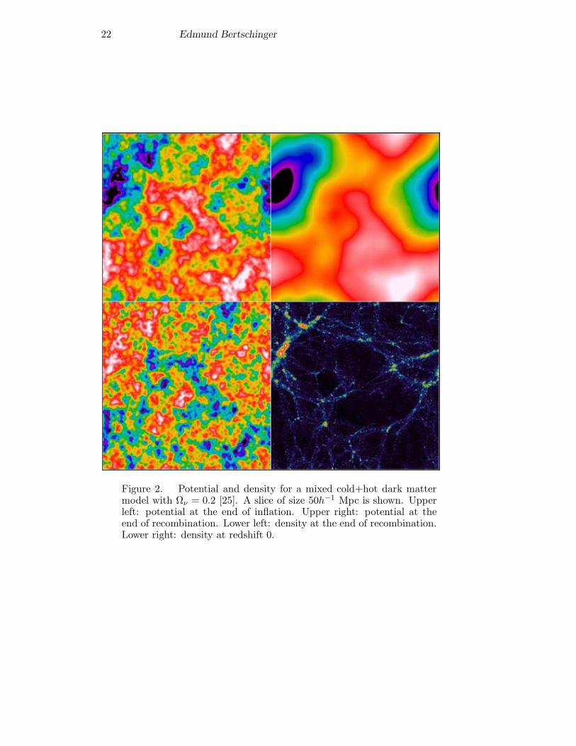
We conclude this introduction to numerical simulation methods with a mo-saic of gravitational potential and dark matter density from a high-resolutionsimulation of the mixed cold+hot dark matter model. Figure 2 shows the lineartheory and nonlinear simulation results. On the scales shown, ΛCDM would bealmost indistinguishable.

The gravitational potential shown in Figure 2 is a statistical fractal at theend of inflation, viz. a gaussian random field with power spectrum PA ∝ k−3.During the radiation era, acoustic damping smooths the potential on scalessmaller than k−1

e . Because the density fluctuations are related to the potentialby two spatial derivatives, the corresponding linear density field is dominated byhigh spatial frequency components. Indeed, if not for the smoothing imposed byfinite spatial resolution, the variance of density fluctuations would be logarith-mically divergent. It is instructive to compare the post-recombination densitywith the inflationary potential. The density is almost proportional to the po-tential but with opposite sign. This is because the density/potential transferfunction (52) varies only logarithmically on small scales.

The nonlinear evolution of the density field causes the mass to clusterstrongly into wispy filaments and dense clumps; most of the volume has lowdensity. The intermittency of structure is a sign of strong deviations from gaus-sian statistics.

5.4. Press-Schechter Theory

Numerical simulations show that most of the mass falls into dense self-gravitatingclumps. As a crude approximation, let us suppose that the mass profile of everyclump is spherically symmetric. In this case every gravitationally bound shellwill eventually fall into the center of the clump, at a time that is dependenton the enclosed mass and energy of the shell. For linear growing mode initialconditions, collapse occurs when linear theory would predict that the meandensity contrast interior to the shell is δc = 1.686 [15]. Thus, in the sphericalmodel, the distribution of clump masses is simply dependent on the statistics ofthe smoothed linear density field.

Press and Schechter [26] devised an elegant method for computing the massdistribution of gravitationally bound clumps using the simple spherical model.Their procedure is first to smooth the linear density field by convolution with aspherical “tophat” of radius R enclosing mean mass M(R) = (4π/3)ρmR

3:

δm(~x ) =∫d3x′WR(|~x− ~x ′|)δm(~x ′) , WR(r) =

34πR3

1, r < R ,0, r > R .

(61)

According to the Press-Schechter ansatz, the regions of the initial density fieldwith δ > δc = 1.686 at time τ have collapsed into objects of mass at least M . It


Figure 2. Potential and density for a mixed cold+hot dark mattermodel with Ων = 0.2 [25]. A slice of size 50h−1 Mpc is shown. Upperleft: potential at the end of inflation. Upper right: potential at theend of recombination. Lower left: density at the end of recombination.Lower right: density at redshift 0.


is easy to see that this would be true for a single spherical density perturbation;the genius is applying this to the entire density field.

Under this model, the fraction of mass in the universe contained in clumpsmore massive than M is

1ρm

∫ ∞

MdM M

dn

dM= P (δ > δc|M, τ) . (62)

On the left-hand side, (dn/dM)dM is the number density of clumps of mass in(M,M + dM); the integral gives the total mass density in clumps more massivethan M . Dividing by ρ gives the mass fraction. On the right-hand side, P (δ >δc|M, τ) is the probability that a randomly chosen point in the linear densityfield has δ > δc at time τ , where M defines the smoothing scale of δ. For agaussian random field of density fluctuations, this probability is simply

P =12erfc

(δc

σ√

2

)(63)

where erfc is the complementary error function and σ2 = σ2(M, t) = 〈δ2〉 is thevariance of the smoothed density. From equation (62) we can deduce dn/dM bydifferentiating with respect to M .

Now, as M → 0, σ(M) grows without bound for CDM models with loga-rithmically diverging power on small scales, so that P (δ > δc|M = 0, τ) = 1

2 .Half of the mass initially is in overdense regions, half is in underdense regionsδ < 0 which in linear theory can never collapse. However, this is plainly unphys-ical, as simulations show that virtually all of the mass, including that in initiallyunderdense regions, accretes onto dense clumps. Thus, Press and Schechter sug-gested doubling dn/dM so that all of the mass resides in dense clumps. Thus,their formula for the mass distribution of clumps is

dn

dM=

2ρM

∂P

∂M. (64)

Although realistic gravitational collapse is far more complex than imaginedin this derivation, equation (64) gives surprisingly good agreement with clumpmasses measured in cosmological N-body simulations [27]. The Press-Schechtermodel and its generalizations have proved to be a very useful tool for comparingab initio theories (power spectrum and cosmological model) with observationsof galaxies and galaxy clusters.

6. Conclusions

These lecture notes have presented a few of the theoretical elements useful for un-derstanding the microwave background and structure formation. Cosmology israpidly changing with the advent of precision measurements of CMB anisotropy,with the observation of galaxies at z > 3, and with large new redshift surveys.Theoretical research has become more phenomenological, with a focus on pro-viding the framework for interpreting and analyzing the new data. Despitethis trend—or perhaps because of the high quality of new data—theoreticalcosmology still requires further development of the basic processes of structureformation. Either way, I hope that the material presented in these lectures willbe useful to cosmology graduate students.


Acknowledgments. I would like to thank Sergei Bashinsky for help withthe two-fluid solutions. I am grateful to the organizers, the other speakers, andthe students of the Cosmology 2000 summer school for the fruitful, stimulat-ing atmosphere in Lisbon. Special thanks are due to the organizers for theirwonderful hospitality. This work was supported by NSF grant AST-9803137.

References

[1] E. Bertschinger, in Cosmology and Large Scale Structure, proc. Les HouchesSummer School, Session LX, ed. R. Schaeffer, J. Silk, M. Spiro, and J.Zinn-Justin, Elsevier Science, Amsterdam (1996) 273.

[2] C.-P. Ma and E. Bertschinger, ApJ 455 (1995) 7.

[3] E. M. Lifshitz, J. Phys. USSR 10 (1946) 116.

[4] C.W. Misner, K.S. Thorne, and J.A. Wheeler, Gravitation, Freeman, SanFrancisco (1973).

[5] Gravity Probe B website, http://einstein.stanford.edu/.

[6] J.M. Bardeen, Phys.Rev.D 22 (1980) 1882.

[7] Ya.B. Zel’dovich, A&A 5 (1970) 84.

[8] P.J.E. Peebles and R.H. Dicke, ApJ 154 (1968) 891.

[9] U. Seljak and M. Zaldarriaga, ApJ 469 (1996) 437.

[10] W. Hu, U. Seljak, M. White, and M. Zaldarriaga, Phys.Rev.D 57 (1998)3290.

[11] P. Schneider, J. Ehlers, and E.E. Falco, Gravitational Lenses, Springer-Verlag, Berlin (1992).

[12] U. Seljak, ApJ 463 (1996) 1.

[13] P.J.E. Peebles and J.T. Yu, ApJ 162 (1970) 815.

[14] R.K. Sachs and A.M. Wolfe, ApJ 147 (1967) 73.

[15] J.A. Peacock, Cosmological Physics, Cambridge Univ. Press (1999).

[16] S. Bashinsky and E. Bertschinger, astro-ph/0012153.

[17] J.M. Bardeen, J.R. Bond, N. Kaiser, and A.S. Szalay, ApJ 304 (1986) 15.

[18] E.R. Harrison, Phys.Rev.D 1 (1970) 2726.

[19] H. Lin et al., ApJ 471 (1996) 617.

[20] M. Tegmark, M. Zaldarriaga, and A.J.S. Hamilton, astro-ph/0008167.

[21] E. Bertschinger, astro-ph/9506070 and http://arcturus.mit.edu/cosmics/.


[22] P.J.E. Peebles, The Large-Scale Structure of the Universe, Princeton Univ.Press (1980).

[23] E. Bertschinger, ARA&A 36 (1998) 599.

[24] T. Abel, G.L. Bryan, and M.L. Norman, ApJ 540 (2000) 39.

[25] C.-P. Ma and E. Bertschinger, ApJ 434 (1994) L5.

[26] W.H. Press and P. Schechter, ApJ 187 (1974) 425.

[27] S. Cole and C. Lacey, MNRAS 281 (1996) 716.

Documents

Cosmological Perturbation Theory and Structure Formationcds.cern.ch/record/484698/files/0101009.pdf · Cosmological Perturbation Theory and Structure ... treatment of large scale