VOLUME65, NUMBER3 P H Y S I C A L R E V I E W L E T T E R S 16JULY 1990

Cosmic Gravitational-Wave Background: Limits from Millisecond Pulsar Timing

D. R. Stinebring, M. F. Ryba, and J. H. Taylor Joseph Henry Laboratories and Physics Department, Princeton University, Princeton, New Jersey 08544

R. W. Romani Institute for Advanced Study, Princeton, New Jersey 08540

(Received 26 March 1990)

We use seven years of millisecond pulsar-timing data to derive rigorous upper bounds on a cosmic gravitational-wave background. The energy density per logarithmic frequency interval near /—0.14 yr"1 must be < 9 x l 0 ~ x (68% confidence), or < 4 x l 0 ~ 7 (95% confidence), of the density required to close the Universe. We detect a red-noise signal in the residuals for one pulsar. Its spectrum appears flatter than the f~* power law expected for a gravity-wave background; likely noise sources include changes in the interstellar medium and pulsar rotational instabilities.

PACS numbers: 04.80,+z, 95.30.Sf, 97.60.Gb, 98.80.Es

The use of pulsar-timing data to detect or place limits on low-frequency gravitational waves was first suggested twelve years ago1 ,2 and put into practice a few years later.3,4 The underlying principle is the same as that of laboratory gravitational-wave detectors that use laser in-terferometry to measure the separations of suspended masses. The Earth and a distant pulsar (PSR) are treat­ed as free masses whose positions respond to changes in the local spacetime metric. Passing gravitational waves perturb the metric, and produce fluctuations in the mea­sured pulse arrival times. If pulse time-of-arrival (TOA) observations have uncertainties St and span an interval 7\ the experiment will be sensitive to waves with dimen-sionless amplitudes of order St/T and frequencies down to / — \/T. A thorough discussion of the technique, in­cluding many practical caveats concerning data analysis, may be found in Ref. 5.

We began making timing observations of PSRs 19374-21 and 1855+09 at the Arecibo Observatory soon after their discoveries.67 Results of the project have been summarized at several stages previously;8"10 experi­mental details may be found in these references and in a more extensive work now in preparation. Observations have been made at approximately biweekly intervals, at frequencies near 1408 and 2380 MHz. PSR 1855+09 is observed only at the lower frequency; by the end of 1989 its accumulated data set contained 66 TOAs spanning 3.9 yr. For PSR 1937+21 we have obtained 169 TOAs over 7.1 yr at 1408 MHz, and 102 over 5.2 yr at 2380 MHz.

On a particular observing day, measurements typically consist of fifteen 2-min integrations for each pulsar at each scheduled frequency. The detected signals are syn­chronously averaged, using an ephemeris prepared in ad­vance. Integrated profiles are tagged with their starting times according to the observatory master clock, and recorded digitally. Phases of the integrated wave forms are determined by means of an optimized least-squares

technique performed in the Fourier-transform do­main.1 1 1 2 The phases are multiplied by the pulsar period and added to the start times of the integrations, yielding topocentric TOAs. For the purposes of this pa­per, we have reduced the TOAs to a single daily "normal point" for each pulsar at each observing frequency.

The normal-point TOAs are corrected for offsets of the observatory clock relative to UTC (NIST) , using the global positioning system common-view technique for time transfer. A further correction yields TOAs accord­ing to TT (BIPM90), a retrospective weighted-average time scale intended to be the most stable atomic time reference. These values are relativistically transformed to the solar-system barycenter, using the Jet Propulsion Laboratory DE200 ephemeris to determine the location of the geocenter, tables published by the International Earth Rotation Service to specify the rotational phase of the Earth, and an analytic expression13 for the relativis­t s correction from proper terrestrial time to barycentric dynamical time. Final transformations account for in­terstellar dispersion and binary orbital motion,14 if any, yielding proper times in the pulsar frame.

Starting with the best available parameters for each pulsar, we compute the pulsar rotational phase corre­sponding to each TOA. The residuals, or differences be­tween observed and computed phases, can be used to determine refinements to the pulsar parameters as well as to investigate unmodeled sources of timing noise. For the present analysis we determined the astrometric pa­rameters, dispersion measures, and orbital elements from subsets of data short enough that the residuals were clearly dominated by uncorrected, "white-noise" mea­surement errors. On the basis of these parameters, a final set of residuals was determined for each of three data sets. These are expressed in time units and plotted in Fig. 1.

The residuals for PSR 1855+09 are dominated by white-noise measurement errors having typical ampli-

© 1990 The American Physical Society 285

VOLUME 65, NUMBER 3 PHYSICAL REVIEW LETTERS 16 JULY 1990

J ' 1 ' 1 ' 1 (b)

. -

w •

"1 1 1 , 1 1 1

1 1

••

1 1

1 1 • •

mm.* *

•

1 1

1 1

•*..>, • •

I 1

1 L|

-

s.: , r

J

~\

1 i ' 1 (c)

1 1 1 1

1 1 ' 1 •

• • • • • • • f

m • 1 1 1 1

1 1 ' J ' Lj • —

• 1 • • -A

• • • \

:

i i i i i r 83 84 85 86 87

Year 88 89 90

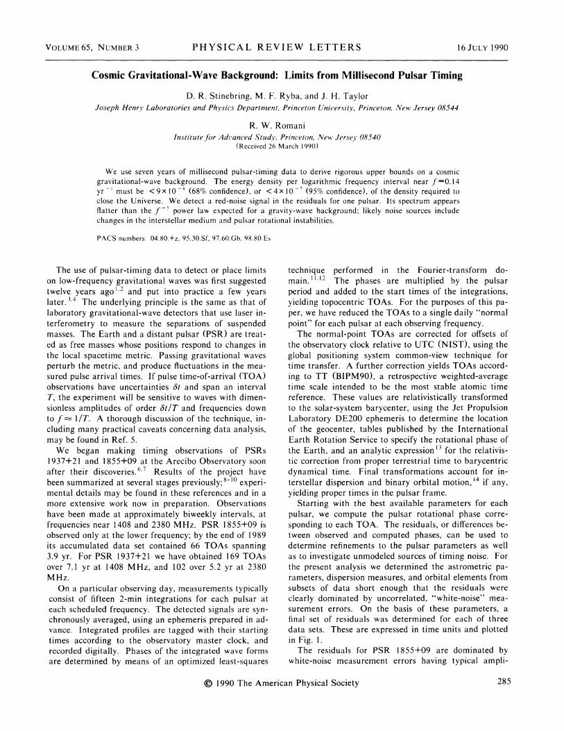
FIG. 1. Pulsar-timing residuals for three data sets: (a) PSR 1937+21 at 1408 MHz, (b) PSR 1937+21 at 2380 MHz, and (c) PSR 1855+09 at 1408 MHz. The same period and period derivative were assumed in calculating the residuals in (a) and (b); differences in the overlapping region are dominated by the small, smoothly varying adjustments for changes in dispersion measure (Ref. 10) that have been applied to (b) but not (a).

tude 1.7 j/s. The two sets of data for PSR 1937+21, however, contain both a white-noise component ( — 0.4 /is over most of the 7.1-yr data span) and a steep-spectrum "red" component. The red noise is qualitative­ly similar to the intrinsic timing noise observed in some young pulsars.15 However, at the level of several fis of accumulated fluctuations, there may be other significant noise sources as well. The most plausible candidates516

should have approximately power-law spectra, P(f) = Pof~a, with indices a = 0 (white noise), 2-4 (clock in­stabilities, ephemeris errors, interstellar propagation effects, pulsar rotational instabilities), and 5 (cosmic gravitational-wave background). Spectral analysis of the residuals should help to discriminate among these possi­bilities.

Estimation of the spectral content of red-noise random processes has received extensive treatment in the astro-physical literature15 ,7~19 and also in the literature of time-keeping metrology.20 Traditional methods of spec­tral analysis based on discrete Fourier transforms fail in the presence of very red noise because of severe spectral leakage. A method using orthonormal polynomials as

basis functions provides nearly optimal bandpasses for red power-law spectra, and is computationally con­venient for irregularly sampled data. ,9

We have used a procedure that begins with a sequence of timing residuals r(t,), / = 1, . . . ,7V. By means of a Gram-Schmidt procedure, we obtain the coefficients of a set of polynomials of order j =0, . . . ,3, orthonormal over this set of /,'s so that

^ (1)

A linear least-squares fit of these basis functions to the residuals yields the values of constants C7 that minimize the sum

x — 7 L y = 0

(2)

The first three C/s are fully covariant with the values adopted for the rotational phase, period, and period derivative of the pulsar; any information on the noise in their passband is absorbed by the spin parameters. The square of C) provides an estimate S\ of the spectral power density at the lowest frequencies to which the ex­periment is sensitive, f ~ \/T.

The data set is then divided into m =2, 4, and 8 ap­proximately equal-time sequences, and the above pro­cedure is repeated. Each subdivision results in m new C3's and a spectral density estimate Sm=(C]) that responds to fluctuation power an octave higher in fre­quency than Sm-\. We do not proceed beyond m =8 (or beyond m =4 for PSR 1855+09) because further subdi­vision would leave insufficient data in the subsequences. Moreover, in the present data sets, frequencies above those measured for m = 8 are dominated by the white-noise measurement errors, and such noise is not best ana­lyzed with orthonormal polynomials.

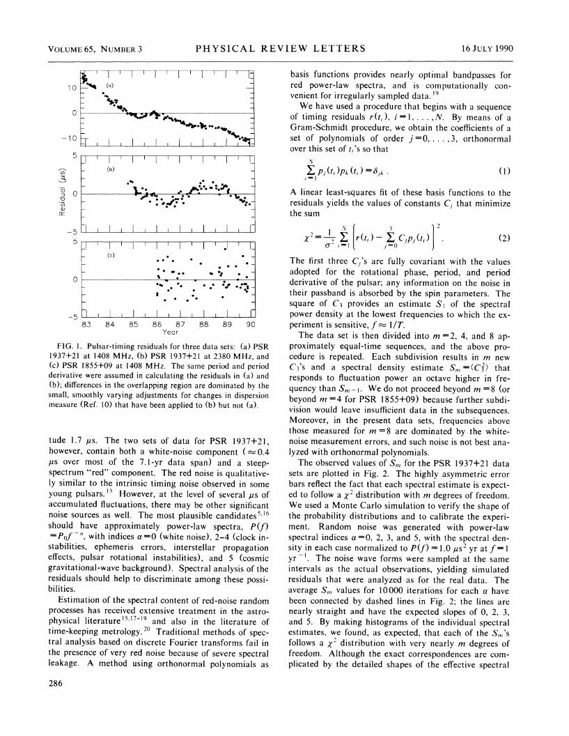
The observed values of Sm for the PSR 1937+21 data sets are plotted in Fig. 2. The highly asymmetric error bars reflect the fact that each spectral estimate is expect­ed to follow a x1 distribution with m degrees of freedom. We used a Monte Carlo simulation to verify the shape of the probability distributions and to calibrate the experi­ment. Random noise was generated with power-law spectral indices a = 0 , 2, 3, and 5, with the spectral den­sity in each case normalized to P(f) = 1.0 jus2 yr a t / = l y r - 1 . The noise wave forms were sampled at the same intervals as the actual observations, yielding simulated residuals that were analyzed as for the real data. The average Sm values for 10000 iterations for each a have been connected by dashed lines in Fig. 2; the lines are nearly straight and have the expected slopes of 0, 2, 3, and 5. By making histograms of the individual spectral estimates, we found, as expected, that each of the S„,'s follows a x2 distribution with very nearly m degrees of freedom. Although the exact correspondences are com­plicated by the detailed shapes of the effective spectral

286

V O L U M E 65, N U M B E R 3 P H Y S I C A L R E V I E W L E T T E R S 16 J U L Y 1990

-

_

—

1 1 i

\ \ \ \ -

1 l 1 1 2 4 8 1 2 4 8

Frequency index, m Frequency index, m

FIG. 2. Circles with error bars represent spectral measure­ments of residuals for the data sets of Figs. 1 (a) (left) and 1(b) (right). Dashed lines correspond to the mean spectral densities obtained for simulated power-law noise over the same time intervals, with spectral indices 0, 2, 3, and 5, and spectral density />(/)=* 1.0 ^s2yr at f=\ y r - 1 . The index m can be converted approximately to cycles per year by dividing by the data spans, 7 — 7.1 yr and 7=5.2 yr, respectively, for the two data sets. The steepest dashed lines correspond to the expected gravitational-wave background signal if Cl^h2 had the unlikely large value of 7.5 x 10 ~ \

passbands, it is possible to relabel the axes of Fig. 2 so that they correspond approximately to spectral density P(f). The appropriate scalings are such that f~m/T, and P (/)=*{ jjs2yv where the simulated spectra for a = 2, 3, and 5 almost intersect, namely, at / « 1 y r - 1 . The simulated spectrum for a = 0 lies considerably above the intersection of the others, because for white noise the 5,,,'s have poor spectral cutoffs on their high-frequency sides.

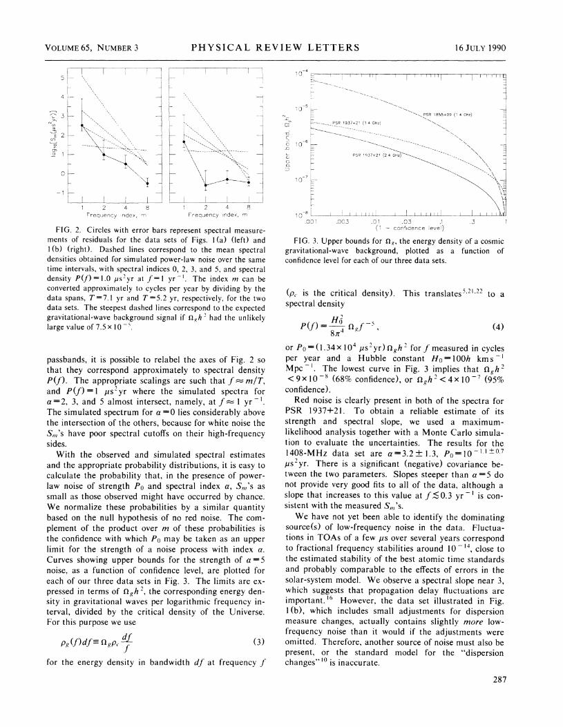
With the observed and simulated spectral estimates and the appropriate probability distributions, it is easy to calculate the probability that, in the presence of power-law noise of strength Po and spectral index a, S„,'s as small as those observed might have occurred by chance. We normalize these probabilities by a similar quantity based on the null hypothesis of no red noise. The com­plement of the product over m of these probabilities is the confidence with which P§ may be taken as an upper limit for the strength of a noise process with index a. Curves showing upper bounds for the strength of a = 5 noise, as a function of confidence level, are plotted for each of our three data sets in Fig. 3. The limits are ex­pressed in terms of flgh

2, the corresponding energy den­sity in gravitational waves per logarithmic frequency in­terval, divided by the critical density of the Universe. For this purpose we use

Pg(f)df=agPr4jr (3)

for the energy density in bandwidth df at frequency /

i y ^ | , | • i r-]-r| I I r i i i i i I i r~i i i i i H

" ^ \ PSR 1855+09 (1 4 Ghz)

f SR 1937 + 21 (1 4 GHz) " " \

(1 - confidence level)

FIG. 3. Upper bounds for fi?, the energy density of a cosmic gravitational-wave background, plotted as a function of confidence level for each of our three data sets.

(pc is the critical density). This translates5 ,21 ,22 to a spectral density

/ > ( / ) = - ^ n , / ~ \ (4) on

or Po = (1.34x 104 fis2yr)Clgh2 for / measured in cycles

per year and a Hubble constant / /o = 100/z k m s " 1

M p c - 1 . The lowest curve in Fig. 3 implies that flgh2

< 9 x l 0 " 8 (68% confidence), or n ^ 2 < 4 x l 0 " 7 (95% confidence).

Red noise is clearly present in both of the spectra for PSR 1937+21. To obtain a reliable estimate of its strength and spectral slope, we used a maximum-likelihood analysis together with a Monte Carlo simula­tion to evaluate the uncertainties. The results for the 1408-MHz data set are a = 3 . 2 ± 1 . 3 , / > o « 1 0 ~ n ± 0 - 7

/is2yr. There is a significant (negative) covariance be­tween the two parameters. Slopes steeper than a = 5 do not provide very good fits to all of the data, although a slope that increases to this value at / ; S 0 . 3 yr _ 1 is con­sistent with the measured Sm ' s .

We have not yet been able to identify the dominating source (s) of low-frequency noise in the data. Fluctua­tions in TOAs of a few ps over several years correspond to fractional frequency stabilities around 10 ~14, close to the estimated stability of the best atomic time standards and probably comparable to the effects of errors in the solar-system model. We observe a spectral slope near 3, which suggests that propagation delay fluctuations are important.16 However, the data set illustrated in Fig. 1(b), which includes small adjustments for dispersion measure changes, actually contains slightly more low-frequency noise than it would if the adjustments were omitted. Therefore, another source of noise must also be present, or the standard model for the "dispersion changes" l 0 is inaccurate.

287

VOLUME65, NUMBER3 PHYSICAL REVIEW LETTERS 16JULY 1990

The prospects for obtaining better discrimination among possible sources of low-frequency noise appear promising. Clock errors will affect all pulsars equally; if this source of fluctuating residuals is significant, it should become visible in the PSR 1855+09 data within another year or so. Since these two pulsars are separated by only 16° in the sky, ephemeris errors will also affect them similarly, but pulsars in other directions would show different ephemeris effects. Intrinsic timing noise will of course be uncorrelated in different pulsars, as will inter­stellar propagation changes. In principle, it is possible to carry out a global analysis of data from these pulsars and others, as comparable data sets are accumulated, looking for correlated fluctuations with the quadrupolar angular signature of gravitational waves.4,23 We plan to pursue this line of analysis.

Cosmologies using high-density seeds such as cosmic strings24 to initiate galaxy formation can produce sub­stantial amounts of relic gravitational radiation. Our present noise level, if due to gravitational waves with an f~5 spectrum, corresponds to O A 2;S 1 x 10 ~7. Despite recent progress, there remain large theoretical uncertain­ties in the evolutionary properties of cosmic strings. In the picture where long-lived loops (of size tf~10~2 of the horizon scale at formation) are responsible for ini­tiating galaxy formation, our present noise level gives an estimate of the string density per unit length of GJJ ;S2x 10_7(tf-2) ~ \ where the characteristic size of a loop is 10_2tf-2 and other parameters are fixed at reasonable values.25"27 Recent work suggests that a may be very small;27 in this case very conservative limits give Gfi ;S 102Hg 1 x 10 ~5. Detailed evolution of loop pop­ulations25,2 should give stronger bounds.

We thank D. C. Backer, M. M. Davis, L. A. Rawley, A. Vazquez, and J. M. Weisberg for essential contribu­tions to the project; D. Bennett, E. J. Groth, and N. Turok for helpful discussions; and the National Science Foundation (Grants No. AST88-17826 and No. PHY-86-29266), National Institute of Standards and Technol­ogy, and Corning Glass Works for financial support. Arecibo Observatory is operated by Cornell University, under contract with the NSF.

M. V. Sazhin, Astron. Zh. 55, 65 (1978) [Soviet Astron. 22,

36 (1978)]. 2S. Detweiler, Astrophys. J. 234, 1100 (1979). 3R. W. Romani and J. H. Taylor, Astrophys. J. Lett. 265,

L65 (1983). 4R. W. Hellings and G. S. Downs, Astrophys. J. Lett. 265,

L39 (1983). 5R. Blandford, R. Narayan, and R. W. Romani, J. Astro­

phys. Astron. 5, 369 (1984). 6D. C. Backer, S. R. Kulkarni, C. Heiles, M. M. Davis, and

W. M. Goss, Nature (London) 300, 615 (1982). 7D. J. Segelstein, L. A. Rawley, D. R. Stinebring, A. S.

Fruchter, and J. H. Taylor, Nature (London) 323, 714 (1986). 8M. M. Davis, J. H. Taylor, J. M. Weisberg, and D. C.

Backer, Nature (London) 315, 547 (1985). 9L. A. Rawley, J. H. Taylor, M. M. Davis, and D. W. Allan,

Science 238, 761 (1987). ,0L. A. Rawley, J. H. Taylor, and M. M. Davis, Astrophys. J.

326,947 (1988). ML. A. Rawley, Ph.D. thesis, Princeton University, 1986 (un­

published). ,2J. H. Taylor (to be published). 13L. Fairhead, P. Bretagnon, and J.-F. Lestrade, in The

Earth's Rotation and Reference Frames for Geodesy and Geo-dynamics, edited by A. K. Babcock and G. A. Wilkins (Kluwer, Dordrecht, 1988), p. 419.

14J. H. Taylor and J. M. Weisberg, Astrophys. J. 345, 434 (1989).

15J. M. Cordes and G. S. Downs, Astrophys. J. Suppl. 59, 343 (1985).

I6J. W. Armstrong, Nature (London) 307, 527 (1984). I7E. J. Groth, Astrophys. J. Suppl. 29, 443 (1975). I8J. Deeter and P. Boynton, Astrophys. J. 261, 337 (1982). I9J. Deeter, Astrophys. J. 281, 482 (1984). 20D. W. Allan, IEEE Trans. Ultrasonics, Ferroelectrics, and

Frequency Control 34, 647 (1987). 21B. Bertotti, B. J. Carr, and M. J. Rees, Mon. Not. Roy.

Astron. Soc. 203,945 (1983). 22C. J. Hogan and M. J. Rees, Nature (London) 311, 109

(1984). 23R. W. Romani, in Timing Neutron Stars, edited by H.

Ogelman and E. P. J. van den Heuvel (Kluwer, Dordrecht, 1989), p. 113.

24A. Vilenkin, Phys. Lett. 107B, 47 (1981). 25R. W. Romani, Phys. Lett. B 215, 477 (1988). 26N. Turok, Nucl. Phys. B242, 520 (1984). 27F. R. Bouchet and D. P. Bennett, Phys. Rev. D 41, 720

(1990). 28F. Acetta and L. Krauss, Nucl. Phys. B319, 747 (1989).

288