Correlated-Samples ANOVA

The Multivariate Approach

One-Way

Cross-Species-Fostering

• House mice onto house mice, prairie deer mice, or domestic Norway rats.

• After weaning, tested in apparatus with access to tunnels scented like clean pine shavings, house mouse, deer mouse, or rat.

• House mice and deer mice were descendants of recently wild-trapped mice.

• Reversed light cycle, red lighting

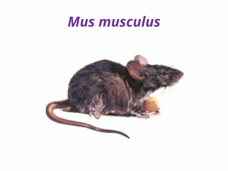
Mus musculus

Peromyscus maniculatus

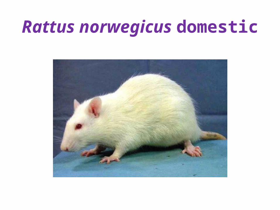
Rattus norwegicus domestic

Homo sapiens

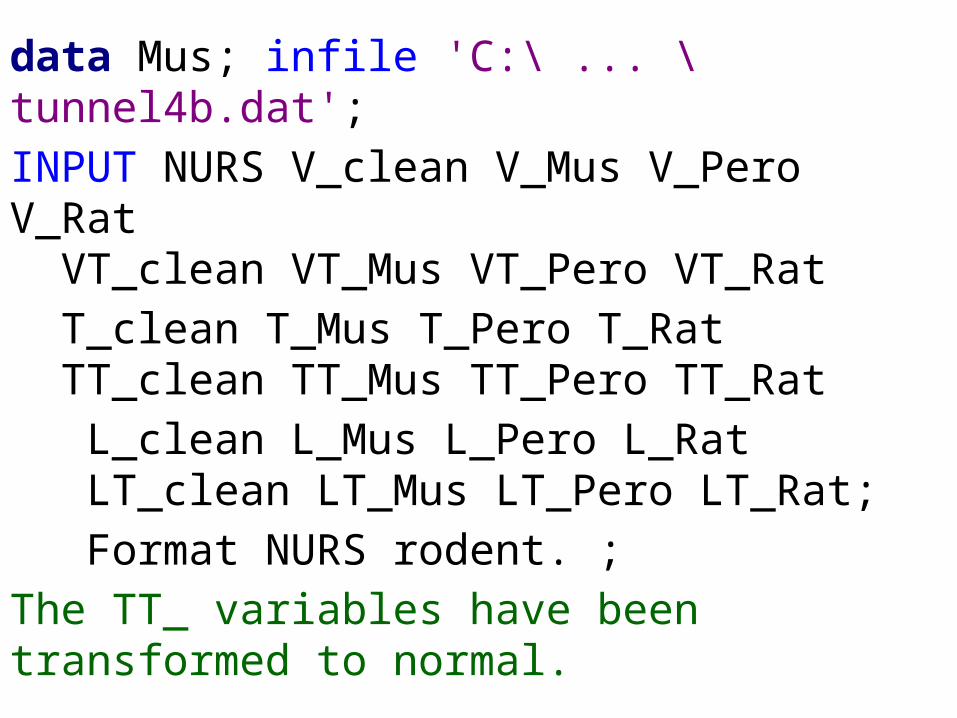
data Mus; infile 'C:\ ... \tunnel4b.dat';

INPUT NURS V_clean V_Mus V_Pero V_Rat VT_clean VT_Mus VT_Pero VT_Rat

T_clean T_Mus T_Pero T_Rat TT_clean TT_Mus TT_Pero TT_Rat

L_clean L_Mus L_Pero L_Rat LT_clean LT_Mus LT_Pero LT_Rat;

Format NURS rodent. ;

The TT_ variables have been transformed to normal.

The ANOVA

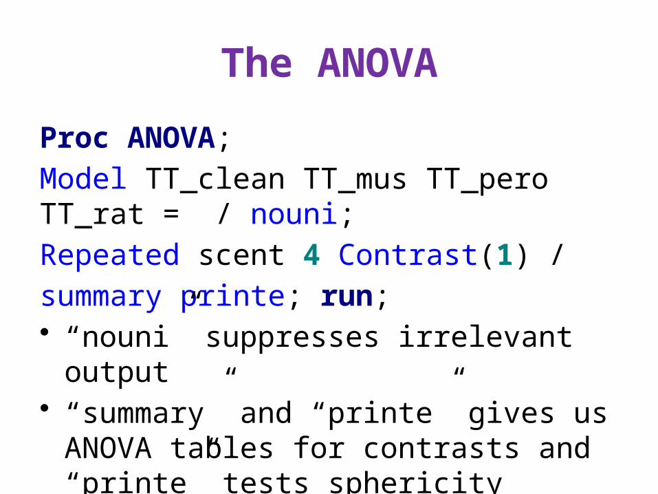
Proc ANOVA;

Model TT_clean TT_mus TT_pero TT_rat = / nouni;

Repeated scent 4 Contrast(1) /

summary printe; run;• “nouni” suppresses irrelevant output• “summary” and “printe” gives us ANOVA

tables for contrasts and “printe” tests sphericity

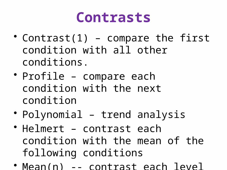
Contrasts• Contrast(1) – compare the first condition

with all other conditions.• Profile – compare each condition with the

next condition• Polynomial – trend analysis• Helmert – contrast each condition with the

mean of the following conditions• Mean(n) -- contrast each level (except the

nth) with the mean of all other levels.

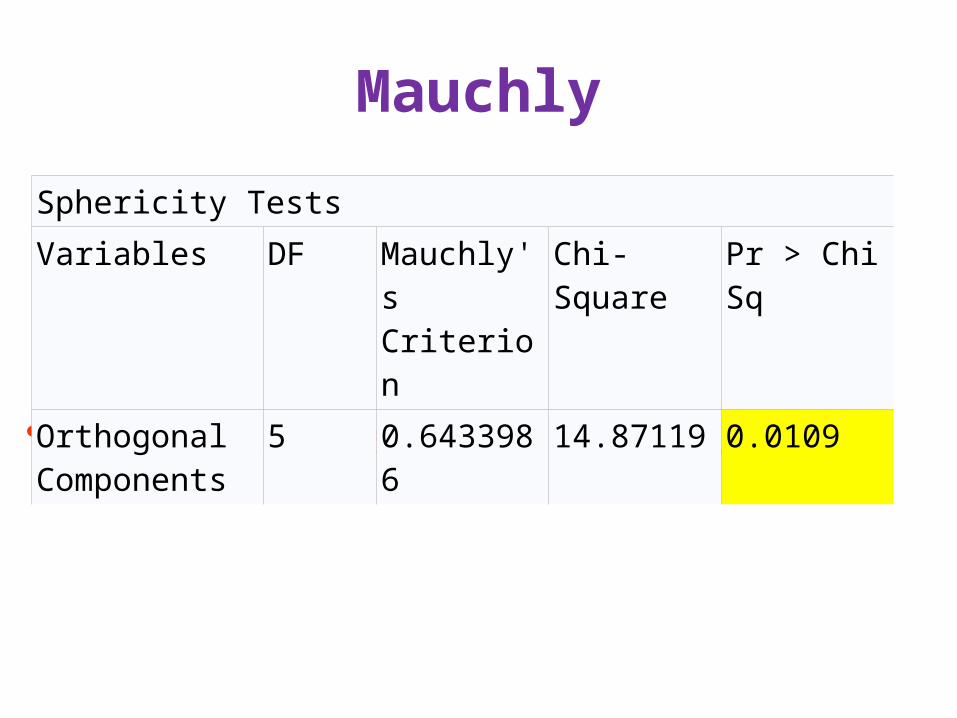
Mauchly

• Sphericity Assumption Violated

Sphericity TestsVariables DF Mauchly's

CriterionChi-Square Pr > ChiSq

Orthogonal Components

5 0.6433986 14.87119 0.0109

MANOVAMANOVA Test Criteria and Exact F Statistics for the Hypothesis of no scent Effect

Statistic Value F Value Num DF Den DF Pr > FWilks' Lambda

0.58343 7.85 3 33 0.0004

Pillai's Trace 0.41656 7.85 3 33 0.0004Hotelling-Lawley Trace

0.71398 7.85 3 33 0.0004

Roy's Greatest Root

0.71398 7.85 3 33 0.0004

Univariate ApproachSource DF Anova

SSMean Square

F Value

Pr > F Adj Pr > F

G - G H - F

scent 3 1467.267 489.089 7.01 0.0002 0.0009 0.0006

Error(scent) 105 7326.952 69.7804      

Greenhouse-Geisser Epsilon 0.7824Huynh-Feldt Epsilon 0.8422

• Both the G-G and the H-F are near or above .75, it is probably best to use the H-F

• df = 3(.8422), 105(.8422) = 2.53, 88.43

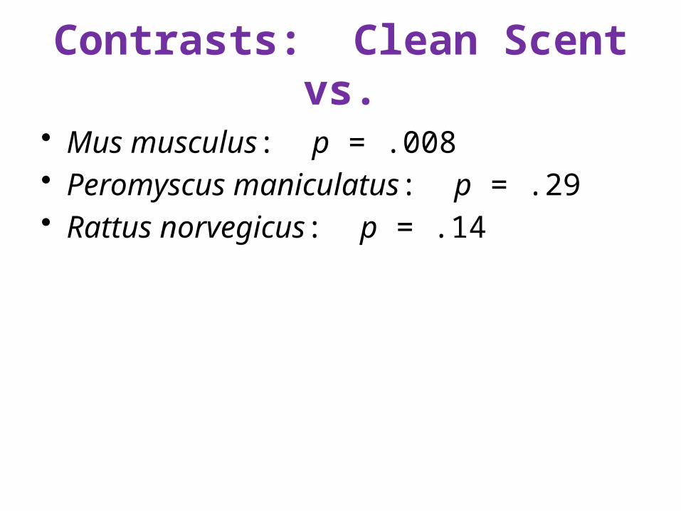
Contrasts: Clean Scent vs.

• Mus musculus: p = .008• Peromyscus maniculatus: p = .29• Rattus norvegicus: p = .14

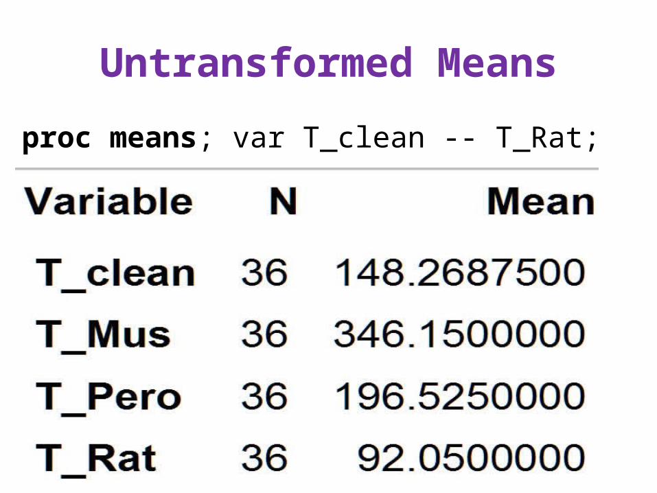
Untransformed Means

proc means; var T_clean -- T_Rat;

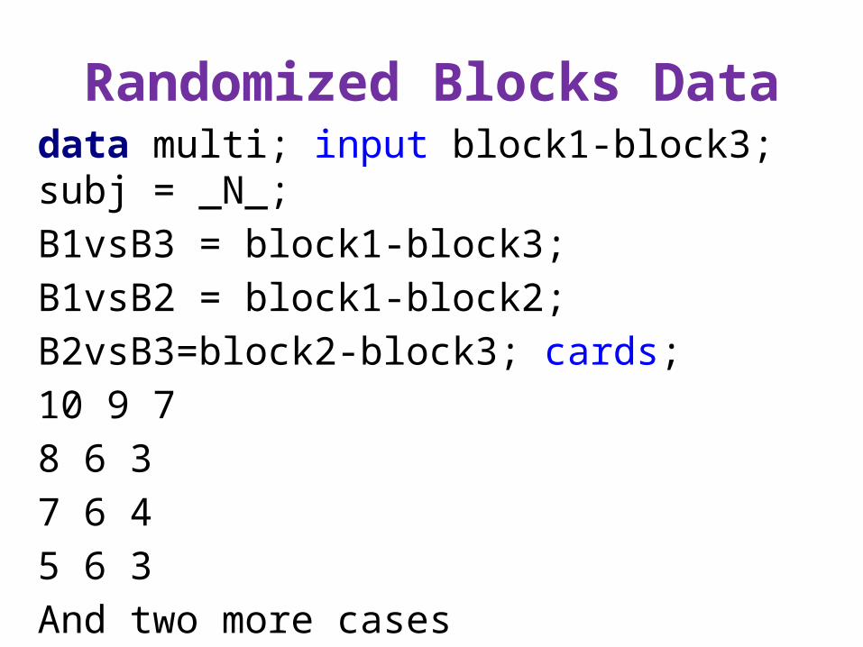
Randomized Blocks Datadata multi; input block1-block3; subj = _N_;

B1vsB3 = block1-block3;

B1vsB2 = block1-block2;

B2vsB3=block2-block3; cards;

10 9 7

8 6 3

7 6 4

5 6 3

And two more cases

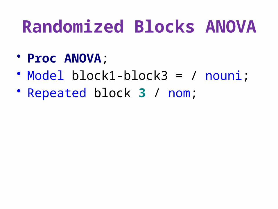
Randomized Blocks ANOVA

• Proc ANOVA;• Model block1-block3 = / nouni;• Repeated block 3 / nom;

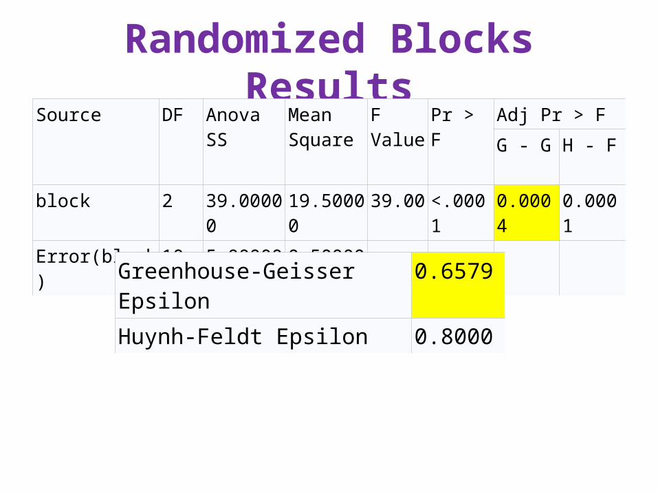
Randomized Blocks ResultsSource DF Anova

SSMean Square

F Value

Pr > F Adj Pr > F

G - G H - F

block 2 39.00000 19.50000 39.00 <.0001 0.0004 0.0001

Error(block) 10 5.000000 0.500000        

Greenhouse-Geisser Epsilon 0.6579Huynh-Feldt Epsilon 0.8000

Pairwise Comparisons

proc means t prt; var B1vsB3 B1vsB2 B2vsB3; run;

Want Pooled Error?

• The comparisons on previous slide use individual error terms.

• Get more power with pooled error.• First, unpack data from multivariate setup

to univariate setup.• Then use ANOVA with desired procedure

(LSD, Tukey, REGWQ, etc.)

Unpack the Data

data univ; set multi;

array b[3] block1-block3; do block = 1 to 3;

errors = b[block]; output; end; drop block1-block3;

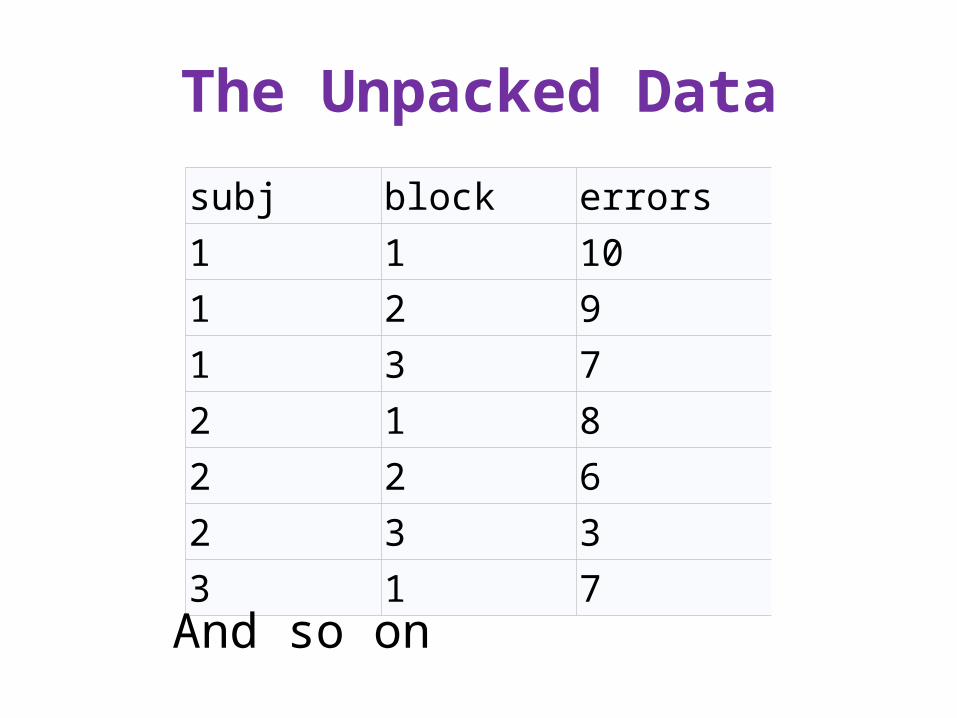
The Unpacked Data

subj block errors1 1 101 2 91 3 72 1 82 2 62 3 33 1 7

And so on

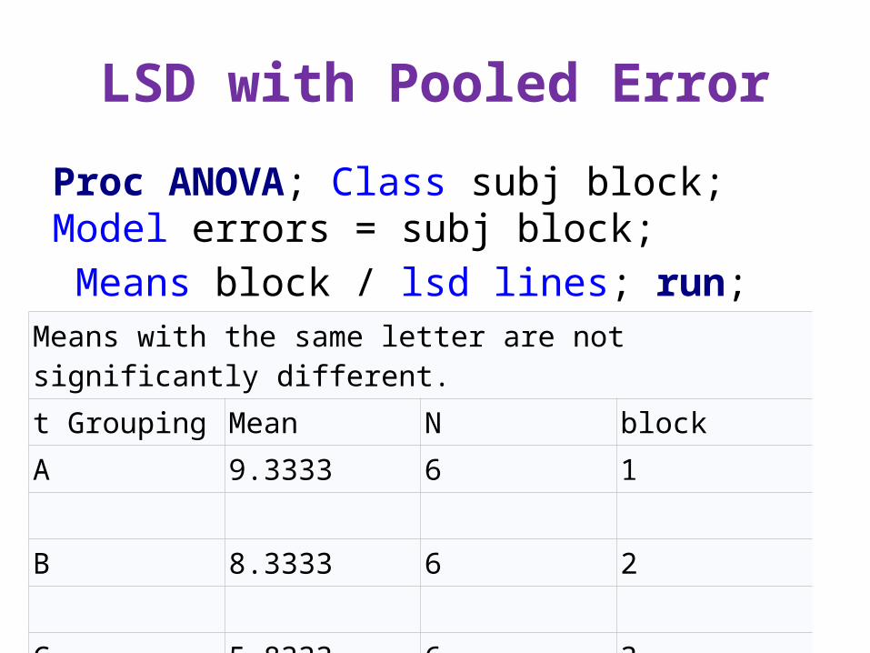
LSD with Pooled Error

Proc ANOVA; Class subj block; Model errors = subj block;

Means block / lsd lines; run;Means with the same letter are not significantly different.

t Grouping Mean N blockA 9.3333 6 1       B 8.3333 6 2       C 5.8333 6 3

SPSS

• Want to use SPSS instead of SAS?• See my document

The Multivariate Approach to the One-Way Repeated Measures ANOVA