Correlated Q-Learning Amy Greenwald, Keith Hall …cs.brown.edu/research/pubs/pdfs/2005/Greenwald-2005-CL.pdfCorrelated Q-Learning Amy Greenwald, Keith Hall and Martin Zinkevich Department

Correlated Q-Learning

Amy Greenwald, Keith Hall and Martin Zinkevich

Department of Computer Science

Brown University

Providence, Rhode Island 02912

CS-05-08

July 2005

Brown University Technical Report (2005) CS-05-08


Amy Greenwald [email protected]

Department of Computer ScienceBrown UniversityProvidence, RI 02912

Keith Hall keith [email protected]

Center for Language and Speech ProcessingJohns Hopkins UniversityBaltimore, MD 21201

Martin Zinkevich [email protected]

Department of Computer Science

Brown University

Providence, RI 02912

Abstract

Recently, there have been several attempts to design multiagent learning algorithms thatlearn equilibrium policies in general-sum Markov games, just as Q-learning learns optimalpolicies in Markov decision processes. This paper introduces correlated-Q learning, onesuch algorithm. The contributions of this paper are twofold: (i) We show empirically thatcorrelated-Q learns correlated equilibrium policies on a standard test bed of Markov games.(ii) We prove that certain variants of correlated-Q learning are guaranteed to converge tostationary correlated equilibrium policies in two special classes of Markov games, namelyzero-sum and common-interest.

Keywords: Multiagent Learning, Reinforcement Learning, Markov Games

1. Introduction

Recently, there have been several attempts to design multiagent learning algorithms thatlearn equilibrium policies in general-sum Markov games, just as Q-learning learns optimalpolicies in Markov decision processes. Hu and Wellman (2003) propose an algorithm calledNash-Q that converges to Nash equilibrium policies in general-sum games under restrictiveconditions. Littman’s (2001) friend-or-foe-Q (FF-Q) algorithm always converges, but onlylearns equilibrium policies in restricted classes of games. For example, Littman’s (1994)minimax-Q algorithm (equivalently, foe-Q) converges to minimax equilibrium policies intwo-player, zero-sum games. This paper introduces correlated-Q (CE-Q) learning, a multi-agent Q-learning algorithm based on the correlated equilibrium solution concept (Aumann,1974). CE-Q generalizes Nash-Q in general-sum games, since the set of correlated equilibriacontains the set of Nash equilibria; CE-Q also generalizes minimax-Q in zero-sum games,where the set of Nash and minimax equilibria coincide.

c©2005 Amy Greenwald, Keith Hall, and Martin Zinkevich

Greenwald, Hall, and Zinkevich

A Nash equilibrium is a vector of independent strategies, each of which is a probabilitydistribution over actions, in which each agent’s strategy is optimal given the strategies ofthe other agents. A correlated equilibrium is more general than a Nash equilibrium inthat it allows for dependencies among agents’ strategies: a correlated equilibrium is a jointdistribution over actions from which no agent is motivated to deviate unilaterally.

An everyday example of a correlated equilibrium is a traffic signal. For two agents thatmeet at an intersection, the traffic signal translates into the joint probability distribution(stop,go) with probability p and (go,stop) with probability 1 − p. No probability massis assigned to (go,go) or (stop,stop). An agent’s optimal action given a red signal is tostop, while an agent’s optimal action given a green signal is to go.

The set of correlated equilibria (CE) is a convex polytope; thus, unlike Nash equilibria(NE), CE can be computed efficiently via linear programming. Also unlike NE, to whichno general class of learning algorithms is known to converge, no-internal-regret algorithms(e.g., Foster and Vohra (1997)) converge to the set of CE in repeated games. In addition,CE that are not NE can achieve higher rewards than NE, by avoiding positive probabilitymass on less desirable outcomes (e.g., a traffic signal). Finally, CE is consistent with theusual model of independent agent behavior in artificial intelligence: after a private signal isobserved, each agent chooses its action independently.

One of the difficulties in learning (Nash or) correlated equilibrium policies in general-sum Markov games stems from the fact that in general-sum one-shot games, there existmultiple equilibria with multiple values. Indeed, in any implementation of multiagent Q-learning, an equilibrium selection problem arises. We attempt to resolve this equilibriumselection problem by introducing four variants of CE-Q, based on four equilibrium selectionmechanisms. We define utilitarian, egalitarian, plutocratic, and dictatorial CE-Q learning,and we demonstrate empirical convergence to correlated equilibrium policies for all fourCE-Q variants on a standard test bed of Markov games.

Overview This paper is organized as follows. First, we review the definition of correlatedequilibrium in one-shot games, and we define correlated equilibrium policies in Markovgames. In Section 3, we define two versions of multiagent Q-learning, one centralized andone decentralized, and we show how CE-Q, Nash-Q, and FF-Q all arise as special casesof these generic algorithms. In Section 4, we compare utilitarian, egalitarian, plutocratic,and dictatorial CE-Q learning with Q-learning, FF-Q, and Nash-Q in grid games. Next,we describe experiments with the same set of algorithms in a simple soccer game. Overall,we demonstrate that CE-Q learns correlated equilibrium policies on this standard test bedof general-sum Markov games. Finally, we include a theoretical discussion of zero-sum andcommon-interest Markov games, in which we prove that certain variants of CE-Q learningare guaranteed to converge to stationary correlated equilibrium policies.

2. Correlated Equilibrium Policies in Markov Games

In this section, we review the definition of correlated equilibrium in one-shot games, and wedefine correlated equilibrium policies in Markov games. In a companion paper (Greenwaldand Zinkevich, 2005), we provide a direct proof of the existence of correlated equilibriumpolicies in Markov games.

2


We begin with some notation and terminology that we rely on to define Markov games.We adopt the following standard game-theoretic terminology: the term action (strategy, orpolicy) profile is used to mean a vector of actions (strategies, or policies), one per player.In addition, ∆(X) denotes the set of all probability distributions over finite set X.

Definition 1 A (finite, discounted) Markov game is a tuple Γγ = 〈N,S,A, P,R〉 in which

• N is a finite set of n players

• S is a finite set of m states

• A =∏

i∈N,s∈S Ai(s), where Ai(s) is player i’s finite set of pure actions at state s; wedefine A(s) ≡

∏

i∈N Ai(s) and A−i(s) =∏

j 6=i Aj(s), so that A(s) = A−i(s) × Ai(s);we write a = (a−i, ai) ∈ A(s) to distinguish player i, with ai ∈ Ai(s) and a−i ∈ A−i(s);we also define A =

⋃

s∈S

⋃

a∈A(s){(s, a)}, the set of state-action pairs.

• P is a system of transition probabilities: i.e., for all s ∈ S, a ∈ A(s), P [s′ | s, a] ≥ 0and

∑

s′∈S P [s′ | s, a] = 1; we interpret P [s′ | s, a] as the probability that the next stateis s′ given that the current state is s and the current action profile is a

• R : A → [α, β]n, where Ri(s, a) ∈ [α, β] is player i’s reward at state s and at actionprofile a ∈ A(s)

• γ ∈ [0, 1) is a discount factor

Let us imagine that in addition to the players, there is also a referee,1 who can be con-sidered to be a physical machine (i.e., the referee itself has no beliefs, desires, or intentions).At each time step, the referee sends to each player a private signal consisting of a recom-mended action for that player.2 We assume the referee selects these actions according to astationary policy π ∈

∏

s∈S ∆(A(s)): i.e., a policy that depends only on state, not on time.The dynamics of a discrete-time Markov game with a referee unfold as follows: at time

t = 1, 2, . . ., the players and the referee observe the current game state st ∈ S; following itspolicy π, the referee selects the distribution πst , based on which it recommends an action,say αt

i, to each player i; given its recommendation, each player selects an action ati, and the

pure action profile at = (at1, . . . , a

tn) is played; based on the current state and action profile,

each player i now earns reward Ri(st, at); finally, nature selects a successor state st+1 with

transition probability P [st+1 | st, at]; the process repeats at time t + 1.

1. Note that the referee is not part of the definition of a Markov game. While a referee can be of assistancein the implementation of a correlated equilibrium, the concept can be defined without reference to thisthird party. In this section, we introduce the referee as a pedagogical device. In our experimental work,we sometimes rely on the referee to facilitate the implementation of correlated equilibria.

2. Generalizing sunspot equilibria (Shell, 1989), which rely on public randomization devices, to define orimplement a correlated equilibria, the referee sends a private, rather than a public, signal to each player.It suffices for the referee to send to each player as this private signal precisely its recommended action.Any joint distribution of the players’ actions that could arise by the referee sending more general signalscan also be achieved by the referee sending each player its recommended action (Aumann, 1974).

3


2.1 Correlated Equilibrium in One-Shot Games: A Review

A (finite) one-shot game is a tuple Γ = 〈N,A,R〉 in which N is a finite set of n players;A =

∏

i∈N Ai, where Ai is player i’s finite set of pure actions; and R : A → Rn, where Ri(a)

is player i’s reward at action profile a ∈ A.Once again, imagine a referee who selects an action profile a according to some policy

π ∈ ∆(A). The referee advises player i to follow action ai. Define A−i =∏

j 6=i Aj . Define

π(ai) =∑

a−i∈A−iπ(a−i, ai) and π(a−i | ai) = π(a−i,ai)

π(ai)whenever π(ai) > 0.

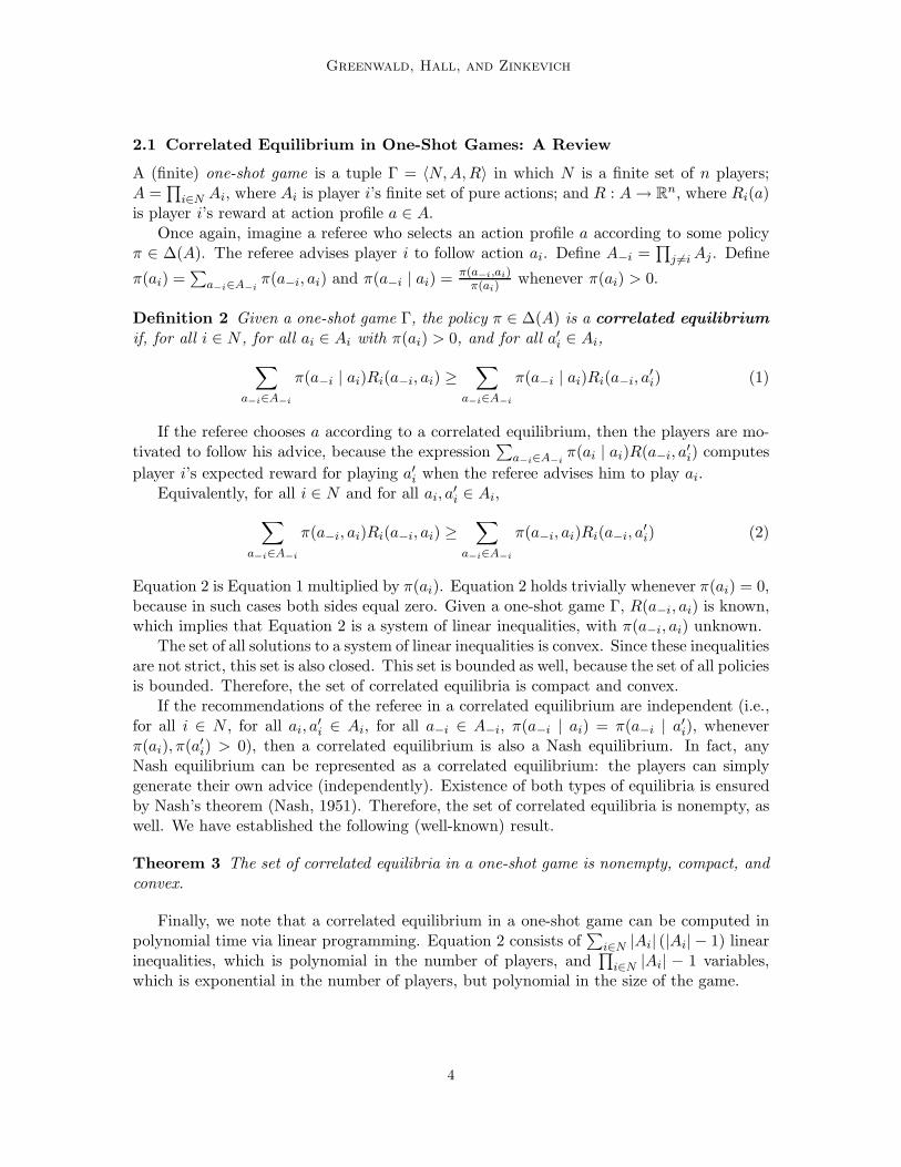
Definition 2 Given a one-shot game Γ, the policy π ∈ ∆(A) is a correlated equilibrium

if, for all i ∈ N , for all ai ∈ Ai with π(ai) > 0, and for all a′i ∈ Ai,

∑

a−i∈A−i

π(a−i | ai)Ri(a−i, ai) ≥∑

a−i∈A−i

π(a−i | ai)Ri(a−i, a′i) (1)

If the referee chooses a according to a correlated equilibrium, then the players are mo-tivated to follow his advice, because the expression

∑

a−i∈A−iπ(ai | ai)R(a−i, a

′i) computes

player i’s expected reward for playing a′i when the referee advises him to play ai.Equivalently, for all i ∈ N and for all ai, a

′i ∈ Ai,

∑

a−i∈A−i

π(a−i, ai)Ri(a−i, ai) ≥∑

a−i∈A−i

π(a−i, ai)Ri(a−i, a′i) (2)

Equation 2 is Equation 1 multiplied by π(ai). Equation 2 holds trivially whenever π(ai) = 0,because in such cases both sides equal zero. Given a one-shot game Γ, R(a−i, ai) is known,which implies that Equation 2 is a system of linear inequalities, with π(a−i, ai) unknown.

The set of all solutions to a system of linear inequalities is convex. Since these inequalitiesare not strict, this set is also closed. This set is bounded as well, because the set of all policiesis bounded. Therefore, the set of correlated equilibria is compact and convex.

If the recommendations of the referee in a correlated equilibrium are independent (i.e.,for all i ∈ N , for all ai, a

′i ∈ Ai, for all a−i ∈ A−i, π(a−i | ai) = π(a−i | a′i), whenever

π(ai), π(a′i) > 0), then a correlated equilibrium is also a Nash equilibrium. In fact, anyNash equilibrium can be represented as a correlated equilibrium: the players can simplygenerate their own advice (independently). Existence of both types of equilibria is ensuredby Nash’s theorem (Nash, 1951). Therefore, the set of correlated equilibria is nonempty, aswell. We have established the following (well-known) result.

Theorem 3 The set of correlated equilibria in a one-shot game is nonempty, compact, andconvex.

Finally, we note that a correlated equilibrium in a one-shot game can be computed inpolynomial time via linear programming. Equation 2 consists of

∑

i∈N |Ai| (|Ai| − 1) linearinequalities, which is polynomial in the number of players, and

∏

i∈N |Ai| − 1 variables,which is exponential in the number of players, but polynomial in the size of the game.

4


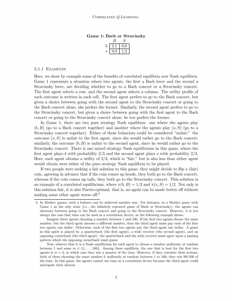
Game 1: Bach or Stravinsky

B Sb 2,1 0,0s 0,0 1,2

2.1.1 Examples

Here, we show by example some of the benefits of correlated equilibria over Nash equilibria.Game 1 represents a situation where two agents, the first a Bach lover and the second aStravinsky lover, are deciding whether to go to a Bach concert or a Stravinsky concert.The first agent selects a row, and the second agent selects a column. The utility profile ofeach outcome is written in each cell. The first agent prefers to go to the Bach concert, butgiven a choice between going with the second agent to the Stravinsky concert or going tothe Bach concert alone, she prefers the former. Similarly, the second agent prefers to go tothe Stravinsky concert, but given a choice between going with the first agent to the Bachconcert or going to the Stravinsky concert alone, he too prefers the former.

In Game 1, there are two pure strategy Nash equilibria: one where the agents play(b,B) (go to a Bach concert together) and another where the agents play (s, S) (go to aStravinsky concert together). Either of these behaviors could be considered “unfair:” theoutcome (s, S) is unfair to the first agent, since she would rather go to the Bach concert;similarly, the outcome (b,B) is unfair to the second agent, since he would rather go to theStravinsky concert. There is one mixed strategy Nash equilibrium in this game, where thefirst agent plays b with probability 2/3 and the second agent plays s with probability 2/3.Here, each agent obtains a utility of 2/3, which is “fair,” but is also less than either agentwould obtain were either of the pure strategy Nash equilibria to be played.

If two people were seeking a fair solution to this game, they might decide to flip a (fair)coin, agreeing in advance that if the coin comes up heads, they both go to the Bach concert,whereas if the coin comes up tails, they both go to the Stravinsky concert. This solution isan example of a correlated equilibrium, where π(b,B) = 1/2 and π(s, S) = 1/2. Not only isthis solution fair, it is also Pareto-optimal, that is, no agent can be made better off withoutmaking some other agent worse off.3

3. In Markov games, such a balance can be achieved another way. For instance, in a Markov game withGame 1 as the only state (i.e., the infinitely repeated game of Bach or Stravinsky), the agents canalternate between going to the Bach concert and going to the Stravinsky concert. However, it is notalways the case that time can be used as a correlation device, as the following example shows.

Imagine three agents choosing a number between 1 and 100. If the first two agents choose the samenumber, but the third agent chooses a different number, then the third agent must pay each of the firsttwo agents one dollar. Otherwise, each of the first two agents pay the third agent one dollar. A gamein this spirit is played by a quarterback (the first agent), a wide receiver (the second agent), and anopposing cornerback (the third agent): the quarterback and the wide receiver must agree upon a passingpattern which the opposing cornerback must guess.

Now, observe that it is a Nash equilibrium for each agent to choose a number uniformly at randombetween 1 and some m ∈ {1, . . . , 100}. Among these equilibria, the one that is best for the first twoagents is m = 2, in which case they win a quarter of the time. However, if they correlate their actions,both of them choosing the same number k uniformly at random between 1 to 100, they win 99/100 ofthe time. In this game, the agents cannot use time as a correlation device because the third agent couldanticipate their choices.

5


Game 2: Shapley’s Game

R P Sr 0,0 0,1 1,0p 1,0 0,0 0,1s 0,1 1,0 0,0

In Shapley’s Game (Game 2), both agents earn a higher utility by playing a correlatedequilibrium instead of a Nash equilibrium. (Shapley’s game differs from Rock-Paper-Scissorsonly in that in the latter the diagonal entries are (1

2 , 12).) At the unique Nash equilibrium,

each agent chooses an action uniformly at random and each agent’s expected utility is 1/3.However, if a referee selects an action profile uniformly at random from the set

{(r, P ), (r, S), (p,R), (p, S), (s,R), (s, P )}

and if the two agents follow the referee’s advice, then each agent’s expected utility is 1/2.Initially, one might think that the referee could select uniformly at random from, say{(r, P ), (p,R)}. But then, if the first agent were advised to play r, she could infer thatthe second agent was advised to play P , which would motivate her to play s. If one agentwere to cooperate with the referee, the other agent would be motivated to deviate.

By playing a correlated equilibrium in the Bach or Stravinsky game, the agents achievea fair and Pareto-optimal solution. In Shapley’s game, by playing a correlated rather thana Nash equilibrium, all of the agents fare better. In addition, a correlated equilibriumin a one-shot game can be computed in polynomial time. The corresponding complexityquestion for Nash equilibrium is open, although it is known that it is NP-hard to computecertain classes of Nash equilibria (Gilboa and Zemel, 1989; Conitzer and Sandholm, 2003).

2.2 Correlated Equilibrium Policies in Markov Games

We are now ready to address the question of whether or not agents are willing to followthe advice of a referee in a Markov game. To do so, we compute the expected utility of anagent when it follows the advice of the referee as well as the expected utility of an agentwhen it deviates, in both cases assuming all other agents follow the advice of the referee.

Given a Markov game Γγ , and a referee’s policy π, consider the transition matrix T π suchthat T π

ss′ is the probability of transitioning to state s′ from state s, given that the refereeselects an action profile according to the distribution πs that the agents indeed follow:

T πss′ =

∑

a∈A(s)

πs(a)P [s′ | s, a] (3)

Exponentiating this matrix, the probability of transitioning to state s′ from state s after ttime steps is given by (T π

ss′)t. Now the value function V π

i (s) represents agent i’s expectedreward, originating at state s, assuming all agents follow the referee’s policy π:

V πi (s) = (1 − γ)

∞∑

t=0

∑

s′∈S

γt(T πss′)

t∑

a∈A(s′)

πs′(a)Ri(s′, a) (4)

6


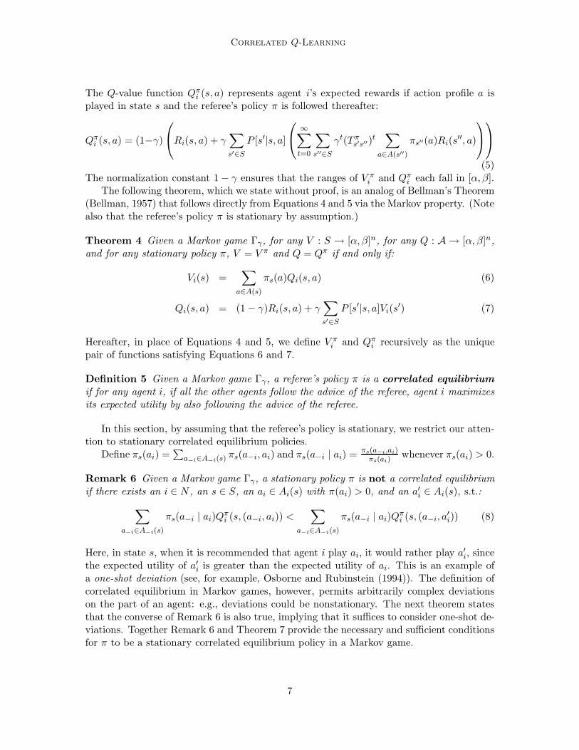
The Q-value function Qπi (s, a) represents agent i’s expected rewards if action profile a is

played in state s and the referee’s policy π is followed thereafter:

Qπi (s, a) = (1−γ)

Ri(s, a) + γ∑

s′∈S

P [s′|s, a]

∞∑

t=0

∑

s′′∈S

γt(T πs′s′′)

t∑

a∈A(s′′)

πs′′(a)Ri(s′′, a)

(5)The normalization constant 1 − γ ensures that the ranges of V π

i and Qπi each fall in [α, β].

The following theorem, which we state without proof, is an analog of Bellman’s Theorem(Bellman, 1957) that follows directly from Equations 4 and 5 via the Markov property. (Notealso that the referee’s policy π is stationary by assumption.)

Theorem 4 Given a Markov game Γγ, for any V : S → [α, β]n, for any Q : A → [α, β]n,and for any stationary policy π, V = V π and Q = Qπ if and only if:

Vi(s) =∑

a∈A(s)

πs(a)Qi(s, a) (6)

Qi(s, a) = (1 − γ)Ri(s, a) + γ∑

s′∈S

P [s′|s, a]Vi(s′) (7)

Hereafter, in place of Equations 4 and 5, we define V πi and Qπ

i recursively as the uniquepair of functions satisfying Equations 6 and 7.

Definition 5 Given a Markov game Γγ, a referee’s policy π is a correlated equilibrium

if for any agent i, if all the other agents follow the advice of the referee, agent i maximizesits expected utility by also following the advice of the referee.

In this section, by assuming that the referee’s policy is stationary, we restrict our atten-tion to stationary correlated equilibrium policies.

Define πs(ai) =∑

a−i∈A−i(s)πs(a−i, ai) and πs(a−i | ai) = πs(a−i,ai)

πs(ai)whenever πs(ai) > 0.

Remark 6 Given a Markov game Γγ, a stationary policy π is not a correlated equilibriumif there exists an i ∈ N , an s ∈ S, an ai ∈ Ai(s) with π(ai) > 0, and an a′i ∈ Ai(s), s.t.:

∑

a−i∈A−i(s)

πs(a−i | ai)Qπi (s, (a−i, ai)) <

∑

a−i∈A−i(s)

πs(a−i | ai)Qπi (s, (a−i, a

′i)) (8)

Here, in state s, when it is recommended that agent i play ai, it would rather play a′i, sincethe expected utility of a′i is greater than the expected utility of ai. This is an example ofa one-shot deviation (see, for example, Osborne and Rubinstein (1994)). The definition ofcorrelated equilibrium in Markov games, however, permits arbitrarily complex deviationson the part of an agent: e.g., deviations could be nonstationary. The next theorem statesthat the converse of Remark 6 is also true, implying that it suffices to consider one-shot de-viations. Together Remark 6 and Theorem 7 provide the necessary and sufficient conditionsfor π to be a stationary correlated equilibrium policy in a Markov game.

7


Theorem 7 Given a Markov game Γγ , a stationary policy π is a correlated equilibrium iffor all i ∈ N , for all s ∈ S, for all ai ∈ Ai(s) with π(ai) > 0, for all a′i ∈ Ai(s),

∑

a−i∈A−i(s)

πs(a−i | ai)Qπi (s, (a−i, ai)) ≥

∑

a−i∈A−i(s)

πs(a−i | ai)Qπi (s, (a−i, a

′i)) (9)

Here, in state s, when it is recommended that agent i play ai, it is happy to play ai, becausethe expected utility of ai is greater than or equal to the expected utility of a′i, for all a′i.

Observe the following: if all of the other agents but agent i play according to the referee’spolicy π, then from the point of view of agent i, its environment is an MDP. Hence, theone-shot deviation principle for MDPs establishes Theorem 7 (see, for example, (Greenwaldand Zinkevich, 2005)).

Corollary 8 Given a Markov game Γγ, a stationary policy π is a correlated equilibrium iffor all i ∈ N , for all s ∈ S, and for all ai, a

′i ∈ Ai(s),

∑

a−i∈A−i(s)

πs(a−i, ai)Qπi (s, (a−i, ai)) ≥

∑

a−i∈A−i(s)

πs(a−i, ai)Qπi (s, (a−i, a

′i)) (10)

Equation 10 is Equation 9 multiplied by πs(ai).Unlike in one-shot games where only the π(a−i, ai)’s are unknown (see Equation 2), here

the πs(a−i, ai)’s, and hence the Qπi (s, (a−i, ai))’s, are unknown. In particular, Equation 10

is not a system of linear inequalities, but rather a system of nonlinear inequalities. Next, wepropose a class of iterative algorithms, based on the correlated equilibrium solution concept,and we investigate the question of whether or not any algorithms in this class converge tocorrelated equilibrium policies in Markov games, effectively solving this nonlinear system.

3. Multiagent Q-Learning

In a companion paper (Greenwald and Zinkevich, 2005), we rely on Kakutani’s fixed pointtheorem to establish the existence of stationary correlated equilibrium policies in Markovgames. Specifically, we define a correspondence, the fixed points of which are the stationarycorrelated equilibrium policies of a Markov game, and we show that this correspondence sat-isfies Kakutani’s sufficient conditions, ensuring that the set of such fixed points is nonempty.

The definition of this correspondence suggests an algorithm for computing one of its fixedpoints, that is, a global equilibrium policy, based on local updates: given initial Q-valuesand an initial policy, update the values, Q-values, and policy at each state, and repeat. Inthe remainder of this paper, we investigate the question of whether or not instances of thisprocedure converge to correlated equilibrium policies in Markov games.

In MDPs, the special case of Markov games with only a single agent, the correspondinglocal update procedure, known as value iteration, is well-known: Given Q-values at time tfor all s ∈ S and for all a ∈ A(s), namely Qt(s, a), at time t + 1,

V t+1(s) := maxa∈A(s)

Qt(s, a) (11)

Qt+1(s, a) := (1 − γ)R(s, a) + γ∑

s′∈S

P [s′|s, a]V t+1(s′) (12)

8


This procedure converges to a unique fixed point V ∗, a unique fixed point Q∗, and a globallyoptimal policy π∗, which is not necessarily unique (e.g., see Puterman (1994)).

More generally, in Markov games, given Q-values at time t for all i ∈ N , for all s ∈ S,and for all a ∈ A(s), namely Qt

i(s, a); given a policy πt; and given a selection mechanism

f , that is, a mapping from one-shot games into (sets of) joint distributions; at time t + 1,

V t+1i (s) :=

∑

a∈A(s)

πts(a)Qt

i(s, a) (13)

Qt+1i (s, a) := (1 − γ)Ri(s, a) + γ

∑

s′∈S

P [s′|s, a]V t+1i (s′) (14)

πt+1s ∈ f(Qt+1(s)) (15)

We now proceed to investigate the question of whether or not this procedure converges toequilibrium policies in Markov games, for various choices of the selection mechanism f .

Following the literature on this subject (e.g., Littman (1994, 2001); Hu and Wellman(2003)), we experiment with “correlated-Q learning,” in which values and Q-values areupdated asynchronously (see Tables 1 and 2), rather than “correlated value iteration,” inwhich these values are updated synchronously, as suggested by Equations 13, 14, and 15.

Finally, one important application-specific issue arises: can we assume the existence ofa trusted third party who can act as a centralized coordinator? Or need we decentralizethe implementation of multiagent value iteration and Q-learning? We present two genericformulations of multiagent Q-learning: the first is centralized; the second is decentralized.

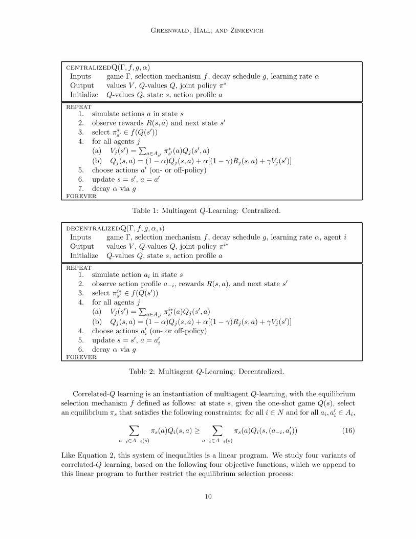
3.1 Centralized Multiagent Learning

The generalization of dynamic programming and reinforcement learning from MDPs toMarkov games is straightforward, if one assumes the existence of a trusted third party whoserves as a central coordinator. A template for centralized multiagent Q-learning, is shownin Table 1. Notably, in Step 3, the central coordinator, who has knowledge of all agents’Q-tables, selects a joint distribution on which the agents updates in Step 4 rely.

3.2 Decentralized Multiagent Learning

Rather than rely on a central coordinator, Hu and Wellman (2003) assume that each agentcan observe all the other agents’ actions and rewards. With this assumption, one candecentralize the implementation of multiagent Q-learning, as shown in Table 2. Here, inStep 3, each agent selects a joint distribution on which to base its updates in Step 4. Doingso requires knowledge of all agents’ Q-tables. By observing the actions and rewards of theother agents in Step 2, sufficient information is available to perform this updating exactlyas the central coordinator would in the centralized version of multiagent Q-learning.

3.3 Correlated-Q Learning

Recall that a selection mechanism f is a mapping from one-shot games into (sets of) jointdistributions. In particular, an equilibrium selection mechanism selects an equilibrium. Forexample, a correlated equilibrium selection mechanism, given a one-shot game, returns a(set of) joint distributions that satisfies Equation 1 (or, equivalently, Equation 2).

9


centralizedQ(Γ, f, g, α)Inputs game Γ, selection mechanism f , decay schedule g, learning rate αOutput values V , Q-values Q, joint policy π∗

Initialize Q-values Q, state s, action profile a

repeat1. simulate actions a in state s2. observe rewards R(s, a) and next state s′

3. select π∗s′ ∈ f(Q(s′))

4. for all agents j(a) Vj(s

′) =∑

a∈As′

π∗s′(a)Qj(s

′, a)

(b) Qj(s, a) = (1 − α)Qj(s, a) + α[(1 − γ)Rj(s, a) + γVj(s′)]

5. choose actions a′ (on- or off-policy)6. update s = s′, a = a′

7. decay α via gforever

Table 1: Multiagent Q-Learning: Centralized.

decentralizedQ(Γ, f, g, α, i)Inputs game Γ, selection mechanism f , decay schedule g, learning rate α, agent iOutput values V , Q-values Q, joint policy πi∗

Initialize Q-values Q, state s, action profile a

repeat1. simulate action ai in state s2. observe action profile a−i, rewards R(s, a), and next state s′

3. select πi∗s′ ∈ f(Q(s′))

4. for all agents j(a) Vj(s

′) =∑

a∈As′

πi∗s′ (a)Qj(s

′, a)

(b) Qj(s, a) = (1 − α)Qj(s, a) + α[(1 − γ)Rj(s, a) + γVj(s′)]

4. choose actions a′i (on- or off-policy)5. update s = s′, a = a′i6. decay α via g

forever

Table 2: Multiagent Q-Learning: Decentralized.

Correlated-Q learning is an instantiation of multiagent Q-learning, with the equilibriumselection mechanism f defined as follows: at state s, given the one-shot game Q(s), selectan equilibrium πs that satisfies the following constraints: for all i ∈ N and for all ai, a

′i ∈ Ai,

∑

a−i∈A−i(s)

πs(a)Qi(s, a) ≥∑

a−i∈A−i(s)

πs(a)Qi(s, (a−i, a′i)) (16)

Like Equation 2, this system of inequalities is a linear program. We study four variants ofcorrelated-Q learning, based on the following four objective functions, which we append tothis linear program to further restrict the equilibrium selection process:

10


1. utilitarian: maximize the sum of all agents’ rewards: at state s,

maxπs∈∆(A(s))

∑

j∈N

∑

a∈A(s)

πs(a)Qj(s, a) (17)

2. egalitarian: maximize the minimum of all agents’ rewards: at state s,

maxπs∈∆(A(s))

minj∈N

∑

a∈A(s)

πs(a)Qj(s, a) (18)

3. plutocratic: maximize the maximum of all agents’ rewards: at state s,

maxπs∈∆(A(s))

maxj∈N

∑

a∈A(s)

πs(a)Qj(s, a) (19)

4. dictatorial: maximize the maximum of any individual agent’s rewards: for agent i andat state s,

maxπs∈∆(A(s))

∑

a∈A(s)

πs(a)Qi(s, a) (20)

In our experimental discussion, we abbreviate these variants of correlated-Q (CE-Q)learning as uCE-Q, eCE-Q, pCE-Q, and dCE-Q, respectively. Three out of four of ourimplementations of CE-Q learning are centralized: uCE-Q, eCE-Q, and pCE-Q learning;however, dCE-Q learning is decentralized: each agent i learns as if it is the dictator.

3.4 Experimental Setup

In the next several sections, we describe experiments with various multiagent Q-learningalgorithms on a standard test bed of Markov games, including the “grid games” as wellas grid soccer. In doing so, we compare the performance of correlated-Q learning withother well-known multiagent Q-learning algorithms described in the literature: specifically,Q-learning (Watkins, 1989), minimax-Q (or foe-Q) learning (Littman, 1994), friend-Q learn-ing (Littman, 2001), and two variants of Nash-Q learning (Hu and Wellman, 2003). Weinvestigate the question of whether or not these multiagent Q-learning algorithms convergeto equilibrium policies in general-sum Markov games.

In an environment of multiple learners, off-policy Q-learners are unlikely to converge toan equilibrium policy. Each agent would learn a best-response to the random behavior ofthe other agents, rather than a best-response to intelligent behavior on the part of the otheragents. Hence, as a first point of comparison, we implemented on-policy Q-learning (Suttonand Barto, 1998). Moreover, in our implementation of Q-learning, if ever the optimal actionis not unique, an agent randomizes uniformly among all its optimal actions. Otherwise, Q-learning can easily perform arbitrarily badly in games with multiple coordination equilibria,all of equivalent value, by failing to coordinate their behavior.

In addition, we implemented centralized and decentralized versions of Nash-Q learning.We refer to these two algorithms as coordinated Nash-Q (cNE-Q) and best Nash-Q (bNE-Q),respectively. In the former, a central coordinator selects and broadcasts a Nash equilibrium

11


A B

A

A B A B

B A,B A,B

(a) Grid Game 1 (b) Grid Game 2 (c) Grid Game 3

Figure 1: Grid games: Initial States and Sample Equilibria. Shapes indicate goals.

to all agents; in the latter, each agent independently selects that Nash equilibrium whichmaximizes its utility. Lastly, we implemented decentralized versions of foe-Q and friend-Q.In our implementations of foe-Q, friend-Q, and best Nash-Q, we allow the agents to observetheir opponents Q-values. In our implementation of coordinated Nash-Q, it suffices for thecentral coordinator to observe all agents Q-values.

4. Grid Games

The first set of detailed experimental results on which we report pertain to grid games. Wedescribe three grid games, all of which are two-player, general-sum Markov games: grid game1 (GG1) (Hu and Wellman, 2003), a multi-state coordination game; grid game 2 (GG2) (Huand Wellman, 2003), a stochastic game that is reminiscent of Bach or Stravinsky; and gridgame 3 (GG3) (Greenwald and Hall, 2003), a multi-state version of Chicken.4 In fact, onlyGG2 is inherently stochastic. In the next section, we describe experiments with a simpleversion of soccer, a two-player, zero-sum Markov game, that is highly stochastic.

Figure 1 depicts the initial states of GG1, GG2, and GG3. All three games involvetwo agents and two (possibly overlapping) goals. If ever an agent reaches its goal, it scoressome points, and the game ends. The agents’ action sets include one step in any of the fourcompass directions. Actions are executed simultaneously, which implies that both agentscan score in the same game instance. If both agents attempt to move into the same celland this cell is not an overlapping goal, their moves fail (that is, the agents positions do notchange), and they both lose 1 point in GG1 and GG2 and 50 points in GG3.

In GG1, there are two distinct goals, each worth 100 points. In GG2, there is one goalworth 100 points and two barriers: if an agent attempts to move through one of the barriers,then with probability 1/2 this move fails. In GG3, like GG2, there is one goal worth 100points, but there are no stochastic transitions and the reward structure differs: At the start,if both agents avoid the center state by moving up the sides, they are each rewarded with20 points; in addition, any agent that chooses the center state is rewarded with 25 points(NB: if both agents choose the center state, they collide, each earning −25 = 25 − 50).

4. Chicken is a game played by two people driving cars. Each driver can either drive straight ahead, andrisk his life, or swerve out of the way, and risk embarrassment.

12


4.1 Grid Game Equilibria

In all three grid games, there exist pure strategy stationary correlated, and hence Nash,equilibrium policies for both agents. In GG1, there are several pairs of pure strategyequilibrium policies in which the agents coordinate their behavior (see Hu and Wellman(2003) for graphical depictions). In GG2 and GG3, there are exactly two pure strategyequilibrium policies: one agent moves up the center and the other moves up the side, andthe same again with the agents’ roles reversed. These equilibria are asymmetric: in GG2,the agent that moves up the center scores 100, but the agent that moves up the sides scoresonly 50 on average (due to the 50% chance of crossing the barrier); in GG3, the agent thatmoves up the center scores 125, but the agent that moves up the sides scores only 100.

Since there are multiple pure strategy stationary equilibrium policies in these grid games,it is possible to construct additional stationary equilibrium policies as convex combinationsof the pure policies. In GG2, there exists a continuum of symmetric correlated equilibriumpolicies: i.e., for all p ∈ [0, 1], with probability p one agent moves up the center and theother attempts to pass through the barrier, and with probability 1 − p the agents’ rolesare reversed. In GG3, there exists a symmetric correlated equilibrium policy in which bothagents move up the sides with high probability and each of the pure strategy equilibriumpolicies is played with equally low probability. Do multiagent Q-learners learn to play thesestationary equilibrium policies? We investigate this question presently.

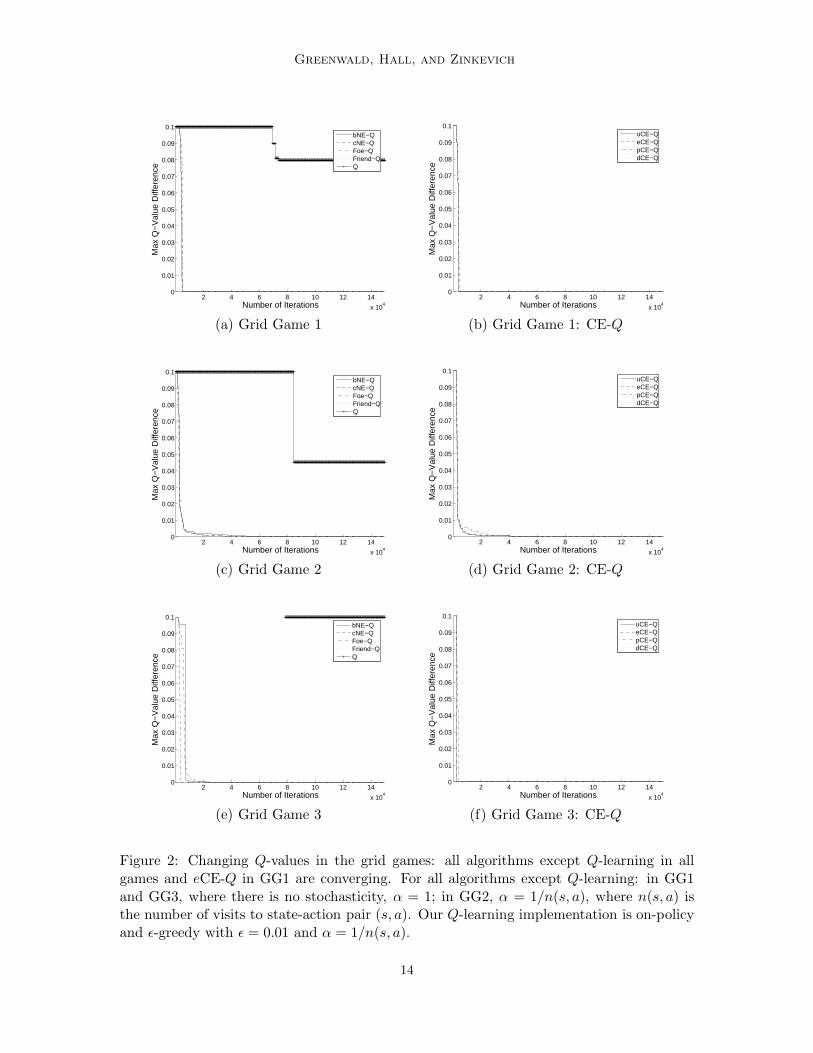
4.2 Empirical Convergence

Our experiments reveal that all of the multiagent Q-learning algorithms are converging inthe three grid games. However, Q-learning does not converge in the grid games. Littman(2001) proves that FF-Q converges in general-sum Markov games. Hu and Wellman (2003)show empirically that NE-Q converges in both GG1 and GG2. Figure 2 shows that NE-Qis also converging in GG3. Similarly, CE-Q converges in all three grid games. We cannot,however, make any claims about the convergence of CE-Q in general.

The values plotted in Figure 2 are computed as follows. Define an error term errti at

time t for agent i as the difference between Q(st, at) at time t and Q(st, at) at time t − 1:i.e., errt

i =∣

∣Qti(s

t, at) − Qt−1i (st, at)

∣

∣. The error values on the y-axis depict the maximumerror from the current time x to the end of the simulation T : i.e., maxt=x,...,T errt

i, fori = 1. The values on the x-axis, representing time, range from 1 to T ′, for some T ′ < T .5 Inour experiments, we set T ′ = 1.5× 105 and T = 2× 105. The maximum change in Q-valuesis converging to 0 for all algorithms except Q-learning in all games.

In our experiments, the parameters are set as follows. Our implementation of Q-learningis on-policy and ε-greedy, with ε = 0.01 and α = 1/n(s, a), where n(s, a) is the number ofvisits to state-action pair (s, a). All other algorithms are off-policy (equivalently, on-policyand ε-greedy with ε = 1). For these off-policy learning algorithms, in GG1 and GG3, wherethere is no stochasticity, α = 1; in GG2, however, like Q-learning, α = 1/n(s, a). Finally,γ = 0.9 in all cases. Next, we investigate the policies learned by the algorithms.

5. Setting T ′ = T is sometimes misleading: It could appear that non-convergent algorithms are converging,because our metric measures the maximum error between the current time and the end of the simulation,but it could be that the change in Q-values is negligible for all states visited at the end of the simulation.

13


2 4 6 8 10 12 14

x 104

0

0.01

0.02

0.03

0.04

0.05

0.06

0.07

0.08

0.09

0.1

Number of Iterations

Max

Q−

Val

ue D

iffer

ence

bNE−QcNE−QFoe−QFriend−QQ

2 4 6 8 10 12 14

x 104

0

0.01

0.02

0.03

0.04

0.05

0.06

0.07

0.08

0.09

0.1


Max

Q−

Val

ue D

iffer

ence

uCE−QeCE−QpCE−QdCE−Q

(a) Grid Game 1 (b) Grid Game 1: CE-Q

2 4 6 8 10 12 14

x 104

0

0.01

0.02

0.03

0.04

0.05

0.06

0.07

0.08

0.09

0.1


Max

Q−

Val

ue D

iffer

ence


2 4 6 8 10 12 14

x 104

0

0.01

0.02

0.03

0.04

0.05

0.06

0.07

0.08

0.09

0.1


Max

Q−

Val

ue D

iffer

ence


(c) Grid Game 2 (d) Grid Game 2: CE-Q

2 4 6 8 10 12 14

x 104

0

0.01

0.02

0.03

0.04

0.05

0.06

0.07

0.08

0.09

0.1


Max

Q−

Val

ue D

iffer

ence


2 4 6 8 10 12 14

x 104

0

0.01

0.02

0.03

0.04

0.05

0.06

0.07

0.08

0.09

0.1


Max

Q−

Val

ue D

iffer

ence


(e) Grid Game 3 (f) Grid Game 3: CE-Q

Figure 2: Changing Q-values in the grid games: all algorithms except Q-learning in allgames and eCE-Q in GG1 are converging. For all algorithms except Q-learning: in GG1and GG3, where there is no stochasticity, α = 1; in GG2, α = 1/n(s, a), where n(s, a) isthe number of visits to state-action pair (s, a). Our Q-learning implementation is on-policyand ε-greedy with ε = 0.01 and α = 1/n(s, a).

14


4.3 Equilibrium Policies

We now address the question: what is it that the Q-learning algorithms learn? In summary,

• Q-learning does not converge, and it does not learn equilibrium policies;

• friend-Q and foe-Q learning converge, but need not learn equilibrium policies;

• NE-Q and CE-Q learn equilibrium policies, whenever they converge.

To address this question, we analyzed the agents’ policies at the end of each simulationby appending to the learning phase an auxiliary testing phase in which the agents playaccording to the policies they learned. Our learning phase is randomized: not only arethe state transitions stochastic, on-policy Q-learners and off-policy multiagent Q-learnerscan all make probabilistic decisions. Thus, if there exist multiple equilibrium policies in agame, agents can learn different equilibrium policies across different runs. Moreover, sinceagents can learn stochastic policies, scores can vary across different test runs. Nonetheless,we presented only one run of the learning phase (see Section 4.2) and here we present onlyone test run, each of which is representative of their respective sets of possible outcomes.

The results of our testing phase, during which the agents played the grid games repeat-edly, are depicted in Table 3. Foe-Q learners perform poorly in GG1. Rather than progresstoward the goal, they cower in the corners, avoiding collisions, and consequently avoidingthe goal. Sometimes one agent simply moves out of the way of the other, allowing its oppo-nent to reach its goal rather than risk collision. In GG2 and GG3, the principle of avoidingcollisions leads both foe-Q learners straight up the sides of the grid. Although these policiesyield reasonable scores in GG2, and Pareto optimal scores in GG3, these are not equilibriumpolicies. On the contrary, foe-Q learning yields policies that are not rational—both agentshave an incentive to deviate to the center, since the reward for using the center passageexceeds that of moving up the sides, given that one’s opponent is moving up the side.

In GG1, friend-Q learning can perform even worse than foe-Q learning. This result mayappear surprising at first glance, since GG1 satisfies the conditions under which friend-Qlearning is guaranteed to converge to an equilibrium policy (Littman, 2001). Indeed, friend-Q learns Q-values that support equilibrium policies, but in our decentralized implementationof friend-Q learning, friends lack the ability to coordinate their play. Whenever these so-called “friends” choose policies that collide, both agents obtain negative scores for theremainder of the simulation: e.g., if the agents’ policies lead them to one another’s goals,both agents move towards the center ever after. In our experiments, friend-Q learned astochastic policy6 at the start state that allowed it to complete a few games successfullybefore arriving at a state where the friendly assumption led the players to collide indefinitely.In GG2 and GG3, friend-Q’s performance is always poor: both agents learn equilibriumpolicies that use the center passage, which leads to repeated collisions.

On-policy Q-learning is not successful in the grid games: it learns equilibrium policiesin GG1, but in GG2, it learns a foe-Q-like (non-equilibrium) policy.7 As expected, we have

6. Like Q-learning, in our implementation of friend-Q learning, if ever the optimal action is not unique, anagent randomizes uniformly among all its optimal actions.

7. Although Q-learning did not converge in the grid games, the policies appeared stable at the end of thelearning phase. By decaying α, we disallow large changes in the agents’ Q-values, which makes changesin their policies less and less frequent.

15


GG1 Avg. Score Games Convergence? Eqm. Values? Eqm. Play?

Q 100,100 2500 No Yes YesFoe-Q 0,0 0 Yes No NoFriend-Q −3239,−3239 3 Yes Yes No

uCE-Q 100,100 2500 Yes Yes YeseCE-Q 100,100 2500 Yes Yes YespCE-Q 100,100 2500 Yes Yes YescNE-Q 100,100 2500 Yes Yes Yes

dCE-Q −104,−104 0 Yes Yes NobNE-Q −104,−104 0 Yes Yes No


Q 67.3,66.2 3008 No No NoFoe-Q 65.9,67.4 3011 Yes No NoFriend-Q −104,−104 0 Yes No No

uCE-Q 50.4,100 3333 Yes Yes YeseCE-Q 49.5,100 3333 Yes Yes YespCE-Q 50.3,100 3333 Yes Yes YescNE-Q 100,50.2 3333 Yes Yes Yes

dCE-Q 49.9,100 3333 Yes Yes YesbNE-Q 100,49.7 3333 Yes Yes Yes


Q 62.6,95.4 3314 No No NoFoe-Q 120,120 3333 Yes No NoFriend-Q −25 × 104,−25 × 104 0 Yes No No

uCE-Q 117,117 3333 Yes Yes YeseCE-Q 117,117 3333 Yes Yes YespCE-Q 100,125 3333 Yes Yes YescNE-Q 125,100 3333 Yes Yes Yes

dCE-Q −25 × 104,−25 × 104 0 Yes Yes NobNE-Q −25 × 104,−25 × 104 0 Yes Yes No

Table 3: Testing phase: Grid games played repeatedly. Average scores across 104 movesare shown. The number of games played varied with the agents’ policies: sometimes agentsmoved directly to the goal; other times they digressed. For each learning algorithm, theConvergence? column states whether or not the Q-values converge; the Equilibrium Values?column states whether or not the Q-values correspond to an equilibrium policy; the Equilib-rium Play? column states whether or not the trajectories of play during testing correspondto an equilibrium policy.

16


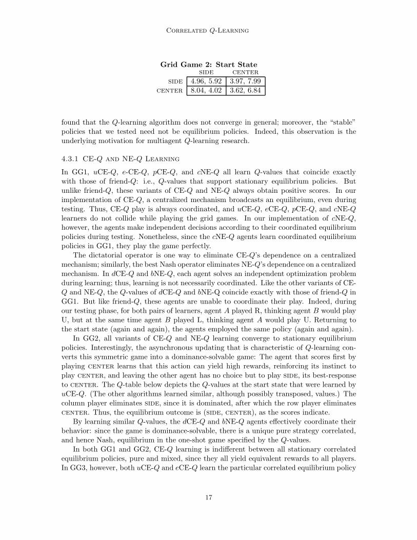
Grid Game 2: Start Stateside center

side 4.96, 5.92 3.97, 7.99center 8.04, 4.02 3.62, 6.84

found that the Q-learning algorithm does not converge in general; moreover, the “stable”policies that we tested need not be equilibrium policies. Indeed, this observation is theunderlying motivation for multiagent Q-learning research.

4.3.1 CE-Q and NE-Q Learning

In GG1, uCE-Q, e-CE-Q, pCE-Q, and cNE-Q all learn Q-values that coincide exactlywith those of friend-Q: i.e., Q-values that support stationary equilibrium policies. Butunlike friend-Q, these variants of CE-Q and NE-Q always obtain positive scores. In ourimplementation of CE-Q, a centralized mechanism broadcasts an equilibrium, even duringtesting. Thus, CE-Q play is always coordinated, and uCE-Q, eCE-Q, pCE-Q, and cNE-Qlearners do not collide while playing the grid games. In our implementation of cNE-Q,however, the agents make independent decisions according to their coordinated equilibriumpolicies during testing. Nonetheless, since the cNE-Q agents learn coordinated equilibriumpolicies in GG1, they play the game perfectly.

The dictatorial operator is one way to eliminate CE-Q’s dependence on a centralizedmechanism; similarly, the best Nash operator eliminates NE-Q’s dependence on a centralizedmechanism. In dCE-Q and bNE-Q, each agent solves an independent optimization problemduring learning; thus, learning is not necessarily coordinated. Like the other variants of CE-Q and NE-Q, the Q-values of dCE-Q and bNE-Q coincide exactly with those of friend-Q inGG1. But like friend-Q, these agents are unable to coordinate their play. Indeed, duringour testing phase, for both pairs of learners, agent A played R, thinking agent B would playU, but at the same time agent B played L, thinking agent A would play U. Returning tothe start state (again and again), the agents employed the same policy (again and again).

In GG2, all variants of CE-Q and NE-Q learning converge to stationary equilibriumpolicies. Interestingly, the asynchronous updating that is characteristic of Q-learning con-verts this symmetric game into a dominance-solvable game: The agent that scores first byplaying center learns that this action can yield high rewards, reinforcing its instinct toplay center, and leaving the other agent has no choice but to play side, its best-responseto center. The Q-table below depicts the Q-values at the start state that were learned byuCE-Q. (The other algorithms learned similar, although possibly transposed, values.) Thecolumn player eliminates side, since it is dominated, after which the row player eliminatescenter. Thus, the equilibrium outcome is (side, center), as the scores indicate.

By learning similar Q-values, the dCE-Q and bNE-Q agents effectively coordinate theirbehavior: since the game is dominance-solvable, there is a unique pure strategy correlated,and hence Nash, equilibrium in the one-shot game specified by the Q-values.

In both GG1 and GG2, CE-Q learning is indifferent between all stationary correlatedequilibrium policies, pure and mixed, since they all yield equivalent rewards to all players.In GG3, however, both uCE-Q and eCE-Q learn the particular correlated equilibrium policy

17


that yields symmetric scores, because both the sum and the minimum of the agents’ rewardsat this equilibrium exceed those of any other equilibrium policies. Consequently, the sumof the scores of uCE-Q and eCE-Q exceed that of any Nash equilibrium. CE-Q’s rewardsdo not exceed the sum of the foe-Q learners’ scores, however; but foe-Q learners do notbehave rationally. Coincident with cNE-Q, the pCE-Q learning algorithm converges to apure strategy equilibrium policy that is among those policies that maximize the maximum ofall agents’ rewards. Finally, each dCE-Q and bNE-Q agent attempts to play the equilibriumpolicy that maximizes its own rewards, yielding repeated collisions and negative scores.

5. Soccer Game

The grid games are general-sum Markov games for which there exist pure strategy stationaryequilibrium policies. In this section, we consider a two-player, zero-sum Markov game forwhich there do not exist pure strategy equilibrium policies. Our game is a simplified versionof the soccer game that is described in Littman (1994).

The soccer field is a grid (see Figure 3). There are two players, whose possible actionsare N, S, E, W, and stick. Players choose their actions simultaneously. Actions are executedin random order. If the sequence of actions causes the players to collide, then only the firstplayer moves, and only if the cell into which he is moving is unoccupied. If the player withthe ball attempts to move into the player without the ball, then the ball changes possession;however, the player without the ball cannot steal the ball by attempting to move into theplayer with the ball.8 Finally, if the player with the ball moves into a goal, then he scores+100 if it is in fact his own goal and the other player scores −100, or he scores −100 if itis the other player’s goal and the other player scores +100. In either case, the game ends.

There are no explicit stochastic state transitions in this game’s specification. However,there are “implicit” stochastic state transitions, resulting from the fact that the playersactions are executed in random order. From each state, there are transitions to (at most)two subsequent states, each with probability 1/2. These subsequent states are: the statethat arises when player A (B) moves first and player B (A) moves second.

In this simple soccer game, there do not exist pure stationary equilibrium policies, sinceat certain states there do not exist pure strategy equilibria. For example, at the statedepicted in Figure 3 (hereafter, state s), any pure policy for player A is subject to indefiniteblocking by player B; but if player A employs a mixed policy, then player A can hope topass player B on his next move.

W E

N

S

AAAAAAA

BBB

BB

B

B

B A

Figure 3: Soccer Game. The circle represents the ball. If player A moves W, he loses theball to player B; but if player B moves E, attempting to steal the ball, he cannot.

8. This form of the game is due to Littman (1994).

18


2 4 6 8 10 12 14

x 104

0

0.01

0.02

0.03

0.04

0.05

0.06

0.07

0.08

0.09

0.1


Max

Q−

Val

ue D

iffer

ence


2 4 6 8 10 12 14

x 104

0

0.01

0.02

0.03

0.04

0.05

0.06

0.07

0.08

0.09

0.1


Max

Q−

Val

ue D

iffer

ence


(a) Grid Soccer (b) Grid Soccer: CE-Q

Figure 4: Changing Q-values in the soccer game: all algorithms are converging, except Q-learning. For all algorithms, the discount factor γ = 0.9 and the parameter α = 1/n(s, a),where n(s, a) is the number of visits to state-action pair (s, a). Our Q-learning implemen-tation is on-policy and ε-greedy with ε = 0.01.

5.1 Empirical Convergence

We experimented with the same set of algorithms in this soccer game as in the grid games.Consistent with the theory, friend-Q and foe-Q converge at all state-action pairs. Nash-Qalso converges everywhere, as do all variants of correlated-Q—in this game, all equilibria atall states have equivalent values; thus, all correlated-Q operators yield identical outcomes.Moreover, correlated-Q, like Nash-Q, learns Q-values that coincide exactly with those offoe-Q. But Q-learning, as in the grid games, does not converge.

Figure 4 shows that while the multiagent-Q learning algorithms converge, Q-learningitself does not converge. Our implementation of Q-learning is on-policy and ε-greedy, withε = 0.01. The parameter α = 1/n(s, a), where n(s, a) is the number of visits to state-actionpair (s, a). The discount factor γ = 0.9.

As in Figure 2, the y-values depict the maximum error from the current time x to theend of the simulation T : i.e., maxt=x,...,T errt

i = maxt=x,...,T

∣

∣Qti(s

t, at) − Qt−1i (st, at)

∣

∣, fori = A. The values on the x-axis, representing time, range from 1 to T ′, for some T ′ < T .As in our experiments with the grid games, we set T = 1.5 × 105 and T = 2 × 105.

Figure 5 presents an example of a state-action pair at which classic Q-learning doesnot converge. The values on the x-axis represent time, and the corresponding y-values arethe error values errt

A =∣

∣Qti(s,S,E) − Qt−1

i (s,S,E)∣

∣. In Figure 5(a), although the Q-valuedifferences are decreasing at times, they are not converging. They are decreasing onlybecause the learning rate α is decreasing. Often times, the amplitude of the oscillations inerror values is as great as the envelope of the learning rate.

Friend-Q, however, converges to a pure policy for player A at state s, namely W. Learn-ing according to friend-Q, player A fallaciously anticipates the following sequence of events:player B sticks at state s, and player A takes action W. By taking action W, player A passesthe ball to player B, with the intent that player B score for him. Player B is indifferentamong her actions, since she, again fallaciously, assumes player A plans to score a goal forher immediately.

19


0 2 4 6 8 10 12 14 16 18

x 104

0

0.1

0.2

0.3

0.4

0.5

0.6

0.7

0.8

0.9

1x 10

−3

Simulation Iteration

Q−

valu

e D

iffer

ence

Q

0 2 4 6 8 10 12 14 16 18

x 104

0

0.1

0.2

0.3

0.4

0.5

0.6

0.7

0.8

0.9

1x 10

−3


Q−

valu

e D

iffer

ence

uCE−Q

0 2 4 6 8 10 12 14 16 18

x 104

0

0.1

0.2

0.3

0.4

0.5

0.6

0.7

0.8

0.9

1x 10

−3


Q−

valu

e D

iffer

ence

dCE−Q

(a) Q-learning (b) uCE-Q (c) dCE-Q

0 2 4 6 8 10 12 14 16 18

x 104

0

0.1

0.2

0.3

0.4

0.5

0.6

0.7

0.8

0.9

1x 10

−3


Q−

valu

e D

iffer

ence

Friend−Q

0 2 4 6 8 10 12 14 16 18

x 104

0

0.1

0.2

0.3

0.4

0.5

0.6

0.7

0.8

0.9

1x 10

−3


Q−

valu

e D

iffer

ence

eCE−Q

0 2 4 6 8 10 12 14 16 18

x 104

0

0.1

0.2

0.3

0.4

0.5

0.6

0.7

0.8

0.9

1x 10

−3


Q−

valu

e D

iffer

ence

pCE−Q

(d) Friend-Q (e) eCE-Q (f) pCE-Q

0 2 4 6 8 10 12 14 16 18

x 104

0

0.1

0.2

0.3

0.4

0.5

0.6

0.7

0.8

0.9

1x 10

−3


Q−

valu

e D

iffer

ence

Foe−Q

0 2 4 6 8 10 12 14 16 18

x 104

0

0.1

0.2

0.3

0.4

0.5

0.6

0.7

0.8

0.9

1x 10

−3


Q−

valu

e D

iffer

ence

cNE−Q

0 2 4 6 8 10 12 14 16 18

x 104

0

0.1

0.2

0.3

0.4

0.5

0.6

0.7

0.8

0.9

1x 10

−3


Q−

valu

e D

iffer

ence

bNE−Q

(g) Foe-Q (h) cNE-Q (i) bNE-Q

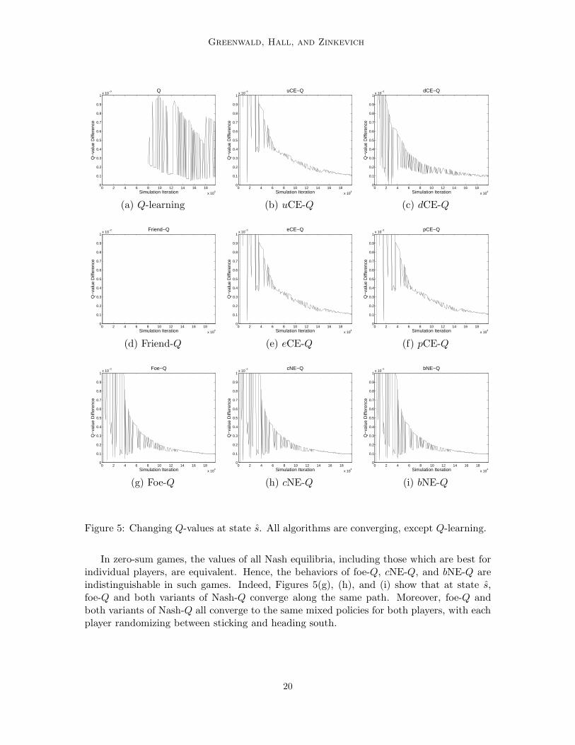
Figure 5: Changing Q-values at state s. All algorithms are converging, except Q-learning.

In zero-sum games, the values of all Nash equilibria, including those which are best forindividual players, are equivalent. Hence, the behaviors of foe-Q, cNE-Q, and bNE-Q areindistinguishable in such games. Indeed, Figures 5(g), (h), and (i) show that at state s,foe-Q and both variants of Nash-Q converge along the same path. Moreover, foe-Q andboth variants of Nash-Q all converge to the same mixed policies for both players, with eachplayer randomizing between sticking and heading south.

20


Soccer Avg. Score Games Convergence? Eqm. Values? Eqm. Play?

Q 0, 0 < 1 No No NoFoe-Q −1.06, 1.06 4170 Yes Yes YesFriend-Q 0.11, −0.11 6115 Yes No No

uCE-Q 2.30, −2.30 4051 Yes Yes YeseCE-Q 1.18, −1.18 4167 Yes Yes YespCE-Q 1.12, −1.12 4104 Yes Yes YescNE-Q 1.86, −1.86 4194 Yes Yes Yes

dCE-Q −0.24, 0.24 4130 Yes Yes YesbNE-Q 0.84, −0.84 4304 Yes Yes Yes

Table 4: Testing phase: Grid soccer played repeatedly, with random start states. Averagescores across 104 moves are shown. The number of games played varied with the agents’policies: sometimes agents moved directly to the goal; other times they digressed. The finalthree columns are analogous to those in Table 3.

Finally, all variants of CE-Q converge. Perhaps surprisingly, all variants of CE-Qconverge to independent minimax equilibrium policies at state s, although in general,correlated-Q can learn correlated equilibrium policies, even in zero-sum Markov games.

5.2 Equilibrium Policies

In Table 4, we present the results of a testing phase for this soccer game. All players, exceptfor Q-learners play a “good” game, meaning that each player wins approximately the samenumber of games; hence, scores are close to 0, 0. Friend-Q tends to let the other player winquickly (observe the large number of games played), and plays a “good” game only becauseof the symmetric nature of grid soccer. All CE-Q and NE-Q variants behave in a mannerthat is similar to one another and similar to foe-Q. Any differences in scores among thesealgorithms is due to randomness in the simulations.

In summary, in grid soccer, a two-player, zero-sum Markov game, Q-learning does notconverge. Intuitively, the rationale for this outcome is clear: Q-learning seeks deterministicoptimal policies, but in this game no such policies exist.9 Friend-Q converges but its policiesare not rational. Correlated-Q learning, however, like Nash-Q learning, learns the same Q-values as foe-Q learning. Nonetheless, correlated-Q learns possibly correlated equilibriumpolicies, while foe-Q and Nash-Q learn minimax equilibrium policies. In the next section,we offer some theoretical justification for our observations about correlated Q-learning.

6. Convergence of Correlated-Q Learning in Two Special Cases

In this section, we discuss two special classes of Markov games: two-player, zero-sum Markovgames and common-interest Markov games. We prove that CE-Q learning behaves like foe-Q learning in the former class of Markov games, and like friend-Q learning in the latter.

9. Recall that in our implementation of Q-learning, players randomize if the action that yields the maximumQ-value is not unique. Nonetheless, at any state in which playing a uniform distribution across suchactions is not an equilibrium policy, Q-learning does not converge.

21


Let Γ = 〈N,A,R〉 denote a one-shot game. Recall from Section 2: N is a set ofn players; A =

∏

i∈N Ai, where Ai is player i’s set of pure actions; and R : A → Rn,

where Ri(a) is player i’s reward at action profile a ∈ A. A mixed strategy profile

(σ1, . . . , σn) ∈ ∆(A1) × . . . × ∆(An) is a profile of randomized actions, one per player.Overloading our notation, we extend R to be defined over mixed strategies:

Ri(σ1, . . . , σn) =∑

a1∈A1

. . .∑

an∈An

σ1(a1) . . . σn(an)Ri(a1, . . . , an) (21)

and, in addition, over correlated policies π ∈ ∆(A): Ri(π) =∑

a∈A π(a)Ri(a). The mixedstrategy profile (σ∗

1 , . . . , σ∗n) is called a Nash equilibrium if σ∗

i is a best-response forplayer i to its opponents’ mixed strategies, for all i ∈ N : i.e.,

Ri(σ∗1 , . . . , σ

∗i , . . . , σ

∗n) = max

σi

Ri(σ∗1 , . . . , σi, . . . σ

∗n) (22)

6.1 Correlated-Q Learning in Two-Player, Zero-Sum Markov Games

Our first result concerns correlated-Q learning in two-player, zero-sum Markov games. Weprove that correlated-Q learns minimax equilibrium Q-values in such games. Hence, theempirical results obtained on the grid soccer game are not surprising.

Let Γ = 〈N,A,R〉 denote a two-player, zero-sum one-shot game. In particular, N ={1, 2}, A = A1 × A2, and Ri : A → R s.t. for all a ∈ A, R1(a) = −R2(a). A mixed

strategy profile (σ∗1 , σ

∗2) ∈ ∆(A1) × ∆(A2) is a minimax equilibrium if:

R1(σ∗1 , σ

∗2) = max

σ1

R1(σ1, σ∗2) (23)

R2(σ∗1 , σ

∗2) = max

σ2

R2(σ∗1 , σ2) (24)

Observe that Nash equilibria and minimax equilibria coincide on zero-sum games.

6.1.1 Convergence

Lemma 9 If Γ is a two-player, zero-sum one-shot game with Nash equilibrium (σ∗1 , σ

∗2),

then

R1(σ∗1 , σ

∗2) ≤ R1(σ

∗1 , σ2), for all σ2 ∈ ∆(A2) (25)

R2(σ∗1 , σ

∗2) ≤ R2(σ1, σ

∗2), for all σ1 ∈ ∆(A1) (26)

Proof Because R1 = −R2, Equation 23 implies:

R2(σ∗1 , σ

∗2) = −R1(σ

∗1 , σ

∗2) = −max

σ1

R1(σ1, σ∗2) = min

σ1

−R1(σ1, σ∗2) = min

σ1

R2(σ1, σ∗2) (27)

so that R2(σ∗1 , σ

∗2) ≤ R2(σ1, σ

∗2), for all σ1 ∈ ∆(A1). The proof for player 1 is analogous.

It is well-known that the value of all Nash equilibria in zero-sum games is unique (vonNeumann and Morgenstern, 1944): i.e., for any Nash equilibria σ and σ′, Ri(σ) = Ri(σ

′),for all i ∈ {1, 2}. In the next theorem, we argue that any correlated equilibrium has theequivalent Nash (or minimax) equilibrium value.

22


Theorem 10 If Γ is a two-player, zero-sum one-shot game with Nash equilibrium (σ∗1 , σ

∗2)

and correlated equilibrium π, then Ri(π) = Ri(σ∗1 , σ

∗2), for all i ∈ {1, 2}.

Proof Consider player 1 and an action a1 ∈ A1 with π(a1) > 0. By Lemma 9, R1(σ∗1 , π(·|a1)) ≥

R1(σ∗1 , σ

∗2). By the definition of correlated equilibrium, R1(a1, π(·|a1)) ≥ R1(σ

∗1 , π(·|a1)).

Hence, R1(a1, π(·|a1)) ≥ R1(σ∗1 , σ

∗2). Because this condition holds for all a1 ∈ A1 with

π(a1) > 0, it follows that R1(π) ≥ R1(σ∗1 , σ

∗2). By an analogous argument, R2(π) ≥

R2(σ∗1 , σ

∗2). Because the game is zero-sum, in fact, R1(π) ≤ R1(σ

∗1 , σ

∗2). Therefore, R1(π) =

R1(σ∗1 , σ

∗2). The argument is analogous for player 2.

Define MMi(R) to be the minimax (equivalently, the Nash) equilibrium value of theith player in a two-player, zero-sum one-shot game Γ. Similarly, define CEi(R) to be the(unique) correlated equilibrium value of the ith player in a two-player, zero-sum one-shotgame Γ. By Theorem 10, CEi(R) = MMi(R).

We say that the zero-sum property holds of the Q-values of a Markov game Γγ attime t if Qt

1(s, a) = −Qt2(s, a), for all s ∈ S and for all a ∈ A(s). In what follows, we show

that multiagent Q-learning preserves the zero-sum property in zero-sum Markov games,provided Q-values are initialized such that this property holds.

Observation 11 Given a two-player, zero-sum one-shot game Γ, any selection π ∈ ∆(A)yields negated values: i.e., R1(π) = −R2(π).

Lemma 12 Multiagent Q-learning preserves the zero-sum property in two-player, zero-sumMarkov games, provided Q-values are initialized such that this property holds.

Proof The proof is by induction on t. By assumption, the zero-sum property holds at timet = 0.

Assume the zero-sum property holds at time t; we show that the property is preservedat time t + 1. In two-player games, multiagent Q-learning updates Q-values as follows:assuming action profile a is played at state s and the game transitions to state s′,

πt+1s′ ∈ f(Qt(s′)) (28)

V t+11 (s′) :=

∑

a′∈A

πt+1s′ (a′)Qt

1(s′, a′) (29)

V t+12 (s′) :=

∑

a′∈A

πt+1s′ (a′)Qt

2(s′, a′) (30)

Qt+11 (s, a) := (1 − α)Qt

1(s, a) + α((1 − γ)R1(s, a) + γV t+11 (s′)) (31)

Qt+12 (s, a) := (1 − α)Qt

2(s, a) + α((1 − γ)R2(s, a) + γV t+12 (s′)) (32)

where f is any selection mechanism. By the induction hypothesis, Qt(s′) is a zero-sumone-shot game. Hence, by Observation 11, V ≡ V t+1

1 (s′) = −V t+12 (s′) ≡ −V , so that the

multiagent-Q learning update procedure simplifies as follows:

Qt+11 (s, a) := (1 − α)Qt

1(s, a) + α((1 − γ)R1(s, a) + γV ) (33)

Qt+12 (s, a) := (1 − α)Qt

2(s, a) + α((1 − γ)R2(s, a) − γV ) (34)

23


Now (i) by the induction hypothesis, Qt1(s, a) = −Qt

2(s, a); (ii) the Markov game is zero-sum: i.e., R1(s, a) = −R2(s, a). Therefore, Qt+1

1 (s, a) = −Qt+12 (s, a): i.e., the zero-sum

property is preserved at time t + 1.

Theorem 13 If all Q-values are initialized such that the zero-sum property holds, thencorrelated-Q learning converges to the minimax equilibrium Q-values in two-player, zero-sum Markov games.

Proof By Lemma 12, correlated-Q learning preserves the zero-sum property: in particular,at time t, Qt

1(s, a) = −Qt2(s, a), for all s ∈ S and for all a ∈ A(s). Thus, correlated-Q

learning simplifies as follows: assuming action profile a is played at state s and the gametransitions to state s′, for all i ∈ {1, 2},

Qt+1i (s, a) := (1 − α)Qt

i(s, a) + α((1 − γ)Ri(s, a) + γCEi(Qt(s′))) (35)

= (1 − α)Qti(s, a) + α((1 − γ)Ri(s, a) + γMMi(Q

t(s′))) (36)

Indeed, the correlated-Q and minimax-Q learning update procedures coincide, so thatcorrelated-Q learning converges to minimax equilibrium Q-values in two-player, zero-sumMarkov games, if all Q-values are initialized such that the zero-sum property holds.

Remark 14 “Correlated value iteration,” that is, synchronous updating of Q-values basedon a correlated equilibrium selection mechanism, also converges to the minimax equilibriumQ-values in two-player, zero-sum Markov games, if all Q-values are initialized such that thezero-sum property holds.

In summary, correlated-Q learning converges in two-player, zero-sum Markov games. Inparticular, correlated-Q learning converges to precisely the minimax equilibrium Q-values.This result applies to both centralized and decentralized versions of the learning algorithm.

6.1.2 Exchangeability

To guarantee that agents play equilibrium policies in a general-sum Markov game, it is notsufficient for agents to learn equilibrium Q-values. In addition, the agents must play anequilibrium at every state that is encountered while playing the game.

Specifically, to guarantee that agents play equilibrium policies in a general-sum Markovgame, the agents must play an equilibrium in each of the one-shot games Q∗(s), where Q∗(s)is the set of Q-values the agents learn at state s ∈ S. In the repeated Bach or Stravinskygame (formulated as a deterministic, Markov game) with γ = 1

2 , egalitarian correlated-Qlearning converges to the Q-values shown in Game 3. Two agents playing Game 3, andmaking independent decisions, can fail to coordinate their behavior, if, say, player 1 selectsand plays her part of the equilibrium (b,B) and player 2 selects and plays his part of theequilibrium (s, S), so that the action profile the agents play is (b, S).

In the special case of two-player, zero-sum Markov games, however, it suffices for agentsto learn minimax equilibrium Q-values, because miscoordination in two-player, zero-sum

24


Game 3: Repeated Bach or Stravinsky Q-values for γ = 12

B Sb 7

4 , 54

34 , 3

4s 3

4 , 34

54 , 7

4

one-shot games is ruled out by the exchangeability property. The exchangeability propertyholds in a one-shot game if, assuming each player i selects a correlated equilibrium πi

and plays his marginal distribution, call it πAi, the mixed strategy profile (πAi

)i∈I is aNash equilibrium. Our proof that the exchangeability property holds (for the correlatedequilibrium solution concept) in two-player, zero-sum one-shot games relies on the fact thatexchangeability also holds of Nash equilibria in this class of games:

Lemma 15 If Γ is a two-player, zero-sum one-shot game with Nash equilibria σ and σ′,then (σ1, σ

′2) is a Nash equilibrium.

Proof Since the minimax equilibrium value of a zero-sum game is unique, R1(σ) = R1(σ′).

Observe that R1(σ1, σ2) ≤ R1(σ1, σ′2), by Lemma 9 (Equation 25), and R1(σ1, σ

′2) ≤

R1(σ′1, σ

′2), by the definition of minimax equilibrium (Equation 23). Hence, R1(σ1, σ2) =

R1(σ1, σ′2) = R1(σ

′1, σ

′2). Because R1 = −R2, it follows that R2(σ1, σ2) = R2(σ1, σ

′2) =

R2(σ′1, σ

′2). Now R2(σ1, σ

′2) = R2(σ1, σ2) = maxσ′′

2R2(σ1, σ

′′2 ) and R1(σ1, σ

′2) = R1(σ1, σ2) =

maxσ′′

1R1(σ

′′1 , σ2). Therefore, (σ1, σ

′2) is a Nash equilibrium.

Define πAito be the marginal distribution of π over Ai: i.e.,

πAi(ai) =

∑

a−i∈A−i

π(a−i, ai) (37)

Definition 16 A one-shot game Γ satisfies the exchangeability property if for any set ofn correlated equilibria π1, π2,. . . ,πn, it is the case that (π1

A1, . . . , πn

An) is a Nash equilibrium.

Theorem 17 The exchangeability property holds in two-player, zero-sum one-shot games.

Proof By Lemma 15, it suffices to show that for any correlated equilibrium π, (πA1, πA2

)is a Nash equilibrium. The proof of this statement relies on a series of lemmas.

Lemma 18 In a two-player, zero-sum one-shot game Γ, if π is a correlated equilibrium,then maxa′

1R1(a

′1, π(· | a1)) = MM1(R), for all a1 ∈ A1 such that πA1

(a1) > 0.

Proof By the definition of correlated equilibrium, for all a1 ∈ A1 such that πA1(a1) > 0,

a1 is a best-response to π(· | a1): i.e., R1(a1, π(·|a1)) ≥ R1(a′1, π(·|a1)), for all a′1 ∈ A1. By

Theorem 10, R1(π) = MM1(R). Therefore, maxa′

1∈A1

R1(a′1, π(·|a1)) = R1(a1, π(·|a1)) =

MM1(R), for all such a1 ∈ A1 such that πA1(a1) > 0.

25


Corollary 19 In a two-player, zero-sum one-shot game Γ, if π is a correlated equilibrium,then maxσ1

R1(σ1, π(· | a1)) = MM1(R), for all a1 ∈ A1 such that πA1(a1) > 0.

Lemma 20 In a two-player, zero-sum one-shot game Γ, if (σ1, σ2) is a Nash equilibrium,then (σ1, σ

′2) is also a Nash equilibrium, for any σ′

2 such that maxσ′

1R1(σ

′1, σ

′2) = MM1(R).

Proof By assumption, R1(σ1, σ2) = MM1(R). By Lemma 9 (Equation 25), R1(σ1, σ′2) ≥

MM1(R). But R1(σ′1, σ

′2) ≤ MM1(R), for all σ′

1 ∈ ∆(A1). Hence, R1(σ1, σ′2) = MM1(R),

which implies (i) σ1 is a best-response to σ′2, and (ii) σ′

2 is a best-response to σ1, sinceR2(σ1, σ

′2) = −R1(σ1, σ

′2) = −MM1(R) = MM2(R) and R2(σ1, σ2) = MM2(R).

Lemma 21 In a two-player, zero-sum one-shot game Γ, for any λ ∈ [0, 1] and for any twoNash equilibria σ and σ′, if σ′′

2 = λσ2 + (1 − λ)σ′2, then (σ1, σ

′′2 ) is a Nash equilibrium.

Proof By Lemma 15, σ1 is a best response to σ′′2 :

R1(σ1, σ′′2 ) = λR1(σ1, σ2) + (1 − λ)R1(σ1, σ

′2) (38)

= λ

(

maxσ′′

1

R1(σ′′1 , σ2)

)

+ (1 − λ)

(

maxσ′′

1

R1(σ′′1 , σ′

2)

)

(39)

≥ maxσ′′

1

R1(σ′′1 , λσ2 + (1 − λ)σ′

2) (40)

= maxσ′′

1

R1(σ′′1 , σ′′

2 ) (41)

Equation 40 follow from the following fact: for any f, g : X → R and for any a, b ∈ R,maxx∈X(af(x) + bg(x)) ≤ a(maxx∈X f(x)) + b(maxy∈X g(y)).

By Lemma 15, σ′′2 is a best response to σ1:

R2(σ1, σ′′2 ) = λR2(σ1, σ2) + (1 − λ)R2(σ1, σ

′2) (42)

= λ

(

maxσ′′′

2

R2(σ1, σ′′′2 )

)

+ (1 − λ)

(

maxσ′′′

2

R2(σ1, σ′′′2 )

)

(43)

= maxσ′′′

2

R2(σ1, σ′′′2 ) (44)

Therefore, (σ1, σ′′2 ) is a Nash equilibrium.

By Corollary 19, player 1 achieves his minimax payoff whenever he plays a best-response toπ(· | a1), for all a1 ∈ A1 such that πA1

(a1) > 0. By Lemma 20, π(· | a1) is player 2’s partof a Nash equilibrium, and by repeated application of Lemma 21, any convex combinationof π(· | a1)’s, is player 2’s part of a Nash equilibrium, for all such a1 ∈ A1.

In particular, πA2is player 2’s part of a Nash equilibrium, since

πA2(a2) =

∑

a1∈A1

π(a1, a2) (45)

=∑

{a1∈A1|π(a1)>0}

π(a2 | a1)π(a1) (46)

26


implying

πA2=

∑

{a1∈A1|π(a1)>0}

π(· | a1)π(a1) (47)

Analogously, one can show that πA1is player 1’s part of a Nash equilibrium. Therefore, by

Lemma 15, (πA1, πA2

) is a Nash equilibrium.

6.2 Correlated-Q Learning in Common-Interest Markov Games

In a common-interest one-shot game Γ, for all i, j ∈ N and for all a ∈ A, it is the casethat Ri(a) = Rj(a). More generally, in a common-interest Markov game Γγ , the one-shotgame defined at each state is common-interest: i.e., for all i, j ∈ N , for all s ∈ S, and forall a ∈ A(s), it is the case that Ri(s, a) = Rj(s, a).

We say that the common-interest property holds of the Q-values of a Markov gameat time t if Qt

i(s, a) = Qtj(s, a), for all i, j ∈ N , for all s ∈ S, and for all a ∈ A(s). In

what follows, we show that multiagent Q-learning preserves the common-interest propertyin common-interest Markov games, if Q-values are initialized such that this property holds.

Observation 22 Given a common-interest one-shot game Γ, any selection π ∈ ∆(A) yieldscommon values: i.e., Ri(π) = Rj(π), for all i, j ∈ N .

Lemma 23 Multiagent Q-learning preserves the common-interest property in common-interest Markov games, provided Q-values are initialized such that this property holds.

Proof The proof is by induction on t. By assumption, the common-interest property holdsat time t = 0.

Assume the common-interest property holds at time t; we show that this property ispreserved at time t+1. Multiagent Q-learning updates Q-values as follows: assuming actionprofile a is played at state s and the game transitions to state s′,

πt+1s′ ∈ f(Qt(s′)) (48)

V t+1i (s′) :=

∑

a′∈A

πt+1s′ (a′)Qt

i(s′, a′) (49)

Qt+1i (s, a) := (1 − α)Qt

i(s, a) + α((1 − γ)Ri(s, a) + γV t+1i (s′)) (50)

where f is any selection mechanism. By the induction hypothesis, Qt(s′) is a common-interest one-shot game. Hence, by Observation 22, V t+1

i (s′) = V t+1j (s′) ≡ V , for all i, j ∈ N ,

so that the multiagent-Q learning update procedure simplifies as follows:

Qt+1i (s, a) := (1 − α)Qt

i(s, a) + α((1 − γ)Ri(s, a) + γV ) (51)

Now, for all i, j ∈ N , (i) by the induction hypothesis, Qti(s, a) = Qt

j(s, a); (ii) the Markov

game is common-interest: i.e., Ri(s, a) = Rj(s, a). Therefore, Qt+1i (s, a) = Qt+1

j (s, a), forall i, j ∈ N : i.e., the common-interest property is preserved at time t + 1.

27


Given a one-shot game, an equilibrium π∗ is called Pareto-optimal if there does notexist another equilibrium π such that (i) for all i ∈ N , Ri(π) ≥ Ri(π

∗), and (ii) there existsi ∈ N such that Ri(π) > Ri(π

∗).

Observation 24 In a common-interest one-shot game Γ, for any equilibrium π ∈ ∆(A)that is Pareto-optimal, Ri(π) = maxa∈A Ri(a), for all i ∈ N .

Theorem 25 If all Q-values are initialized such that the common-interest property holds,then any multiagent Q-learning algorithm that selects Pareto-optimal equilibria convergesto friend Q-values in common-interest Markov games.

Proof By Lemma 23, the common-interest property is preserved by correlated-Q learning:in particular, at time t, Qt

i(s, a) = Qtj(s, a), for all i, j ∈ N , for all s ∈ S, and for all

a ∈ A(s). By Observation 24, any multiagent-Q learning update procedure with a Pareto-optimal selection mechanism simplifies as follows: for all i ∈ N ,

Qt+1i (s, a) := (1 − α)Qt

i(s, a) + α((1 − γ)Ri(s, a) + γ maxa′∈A(s′)

Qti(s

′, a′)) (52)

assuming action profile a is played at state s and the game transitions to state s′. Indeed,the correlated-Q and friend-Q learning update procedures coincide, so that correlated-Qlearning converges to friend Q-values in common-interest Markov games, if all Q-values areinitialized such that the common-interest property holds.

The following corollary follows immediately, since friend-Q learning converges to Pareto-optimal equilibrium Q-values in common-interest Markov games (Littman, 2001).

Corollary 26 If all Q-values are initialized such that the common-interest property holds,then any multiagent Q-learning algorithm that selects Pareto-optimal equilibria convergesto Pareto-optimal equilibrium Q-values in common-interest Markov games.

The multiagent Q-learning algorithms uCE-Q, eCE-Q, pCE-Q, dCE-Q, and bNE-Q allrely on Pareto-optimal equilibrium selection operators, and thus converge to Pareto-optimalequilibrium Q-values in common-interest Markov games, provided Q-values are initializedsuch that the common-interest property holds.

Observe that an arbitrary CE-Q learner need not learn Q-values that correspond toPareto-optimal equilibrium policies in common-interest Markov games, because an arbitraryCE-Q operator need not select Pareto-optimal equilibria. Similarly, cNE-Q need not selectsuch equilibria nor learn such Q-values.

7. Related Work

While Markov games have been the subject of extensive research since the latter part ofthe twentieth century, multiagent reinforcement learning in Markov games has only recentlyreceived attention. In 1994, the field was launched with Littman’s (1994) seminal paper onminimax Q-learning. The proof of convergence of this algorithm to a minimax equilibrium

28


policy appeared subsequently in Littman and Szepesvari (1996). This algorithm computesthe value of a state as the value to one player of the zero-sum game induced by the Q-valuesat that state. Later, Q-learning techniques were extended to general-sum games by Hu andWellman (2003). Here, each state’s value is computed based an arbitrary Nash equilibriumof the matrix game induced by the Q-values at that state. This algorithm has weak conver-gence guarantees (e.g., Bowling (2000)). Moreover, the computation of a Nash equilibrium,even for a bimatrix game, is in and of itself a hard problem (e.g., Papadimitriou (2001)).Finally, algorithms have also been designed for the special case of coordination games. Forexample, Littman’s (2001) friend-Q algorithm converges to equilibrium policies in this classof games. In addition, Claus and Boutilier (1998), generalize the classic game-theoreticlearning method known as fictitious play (e.g., Robinson (1951)) to multiagent reinforce-ment learning, and apply their algorithm to this class of games. In addition to Q-learningalgorithms, there are also model-based techniques like R-max (Brafman and Tennenholtz,2001), which has been proven to learn near-minimax equilibrium policies in finite, average-reward, zero-sum Markov games; and policy-search techniques like WoLF (Bowling andVeloso, 2002), which is based on a variable learning rate.

To summarize, multiagent reinforcment learning in general-sum Markov games is anopen problem: no algorithms exist to date that are guaranteed to learn an equilibriumpolicy of any type in arbitrary general-sum Markov games.

8. Conclusion

This research originates with a proof of the existence of stationary correlated equilibriumpolicies in finite, discounted, general-sum Markov games (Greenwald and Zinkevich, 2005),which motivates the design of a class of multiagent Q-learning algorithms we call correlatedQ-learning. Theoretically, we established that correlated-Q learning converges to station-ary correlated equilibrium policies in two special classes of Markov games, namely zero-sumand common-interest. Empirically, we established that correlated-Q learning converges tostationary correlated equilibrium policies on a standard test bed of Markov games. Ourempirical findings suggest that like Nash-Q, correlated Q-learning can serve an effectiveheuristic for the computation of equilibrium policies in general-sum Markov games. How-ever, correlated-Q learning is more efficient than Nash-Q learning.

In past work, we have studied adaptive algorithms for learning game-theoretic equilibriain repeated games (Greenwald and Jafari, 2003). In ongoing work, we are combining theseadaptive algorithms with multiagent Q-learning. Specifically, we are replacing the linearprogramming call in CE-Q learning with an adaptive procedure that converges to the setof correlated equilibria (e.g., Foster and Vohra (1997)). Similarly, we are studying anadaptive version of minimax-Q by replacing its linear programming call with an adaptiveprocedure that converges to minimax equilibrium (e.g., Freund and Schapire (1996)). (Noadaptive algorithm is known to converge to Nash equilibrium.) This adaptive approachcould simultaneously achieve an objective of artificial intelligence researchers—to learn Q-values—and an objective of game theory researchers—to learn game-theoretic equilibria.

Practically speaking, one of the goals of this line of research is to improve the design andimplementation of multiagent systems. At one extreme, multiagent system designers act ascentral planners, equipping all agents in the system with specified behaviors; however, such

29


systems are rarely compatible with agents’ incentives. At the other extreme, multiagentsystem designers allow the agents to specify their own behavior; however, these systemsare susceptible to miscoordination. A multiagent system design based on the correlatedequilibrium solution concept would perhaps rely on a central planner (i.e., the referee),but nonetheless, would specify rational agent behavior. Such a design would not onlyfacilitate multiagent coordination, but could generate greater rewards to the agents thanany multiagent system design based on the Nash equilibrium solution concept.

Acknowledgments

The authors are grateful to Michael Littman for inspiring discussions. We also thank DinahRosenberg and Roberto Serrano for comments on an earlier draft of this paper. This researchwas supported by NSF Career Grant #IIS-0133689.

References

R. Aumann. Subjectivity and correlation in randomized strategies. Journal of MathematicalEconomics, 1:67–96, 1974.

R. Bellman. Dynamic Programming. Princeton University Press, New Jersey, 1957.

M. Bowling. Convergence problems of general-sum multiagent reinforcement learning. InProceedings of the Seventeenth International Conference on Machine Learning, pages 89–94. Morgan Kaufman, 2000.

Michael Bowling and Manuela Veloso. Multiagent learning using a variable learning rate.Artificial Intelligence, 136:215–250, 2002.

Ronen I. Brafman and Moshe Tennenholtz. R-MAX — a general polynomial time algorithmfor near-optimal reinforcement learning. In IJCAI, pages 953–958, 2001.

C. Claus and C. Boutilier. The dynamics of reinforcement learning in cooperative multi-agent systems. In Proceedings of the Fifteenth National Conference on Artificial Intelli-gence, pages 746–752, June 1998.

Vincent Conitzer and Tuomas Sandholm. Complexity results about Nash equilibria. InProceedings of the Eighteenth International Joint Conference on Artificial Intelligence,pages 765–771, August 2003.

D. Foster and R. Vohra. Regret in the on-line decision problem. Games and EconomicBehavior, 21:40–55, 1997.

Y. Freund and R. Schapire. Game theory, on-line prediction, and boosting. In Proceedingsof the 9th Annual Conference on Computational Learning Theory, pages 325–332. ACMPress, May 1996.

Itzhak Gilboa and Eitan Zemel. Nash and correlated equilibria: Some complexity consid-erations. Games and Economic Behavior, 1:80–93, 1989.

30


A. Greenwald and K. Hall. Correlated Q-learning. In Proceedings of the Twentieth Inter-national Conference on Machine Learning, pages 242–249, 2003.

A. Greenwald and A. Jafari. A general class of no-regret algorithms and game-theoreticequilibria. In Proceedings of the 2003 Computational Learning Theory Conference, pages1–11, August 2003.

A. Greenwald and M. Zinkevich. A direct proof of the existence of correlated equilibriumpolicies in general-sum markov games. Technical Report 7, Brown University, Departmentof Computer Science, June 2005.

J. Hu and M. Wellman. Nash Q-learning for general-sum stochastic games. MachineLearning Research, 4:1039–1069, 2003.

M. Littman. Markov games as a framework for multi-agent reinforcement learning. InProceedings of the Eleventh International Conference on Machine Learning, pages 157–163, July 1994.

M. Littman. Friend or foe Q-learning in general-sum Markov games. In Proceedings ofEighteenth International Conference on Machine Learning, pages 322–328, June 2001.

M. Littman and C. Szepesvari. A generalized reinforcement learning model: Convergenceand applications. In Proceedings of the Thirteenth International Conference on MachineLearning, pages 310–318, 1996.

J. Nash. Non-cooperative games. Annals of Mathematics, 54:286–295, 1951.

M. Osborne and A. Rubinstein. A Course in Game Theory. MIT Press, Cambridge, 1994.

C. Papadimitriou. Algorithms, games, and the internet. In Proceedings on 33rd AnnualACM Symposium on Theory of Computing, 2001.

M.L. Puterman. Markov Decision Processes: Discrete Stochastic Dynamic Programming.Wiley-Interscience, 1994.

J. Robinson. An iterative method of solving a game. Annals of Mathematics, 54:298–301,1951.

L.S. Shapley. A value for n-person games. In H. Kuhn and A.W. Tucker, editors, Contri-butions to the Theory of Games, volume II, pages 307–317. Princeton University Press,1953.

K. Shell. General equilibrium: The new palgrave. In J. Eatwell, M. Milgate, and P. Newman,editors, Sunspot Equilibrium, pages 274–280. Macmillan, New York, 1989.

R. Sutton and A. Barto. Reinforcement Learning: An Introduction. MIT Press, Mas-sachusetts, 1998.

J. von Neumann and O. Morgenstern. The Theory of Games and Economic Behavior.Princeton University Press, Princeton, 1944.

C. Watkins. Learning from Delayed Rewards. PhD thesis, Cambridge University, Cambridge,1989.

31

Documents

Correlated Q-Learning Amy Greenwald, Keith Hall …cs.brown.edu/research/pubs/pdfs/2005/Greenwald-2005-CL.pdfCorrelated Q-Learning Amy Greenwald, Keith Hall and Martin Zinkevich Department