Embed Size (px)
Citation preview
Coordinate Systems and Transformations
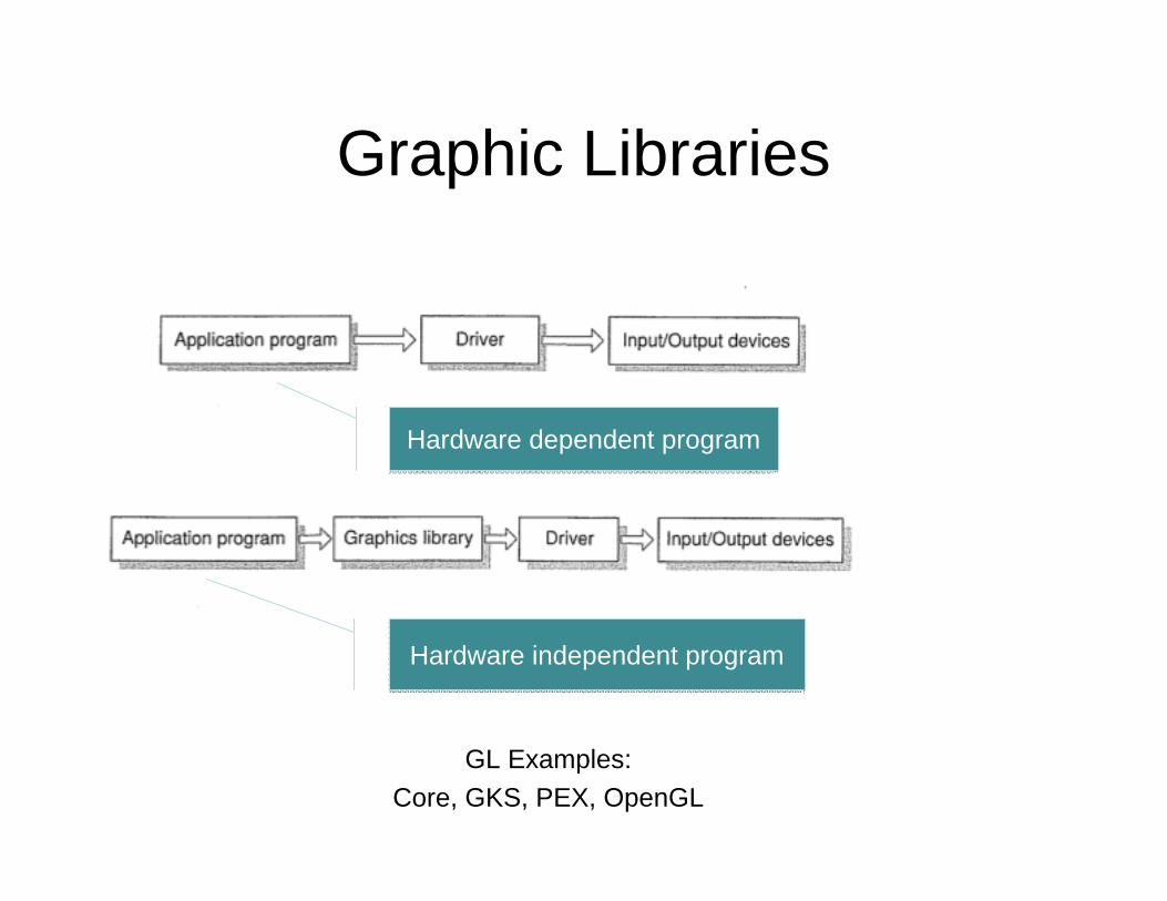
Graphic Libraries
Hardware dependent programHardware dependent program
Hardware independent programHardware independent program
GL Examples:Core, GKS, PEX, OpenGL
Coordinate Systems
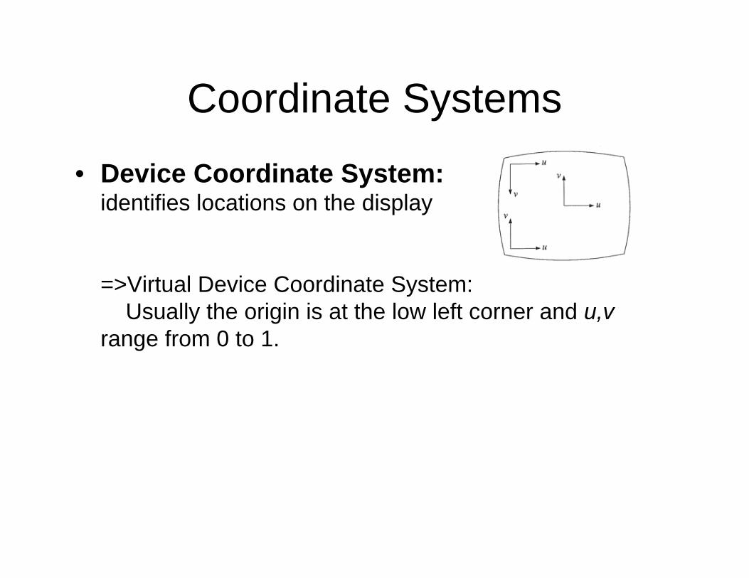
• Device Coordinate System: identifies locations on the display
=>Virtual Device Coordinate System:Usually the origin is at the low left corner and u,v
range from 0 to 1.
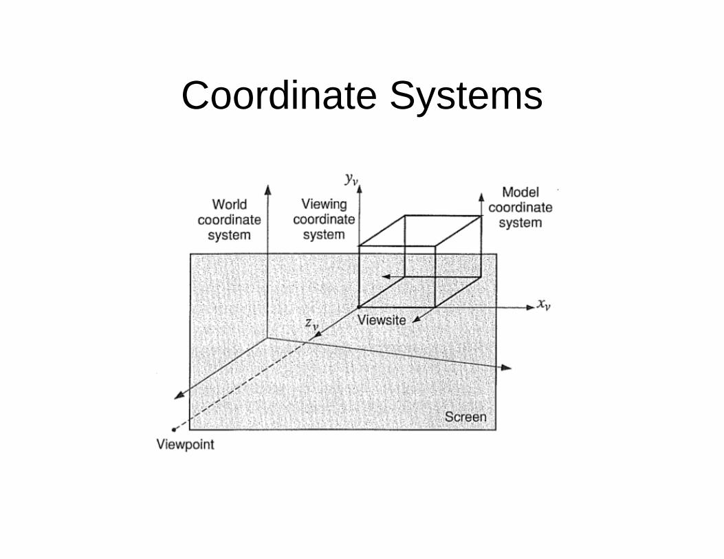
Coordinate Systems
• Model Coordinate System(MCS): identifies the shapes of object and it is attached to the object. Therefore the MCS moves with the object in the WCS
• World Coordinate System (WCS): identifies locations of objects in the world in the application.
• Viewing Coordinate System (VCS): Defined by the viewpoint and viewsite
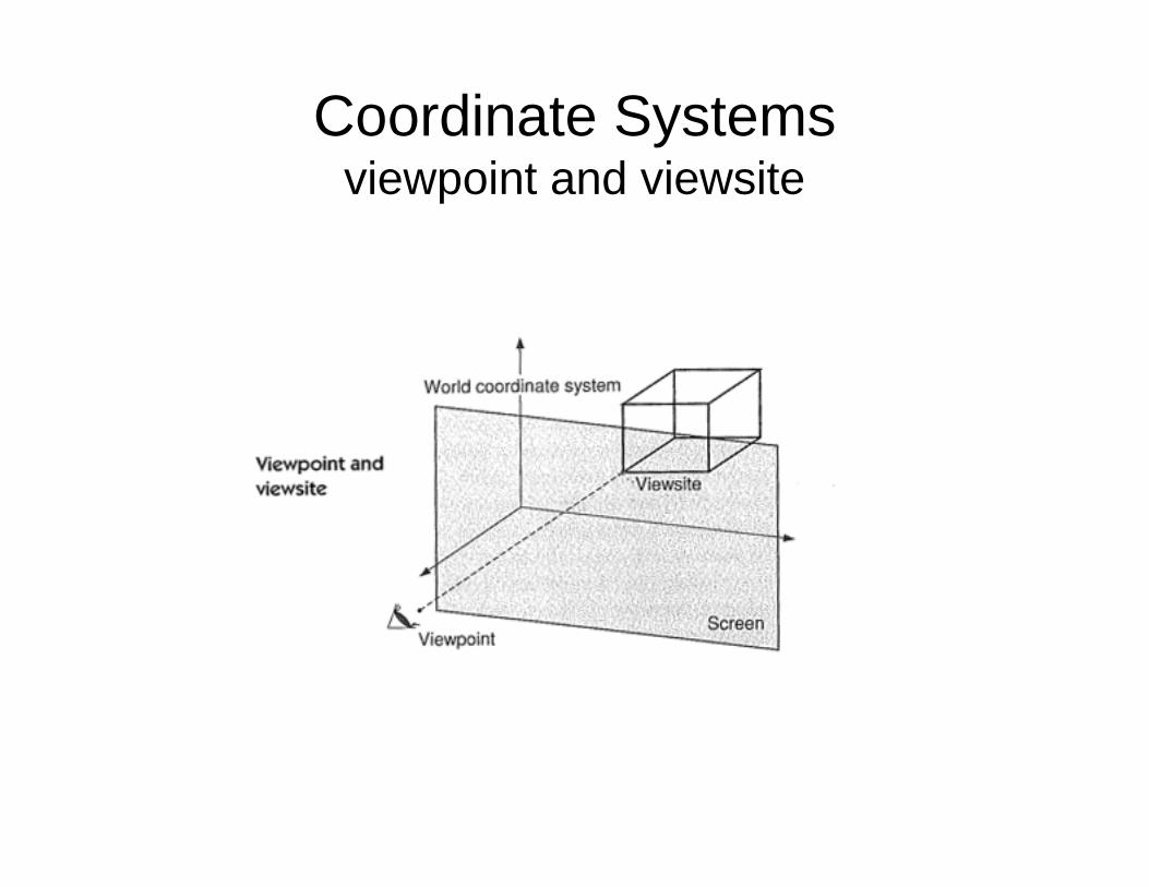
Coordinate Systemsviewpoint and viewsite
Coordinate Systems
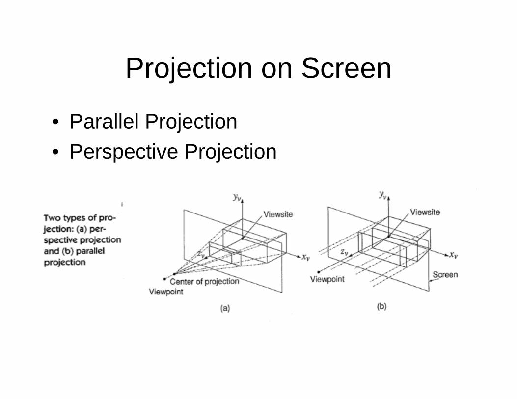
Projection on Screen
• Parallel Projection• Perspective Projection
Parallel Projection
• Preserve actual dimensions and shapes of objects
• Preserve parallelism
• Angles preserved only on faces parallel to the projection plane
• Orthographic projection is one type of parallel projection
Perspective Projection
• Doesn’t preserve parallelism
• Doesn’t preserve actual dimensions and angles of objects, therefore shapes deformed
• Popular in art (classic painting); architectural design and civil engineering.
• Not commonly used in mechanical engineering
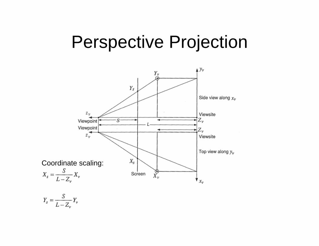
Perspective Projection
Coordinate scaling:
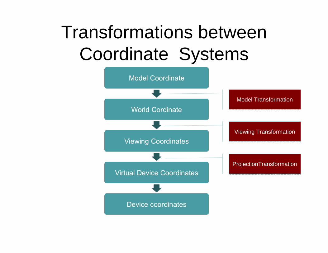
Transformations between Coordinate Systems
Model TransformationModel Transformation
Viewing TransformationViewing Transformation
ProjectionTransformationProjectionTransformation
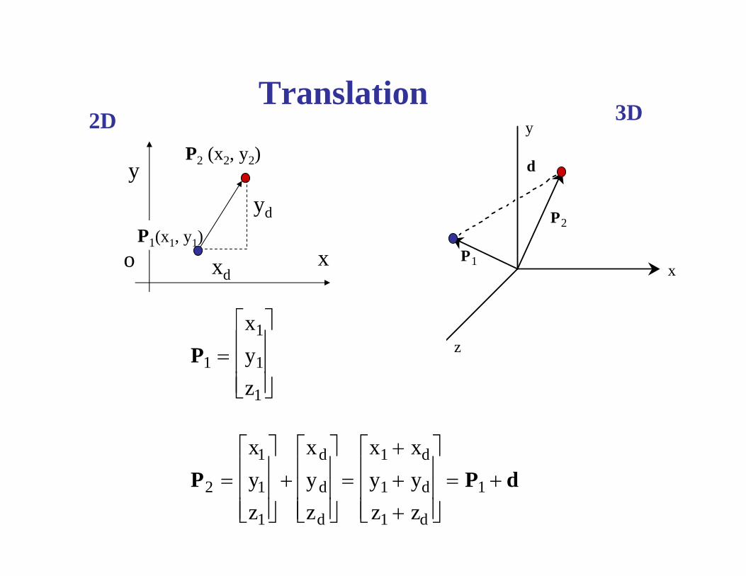
Translation
P2 (x2, y2)
x
y
P1(x1, y1)o xd
yd P2
P1
y
x
z
d
P1 =x1
y1
z1
⎡
⎣
⎢ ⎢ ⎢
⎤
⎦
⎥ ⎥ ⎥
P2 =x1
y1
z1
⎡
⎣
⎢ ⎢ ⎢
⎤
⎦
⎥ ⎥ ⎥
+xd
yd
zd
⎡
⎣
⎢ ⎢ ⎢
⎤
⎦
⎥ ⎥ ⎥
=x1 + xd
y1 + yd
z1 + zd
⎡
⎣
⎢ ⎢ ⎢
⎤
⎦
⎥ ⎥ ⎥
= P1 + d
3D2D
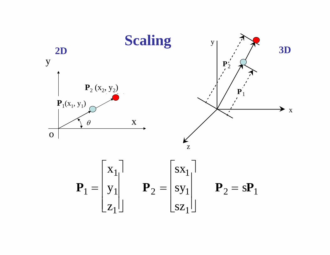
Scaling y
x
z
P2
P1
3D
P1 =x1
y1
z1
⎡
⎣
⎢ ⎢ ⎢
⎤
⎦
⎥ ⎥ ⎥ P2 =
sx1
sy1
sz1
⎡
⎣
⎢ ⎢ ⎢
⎤
⎦
⎥ ⎥ ⎥ P2 = sP1
y
V(x, y)
V’(x’, y’)
θ xo
2D
P2 (x2, y2)
P1(x1, y1)
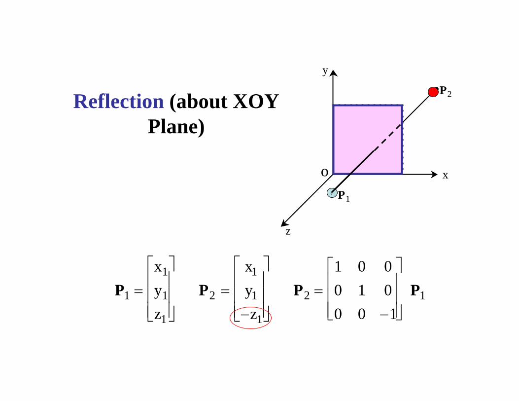
Reflection (about XOY Plane)
y
x
z
P2
P1
P1 =x1
y1
z1
⎡
⎣
⎢ ⎢ ⎢
⎤
⎦
⎥ ⎥ ⎥ P2 =
x1
y1
−z1
⎡
⎣
⎢ ⎢ ⎢
⎤
⎦
⎥ ⎥ ⎥ P2 =
1 0 00 1 00 0 −1
⎡
⎣
⎢ ⎢ ⎢
⎤
⎦
⎥ ⎥ ⎥
P1
o
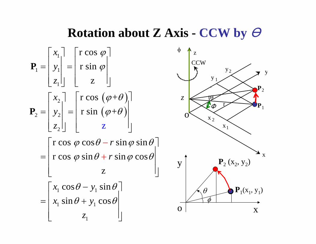
Rotation about Z Axis - CCW by Ө
( )( )
1
1 1
1
2
2 2
2
1 1
1 1
1
r cos r sin
z
r cos +r sin +
r cos cos sin sinr cos sin sin cos
z
cos sin sin cos
z
xyz
xyz
rr
x yx y
z
ϕϕ
ϕ θϕ θ
ϕ θ ϕ θϕ θ ϕ θ
θ θθ θ
⎡ ⎤ ⎡ ⎤⎢ ⎥ ⎢ ⎥= =⎢ ⎥ ⎢ ⎥⎢ ⎥ ⎢ ⎥⎣ ⎦ ⎣ ⎦
⎡ ⎤⎡ ⎤⎢ ⎥⎢ ⎥= = ⎢ ⎥⎢ ⎥⎢ ⎥⎢ ⎥⎣ ⎦ ⎣ ⎦
⎡ ⎤−+⎢ ⎥= ⎢ ⎥
⎢ ⎥⎣ ⎦−⎡ ⎤
⎢ ⎥= +⎢ ⎥⎢ ⎥⎣ ⎦
P
P
x
y
θφ
o
P1(x1, y1)
φ z
y
x
θr
P2
P1
1x2x
1y2y
CCW
Φz
P2 (x2, y2)
o
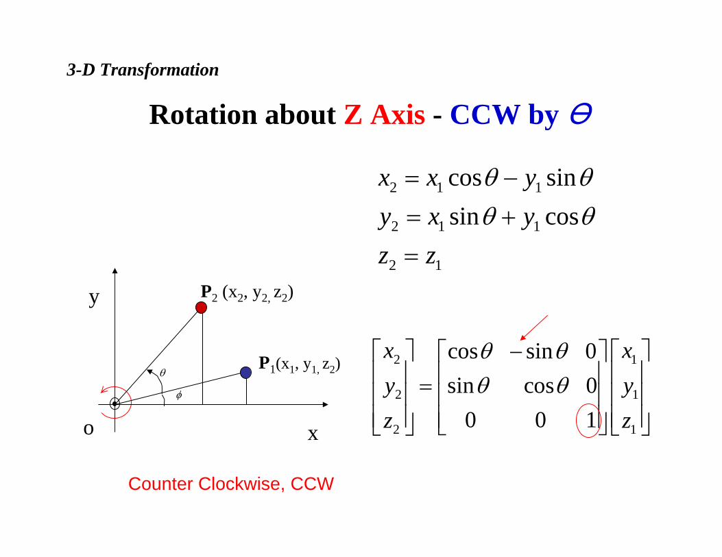
3-D Transformation
x
y
θ
φ
o
2 1 1
2 1 1
2 1
cos sinsin cos
x x yy x yz z
θ θθ θ
= −= +=
2 1
2 1
2 1
cos sin 0sin cos 0
0 0 1
x xy yz z
θ θθ θ
−⎡ ⎤ ⎡ ⎤⎡ ⎤⎢ ⎥ ⎢ ⎥⎢ ⎥=⎢ ⎥ ⎢ ⎥⎢ ⎥⎢ ⎥ ⎢ ⎥⎢ ⎥⎣ ⎦⎣ ⎦ ⎣ ⎦
P1(x1, y1, z2)
P2 (x2, y2, z2)
Rotation about Z Axis - CCW by Ө
Counter Clockwise, CCW
y
z
θ
φ
o
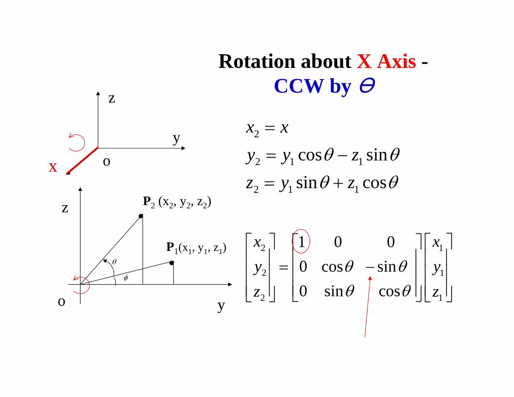
Rotation about X Axis -CCW by Ө
y
z
x o
2
2 1 1
2 1 1
cos sinsin cos
x xy y zz y z
θ θθ θ
== −= +
2 1
2 1
2 1
1 0 00 cos sin0 sin cos
x xy yz z
θ θθ θ
⎡ ⎤ ⎡ ⎤⎡ ⎤⎢ ⎥ ⎢ ⎥⎢ ⎥= −⎢ ⎥ ⎢ ⎥⎢ ⎥⎢ ⎥ ⎢ ⎥⎢ ⎥⎣ ⎦⎣ ⎦ ⎣ ⎦
P1(x1, y1, z1)
P2 (x2, y2, z2)
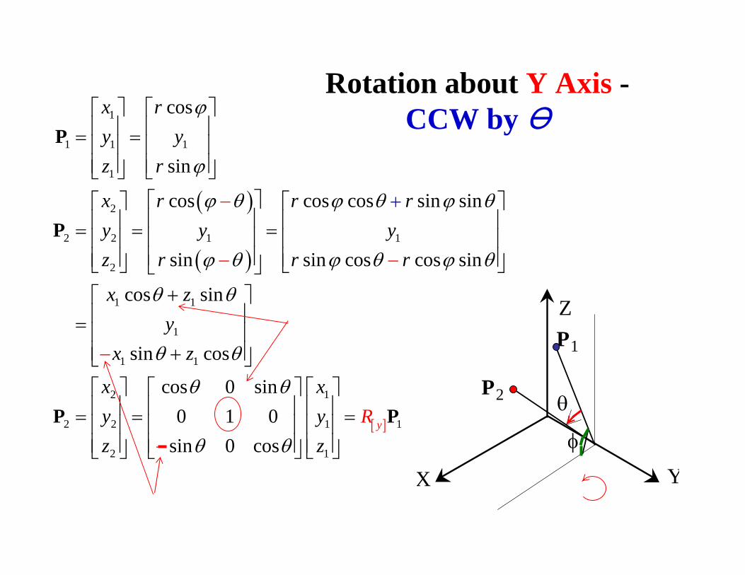
Rotation about Y Axis -CCW by Ө
Z
X Y
φ
θP2
P1
( )
( )
1
1 1 1
1
2
2 2 1 1
2
1 1
1
1 1
2
2
cos
sin
cos cos cos sin sin
sin sin cos cos sin
cos sin
sin cos
x ry yz r
x r r ry y yz r r r
x zy
x z
x
ϕ
ϕ
ϕ θ ϕ θ ϕ θ
ϕ θ ϕ θ ϕ θ
θ θ
θ θ
⎡ ⎤ ⎡ ⎤⎢ ⎥ ⎢ ⎥= =⎢ ⎥ ⎢ ⎥⎢ ⎥ ⎢ ⎥⎣ ⎦ ⎣ ⎦
⎡ ⎤⎡ ⎤ ⎡ ⎤⎢ ⎥⎢ ⎥ ⎢ ⎥= = =⎢ ⎥⎢ ⎥ ⎢ ⎥⎢ ⎥⎢ ⎥ ⎢ ⎥⎣ ⎦ ⎣ ⎦⎣ ⎦
+⎡ ⎤⎢ ⎥= ⎢ ⎥⎢ ⎥+⎣
+
⎦
−
−
=
−
−
P
P
P [ ]
1
2 1 1
2 1
cos 0 sin0 1 0
sin 0 cosyR
xy yz z
θ θ
θ θ
⎡ ⎤ ⎡ ⎤ ⎡ ⎤⎢ ⎥ ⎢ ⎥ ⎢ ⎥= =⎢ ⎥ ⎢ ⎥ ⎢ ⎥⎢ ⎥ ⎢ ⎥ ⎢ ⎥⎣ ⎦ ⎣ ⎦ ⎣ ⎦−
P
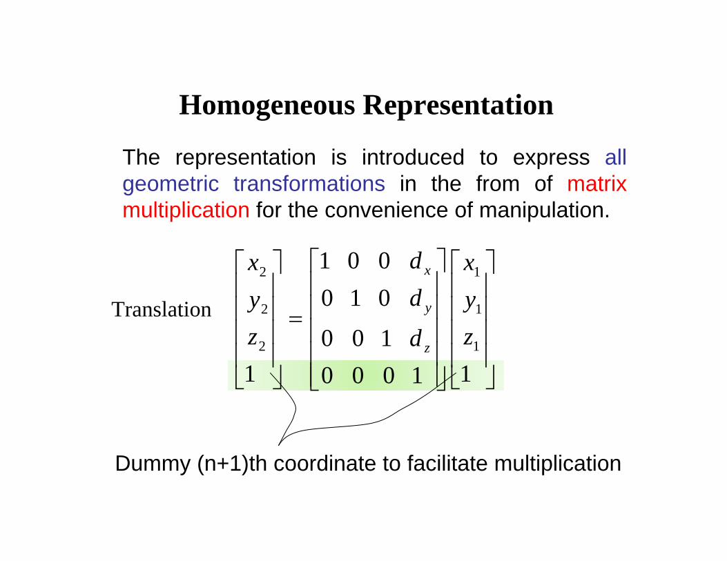
Homogeneous Representation
The representation is introduced to express all geometric transformations in the from of matrix multiplication for the convenience of manipulation.
Dummy (n+1)th coordinate to facilitate multiplication
2 1
2 1
2 1
1 0 00 1 0
0 0 11 10 0 0 1
x
y
z
dx xdy y
z zd
⎡ ⎤⎡ ⎤ ⎡ ⎤⎢ ⎥⎢ ⎥ ⎢ ⎥⎢ ⎥⎢ ⎥ ⎢ ⎥=⎢ ⎥⎢ ⎥ ⎢ ⎥⎢ ⎥⎢ ⎥ ⎢ ⎥⎢ ⎥⎣ ⎦ ⎣ ⎦⎣ ⎦
Translation
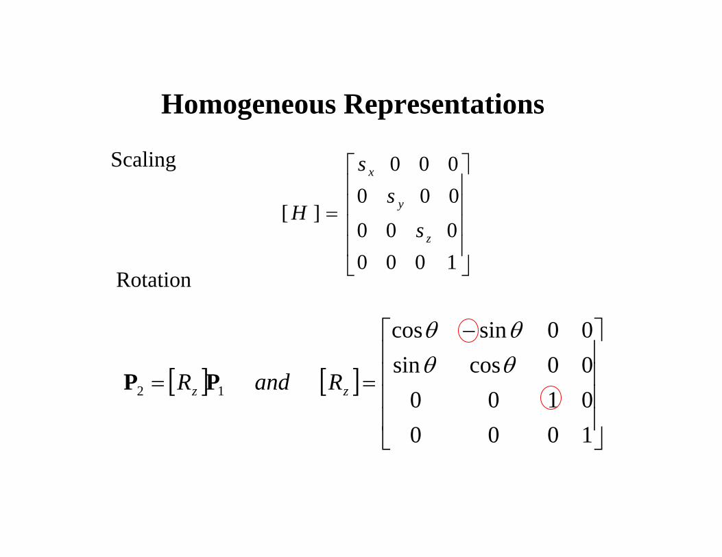
Homogeneous Representations
⎥⎥⎥⎥
⎦
⎤
⎢⎢⎢⎢
⎣
⎡
=
1000000000000
][z
y
x
ss
s
H
Scaling
Rotation
[ ] [ ]⎥⎥⎥⎥
⎦
⎤
⎢⎢⎢⎢
⎣
⎡ −
==
1000010000cossin00sincos
12
θθθθ
zz RandR PP

Homogeneous Representations
[ ] [ ]⎥⎥⎥⎥
⎦
⎤
⎢⎢⎢⎢
⎣
⎡
±±
±
==
1000010000100001
12 MandM PP
[ ]
1 0 0 0 cos 0 sin 00 cos sin 0 0 1 0 0
; 0 sin cos 0 sin 0 cos 00 0 0 1 0 0 0 1
x yR R
θ θθ θθ θ θ θ
⎡ ⎤ ⎡ ⎤⎢ ⎥ ⎢ ⎥−⎢ ⎥ ⎢ ⎥⎡ ⎤= =⎣ ⎦⎢ ⎥ ⎢ ⎥⎢ ⎢
⎦ ⎣ ⎦
−⎥ ⎥
⎣
Reflection
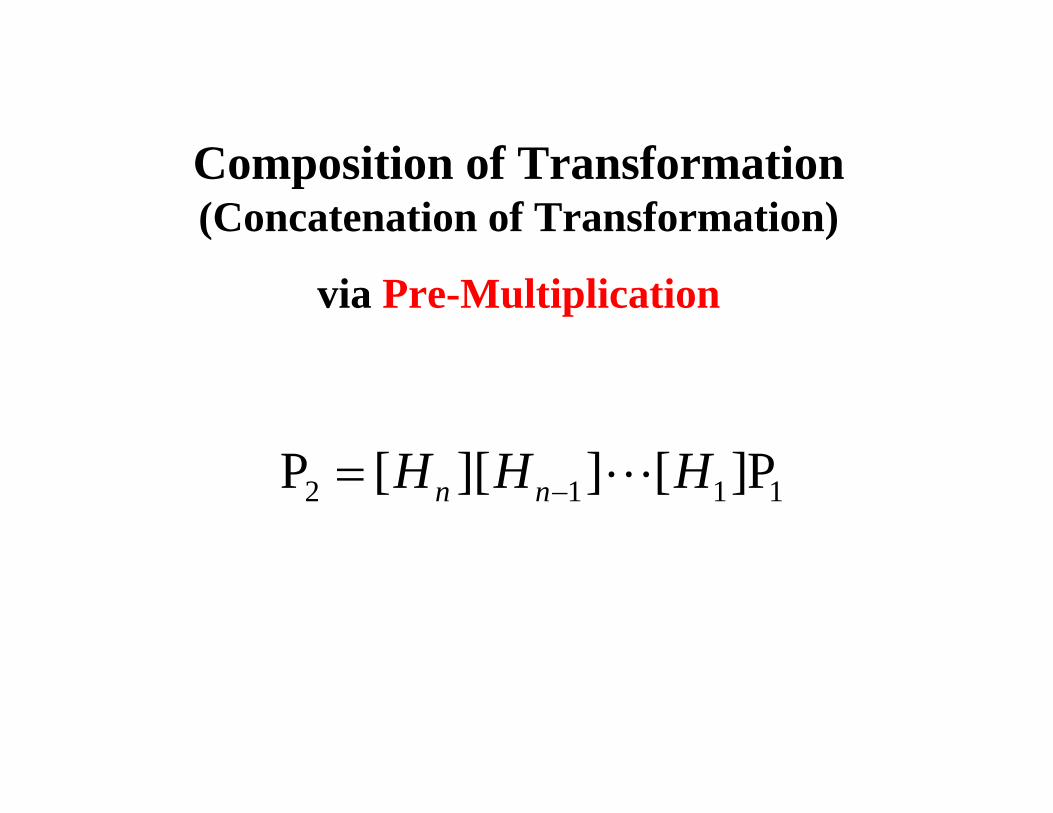
Composition of Transformation (Concatenation of Transformation)
via Pre-Multiplication
2 1 1 1P [ ][ ] [ ]Pn nH H H−=
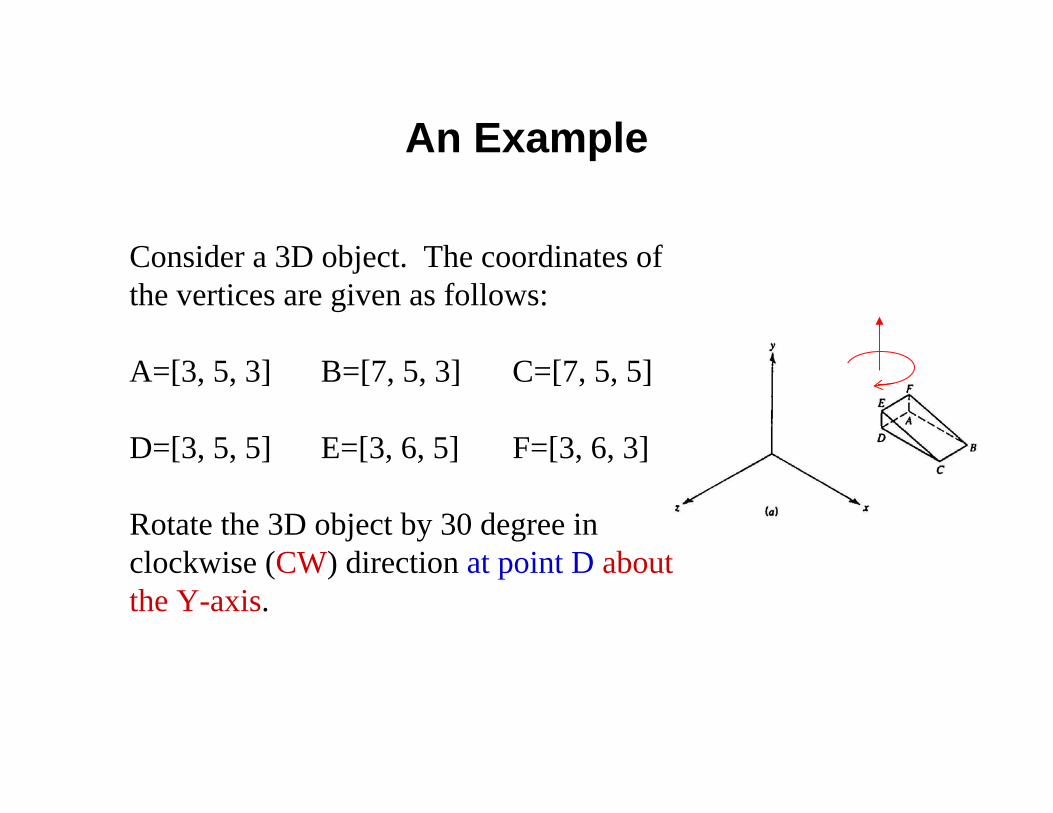
An Example
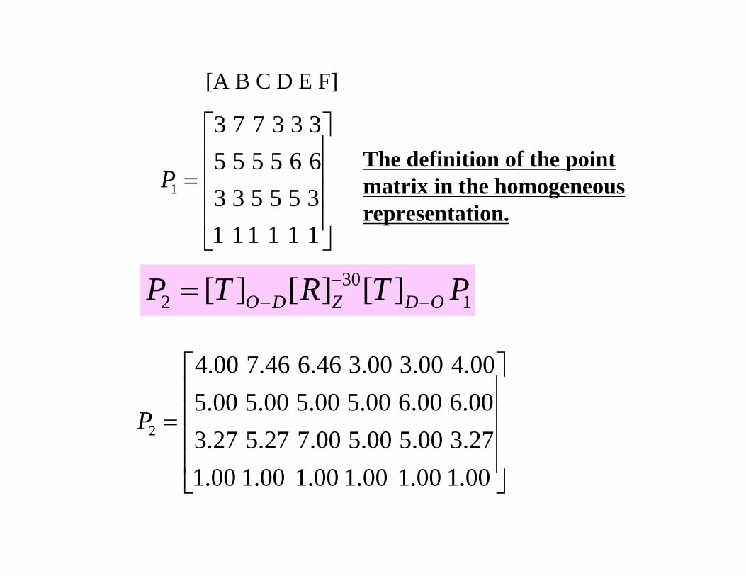
Consider a 3D object. The coordinates of the vertices are given as follows:
A=[3, 5, 3] B=[7, 5, 3] C=[7, 5, 5]
D=[3, 5, 5] E=[3, 6, 5] F=[3, 6, 3]
Rotate the 3D object by 30 degree in clockwise (CW) direction at point D about the Y-axis.
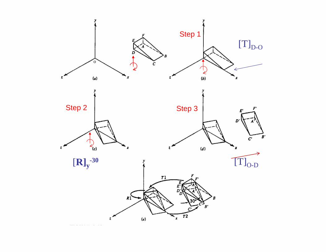
[T]D-O
[R]y-30 [T]O-D
Step 1
Step 2 Step 3
o
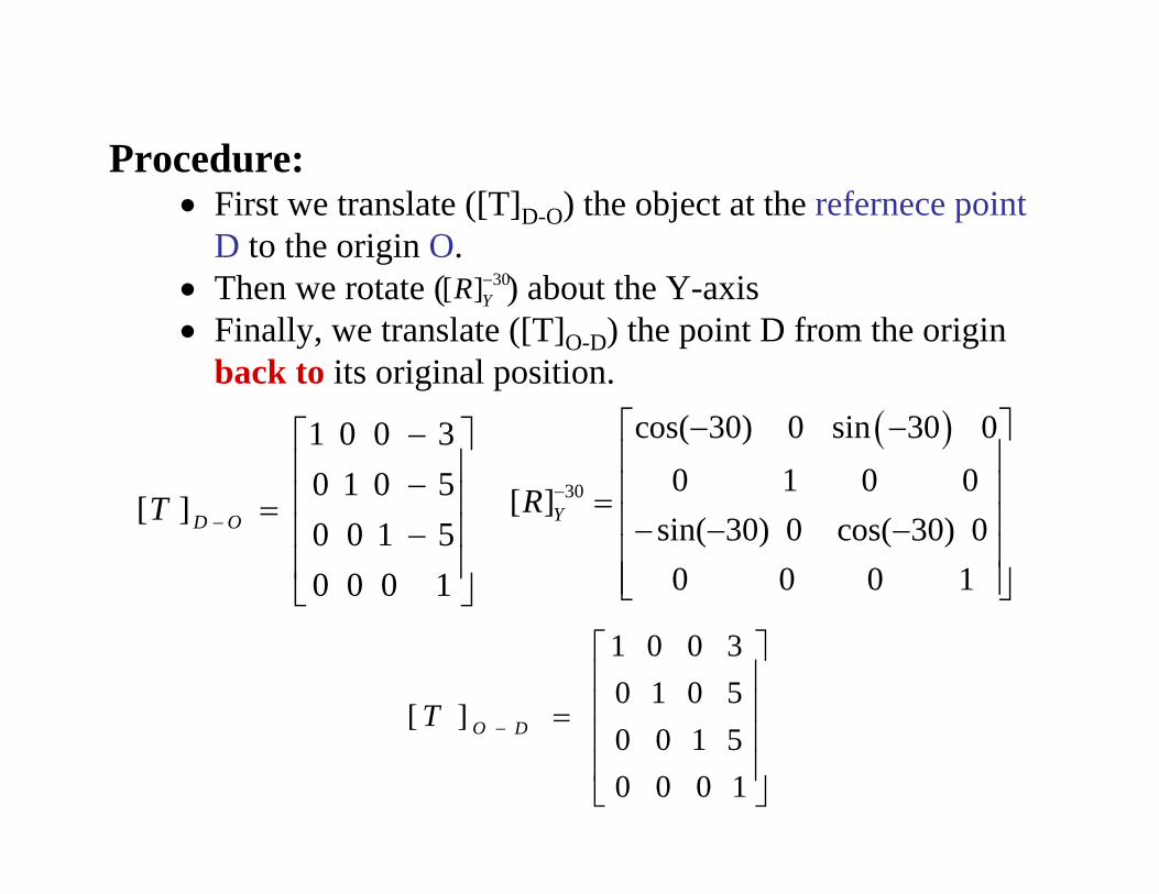
Procedure:• First we translate ([T]D-O) the object at the refernece point
D to the origin O.• Then we rotate ( ) about the Y-axis• Finally, we translate ([T]O-D) the point D from the origin
back to its original position.
1 0 0 30 1 0 5
[ ]0 0 1 50 0 0 1
D OT −
−⎡ ⎤⎢ ⎥−⎢ ⎥=⎢ ⎥−⎢ ⎥⎣ ⎦
( )30
cos( 30) 0 sin 30 00 1 0 0[ ]
sin( 30) 0 cos( 30) 00 0 0 1
YR −
− −⎡ ⎤⎢ ⎥⎢ ⎥=⎢ ⎥− − −⎢ ⎥⎢ ⎥⎣ ⎦
1 0 0 30 1 0 5
[ ]0 0 1 50 0 0 1
O DT −
⎡ ⎤⎢ ⎥⎢ ⎥=⎢ ⎥⎢ ⎥⎣ ⎦
30[ ]YR −
1
3 7 7 3 3 35 5 5 5 6 63 3 5 5 5 31 1 1 1 1 1
P
⎡ ⎤⎢ ⎥⎢ ⎥=⎢ ⎥⎢ ⎥⎣ ⎦
2
4.00 7.46 6.46 3.00 3.00 4.005.00 5.00 5.00 5.00 6.00 6.003.27 5.27 7.00 5.00 5.00 3.271.00 1.00 1.00 1.00 1.00 1.00
P
⎡ ⎤⎢ ⎥⎢ ⎥=⎢ ⎥⎢ ⎥⎣ ⎦
The definition of the point matrix in the homogeneous representation.
302 1[ ] [ ] [ ]O D Z D OP T R T P−
− −=
[A B C D E F]
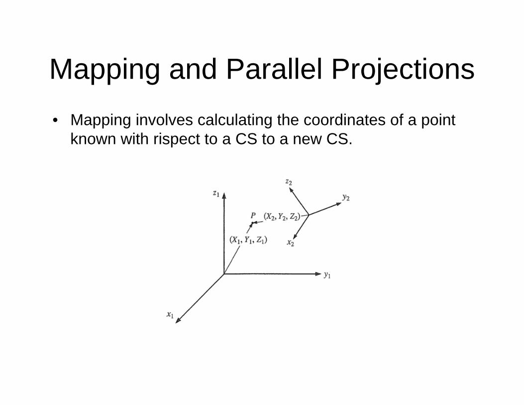
Mapping and Parallel Projections• Mapping involves calculating the coordinates of a point
known with rispect to a CS to a new CS.
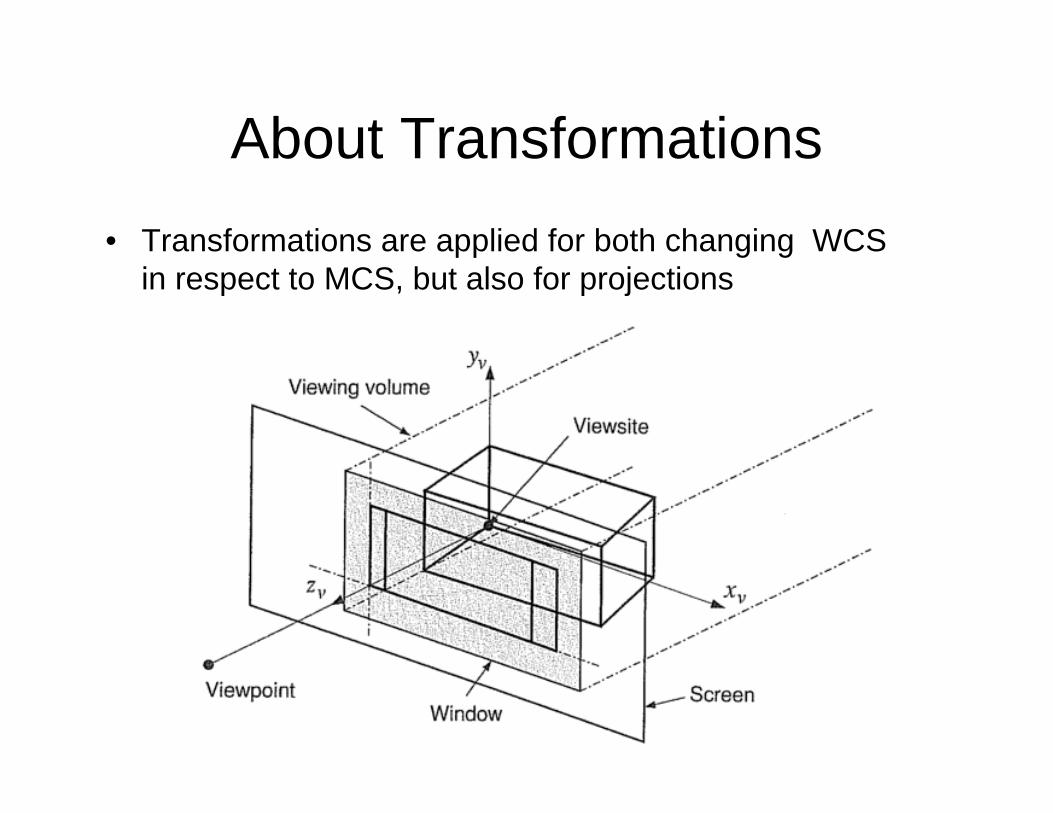
About Transformations• Transformations are applied for both changing WCS
in respect to MCS, but also for projections
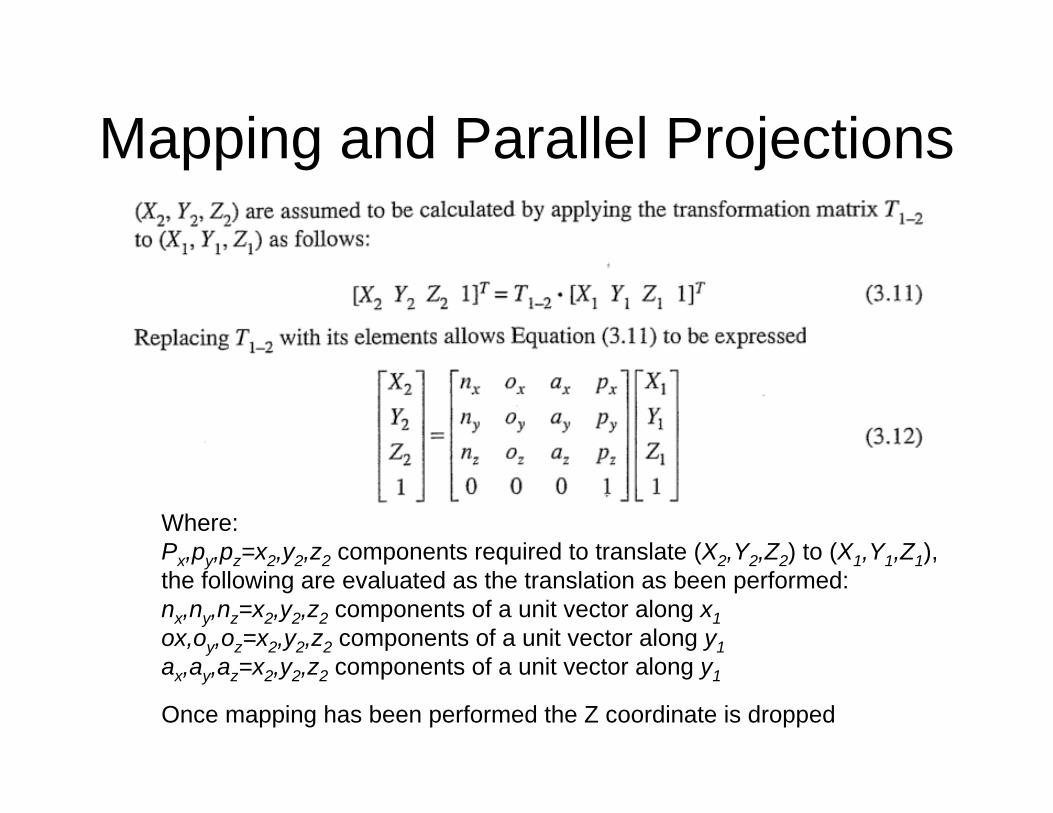
Mapping and Parallel Projections
Where:Px,py,pz=x2,y2,z2 components required to translate (X2,Y2,Z2) to (X1,Y1,Z1), the following are evaluated as the translation as been performed:nx,ny,nz=x2,y2,z2 components of a unit vector along x1ox,oy,oz=x2,y2,z2 components of a unit vector along y1ax,ay,az=x2,y2,z2 components of a unit vector along y1
Once mapping has been performed the Z coordinate is dropped
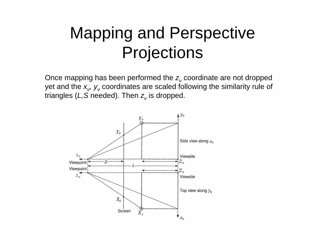
Mapping and Perspective Projections
Once mapping has been performed the zv coordinate are not dropped yet and the xv, yv coordinates are scaled following the similarity rule of triangles (L,S needed). Then zv is dropped.
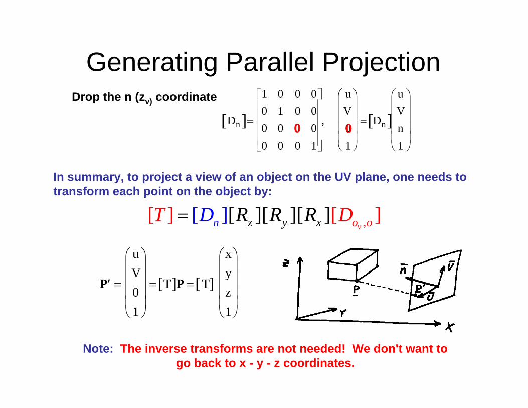
Generating Parallel Projection
Dn[ ]=
1 0 0 00 1 0 00 0 0 00 0 0 1
⎡
⎣
⎢ ⎢ ⎢ ⎢
⎤
⎦
⎥ ⎥ ⎥ ⎥
,
uV01
⎛
⎝
⎜ ⎜ ⎜ ⎜
⎞
⎠
⎟ ⎟ ⎟ ⎟
= Dn[ ]
uVn1
⎛
⎝
⎜ ⎜ ⎜ ⎜
⎞
⎠
⎟ ⎟ ⎟ ⎟
′ P =
uV01
⎛
⎝
⎜ ⎜ ⎜ ⎜
⎞
⎠
⎟ ⎟ ⎟ ⎟
= T[ ]P = T[ ]
xyz1
⎛
⎝
⎜ ⎜ ⎜ ⎜
⎞
⎠
⎟ ⎟ ⎟ ⎟
Drop the n (zv) coordinate
In summary, to project a view of an object on the UV plane, one needs to transform each point on the object by:
Note: The inverse transforms are not needed! We don't want to go back to x - y - z coordinates.
,[ ][[ ] [] ] ]][ [vz y o oxn R R DRDT =
0 0
FrontTop
Right
X
Y
Z
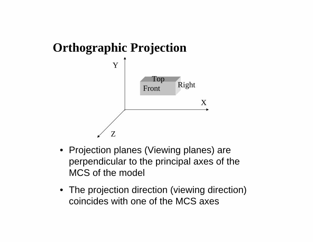
Orthographic Projection
• Projection planes (Viewing planes) are perpendicular to the principal axes of the MCS of the model
• The projection direction (viewing direction) coincides with one of the MCS axes
FrontTop
Right
X
Y
Z
Front
Yv,Y
Xv, X
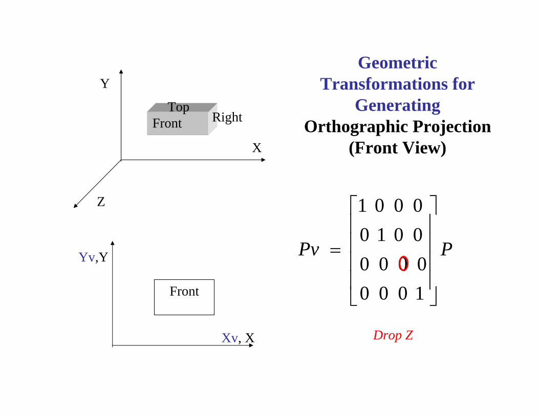
PPv
⎥⎥⎥⎥
⎦
⎤
⎢⎢⎢⎢
⎣
⎡
=
1000000000100001
Geometric Transformations for
Generating Orthographic Projection
(Front View)
Drop Z
FrontTop
Right
X
Y
Z
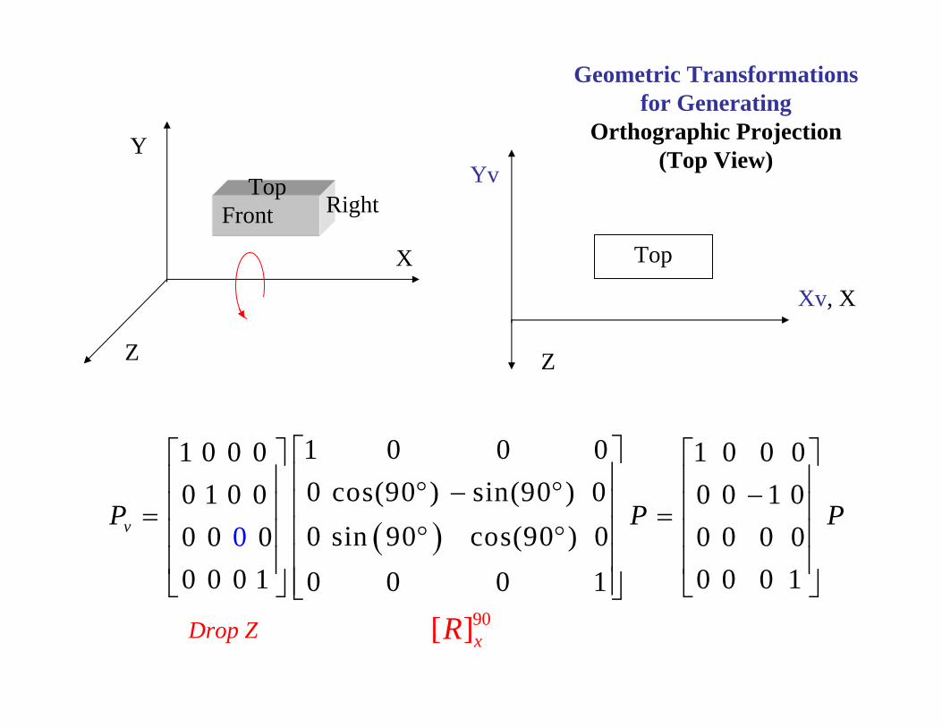
Top
Xv, X
Yv
Z
( )
1 0 0 01 0 0 0 1 0 0 00 cos(90 ) sin(90 ) 00 1 0 0 0 0 1 00 sin 90 cos(90 ) 00 0 0 0 0 0 0
0 0 0 1 0 0 0 10 0 0 10vP P P
⎡ ⎤⎡ ⎤ ⎡ ⎤⎢ ⎥⎢ ⎥ ⎢ ⎥° − ° −⎢ ⎥⎢ ⎥ ⎢ ⎥= =⎢ ⎥⎢ ⎥ ⎢ ⎥° °⎢ ⎥⎢ ⎥ ⎢ ⎥⎢ ⎥⎣ ⎦ ⎣ ⎦⎣ ⎦
Geometric Transformations for Generating
Orthographic Projection (Top View)
90[ ]xRDrop Z
FrontTop
Right
X
Y
Z
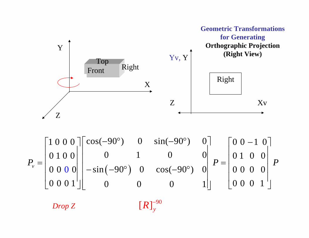
Right
Xv
Yv, Y
Z
( )
cos( 90 ) 0 sin( 90 ) 01 0 0 0 0 0 1 00 1 0 00 1 0 0 0 1 0 0
sin 90 0 cos( 90 ) 00 0 0 0 0 0 00 0 0 1 0 0 0 10 0 0 1
0vP P P
− ° − °⎡ ⎤ −⎡ ⎤ ⎡ ⎤⎢ ⎥⎢ ⎥ ⎢ ⎥⎢ ⎥⎢ ⎥ ⎢ ⎥= =⎢ ⎥⎢ ⎥ ⎢ ⎥− − ° − °⎢ ⎥⎢ ⎥ ⎢ ⎥⎢ ⎥⎣ ⎦ ⎣ ⎦⎣ ⎦
Geometric Transformations for Generating
Orthographic Projection (Right View)
90[ ]yR −Drop Z
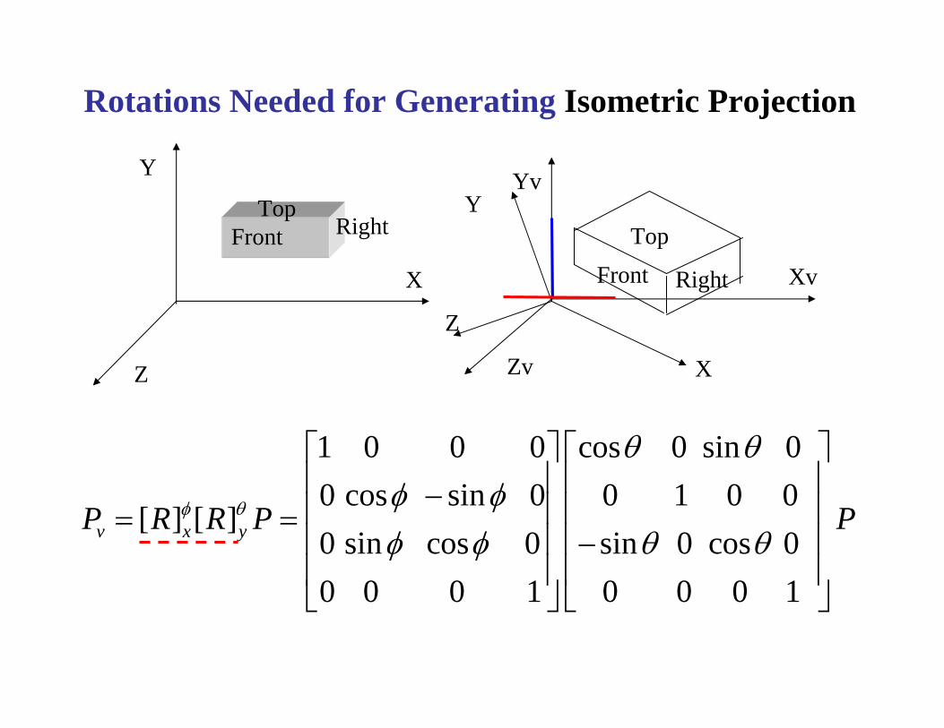
Rotations Needed for Generating Isometric Projection
1 0 0 0 cos 0 sin 00 cos sin 0 0 1 0 0
[ ] [ ]0 sin cos 0 sin 0 cos 00 0 0 1 0 0 0 1
v x yP R R P Pφ θ
θ θφ φφ φ θ θ
⎡ ⎤ ⎡ ⎤⎢ ⎥ ⎢ ⎥−⎢ ⎥ ⎢ ⎥= =⎢ ⎥ ⎢ ⎥−⎢ ⎥ ⎢ ⎥⎣ ⎦ ⎣ ⎦
Top
Right
Yv
Zv
Front
X
Z
Y
Xv
FrontTop
Right
X
Y
Z
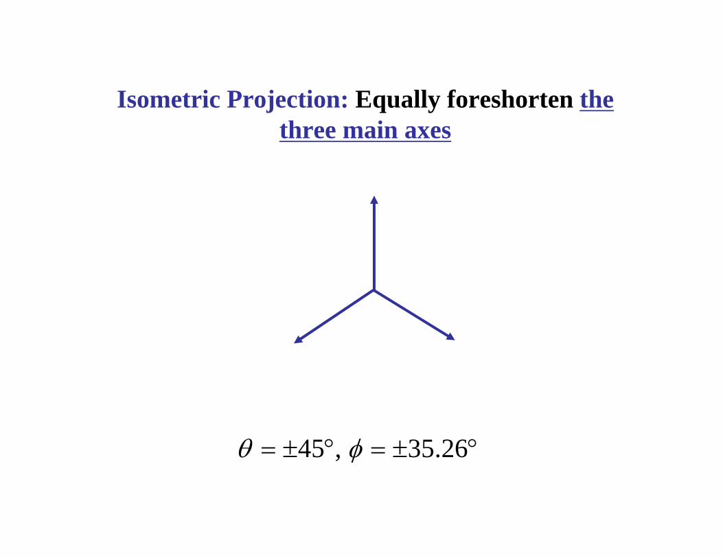
Isometric Projection: Equally foreshorten the three main axes
°±=°±= 26.35,45 φθ
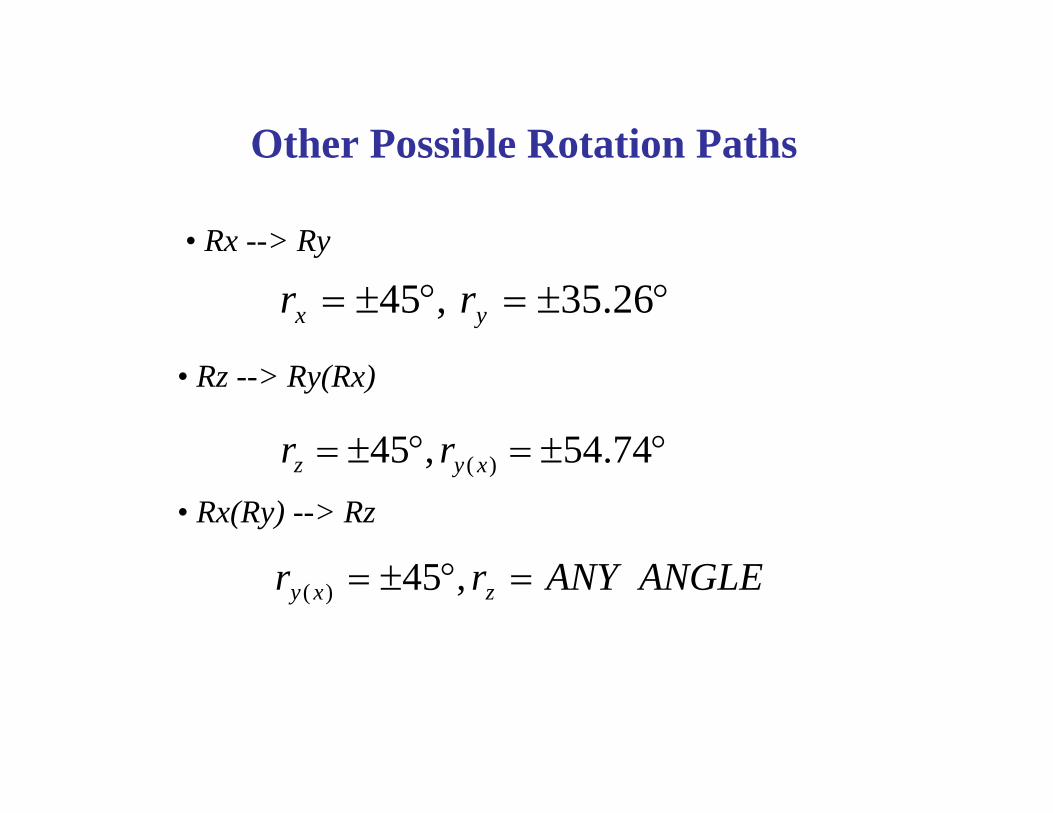
°±=°±= 26.35,45 yx rr• Rx --> Ry
• Rz --> Ry(Rx)
°±=°±= 74.54,45 )( xyz rr• Rx(Ry) --> Rz
ANGLEANYrr zxy =°±= ,45)(
Other Possible Rotation Paths