Embed Size (px)
Citation preview
Computers and Electrical Engineering 36 (2010) 503–517
Contents lists available at ScienceDirect
Computers and Electrical Engineering
journal homepage: www.elsevier .com/ locate/compeleceng
Controlling energy without compromising system performance inmobile grid environments
Li Chunlin *, Li LayuanDepartment of Computer Science, Wuhan University of Technology, Wuhan 430063, PR China
a r t i c l e i n f o
Article history:Received 10 November 2008Received in revised form 2 September 2009Accepted 9 December 2009Available online 6 January 2010
Keywords:GridSystem performanceMobile device
0045-7906/$ - see front matter � 2009 Elsevier Ltddoi:10.1016/j.compeleceng.2009.12.004
* Corresponding author.E-mail addresses: [email protected], jwtu@pu
a b s t r a c t
The challenges confronting in mobile grid systems are: limited CPU power, limitedmemory, small screen, short battery life, and intermittent disconnection. Considering allthese limitations, this paper is targeted to control energy consumption without compro-mising system’s performance in mobile grid. In this paper, we focus on using the mobiledevices on the mobile grid environment. Mobile devices can serve two important functionsin mobile grid environment either as service consumer or as valuable service providers. Theproposed approach is not only to reduce energy consumption, but also to improve systemperformance in mobile grid environment. Utility functions are used to express grid users’requirements, resource providers’ benefit function and system’s objectives. Dynamicprogramming is used to optimize the total utility function of mobile grid. A distributedcontrolling energy algorithm in mobile grid environment is proposed which decomposesmobile grid system optimization problem into sub-problems. In order to verify theefficiency of the proposed algorithm, in the experiment, the performance evaluation ofcontrolling energy algorithm is conducted.
� 2009 Elsevier Ltd. All rights reserved.
1. Introduction
Grid computing is based on the coordinated sharing of distributed and heterogeneous resources to solve large-scale prob-lems in dynamic virtual organizations. With the advent of high bandwidth third-generation mobile networks and other wire-less networks, grid computing has migrated from traditional parallel and distributed computing to pervasive and utilitycomputing based on the wireless networks and mobile devices, which results in the emergence of a new computing para-digm named mobile grid. The availability of wirelessly connected mobile devices has grown considerably in recent years.Having been constructed from a group of mobile devices, a mobile grid would allow the networked devices to accomplisha specific mission that maybe beyond an individual’s computing or communication capacity. Examples of applications of mo-bile Grids can be disaster management, wildfire fighting, and e-healthcare emergency, etc. The mobility of small, wirelessdevices creates tremendous opportunities to utilize the grid, and to enhance the services available on the grid. These mobiledevices differ from typical grid servers and clients in terms of communication and computation abilities, limited power con-straints, small screen, and the transitive nature of their connection to network infrastructures. In literature there are twoapproaches to integrate grid computing with mobile devices [1]. One approach is to allow these devices to access fixed gridresources that offer reliability, performance and quality of service. In this approach mobile devices cannot offer services togrid users but only can consume services. In second approach, mobile devices can consume services as well as can offer ser-vices to grid users. This approach also enables mobile devices to host grid management services instead of relying on fixed
. All rights reserved.
blic.wh.hb.cn (L. Chunlin).
504 L. Chunlin, L. Layuan / Computers and Electrical Engineering 36 (2010) 503–517
infrastructure. The capabilities of mobile devices are limited by their modest sizes and the finite lifetimes of the batteriesthat power them. As a result, minimizing the energy usage in mobile devices continues to pose significant challenges in mo-bile grid. In mobile grid, mobile devices are usually battery-driven. A limited energy budget restricts the computation andcommunication capacity of mobile device.
There are a number of challenging issues in using a mobile device as service consumer or a service provider in Grid sys-tems. The challenges confronting in mobile grid systems are: limited CPU power, limited memory, small screen, short batterylife, and intermittent disconnection. Considering all these limitations, this paper is targeted to control energy consumptionwithout compromising system’s performance in mobile grid. In this paper, we focus on using the mobile devices on the mo-bile grid environment. Mobile devices can serve two important functions in mobile grid environment either as service con-sumer or as valuable service providers. The proposed approach is not only to reduce energy consumption, but also toimprove system performance in mobile grid environment. Utility functions are used to express grid users’ requirements, re-source providers’ benefit function and system’s objectives. Dynamic programming is used to optimize the total utility func-tion of mobile grid. A distributed controlling energy algorithm in mobile grid environment is proposed which decomposesmobile grid system optimization problem into sub-problems. In order to verify the efficiency of the proposed algorithm, inthe experiment, the performance evaluation of controlling energy algorithm is conducted.
The rest of the paper is structured as following. Section 2 discusses the backgrounds and motivations. Section 3 presentscontrolling energy consumption without compromising system performance in mobile grid. Section 4 presents controllingenergy consumption algorithm in mobile grid. In section 5 the experiments are conducted and discussed. Section 6 givesthe conclusions to the paper.
2. Backgrounds and motivations
Currently, energy efficiency and optimization have been widely studied in communication system and high performancecomputing. Specially, economics method is used in wireless networks to deal with energy consumption such as [2–4,23,24].In [2], Zhou et al. have introduced a new routing algorithm, Utility-based Routing (UBR) algorithm, for ad-hoc wireless net-works. UBR adopts the microeconomic concepts of utility and pricing, and can balance energy consumption among all thenodes. This approach takes into account both energy efficiency and QoS constraint at the same time. In [3], Huang et al. haveaddressed the resource allocation problem in MANETs by using pricing to regulate individual nodes’ behaviors. Two pricingstrategies have been proposed, which take the factors of multiple transmission rates and energy consumptions into account.Pricing is a prospective direction to regulate behaviors of individual nodes while providing incentives for cooperation. Chenet al. [4] present a game-theoretic study on the power and rate control problem in IEEE 802.11 WLANs where network par-ticipants choose appropriate transmission power and data rate to achieve maximum throughput with minimum energy con-sumption. In such game-theoretic study, the central issues are the existence, uniqueness of the Nash equilibrium (NE), theconvergence to the NE and the system performance at the NE. In [5], Alsalih et al. propose a cooperative computing approachthat tackles the problem of energy limitation over MANETs. This paper formulates a novel energy-aware allocation problemand proposing a heuristic-based greedy algorithm to solve it approximately. The allocation algorithm assigns a set of com-putational tasks into a set of heterogeneous processors in such a way that minimizes the total consumed energy. In [6], Chenet al. discuss the problem of balancing energy consumption of the WSN with grid topology and propose a randomized datagathering scheme. In our scheme, direct transmission is tradeoff by hop-by-hop transmission so as to protect the sensornodes with higher load burden from early exhaustion. The network lifetime is thus prolonged. Shang et al. [7] present anew economics-based power-aware protocol, called the distributed economic sub-contracting protocol that dynamically dis-tributes task computation among mobile devices in an ad-hoc wireless network. The experimental results indicate that mar-kets based on the protocol and decision-making algorithms fairly and effectively allocate energy resources among differenttasks in both cooperative and competitive scenarios.
Park et al. [8] propose to exploit a grid infrastructure to extend the battery life of mobile devices based on the contexts ofmobile applications, devices, and grid systems. They present a framework, called SGA (selective grid access), to optimallyutilize the limited resources of mobile devices and grids. SGA aims to reconfigure the placement of mobile applicationson either the mobile device or grid nodes and to adjust QoS level according to the current context of the residual energyand the resource availability of the grids. Seshasayee et al. [9] discuss the problem of cooperative energy management indistributed mobile systems. It presents decentralized management techniques when running a distributed application ina MANET environment. Zong and Qin [10] design energy efficient scheduling algorithms for parallel applications runningon clusters, they propose a scheduling strategy called energy efficient task duplication schedule, which can significantly con-serve power by judiciously shrinking communication energy cost when allocating parallel tasks to heterogeneous computingnodes. Huang et al. [11] present techniques for exploiting intermittently available resources in grid infrastructures to sup-port QoS-based multimedia applications on mobile devices. They integrate power aware admission control, grid resourcediscovery, dynamic load-balancing and energy adaptation techniques to enable power deficient devices such as to run dis-tributed multimedia applications. Hoon Kim et al. [12] provide power-aware scheduling algorithms for bag of tasks applica-tions with deadline constraints on DVS enabled cluster systems in order to minimize power consumption as well as to meetthe deadlines specified by application users. Khan et al. [14] study the problem of allocation of tasks onto a computationalgrid, with the aim to simultaneously minimize the energy consumption and the makespan subject to the constraints of
L. Chunlin, L. Layuan / Computers and Electrical Engineering 36 (2010) 503–517 505
deadlines and tasks’ architectural requirements. They propose a solution from cooperative game theory based on the conceptof Nash bargaining solution (NBS). In [15], Katsaros et al. formulated the problem of job scheduling in a mobile grid environ-ment considering the problems incurred by intermittent connectivity. They proposed the installments scheduling policy spe-cifically tailored for the constrained mobile and wireless networking environment. The works [16–20] mainly deal withresource allocation, QoS optimization in the computational grid and do not consider energy consumption for mobile grid.The methods and contributions of this paper are different from above works. This paper is targeted to manage energy con-sumption without compromising system’s performance in mobile grid.
3. Controlling energy without compromising system performance in mobile grid
3.1. Problem formulation
Formulating the grid resource scheduling problem in economic terms is attractive for several reasons. First, resourceusage is not free. Grid resource cost must be considered when the grid is to become pervasive. Second, the dynamics of mo-bile grid are difficult to model. Application schedulers can make resource acquisition decisions at machine speeds in re-sponse to the perceived effects of contention. As resource load fluctuates, applications can adjust their resource usage,forming a feedback control loop with a potentially nonlinear response. The paper formulates controlling energy algorithmoptimization in mobile grid by adopting computational economy framework. The proposed model consists of two typesof roles: the grid resource agents that represent the economic interests of the underlying resources providers of the mobilegrid, the grid user agents that represent the interests of grid user application using the grid to achieve goals. Interactionsbetween the two agent types are mediated by means of market mechanisms. Market mechanism in economics is basedon distributed self-determination, the variation of price reflects the supply and demand of resources, and market theoryin economics provides precise depiction for efficiency of resource scheduling. Utility concept from microeconomics andgame theory can be used in mobile grid. Utility is a measure of customer’s degree of satisfaction and can be modeled as afunction of quality of service he has received and as well as money he has paid.
In mobile grid, energy resources distribution and computation workloads are not balanced within mobile devices. Somemobile devices have spare energy; some mobile devices are energy exhausted. Devices that expend all their energy can onlybe recharged when they leave the network. Therefore, it is important for the mobile grid system to manage energy consump-tion without compromising system’s performance. Firstly, let consider the notations used in the following sections. el
i is theenergy obtained by grid application i from energy resource l. Cel is the capacity of energy resource l.Cnk is the capacity ofnetwork resource k. Ccj is the capacity of computing power j. tn
i is the time taken by the grid application i to completenth job. Pcj
i is the payments of the grid application i to the computing power j. Pnki is the payments of the grid application
i to the network resource k. Peli is the payments of the grid application i to energy resource l. Bi is the expense budget of grid
application i. erl is the energy consumption rate of energy resource l. eni is energy dissipation caused by grid application i’s nth
job. cqni is the computation task of ith grid application’ s nth job. bqn
i is the transmission task of ith grid application’ s nth job.eqn
i is the energy storage task of ith grid application’ s nth job. npk the price of network resource k. cpj is the price of com-puting resource j. epl is the price of energy resource l. Ti is the deadline given by the grid application i to complete its all jobs.yk
i is the network allocation obtained by grid application i from the network resource k. xji is the computing power obtained
by grid application i from computing power j.We assume that the mobile grid has heterogeneous nodes with different system performance rates and network condi-
tions. This means that the energy consumption of the mobile device can vary with the response time of the application andthe network bandwidth. We denote el
i is the consumed energy fraction of the energy l (e.g. a battery) by grid application i.Total consumed energy of all grid applications
PIi¼1el
i does not exceed the total capacity Cel of energy l. Thus the followingresource consumption constraint needs to be satisfied:
XI
i¼1
eli 6 Cel ð3:1Þ
Energy consumption rate of each node in the system is measured by Joule per unit time. Let eni be an energy dissipation
caused by grid application i’s nth job, tni is the execution time of job n of grid application i on the grid node. er is the energy
consumption rate of energy resource l. If the energy consumption is proportional to execution time of jobn, as is the casewith battery energy. We define the energy consumption of each application Ai as the sum of the energy consumed by N gridjobs
PNn¼1en
i . The energy consumption of all grid jobs of each application Ai should be less than the available resources of eli
which is limited energy budget of grid user application i. For each grid application Ai, the consumed energy of all grid jobs ofAi should satisfy
XN
n¼1
eni 6 el
i ð3:2Þ
Now, we formulate the problem of controlling energy consumption in mobile grid as constraint optimization problem, theutility of the mobile grid Umobilegrid is defined as the sum of grid application utilities.
506 L. Chunlin, L. Layuan / Computers and Electrical Engineering 36 (2010) 503–517
Umobilegrid ¼XI
i¼1
Uiðeli; x
ji; y
ki Þ
where eli is the energy obtained by grid application i from the energy l. xj
i is CPU allocation obtained by grid applica-tion i from the computing resource provider j. yk
i is bandwidth allocation obtained by grid application i from the net-work resource provider k. The utility function for application Ai depends on allocated resources xj
i, yki and consumed
energy eli. The objective of controlling energy consumption in mobile grid is to maximize the utility of the mobile grid
Umobilegrid. By using nonlinear optimization theory, our controlling energy consumption in mobile grid can be formu-lated as follows.
Max Umobilegrid
s:t: Bi PXL
l¼1
Peli þXJ
j¼1
Pcji þXK
k¼1
Pnki ;
XI
i¼1
eli 6 Cel
Ti PXN
n¼1
tni ; Cnk P
XI
i¼1
yki ;
XN
n¼1
eni 6 el
i; Ccj PXI
i¼1
xji
ð3:3Þ
In the problem Eq. (3.3), the first type of constraints is related with different resource capacity. The QoS constraint impliesthat the aggregate network resource units
PIi¼1yk
i do not exceed the total capacity Cnk of network resource provider k, aggre-gate consumed energy of all grid application
PIi¼1el
i does not exceed the total Cel of energy l, aggregate computing powerPIi¼1xj
i does not exceed the total resource Ccj of the computing resource provider j. The second type of constraints is relatedwith grid application expense budget. Grid application needs to complete a sequence of jobs in a specified amount of time, Ti,while the payment overhead accrued cannot exceed Bi, which is the expense budget of grid application i. Pel
i; Pcji; Pnk
i are thepayments of the grid application i to the energy storage providerl, computing resource provider j and network resource pro-vider k. The total payments of the grid application i
PLl¼1Pel
i þPJ
j¼1Pcji þPK
k¼1Pnki dose not exceed Bi. The total energy con-
sumed by all jobs of grid application iPN
n¼1eni cannot exceed the energy budget el
i which is the available energy obtainedby grid application i from the energy storage l.
We apply the Lagrangian method to solve such a problem Eq. (3.3). The Lagrangian approach can be used to solve con-strained optimization problems. Let us consider the Lagrangian form of controlling energy consumption problem in mobilegrid:
L ¼XI
i¼1
Uiðeli; x
ji; y
ki Þ � ki
XI
i¼1
eli � Cel
!� bi
XI
i¼1
xji � Ccj
!�ui
XI
i¼1
yki � Cnk
!
� ci
XL
l¼1
Peli þXJ
j¼1
Pcji þXK
k¼1
Pnki � Bi
!� li
XN
n¼1
eni � el
i
!� ai
XN
n¼1
tni � Ti
!ð3:4Þ
where ki, bi and ui are the Lagrange multipliers of grid application with their interpretation of energy price, computing re-source capacity price, and network resource capacity price, respectively. Since the Lagrangian is separable, this maximizationof Lagrangian over (xj
i, yki , el
i) can be conducted in parallel at each application Ai. In problem Eq. (3.3), though the allocatedresources xj
i, yki and consumed energy el
i are coupled in their constraints, respectively, but they are separable. Given thatthe grid knows the utility functions U of all the grid applications, this optimization problem can be mathematically tractable.However, in practice, it is not likely to know each application’s utility, and it is also infeasible for mobile grid environment tocompute and allocate resources in a centralized fashion. In order to derive a distributed algorithm to solve problem Eq. (3.3),we decompose the problem into the sub-problems.
The mobile grid utility denoted as the sum of grid application utility can be defined as follows Eq. (3.5):
Umobilegrid ¼XI
i¼1
Uiðeli; x
ji; y
ki Þ
¼ Bi �XL
l¼1
Peli �XJ
j¼1
Pcji �XK
k¼1
Pnki
!þ Ti �
XN
n¼1
tni
!þXI
i¼1
ðPeli log el
i þ Pcji log xj
i þ Pnki log yk
i Þ þ eli �XN
n¼1
eni
!
ð3:5Þ
Mobile grid utility function is maximally optimized with specific constraints. In Eq. (3.5), Peli log el
i þ Pcji log xj
i þ Pnki log yk
i
present the revenue of energy storage resource, computing power and network resource provider. We could have chosen anyother form for the utility that increases with xj
i; yki ; e
li. But we chose the log function because the benefit increases quickly
from zero as the total allocated resource increases from zero and then increases slowly. Moreover, log function is analyticallyconvenient, increasing, strictly concave and continuously differentiable. The benefits of grid resource provider are affected bypayments of grid applications and allocated resources. It means that the revenue increases with increasing allocatedresources and increasing payment.
L. Chunlin, L. Layuan / Computers and Electrical Engineering 36 (2010) 503–517 507
The Lagrangian form of the problem Eq. (3.3) can be reformulated as follows Eq. (3.6):
L ¼ Bi �XL
l¼1
Peli �XJ
j¼1
Pcji �XK
k¼1
Pnki
!þXI
i¼1
ðPeli log el
i þ Pcji log xj
i þ Pnki log yk
i Þ þ Ti �XN
n¼1
tni
!þ el
i �XN
n¼1
eni
!
� ki
XI
i¼1
eli � Cel
!� bi sumI
i¼1xji � Ccj
� ��ui
XI
i¼1
yki � Cnk
!� ci
XL
l¼1
Peli þXJ
j¼1
Pcji þXK
k¼1
Pnki � Bi
!
� li
XN
n¼1
eni � el
i
!� ai
XN
n¼1
tni � Ti
!ð3:6Þ
The system model presented by Eq. (3.3) is a nonlinear optimization problem with N decision variables. Since theLagrangian is separable, the maximization of the Lagrangian can be processed in parallel for grid user applications and gridresource providers respectively. From Eq. (3.6), the resource allocation {el
i, xji, yk
i } solves problem Eq. (3.3) if and only if thereexist a set of nonnegative shadow costs {ki,bi,ui}. Generally solving such a problem by typical algorithms such as steepestdecent method and gradient projection method is of high computational complexity, which is very time costing and imprac-tical for implementation. In order to reduce the computational complexity, we decompose the utility optimization problemEq. (3.3) into two sub-problems for grid user applications and grid resource providers so that the computational complexityis reduced. The shadow costs suggest a mechanism to distribute the resource optimization between the grid applications andthe grid system. The problem Eq. (3.3) maximizes the utility of grid applications on the energy price, computing powercapacity price, and network resource capacity price,
PIi¼1Uiðel
i; xji; y
ki Þ is the total utility of mobile grid system, bi
PIi¼1xj
i isthe computing power cost, ki
PIi¼1el
i is the energy cost, ui
PIi¼1yk
i is the network resource cost. By decomposing the Kuhn–Tucker conditions into separate roles of consumer and supplier at grid market, the centralized problem Eq. (3.3) can be trans-formed into a distributed problem. Grid application’s payment is collected by the resource providers. The payments of gridapplications paid to resource providers are the payments to resolve the optimality of resource allocation in the grid market.We decompose the problem into the following two sub-problems Eq. (3.7) which is grid users optimization problem and Eq.(3.8) which is grid resource providers optimization problem, seek a distributed solution where the grid resource providerdoes not need to know the utility functions of individual grid user application. Eqs. (3.7) and (3.8) derived from the distrib-uted approach are identical to the optimal conditions given by centralized controlling energy consumption problem Eq. (3.3).This means if two sub-problems converge to its optimal points, then a globally optimal point is achieved. Total user appli-cation benefit of the mobile grid is maximized when the equilibrium prices, obtained through the two sub-problems Eqs.(3.7) and (3.8), equal the Lagrangian multipliers ki, bi and ui, where ki, bi and ui are the optimal prices charged by resourceproviders including energy, computing power and network resource to grid applications. Two maximization sub-problemscorrespond to grid application optimization problem as denoted by Eqs. (3.7) and (3.8).
Max UGA ¼ Bi �XL
l¼1
Peli �XJ
j¼1
Pcji �XK
k¼1
Pnki
!þ Ti �
XN
n¼1
tni
!þ el
i �XN
n¼1
eni
!XN
n¼1
eni 6 el
i; Ti PXN
n¼1
tni ;Bi
PXL
l¼1
Peli þXJ
j¼1
Pcji þXK
k¼1
Pnki ð3:7Þ
Max UGR ¼XI
i¼1
ðPeli log el
i þ Pcji log xj
i þ Pnki log yk
i ÞXI
i¼1
eli 6 Cel;Ccj P
XI
i¼1
xji; Cnk P
XI
i¼1
yki ð3:8Þ
In Eq. (3.7), the grid application gives the unique optimal payment to resource provider under the energy budget, expense
budget and the deadline constraint to maximize the user’s satisfaction. Bi �PL
l¼1Peli �PJ
j¼1Pcji �PK
k¼1Pnki
� �represents the
money surplus of grid application i, which is obtained by expense budgets subtracting the payments to various resource pro-
viders. Ti �PN
n¼1tni
� �represents the saving times for grid application i, which is gotten by time limit subtracting actual
spending time. eli �P
neni
� �represents the energy surplus of grid application i which is obtained by the energy budgets sub-
tracting actual energy dissipation. So, the objective of Eq. (3.7) is to get more surpluses of money and more energy savings, atthe same time, complete task for grid user application as soon as possible. In Eq. (3.8), different resource providers compute
optimal resource allocation for maximizing the revenue of their own. Grid application i submits the payment Peli to the en-
ergy resource providerl, Pnki to network resource provider k and Pcj
i to computing power provider j. Peli log el
i presents the rev-
enue obtained by energy resource l from grid application i. Pcji log xj
i presents the revenue obtained by computing power j
from grid application i. Pnki log yk
i presents the revenue obtained by network resource k from grid application i. The objective
of resource providers is to maximize Peli log el
i þ Pcji log xj
i þ Pnki log yk
i under the constraints of their provided resourceamounts. Grid resource providers cannot sell the resources to grid applications more than total capacity. In Eq. (3.7), the gridapplication adaptively adjusts its payments to computing power, network resource and energy based on the current resourceconditions, while in Eq. (3.8), the grid resource provider adaptively allocates energy, CPU and bandwidth required by the gridapplication in the Eq. (3.7). The interaction between two sub-problems is controlled through the use of the price variable ki,
508 L. Chunlin, L. Layuan / Computers and Electrical Engineering 36 (2010) 503–517
bi and ui, which is the energy price, computing power price, and network resource price charged from grid applications bygrid energy resource, computing power and network resource. The interaction between two sub-problems also coordinatesthe grid application’s payment and the supply of grid resource providers.
3.2. Optimization solutions
Controlling energy consumption optimization problem involves variables from grid applications and resource providers.Lagrange relaxation and gradient optimization can be applied to decompose such an overall optimization problem into asequence of two sub-problems, each only involving variables from the grid application and resource providers respec-tively. In Eq. (3.7), grid application maximizes its satisfaction and gives the unique optimal payment to resource providerunder the energy budget, expense budget and the deadline constraint. We assume that grid application i submits Pel
i toenergy resource l, Pcj
i to computing power j and Pnki to network resource k. Then, Pei ¼ ½Pe1
i . . . Peli� represents all payments
of grid applications for energy resource l, Pci ¼ ½Pc1i . . . Pcj
i� represents all payments of grid applications for computingpower j, Pni ¼ ½Pn1
i . . . Pnki � represents all payments of grid applications for the network resource k. Let
mi ¼P
lPeli þP
jPcji þP
kPnki , mi is the total payment of the ith grid application. N grid applications compete for grid re-
sources with finite capacity. The resource is allocated using a market mechanism, where the partitions depend on the rel-ative payments sent by the grid applications. Let epl, cpj, npk denote the price of the resource unit of energy resource l, theprice of the resource unit of computing power j and network resource k, respectively. Let the pricing policy, ep = (e-p1,ep2, . . . ,epl), denote the set of resource unit prices of all the energy resources in the grid, cp = (cp1,cp2, . . . ,cpj), denotethe set of resource unit prices of all the computing powers, np = (np1,np2, . . . ,npk) is set of network resource unit prices.The ith grid application receives the resources proportional to its payment relative to the sum of the resource provider’srevenue. Let el
i, xji, yk
i be the fraction of resource units allocated to grid application i by energy l, computing power j andnetwork resource k.
xji ¼ Ccj
Pcji
cpj; el
i ¼ CelPel
i
epl; yk
i ¼ CnkPnk
i
npk
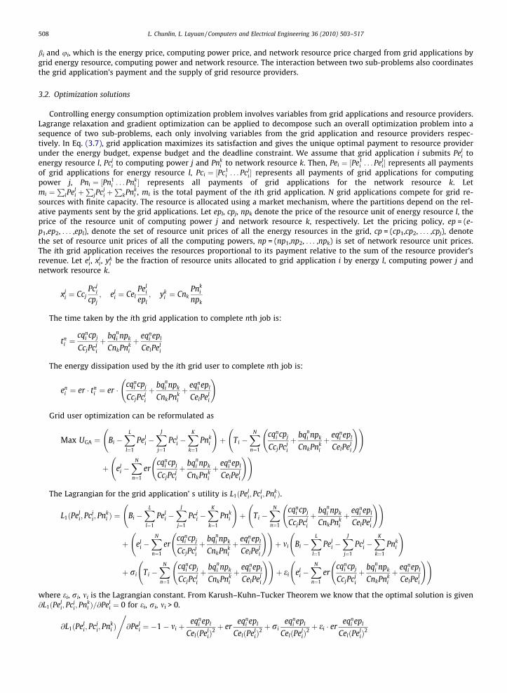
The time taken by the ith grid application to complete nth job is:
tni ¼
cqni cpj
CcjPcji
þ bqni npk
CnkPnki
þ eqni epl
CelPeli
The energy dissipation used by the ith grid user to complete nth job is:
eni ¼ er � tn
i ¼ er �cqn
i cpj
CcjPcji
þ bqni npk
CnkPnki
þ eqni epl
CelPeli
!
Grid user optimization can be reformulated as
Max UGA ¼ Bi �XL
l¼1
Peli �XJ
j¼1
Pcji �XK
k¼1
Pnki
!þ Ti �
XN
n¼1
cqni cpj
CcjPcji
þ bqni npk
CnkPnki
þ eqni epl
CelPeli
! !
þ eli �XN
n¼1
ercqn
i cpj
CcjPcji
þ bqni npk
CnkPnki
þ eqni epl
CelPeli
! !
The Lagrangian for the grid application’ s utility is L1ðPeli; Pcj
i; Pnki Þ.
L1ðPeli; Pcj
i; Pnki Þ ¼ Bi �
XL
l¼1
Peli �XJ
j¼1
Pcji �XK
k¼1
Pnki
!þ Ti �
XN
n¼1
cqni cpj
CcjPcji
þ bqni npk
CnkPnki
þ eqni epl
CelPeli
! !
þ eli �XN
n¼1
ercqn
i cpj
CcjPcji
þ bqni npk
CnkPnki
þ eqni epl
CelPeli
! !þ mi Bi �
XL
l¼1
Peli �XJ
j¼1
Pcji �XK
k¼1
Pnki
!
þ ri Ti �XN
n¼1
cqni cpj
CcjPcji
þ bqni npk
CnkPnki
þ eqni epl
CelPeli
! !þ ei el
i �XN
n¼1
ercqn
i cpj
CcjPcji
þ bqni npk
CnkPnki
þ eqni epl
CelPeli
! !
where ei, ri, mi is the Lagrangian constant. From Karush–Kuhn–Tucker Theorem we know that the optimal solution is given@L1ðPel
i; Pcji; Pnk
i Þ=@Peli ¼ 0 for ei, ri, mi > 0.
@L1ðPeli; Pcj
i; Pnki Þ @Pel
i ¼ �1� mi þeqn
i epl
CelðPeliÞ
2 þ ereqn
i epl
CelðPeliÞ
2 þ rieqn
i epl
CelðPeliÞ
2 þ ei � ereqn
i epl
CelðPeliÞ
2
,
L. Chunlin, L. Layuan / Computers and Electrical Engineering 36 (2010) 503–517 509
Let @L1ðPeli; Pcj
i; Pnki Þ.@Pel
i ¼ 0 to obtain
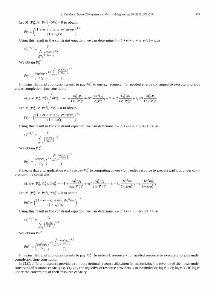
Peli ¼
ð1þ er þ ri þ ei � erÞeqni epl
ð1þ miÞCel
� �1=2
Using this result in the constraint equation, we can determine h = (1 + er + ri + ei � er)/1 + mi as
ðhÞ�1=2 ¼ TiPNm¼1
epmeqni
Cem
� �1=2
We obtain Peli
�
Peli
�¼ eqn
i epl
Cel
� �1=2PN
m¼1
eqni
epm
Cem
� �1=2
Ti
It means that grid application wants to pay Peli
�to energy resource l for needed energy consumed to execute grid jobs
under completion time constraint.
@L1ðPeli; Pcj
i; Pnki Þ @Pcj
i ¼ �1þcqn
i cpj
CcjðPcjiÞ
2 þ erni
cqni cpj
CcjðPcjiÞ
2 � mi þ ricqn
i cpj
CcjðPcjiÞ
2 þ ei � ercqn
i cpj
CcjðPcjiÞ
2
,
Let @L1ðPeli; Pcj
i; Pnki Þ=@Pcj
i ¼ 0 to obtain
Pcji ¼
ð1þ er þ ri þ ei � erÞcqni cpj
ð1þ miÞCcj
� �1=2
Using this result in the constraint equation, we can determine n = (1 + er + ri + ei.er)/1 + mi as
ðnÞ�1=2 ¼ TiPNm¼1
cpmcqni
Ccm
� �1=2
We obtain Pcji
�
Pcji
�¼
cqni cpj
Ccj
� �1=2PN
m¼1
cqni
cpm
Ccm
� �1=2
Ti
It means that grid application wants to pay Pcji
�to computing power j for needed resource to execute grid jobs under com-
pletion time constraint.
@L1ðPeli; Pcj
i; Pnki Þ=@Pnk
i ¼ �1þ bqni npk
CnkðPnki Þ
2 þ erni
bqni npk
CnkðPnki Þ
2 � mi þ ribqn
i npk
CnkðPnki Þ
2 þ eibqn
i npk
CnkðPnki Þ
2
Let @L1ðPeli; Pcj
i; Pnki Þ=@Pnk
i ¼ 0 to obtain
Pnki ¼
ð1þ er þ ri þ er:eiÞbqni npk
ð1þ miÞCnk
� �1=2
Using this result in the constraint equation, we can determine s = (1 + er + ri + er.ei)/1 + mi as
ðsÞ�1=2 ¼ TiPNm¼1
npmbqni
Cnm
� �1=2
We obtain Pnki
�
Pnki
�¼ bqn
i npk
Cnk
� �1=2PN
m¼1
bqni npm
Cnm
� �1=2
Ti
It means that grid application wants to pay Pnki
�to network resource k for needed resource to execute grid jobs under
completion time constraint.In (3.8), different resource providers compute optimal resource allocation for maximizing the revenue of their own under
constrains of resource capacity Cel, Ccj, Cnk, the objective of resource providers is to maximize Peli log el
i þ Pcji log xj
i þ Pnki log yk
i
under the constraints of their resource capacity.
510 L. Chunlin, L. Layuan / Computers and Electrical Engineering 36 (2010) 503–517
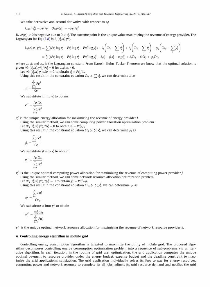
We take derivative and second derivative with respect to xi:
UGR0ðeliÞ ¼ Pel
i=eji UGR00ðel
iÞ ¼ �Peli=el2
i
UGR00ðeliÞ < 0 is negative due to 0 < el
i. The extreme point is the unique value maximizing the revenue of energy provider. TheLagrangian for Eq. (3.8) is L2ðel
i; xji; y
ki Þ.
L2ðeli; x
ji; y
ki Þ ¼
XðPel
i log eli þ Pcj
i log xji þ Pnk
i log yki Þ þ ki Cel �
Xi
eli
!þ bi Ccj �
Xi
xji
!þui Cnk �
Xi
yki
!
¼XðPel
i log eli þ Pcj
i log xji þ Pnk
i log yki � kiel
i � bixji �uiy
ki Þ þ kiCel þ biCcj þuiCnk
where ki, bi and ui, is the Lagrangian constant. From Karush–Kuhn–Tucker Theorem we know that the optimal solution isgiven @L2ðel
i; xji; y
ki Þ=@el
i ¼ 0 for ki,bi,ui > 0.Let @L2ðel
i; xji; y
jiÞ=@el
i ¼ 0 to obtain eli ¼ Pel
i=ki.Using this result in the constraint equation Cel P
Pel
i, we can determine ki as
ki ¼
Pnd¼1
Pedi
Cel
We substitute k into eli to obtain
eli� ¼ Pel
iCelPnd¼1
Pedi
el�
i is the unique energy allocation for maximizing the revenue of energy provider l.Using the similar method, we can solve computing power allocation optimization problem.Let @L2ðel
i; xji; y
ki Þ=@xj
i ¼ 0 to obtain xji ¼ Pcj
i=bi
Using this result in the constraint equation Ccj PP
xji, we can determine bi as
bi ¼
Pnd¼1
Pcdi
Ccj
We substitute b into xji to obtain
xji
�¼ Pcj
iCcjPnd¼1
Pcdi
xji
�is the unique optimal computing power allocation for maximizing the revenue of computing power provider j.Using the similar method, we can solve network resource allocation optimization problem.Let @L2ðel
i; xji; y
ki Þ=@yk
i ¼ 0 to obtain yki ¼ Pnk
i =ui
Using this result in the constraint equation Cnk PP
yki , we can determine ui as
ui ¼
Pnd¼1
Pndi
Cnk
We substitute u into yki to obtain
yki� ¼ Pnk
i CnkPnd¼1
Pndi
yk�
i is the unique optimal network resource allocation for maximizing the revenue of network resource provider k.
4. Controlling energy algorithm in mobile grid
Controlling energy consumption algorithm is targeted to maximize the utility of mobile grid. The proposed algo-rithm decomposes controlling energy consumption optimization problem into a sequence of sub-problems via an iter-ative algorithm. In each iteration, in the routine of grid user optimization, the grid application computes the uniqueoptimal payment to resource provider under the energy budget, expense budget and the deadline constraint to max-imize the grid application’s satisfaction. The grid application individually solves its fees to pay for energy resources,computing power and network resource to complete its all jobs, adjusts its grid resource demand and notifies the grid
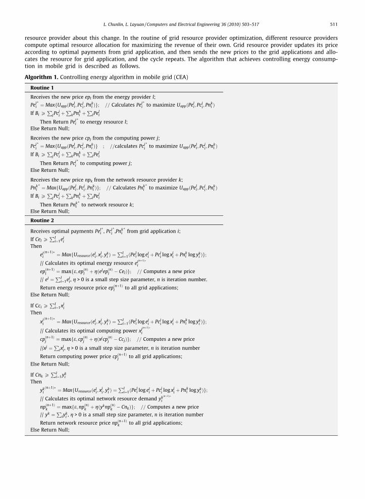
L. Chunlin, L. Layuan / Computers and Electrical Engineering 36 (2010) 503–517 511
resource provider about this change. In the routine of grid resource provider optimization, different resource providerscompute optimal resource allocation for maximizing the revenue of their own. Grid resource provider updates its priceaccording to optimal payments from grid application, and then sends the new prices to the grid applications and allo-cates the resource for grid application, and the cycle repeats. The algorithm that achieves controlling energy consump-tion in mobile grid is described as follows.
Algorithm 1. Controlling energy algorithm in mobile grid (CEA)
Routine 1
Receives the new price epl from the energy provider l;
Peli�¼ MaxfUappðPel
i; Pcji; Pnk
i Þg; == Calculates Peli�
to maximize UappðPeli; Pcj
i; Pnki Þ
If Bi PP
jPcji þP
kPnki þ
PlPel
i
Then Return Peli�
to energy resource l;Else Return Null;
Receives the new price cpj from the computing power j;
Pcji
�¼ MaxfUappðPel
i; Pcji;Pnk
i Þg ; ==calculates Pcji
�to maximize UappðPel
i; Pcji; Pnk
i ÞIf Bi P
PjPcj
i þP
kPnki þ
PlPel
i
Then Return Pcji
�to computing power j;
Else Return Null;
Receives the new price npk from the network resource provider k;
Pnki�¼ MaxfUappðPel
i; Pcji; Pnk
i Þg; == Calculates Pnki�
to maximize UappðPeli; Pcj
i; Pnki Þ
If Bi PP
jPcji þP
kPnki þ
PlPel
i
Then Return Pnki�
to network resource k;Else Return Null;
Routine 2
Receives optimal payments Peli�, Pcj
i
�,Pnk
i�
from grid application i;
If Cel PPI
i¼1eli
Then
eliðnþ1Þ� ¼ MaxfUresourceðel
i; xji; y
ki Þ ¼
PIi¼1ðPel
i log eli þ Pcj
i log xji þ Pnk
i log yki Þg;
// Calculates its optimal energy resource elðnþ1Þ�
i
epðnþ1Þl ¼ maxfe; epðnÞl þ gðelepðnÞl � CelÞg; == Computes a new price
// el ¼PI
i¼1eli, g > 0 is a small step size parameter, n is iteration number.
Return energy resource price epðnþ1Þl to all grid applications;
Else Return Null;
If Cci PPI
i¼1xji
Then
xji
ðnþ1Þ�¼ MaxfUresourceðel
i; xji; y
ki Þ ¼
PIi¼1ðPel
i log eli þ Pcj
i log xji þ Pnk
i log yki Þg;
// Calculates its optimal computing power xjðnþ1Þ�
i
cpðnþ1Þj ¼ maxfe; cpðnÞj þ gðxjcpðnÞj � CcjÞg; == Computes a new price
//xj ¼P
ixji , g > 0 is a small step size parameter, n is iteration number
Return computing power price cpðnþ1Þj to all grid applications;
Else Return Null;
If Cnk PPI
i¼1yki
Then
ykiðnþ1Þ� ¼ MaxfUresourceðel
i; xji; y
ki Þ ¼
PIi¼1ðPel
i log eli þ Pcj
i log xji þ Pnk
i log yki Þg;
// Calculates its optimal network resource demand ykðnþ1Þ�
i
npðnþ1Þk ¼maxfe;npðnÞk þ gðyknpðnÞk � CnkÞg; == Computes a new price
// yk ¼P
iyki , g > 0 is a small step size parameter, n is iteration number
Return network resource price npðnþ1Þk to all grid applications;
Else Return Null;
512 L. Chunlin, L. Layuan / Computers and Electrical Engineering 36 (2010) 503–517
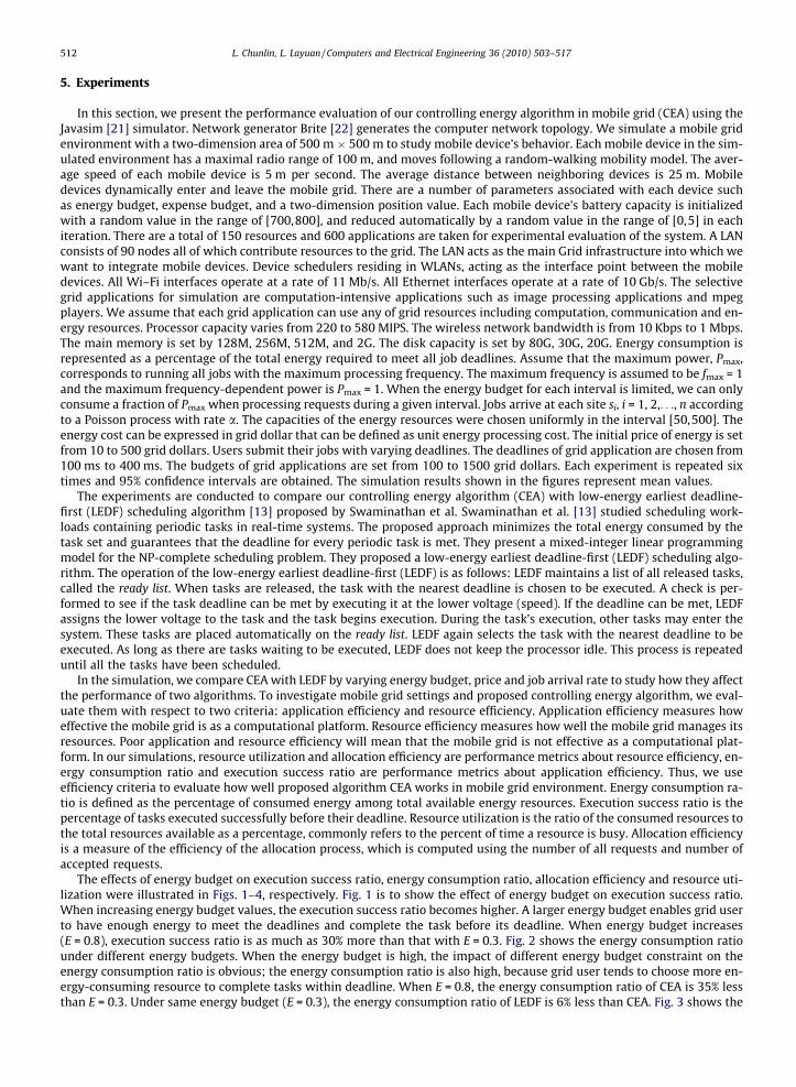
5. Experiments
In this section, we present the performance evaluation of our controlling energy algorithm in mobile grid (CEA) using theJavasim [21] simulator. Network generator Brite [22] generates the computer network topology. We simulate a mobile gridenvironment with a two-dimension area of 500 m � 500 m to study mobile device’s behavior. Each mobile device in the sim-ulated environment has a maximal radio range of 100 m, and moves following a random-walking mobility model. The aver-age speed of each mobile device is 5 m per second. The average distance between neighboring devices is 25 m. Mobiledevices dynamically enter and leave the mobile grid. There are a number of parameters associated with each device suchas energy budget, expense budget, and a two-dimension position value. Each mobile device’s battery capacity is initializedwith a random value in the range of [700,800], and reduced automatically by a random value in the range of [0,5] in eachiteration. There are a total of 150 resources and 600 applications are taken for experimental evaluation of the system. A LANconsists of 90 nodes all of which contribute resources to the grid. The LAN acts as the main Grid infrastructure into which wewant to integrate mobile devices. Device schedulers residing in WLANs, acting as the interface point between the mobiledevices. All Wi–Fi interfaces operate at a rate of 11 Mb/s. All Ethernet interfaces operate at a rate of 10 Gb/s. The selectivegrid applications for simulation are computation-intensive applications such as image processing applications and mpegplayers. We assume that each grid application can use any of grid resources including computation, communication and en-ergy resources. Processor capacity varies from 220 to 580 MIPS. The wireless network bandwidth is from 10 Kbps to 1 Mbps.The main memory is set by 128M, 256M, 512M, and 2G. The disk capacity is set by 80G, 30G, 20G. Energy consumption isrepresented as a percentage of the total energy required to meet all job deadlines. Assume that the maximum power, Pmax,corresponds to running all jobs with the maximum processing frequency. The maximum frequency is assumed to be fmax = 1and the maximum frequency-dependent power is Pmax = 1. When the energy budget for each interval is limited, we can onlyconsume a fraction of Pmax when processing requests during a given interval. Jobs arrive at each site si, i = 1, 2,. . ., n accordingto a Poisson process with rate a. The capacities of the energy resources were chosen uniformly in the interval [50,500]. Theenergy cost can be expressed in grid dollar that can be defined as unit energy processing cost. The initial price of energy is setfrom 10 to 500 grid dollars. Users submit their jobs with varying deadlines. The deadlines of grid application are chosen from100 ms to 400 ms. The budgets of grid applications are set from 100 to 1500 grid dollars. Each experiment is repeated sixtimes and 95% confidence intervals are obtained. The simulation results shown in the figures represent mean values.
The experiments are conducted to compare our controlling energy algorithm (CEA) with low-energy earliest deadline-first (LEDF) scheduling algorithm [13] proposed by Swaminathan et al. Swaminathan et al. [13] studied scheduling work-loads containing periodic tasks in real-time systems. The proposed approach minimizes the total energy consumed by thetask set and guarantees that the deadline for every periodic task is met. They present a mixed-integer linear programmingmodel for the NP-complete scheduling problem. They proposed a low-energy earliest deadline-first (LEDF) scheduling algo-rithm. The operation of the low-energy earliest deadline-first (LEDF) is as follows: LEDF maintains a list of all released tasks,called the ready list. When tasks are released, the task with the nearest deadline is chosen to be executed. A check is per-formed to see if the task deadline can be met by executing it at the lower voltage (speed). If the deadline can be met, LEDFassigns the lower voltage to the task and the task begins execution. During the task’s execution, other tasks may enter thesystem. These tasks are placed automatically on the ready list. LEDF again selects the task with the nearest deadline to beexecuted. As long as there are tasks waiting to be executed, LEDF does not keep the processor idle. This process is repeateduntil all the tasks have been scheduled.
In the simulation, we compare CEA with LEDF by varying energy budget, price and job arrival rate to study how they affectthe performance of two algorithms. To investigate mobile grid settings and proposed controlling energy algorithm, we eval-uate them with respect to two criteria: application efficiency and resource efficiency. Application efficiency measures howeffective the mobile grid is as a computational platform. Resource efficiency measures how well the mobile grid manages itsresources. Poor application and resource efficiency will mean that the mobile grid is not effective as a computational plat-form. In our simulations, resource utilization and allocation efficiency are performance metrics about resource efficiency, en-ergy consumption ratio and execution success ratio are performance metrics about application efficiency. Thus, we useefficiency criteria to evaluate how well proposed algorithm CEA works in mobile grid environment. Energy consumption ra-tio is defined as the percentage of consumed energy among total available energy resources. Execution success ratio is thepercentage of tasks executed successfully before their deadline. Resource utilization is the ratio of the consumed resources tothe total resources available as a percentage, commonly refers to the percent of time a resource is busy. Allocation efficiencyis a measure of the efficiency of the allocation process, which is computed using the number of all requests and number ofaccepted requests.
The effects of energy budget on execution success ratio, energy consumption ratio, allocation efficiency and resource uti-lization were illustrated in Figs. 1–4, respectively. Fig. 1 is to show the effect of energy budget on execution success ratio.When increasing energy budget values, the execution success ratio becomes higher. A larger energy budget enables grid userto have enough energy to meet the deadlines and complete the task before its deadline. When energy budget increases(E = 0.8), execution success ratio is as much as 30% more than that with E = 0.3. Fig. 2 shows the energy consumption ratiounder different energy budgets. When the energy budget is high, the impact of different energy budget constraint on theenergy consumption ratio is obvious; the energy consumption ratio is also high, because grid user tends to choose more en-ergy-consuming resource to complete tasks within deadline. When E = 0.8, the energy consumption ratio of CEA is 35% lessthan E = 0.3. Under same energy budget (E = 0.3), the energy consumption ratio of LEDF is 6% less than CEA. Fig. 3 shows the
0
20
40
60
80
100
0.1 0.2 0.3 0.4 0.5 0.6 0.7 0.8 0.9 1Energy budget
Exe
cutio
n su
cces
s ra
tio %
LEDF CEA
Fig. 1. Execution success ratio under various energy budget.
0
20
40
60
80
100
0.1 0.2 0.3 0.4 0.5 0.6 0.7 0.8 0.9 1Energy budget
Ene
rgy
cons
umpt
ion
ratio
%
LEDF CEA
Fig. 2. Energy consumption ratio under various energy budget.
0
0.2
0.4
0.6
0.8
1
0.1 0.2 0.3 0.4 0.5 0.6 0.7 0.8 0.9 1
Energy budget
Allo
catio
n ef
fici
ency
LEDF CEA
Fig. 3. Allocation efficiency under various energy budget.
0
0.2
0.4
0.6
0.8
1
0.1 0.2 0.3 0.4 0.5 0.6 0.7 0.8 0.9 1Energy budget
Res
ourc
e ut
iliza
tion
LEDF CEA
Fig. 4. Resource utilization under various energy budget.
L. Chunlin, L. Layuan / Computers and Electrical Engineering 36 (2010) 503–517 513
improvement of allocation efficiency as energy budget E increases. When the energy budget E is low, the system is very en-ergy-constrained and it is crucial to utilize any excess energy due to achieve the performance objective on time. As energybudget E increases, the system becomes less energy-constrained; more jobs can be executed, the allocation efficiency is in-creased. When energy budget reaches maximum (E = 100%), because the system has enough energy to meet all the deadlines
514 L. Chunlin, L. Layuan / Computers and Electrical Engineering 36 (2010) 503–517
and the allocation efficiency reaches its maximum value. Fig. 4 shows the resource utilization under different energy bud-gets. As the energy budget is higher, the resource utilization becomes higher. When E = 0.9, the resource utilization is asmuch as 39% more than utilization by E = 0.2. Because when the energy budget decreases quickly, the users will be preventedfrom obtaining energy-consuming resources. So, some energy-consuming resources will be under utilized.
0
0.2
0.4
0.6
0.8
1
10 100 150 200 250 300 350 400 500Price
Res
ourc
e ut
iliza
tion
LEDF CEA
Fig. 5. Resource utilization vs. price.
0
0.2
0.4
0.6
0.8
1
10 100 150 200 250 300 350 400 500
Price
Ene
rgy
cons
umpt
ion
ratio
LEDF CEA
Fig. 6. Energy consumption ratio vs. price.
0
0.2
0.4
0.6
0.8
1
10 100 150 200 250 300 350 400 500Price
Exe
cutio
n su
cces
s ra
ito
LEDF CEA
Fig. 7. Execution success ratio vs. price.
0
0.2
0.4
0.6
0.8
1
10 100 150 200 250 300 350 400 500Price
Allo
catio
n ef
fici
ency
LEDF CEA
Fig. 8. Allocation efficiency vs. price.
L. Chunlin, L. Layuan / Computers and Electrical Engineering 36 (2010) 503–517 515
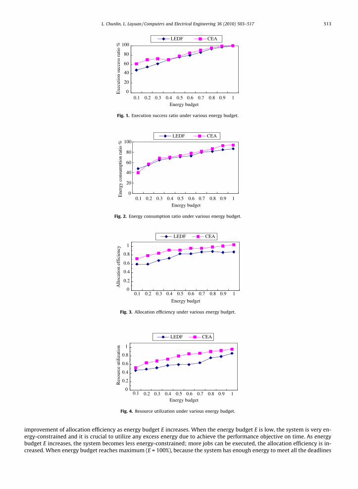
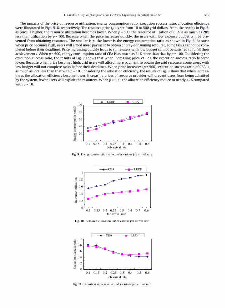
The impacts of the price on resource utilization, energy consumption ratio, execution success ratio, allocation efficiencywere illustrated in Figs. 5–8, respectively. The resource price (p) is set from 10 to 500 grid dollars. From the results in Fig. 5,as price is higher, the resource utilization becomes lower. When p = 500, the resource utilization of CEA is as much as 28%less than utilization by p = 100. Because when the price increases quickly, the users with low expense budget will be pre-vented from obtaining resources. The smaller is p, the lower is the energy consumption ratio as shown in Fig. 6. Becausewhen price becomes high, users will afford more payment to obtain energy-consuming resource, some tasks cannot be com-pleted before their deadlines. Price increasing quickly leads to some users with low budget cannot be satisfied to fulfill theirachievements. When p = 500, energy consumption ratio of CEA is as much as 34% more than that by p = 100. Considering theexecution success ratio, the results of Fig. 7 shows that when increasing price values, the execution success ratio becomelower. Because when price becomes high, grid users will afford more payment to obtain the grid resource, some users withlow budget will not complete tasks before their deadlines. When price increases (p = 500), execution success ratio of CEA isas much as 39% less than that with p = 10. Considering the allocation efficiency, the results of Fig. 8 show that when increas-ing p, the allocation efficiency become lower. Increasing prices of resource provider will prevent users from being admittedby the system, fewer users will exploit the resources. When p = 500, the allocation efficiency reduce to nearly 42% comparedwith p = 10.
0
20
40
60
80
100
Job arrival rate
Ene
rgy
cons
umpt
ion
ratio
%
LEDF CEA
0.1 0.15 0.2 0.25 0.3 0.4 0.5 0.6
Fig. 9. Energy consumption ratio under various job arrival rate.
0
0.2
0.4
0.6
0.8
1
Job arrival rate
Res
ourc
e ut
iliza
tion
CEA LEDF
0.1 0.15 0.2 0.25 0.3 0.4 0.5 0.6
Fig. 10. Resource utilization under various job arrival rate.
0
0.2
0.4
0.6
0.8
1
Job arrival rate
Exe
cutio
n su
cces
s ra
tio
CEA LEDF
0.1 0.15 0.2 0.25 0.3 0.4 0.5 0.6
Fig. 11. Execution success ratio under various job arrival rate.
0
0.2
0.4
0.6
0.8
1
0.1 0.15 0.2 0.25 0.3 0.4 0.5 0.6Job arrival rate
Allo
catio
n ef
fici
ency
CEA LEDF
Fig. 12. Allocation efficiency under various job arrival rate.
516 L. Chunlin, L. Layuan / Computers and Electrical Engineering 36 (2010) 503–517
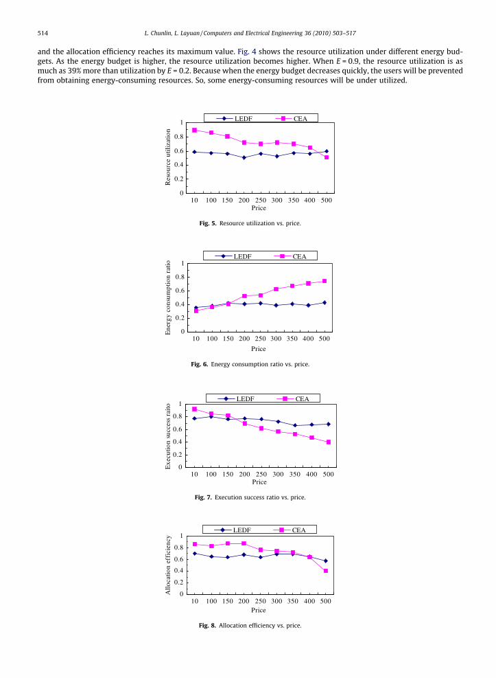
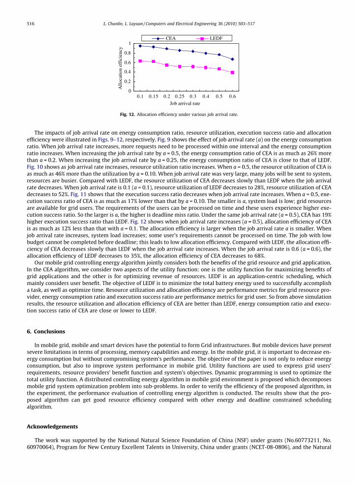
The impacts of job arrival rate on energy consumption ratio, resource utilization, execution success ratio and allocationefficiency were illustrated in Figs. 9–12, respectively. Fig. 9 shows the effect of job arrival rate (a) on the energy consumptionratio. When job arrival rate increases, more requests need to be processed within one interval and the energy consumptionratio increases. When increasing the job arrival rate by a = 0.5, the energy consumption ratio of CEA is as much as 26% morethan a = 0.2. When increasing the job arrival rate by a = 0.25, the energy consumption ratio of CEA is close to that of LEDF.Fig. 10 shows as job arrival rate increases, resource utilization ratio increases. When a = 0.5, the resource utilization of CEA isas much as 46% more than the utilization by a = 0.10. When job arrival rate was very large, many jobs will be sent to system,resources are busier. Compared with LEDF, the resource utilization of CEA decreases slowly than LEDF when the job arrivalrate decreases. When job arrival rate is 0.1 (a = 0.1), resource utilization of LEDF decreases to 28%, resource utilization of CEAdecreases to 52%. Fig. 11 shows that the execution success ratio decreases when job arrival rate increases. When a = 0.5, exe-cution success ratio of CEA is as much as 17% lower than that by a = 0.10. The smaller is a, system load is low; grid resourcesare available for grid users. The requirements of the users can be processed on time and these users experience higher exe-cution success ratio. So the larger is a, the higher is deadline miss ratio. Under the same job arrival rate (a = 0.5), CEA has 19%higher execution success ratio than LEDF. Fig. 12 shows when job arrival rate increases (a = 0.5), allocation efficiency of CEAis as much as 12% less than that with a = 0.1. The allocation efficiency is larger when the job arrival rate a is smaller. Whenjob arrival rate increases, system load increases; some user’s requirements cannot be processed on time. The job with lowbudget cannot be completed before deadline; this leads to low allocation efficiency. Compared with LEDF, the allocation effi-ciency of CEA decreases slowly than LEDF when the job arrival rate increases. When the job arrival rate is 0.6 (a = 0.6), theallocation efficiency of LEDF decreases to 35%, the allocation efficiency of CEA decreases to 68%.
Our mobile grid controlling energy algorithm jointly considers both the benefits of the grid resource and grid application.In the CEA algorithm, we consider two aspects of the utility function: one is the utility function for maximizing benefits ofgrid applications and the other is for optimizing revenue of resources. LEDF is an application-centric scheduling, whichmainly considers user benefit. The objective of LEDF is to minimize the total battery energy used to successfully accomplisha task, as well as optimize time. Resource utilization and allocation efficiency are performance metrics for grid resource pro-vider, energy consumption ratio and execution success ratio are performance metrics for grid user. So from above simulationresults, the resource utilization and allocation efficiency of CEA are better than LEDF, energy consumption ratio and execu-tion success ratio of CEA are close or lower to LEDF.
6. Conclusions
In mobile grid, mobile and smart devices have the potential to form Grid infrastructures. But mobile devices have presentsevere limitations in terms of processing, memory capabilities and energy. In the mobile grid, it is important to decrease en-ergy consumption but without compromising system’s performance. The objective of the paper is not only to reduce energyconsumption, but also to improve system performance in mobile grid. Utility functions are used to express grid users’requirements, resource providers’ benefit function and system’s objectives. Dynamic programming is used to optimize thetotal utility function. A distributed controlling energy algorithm in mobile grid environment is proposed which decomposesmobile grid system optimization problem into sub-problems. In order to verify the efficiency of the proposed algorithm, inthe experiment, the performance evaluation of controlling energy algorithm is conducted. The results show that the pro-posed algorithm can get good resource efficiency compared with other energy and deadline constrained schedulingalgorithm.
Acknowledgements
The work was supported by the National Natural Science Foundation of China (NSF) under grants (No.60773211, No.60970064), Program for New Century Excellent Talents in University, China under grants (NCET-08-0806), and the Natural

L. Chunlin, L. Layuan / Computers and Electrical Engineering 36 (2010) 503–517 517
Science Foundation of HuBei Province under Grant (No.2008CDB335). Any opinions, findings and conclusions are those of theauthors and do not necessarily reflect the views of the above agencies.
References
[1] Chu D, Humphrey M. Mobile OGSI.NET: grid computing on mobile devices. In: 5th IEEE/ACM international workshop on grid computing – GRID2004,Pittsburgh, PA; 8 November, 2004.
[2] Zhou Chi, Qian Dayou, Lee Hyunjeong. Utility-based routing in wireless ad hoc networks, In: 2004 IEEE international conference on mobile ad-hoc andsensor systems; 25–27 October 2004. p. 588–93.
[3] Huang Jen-Hung, Kao Yu-Fen. Price-based resource allocation strategies for wireless ad hoc networks with transmission rate and energy constraints.In: ICCCN 2007. Proceedings of the 16th international conference on computer communications and networks; 13–16 August 2007. p. 1065–70.
[4] Chen Lin, Leneutre Jean. A game theoretic framework of distributed power and rate control in IEEE 802.11 WLANs. IEEE J Sel Area Commun2008;26(7):1128–37.
[5] Alsalih Waleed, Akl Selim, Hassanein Hossam. Energy-aware task allocation over MANETs. In: Wireless and mobile computing, networking andcommunications, 2005 (WiMobapos, 2005). IEEE Press; 2005, p. 315–22.
[6] Chen Jing, Shen Hong, Tian Hui. Energy balanced data gathering in WSNs with grid topologies. In: Seventh international conference on grid andcooperative computing (GCC); 2008. p. 362–8.
[7] Shang L, Dick RP, Jha NK. An economics-based power-aware protocol for computation distribution in mobile ad-hoc networks. In: Proceedings of theIASTED international conference on parallel and distributed computing and systems; November 2002, p. 344–9.
[8] Park Eunjeong, Shin Heonshik, Kim Seung Jo. Selective grid access for energy-aware mobile computing. In: Indulska J, et al. editors, Proceedings of theUIC 2007, LNCS, vol. 4611; 2007, p. 798–807.
[9] Seshasayee Balasubramanian, Nathuji Ripal, Schwan Karsten. Energy-aware mobile service overlays: cooperative dynamic power management indistributed mobile systems. In: Fourth international conference on autonomic computing (ICAC’07). IEEE Press; 2007.
[10] Zong Ziliang, Qin Xiao. Energy-efficient scheduling for parallel applications running on heterogeneous clusters. In: International conference on parallelprocessing (ICPP 2007). IEEE Press; 2007.
[11] Huang Y, Mohapatra S, Venkatasubramanian N. An energy-efficient middleware for supporting multimedia services in mobile grid environments. In:IEEE International Conference on Information Technology; 2005.
[12] Kim Kyong Hoon, Buyya Rajkumar, Kim Jong. Power aware scheduling of bag-of-tasks applications with deadline constraints on DVS-enabled clusters.In: Proceedings of the seventh IEEE international symposium on cluster computing and the grid. Washington, DC, USA: IEEE Computer Society; 2007. p.541–8.
[13] Swaminathan V, Chakrabarty K. Real-time task scheduling for energy-aware embedded systems. J Franklin Inst 2001;338(9):729–50.[14] Khan Samee Ullah, Ahmad Ishfaq. A cooperative game theoretical technique for joint optimization of energy consumption and response time in
computational grids. IEEE Trans Parallel Distrib Syst 2009;20(3):346–60.[15] Katsaros Konstantinos, Polyzos George C. Evaluation of scheduling policies in a mobile grid architecture. In: SPECTS 2008. IEEE Press; 2008. p. 390–7.[16] Li Chunlin, Li Layuan. A distributed utility-based two level market solution for optimal resource scheduling in computational grid. Parallel Comput
2005;31(3–4):332–51.[17] Li Chunlin, Li Layuan. Multi economic agent interaction for optimizing the aggregate utility of grid users in computational grid. Appl Intell
2006;25(2):147–58.[18] Li Chunlin, Li Layuan. Utility based QoS optimisation strategy for multi-criteria scheduling on the grid. J Parallel Distrib Comput 2007;67(2):142–53.[19] Li Chunlin, Li Layuan. Joint QoS optimization for layered computational grid. Inform Sci 2007;177(15):3038–59.[20] Li Chunlin, Li Layuan. Agent framework to support computational grid. J Syst Software 2004;70(1–2):177–87.[21] Javasim, <http://javasim.ncl.ac.uk>.[22] Brite, <http://www.cs.bu.edu/brite>.[23] Wolski R, Plank J, Brevik J, Bryan T. Analyzing market-based resource allocation strategies for the computational grid. Int J High-Perform Comput Appl
2001;15(3):258–81.[24] Ernemann C. Economic scheduling in grid computing. Proceeding of the eighth international workshop job scheduling strategies for parallel
processing. Lect Notes Comput Sci 2002:128–52.


![[Mystical Signs] - Compromising Positions](https://img.dokumen.tips/doc/110x75/577c85f91a28abe054bf4b96/mystical-signs-compromising-positions.jpg)