Embed Size (px)
Citation preview
The University of Newcastle
ELEC4410
Control Systems Design
Lecture 23: Optimal LQG Control
Julio H. Braslavsky
School of Electrical Engineering and Computer Science
The University of Newcastle
Lecture 23: Optimal LQG Control – p. 1
The University of Newcastle
Outline
LQG Control
LQG Control for Disturbance Rejection
Lecture 23: Optimal LQG Control – p. 2
The University of Newcastle
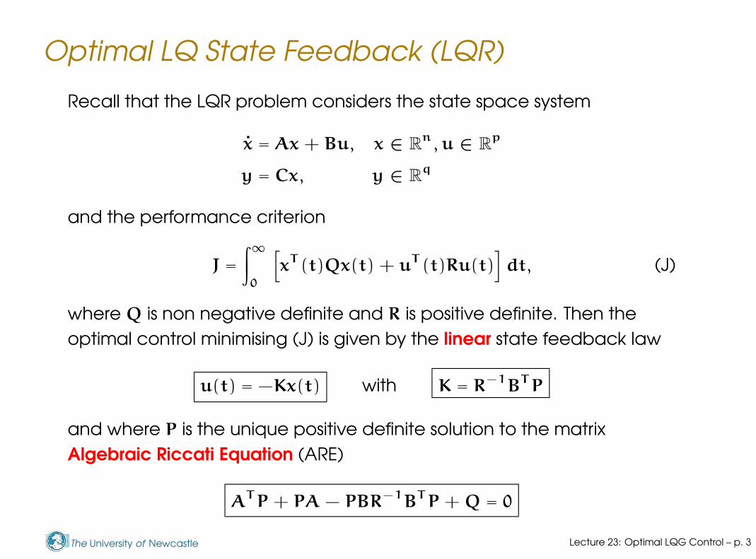
Optimal LQ State Feedback (LQR)
Recall that the LQR problem considers the state space system
x = Ax + Bu, x ∈ Rn, u ∈ R
p
y = Cx, y ∈ Rq
and the performance criterion
J =
∫∞
0
h
xT(t)Qx(t) + u
T(t)Ru(t)
i
dt, (J)
where Q is non negative definite and R is positive definite. Then the
optimal control minimising (J) is given by the linear state feedback law
u(t) = −Kx(t) with K = R−1
BTP
and where P is the unique positive definite solution to the matrix
Algebraic Riccati Equation (ARE)
ATP + PA − PBR
−1B
TP + Q = 0
Lecture 23: Optimal LQG Control – p. 3
The University of Newcastle
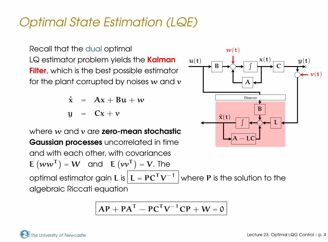
Optimal State Estimation (LQE)
Recall that the dual optimal
A − LC
B
A
∫ x(t)C
u(t)
∫L
B
x(t)
y(t)
w(t)
v(t)
Observer
LQ estimator problem yields the Kalman
Filter, which is the best possible estimator
for the plant corrupted by noises w and v
x = Ax + Bu + w
y = Cx + v
where w and v are zero-mean stochastic
Gaussian processes uncorrelated in time
and with each other, with covariances
E`
wwT´
= W and E`
vvT´
= V. The
optimal estimator gain L is L = PCTV
−1 where P is the solution to the
algebraic Riccati equation
AP + PAT
− PCTV
−1CP + W = 0
Lecture 23: Optimal LQG Control – p. 4
The University of Newcastle
Linear Quadratic Gaussian (LQG) Control
LQG is the optimal controller obtained as the combination of
Lecture 23: Optimal LQG Control – p. 5
The University of Newcastle
Linear Quadratic Gaussian (LQG) Control
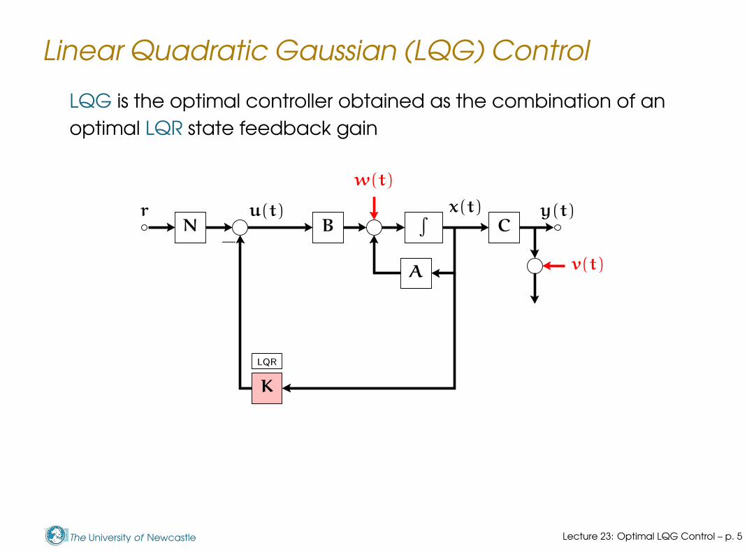
LQG is the optimal controller obtained as the combination of an
optimal LQR state feedback gain
B
A
∫ x(t)CN
−
u(t)
K
y(t)r
w(t)
v(t)
LQR
Lecture 23: Optimal LQG Control – p. 5
The University of Newcastle
Linear Quadratic Gaussian (LQG) Control
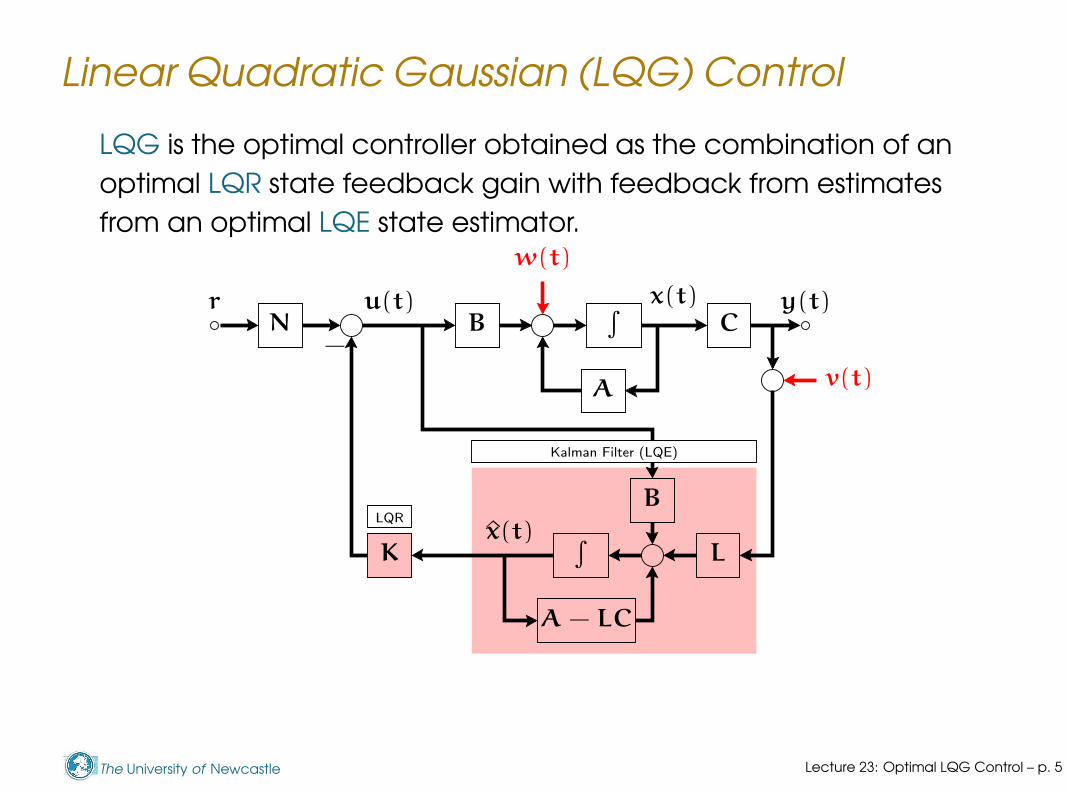
LQG is the optimal controller obtained as the combination of an
optimal LQR state feedback gain with feedback from estimates
from an optimal LQE state estimator.
A − LC
B
A
∫ x(t)CN
−
u(t)
∫L
B
Kx(t)
y(t)r
w(t)
v(t)
Kalman Filter (LQE)
LQR
Lecture 23: Optimal LQG Control – p. 5
The University of Newcastle
Linear Quadratic Gaussian (LQG) Control
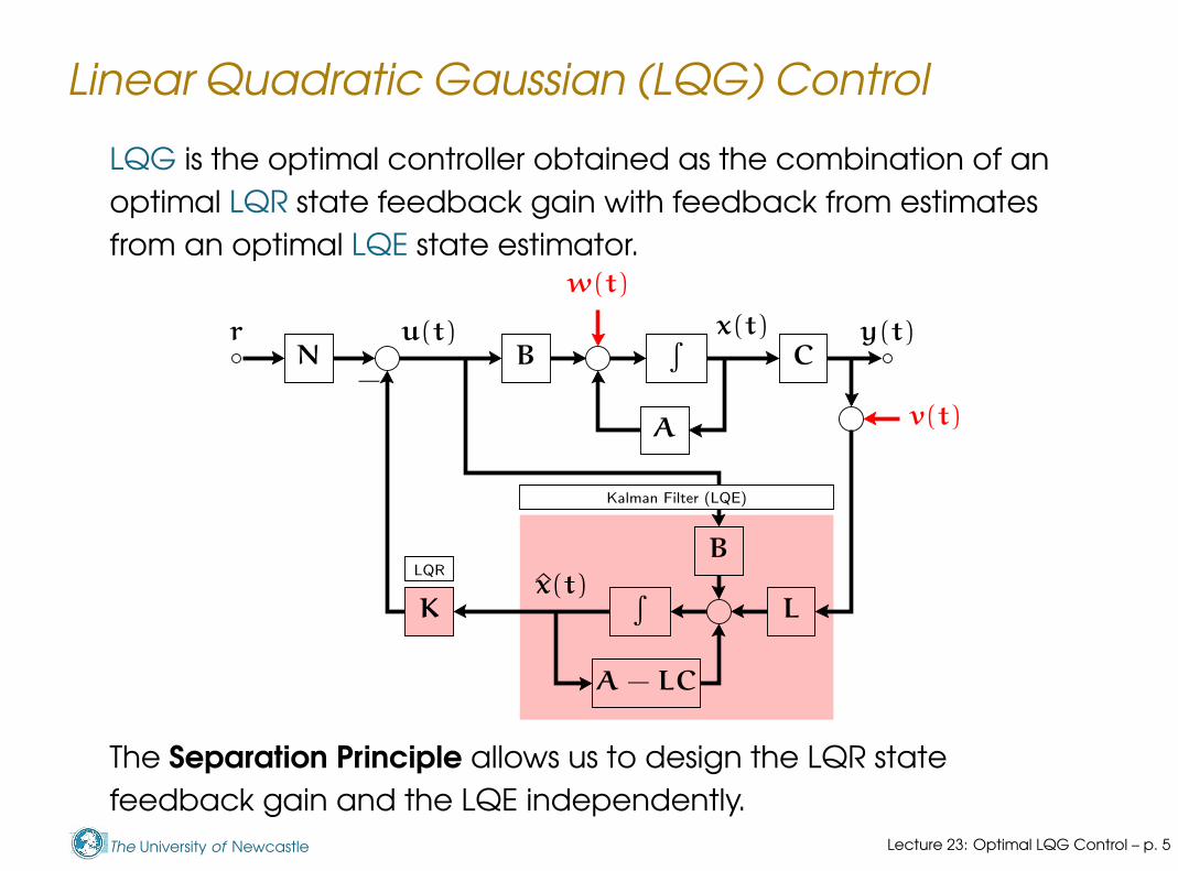
LQG is the optimal controller obtained as the combination of an
optimal LQR state feedback gain with feedback from estimates
from an optimal LQE state estimator.
A − LC
B
A
∫ x(t)CN
−
u(t)
∫L
B
Kx(t)
y(t)r
w(t)
v(t)
Kalman Filter (LQE)
LQR
The Separation Principle allows us to design the LQR state
feedback gain and the LQE independently.
Lecture 23: Optimal LQG Control – p. 5
The University of Newcastle
LQR, LQE and Separation Principle
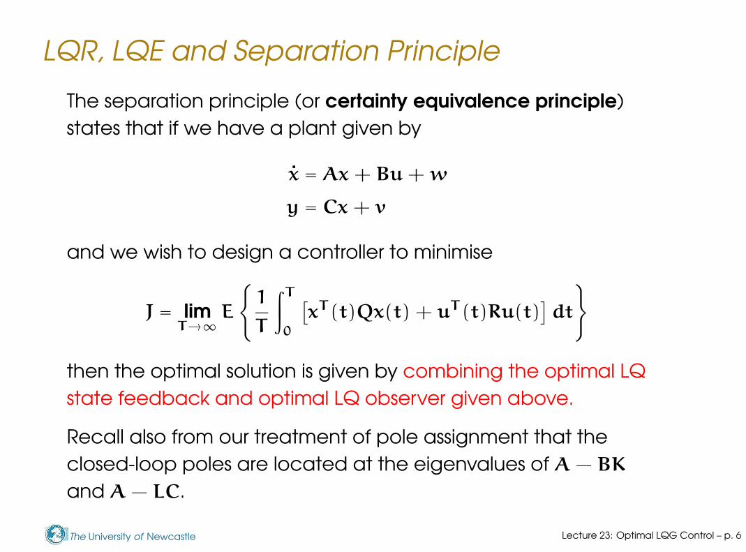
The separation principle (or certainty equivalence principle)
states that if we have a plant given by
x = Ax + Bu + w
y = Cx + v
and we wish to design a controller to minimise
J = limT→∞
E
{1
T
∫T
0
[
xT (t)Qx(t) + uT (t)Ru(t)]
dt
}
then the optimal solution is given by combining the optimal LQ
state feedback and optimal LQ observer given above.
Recall also from our treatment of pole assignment that the
closed-loop poles are located at the eigenvalues of A − BK
and A − LC.
Lecture 23: Optimal LQG Control – p. 6
The University of Newcastle
LQG Design Remarks
The combined controller including an LQR (optimal linear
quadratic regulator) and LQE (optimal linear quadratic
estimator) is usually called the Linear Quadratic Gaussian
(LQG) controller.
Lecture 23: Optimal LQG Control – p. 7
The University of Newcastle
LQG Design Remarks
The combined controller including an LQR (optimal linear
quadratic regulator) and LQE (optimal linear quadratic
estimator) is usually called the Linear Quadratic Gaussian
(LQG) controller.
LQG can be used as a simple tool to get a ball-park
controller with reasonable performance. Just as with pole
assignment the plant must be augmented if features such as
integral action are desired.
There are also sophisticated design strategies based on LQG.
These address not only intricate dynamics (e.g. resonant
systems or interactions in multivariable systems) but also
ensure the resultant design has suitable robustness
properties. Such strategies are beyond the scope of this
course, but the book “Multivariable Feedback Design” by
J.M. Maciejowski (Addison Wesley, 1989) is recommended.
Lecture 23: Optimal LQG Control – p. 7
The University of Newcastle
LQG Control for Disturbance Rejection
As an LQG control example we consider an application of
disturbance rejection by the Internal Model Principle (from Bay,
Linear State Space Systems, McGraw-Hill, 1999).
Lecture 23: Optimal LQG Control – p. 8
The University of Newcastle
LQG Control for Disturbance Rejection
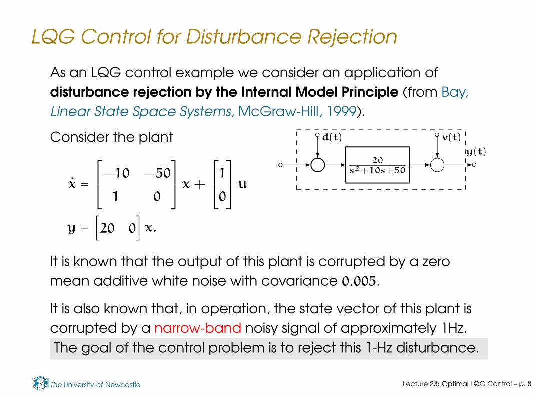
As an LQG control example we consider an application of
disturbance rejection by the Internal Model Principle (from Bay,
Linear State Space Systems, McGraw-Hill, 1999).
b
b b
bj j- - --??
y(t)
v(t)d(t)
20s2+10s+50
Consider the plant
x =
−10 −50
1 0
x +
1
0
u
y =[
20 0
]
x.
It is known that the output of this plant is corrupted by a zero
mean additive white noise with covariance 0.005.
It is also known that, in operation, the state vector of this plant is
corrupted by a narrow-band noisy signal of approximately 1Hz.
The goal of the control problem is to reject this 1-Hz disturbance.
Lecture 23: Optimal LQG Control – p. 8
The University of Newcastle
LQG Control for Disturbance Rejection
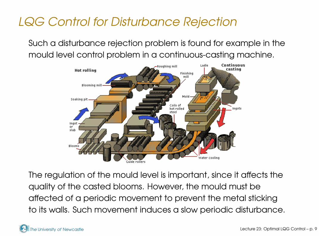
Such a disturbance rejection problem is found for example in the
mould level control problem in a continuous-casting machine.
The regulation of the mould level is important, since it affects the
quality of the casted blooms. However, the mould must be
affected of a periodic movement to prevent the metal sticking
to its walls. Such movement induces a slow periodic disturbance.
Lecture 23: Optimal LQG Control – p. 9
The University of Newcastle
LQG Control for Disturbance Rejection
A basic principle we will follow is that in order to be able to reject
a disturbance, or track a reference, we need to incorporate a
model of the disturbance in the controller. This is known as the
Internal Model Principle.
Lecture 23: Optimal LQG Control – p. 10
The University of Newcastle
LQG Control for Disturbance Rejection
A basic principle we will follow is that in order to be able to reject
a disturbance, or track a reference, we need to incorporate a
model of the disturbance in the controller. This is known as the
Internal Model Principle.
The Internal Model Principle establishes that in order to reject a
disturbance, the system must include a model of the disturbance,
if available.
One familiar example of disturbance rejection (and reference
tracking) based on the Internal Model Principle is the integral
action in state feedback: In order to reject constant
disturbances we augment their model (an integrator) into the
plant.
Lecture 23: Optimal LQG Control – p. 10
The University of Newcastle
LQG Control for Disturbance Rejection
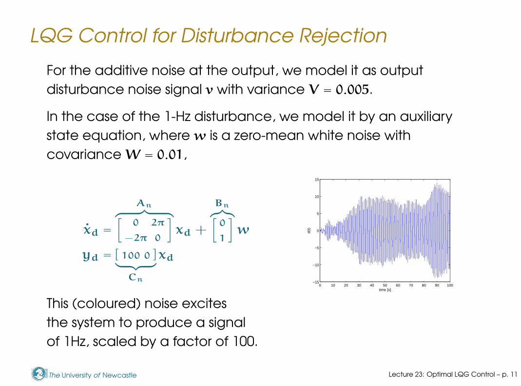
For the additive noise at the output, we model it as output
disturbance noise signal v with variance V = 0.005.
In the case of the 1-Hz disturbance, we model it by an auxiliary
state equation, where w is a zero-mean white noise with
covariance W = 0.01,
0 10 20 30 40 50 60 70 80 90 100−15
−10
−5
0
5
10
15
d(t)
time [s]
xd =
An
︷ ︸︸ ︷[
0 2π
−2π 0
]
xd +
Bn
︷︸︸︷[
0
1
]
w
yd = [ 100 0 ]︸ ︷︷ ︸
Cn
xd
This (coloured) noise excites
the system to produce a signal
of 1Hz, scaled by a factor of 100.
Lecture 23: Optimal LQG Control – p. 11
The University of Newcastle
LQG Control for Disturbance Rejection
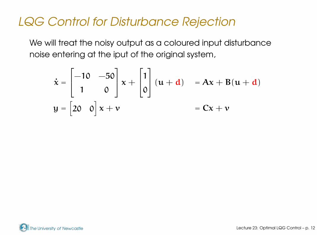
We will treat the noisy output as a coloured input disturbance
noise entering at the iput of the original system,
x =
−10 −50
1 0
x +
1
0
(u + d) = Ax + B(u + d)
y =[
20 0
]
x + v = Cx + v
Lecture 23: Optimal LQG Control – p. 12

The University of Newcastle
LQG Control for Disturbance Rejection
We will treat the noisy output as a coloured input disturbance
noise entering at the iput of the original system,
x =
−10 −50
1 0
x +
1
0
(u + d) = Ax + B(u + d)
y =[
20 0
]
x + v = Cx + v
We will design a Kalman filter to reject this disturbance. For the
design we combine plant and disturbance in the augmented
plant (Aa, Ba, Ca, Da):
x
xd
=
A B
0 An
x
xd
+
B
0
u +
0
Bn
w
y =[
C 0
]
x
xd
+ v
Lecture 23: Optimal LQG Control – p. 12
The University of Newcastle
LQG Control for Disturbance Rejection
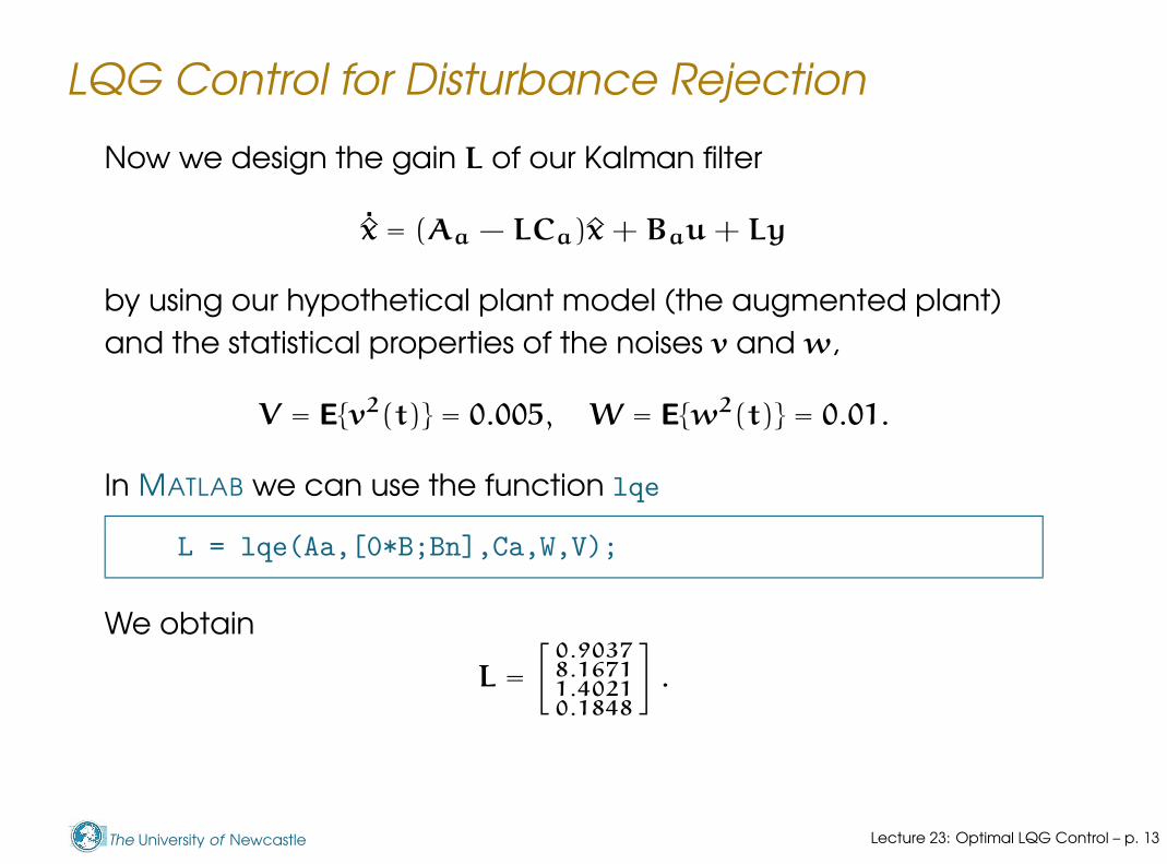
Now we design the gain L of our Kalman filter
˙x = (Aa − LCa)x + Bau + Ly
by using our hypothetical plant model (the augmented plant)
and the statistical properties of the noises v and w,
V = E{v2(t)} = 0.005, W = E{w2(t)} = 0.01.
In MATLAB we can use the function lqe
L = lqe(Aa,[0*B;Bn],Ca,W,V);
We obtain
L =
[
0.90378.16711.40210.1848
]
.
Lecture 23: Optimal LQG Control – p. 13
The University of Newcastle
LQG Control for Disturbance Rejection
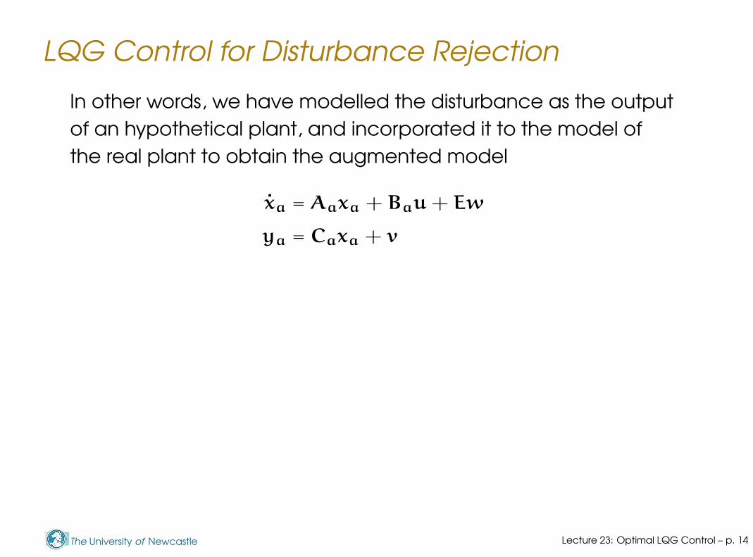
In other words, we have modelled the disturbance as the output
of an hypothetical plant, and incorporated it to the model of
the real plant to obtain the augmented model
xa = Aaxa + Bau + Ew
ya = Caxa + v
Lecture 23: Optimal LQG Control – p. 14
The University of Newcastle
LQG Control for Disturbance Rejection
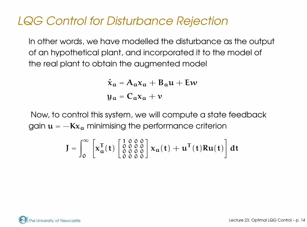
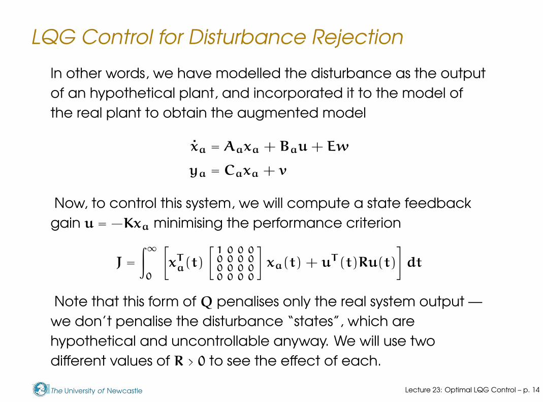
In other words, we have modelled the disturbance as the output
of an hypothetical plant, and incorporated it to the model of
the real plant to obtain the augmented model
xa = Aaxa + Bau + Ew
ya = Caxa + v
Now, to control this system, we will compute a state feedback
gain u = −Kxa minimising the performance criterion
J =
∫∞
0
[
xTa(t)
[
1 0 0 00 0 0 00 0 0 00 0 0 0
]
xa(t) + uT (t)Ru(t)
]
dt
Lecture 23: Optimal LQG Control – p. 14
The University of Newcastle
LQG Control for Disturbance Rejection
In other words, we have modelled the disturbance as the output
of an hypothetical plant, and incorporated it to the model of
the real plant to obtain the augmented model
xa = Aaxa + Bau + Ew
ya = Caxa + v
Now, to control this system, we will compute a state feedback
gain u = −Kxa minimising the performance criterion
J =
∫∞
0
[
xTa(t)
[
1 0 0 00 0 0 00 0 0 00 0 0 0
]
xa(t) + uT (t)Ru(t)
]
dt
Note that this form of Q penalises only the real system output —
we don’t penalise the disturbance “states”, which are
hypothetical and uncontrollable anyway. We will use two
different values of R > 0 to see the effect of each.
Lecture 23: Optimal LQG Control – p. 14
The University of Newcastle
LQG Control for Disturbance Rejection
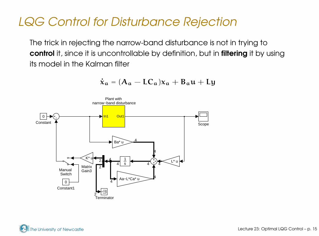
The trick in rejecting the narrow-band disturbance is not in trying to
control it, since it is uncontrollable by definition, but in filtering it by using
its model in the Kalman filter
xa = (Aa − LCa)xa + Bau + Ly
Terminator
Scope
In1 Out1
Plant with narrow−band disturbance
K* u
MatrixGain3
Aa−L*Ca* u
L* u
Ba* u
Manual Switch
1s
Demux
0
Constant1
0
Constant
4
4
4
44
44 4
2
2
2
Lecture 23: Optimal LQG Control – p. 15
The University of Newcastle
LQG Control for Disturbance Rejection
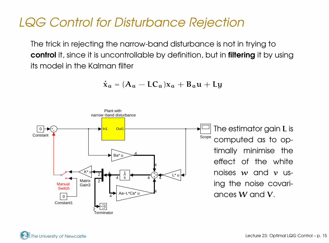
The trick in rejecting the narrow-band disturbance is not in trying to
control it, since it is uncontrollable by definition, but in filtering it by using
its model in the Kalman filter
xa = (Aa − LCa)xa + Bau + Ly
Terminator
Scope
In1 Out1
Plant with narrow−band disturbance
K* u
MatrixGain3
Aa−L*Ca* u
L* u
Ba* u
Manual Switch
1s
Demux
0
Constant1
0
Constant
4
4
4
44
44 4
2
2
2
The estimator gain L is
computed as to op-
timally minimise the
effect of the white
noises w and v us-
ing the noise covari-
ances W and V.
Lecture 23: Optimal LQG Control – p. 15
The University of Newcastle
LQG Control for Disturbance Rejection
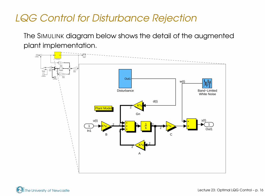
The SIMULINK diagram below shows the detail of the augmented
plant implementation.
Terminator
In1 Out1
Subsystem
Scope
K*u
MatrixGain3
Aa−L*Ca* u
MatrixGain2
L* u
MatrixGain1
K*u
MatrixGain
Manual Switch
1s
Integrator
Demux
0
Constant1
0
Constant
4
4
4
4
4
4
44 4
2
2
2
Plant Model
y(t)
w(t)
d(t)
u(t)1
Out1
1s
K*u
Gn
Out1
Disturbance
K*u
C
Band−LimitedWhite Noise
K*u
B
K*u
A
1
In1
2
2
2
2
2
22
2
2
Lecture 23: Optimal LQG Control – p. 16
The University of Newcastle
LQG Control for Disturbance Rejection
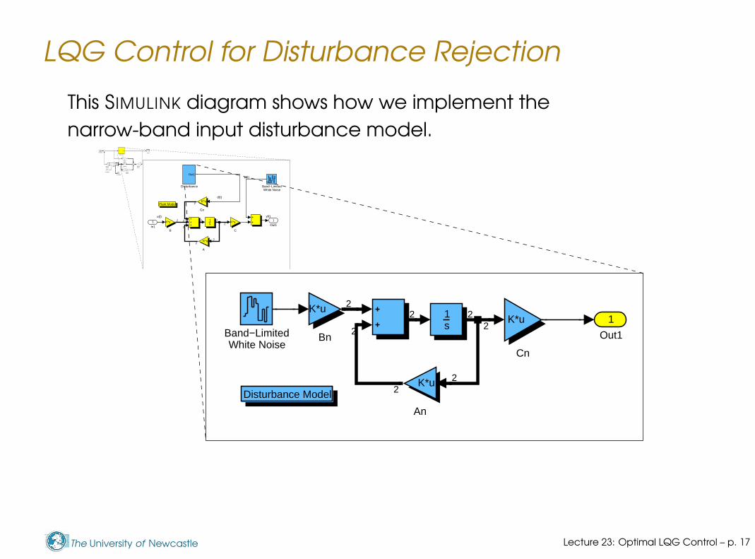
This SIMULINK diagram shows how we implement the
narrow-band input disturbance model.
Terminator
In1 Out1
Subsystem
Scope
K*u
MatrixGain3
Aa−L*Ca* u
MatrixGain2
L* u
MatrixGain1
K*u
MatrixGain
Manual Switch
1s
Integrator
Demux
0
Constant1
0
Constant
4
4
4
4
4
4
44 4
2
2
2
Plant Model
y(t)
w(t)
d(t)
u(t)1
Out1
1s
K*u
Gn
Out1
Disturbance
K*u
C
Band−LimitedWhite Noise
K*u
B
K*u
A
1
In1
2
2
2
2
2
22
2
2
Disturbance Model
1
Out1
1s
K*u
Cn
K*u
BnBand−LimitedWhite Noise
K*u
An
2
2
2
2
22
2
Lecture 23: Optimal LQG Control – p. 17
The University of Newcastle
LQG Control for Disturbance Rejection
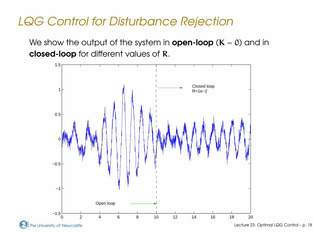
We show the output of the system in open-loop (K = 0) and in
closed-loop for different values of R.
0 2 4 6 8 10 12 14 16 18 20−1.5
−1
−0.5
0
0.5
1
1.5
Closed loopR=1e−2
Open loop
Lecture 23: Optimal LQG Control – p. 18

The University of Newcastle
LQG Control for Disturbance Rejection
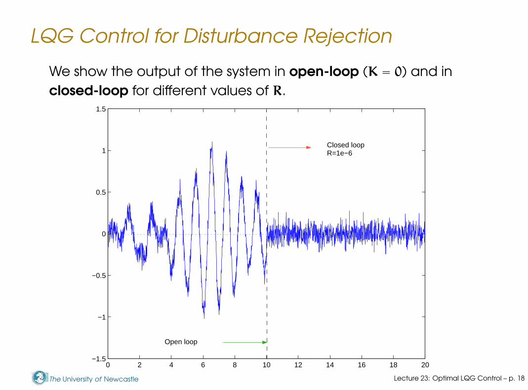
We show the output of the system in open-loop (K = 0) and in
closed-loop for different values of R.
0 2 4 6 8 10 12 14 16 18 20−1.5
−1
−0.5
0
0.5
1
1.5
Closed loopR=1e−4
Open loop
Lecture 23: Optimal LQG Control – p. 18
The University of Newcastle
LQG Control for Disturbance Rejection
We show the output of the system in open-loop (K = 0) and in
closed-loop for different values of R.
0 2 4 6 8 10 12 14 16 18 20−1.5
−1
−0.5
0
0.5
1
1.5
Closed loopR=1e−6
Open loop
Lecture 23: Optimal LQG Control – p. 18
The University of Newcastle
LQG Control for Disturbance Rejection
For values of the control weight R < 10−4 there is no
significant improvement in the response, because the system
has a “floor” noise level due to the measurement noise v
(which we will not be able to remove from the output).
However, we could effectively improve the response in
removing the narrow band disturbance.
This is a way of dealing with disturbances in the observer
rather than in the feedback control, as we did in the integral
action scheme we learned previously.
Lecture 23: Optimal LQG Control – p. 19
The University of Newcastle
LQG Control for Disturbance Rejection
10−1
100
101
102
103
104
−200
−150
−100
−50
0
50
Mag
nitu
de (
dB)
Bode Diagram
Frequency (rad/sec)
Open Loop
R=10−2
R=10−4
R=10−6
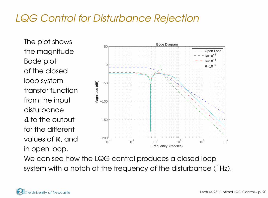
The plot shows
the magnitude
Bode plot
of the closed
loop system
transfer function
from the input
disturbance
d to the output
for the different
values of R, and
in open loop.
We can see how the LQG control produces a closed loop
system with a notch at the frequency of the disturbance (1Hz).
Lecture 23: Optimal LQG Control – p. 20
The University of Newcastle
Final Remarks on LQG
Of course, we can incorporate in our LQG design integral
action, by augmenting the plant with the integral of the
tracking error. We should then be careful in selecting Q so
that we penalise the tracking error and not the state that is
suppose to track a reference.
Lecture 23: Optimal LQG Control – p. 21
The University of Newcastle
Final Remarks on LQG
Of course, we can incorporate in our LQG design integral
action, by augmenting the plant with the integral of the
tracking error. We should then be careful in selecting Q so
that we penalise the tracking error and not the state that is
suppose to track a reference.
Since LQG is a state feedback controller in combination with
a state estimator, we can incorporate antiwindup as we did
for state feedback with integral action.
LQG is one of the most basic and important tools in the
control engineer’s toolbox. For a state space models, it
constitutes in most cases the first choice for control design.
LQG is generally not robust, but it will almost always give
good results when the model of the system is reasonably
accurate.
Lecture 23: Optimal LQG Control – p. 21