Control of dipolar collisions in the quantum regime

by

Marcio H. G. de Miranda

B.Sc., Federal University of Pernambuco, 2002

M.Sc., Federal University of Pernambuco, 2004

M.A., University of Colorado at Boulder, 2008

A thesis submitted to the

Faculty of the Graduate School of the

University of Colorado in partial fulfillment

of the requirements for the degree of

Doctor of Philosophy

Department of Physics

2010

This thesis entitled:Control of dipolar collisions in the quantum regime

written by Marcio H. G. de Mirandahas been approved for the Department of Physics

Dr. Jun Ye

Dr. Deborah S. Jin

Date

The final copy of this thesis has been examined by the signatories, and we find that boththe content and the form meet acceptable presentation standards of scholarly work in the

above mentioned discipline.

iii

Miranda, Marcio H. G. de (Ph.D., Physics)

Control of dipolar collisions in the quantum regime

Thesis directed by Professor Dr. Jun Ye

The preparation of ultracold polar molecular gases close to quantum degeneracy opens

novel research prospects ranging from dipolar quantum many-body physics to ultracold

chemistry. With a near quantum degenerate gas of fermionic 40K87Rb polar molecules,

this thesis presents studies on dipolar collision and chemical reaction dynamics, exhibiting

long range interactions and spatial anisotropy. With full control over the internal quantum

state of the molecules, we show how quantum statistics of the molecule determines the rate

of chemical reactivity in the limit of vanishing collisional energy. Manipulating the interac-

tion potential between indistinguishable polar molecules by means of control over the dipole

moment of the molecules, we study the dramatic influence of the dipolar interaction on the

chemical reaction rate. In particular, we show that the chemical reaction rate increases

steeply with the dipole moment following a characteristic power law. This power law reflects

the long-range character of the dipole-dipole interaction. Studies on thermodynamics in the

molecular quantum gas reveal the anisotropic properties of the dipolar interaction. Finally,

combining control over the molecular dipole moment and the dimensionality of the spatial

confinement, we suppress inelastic collisions between polar molecules by up to two orders

of magnitude. The suppression of inelastic collisions is achieved by changing the geometry

of the confinement from three-dimensional to two-dimensional optical trapping. With the

combination of a sufficiently tight 2D confinement and Fermi statistics of the molecules,

two polar molecules approach each other only in a “side-by-side” collision, where the in-

elastic collisions are suppressed by the repulsive dipole-dipole interaction. This suppression

requires quantum state control of internal (electronic, vibrational, rotational and hyperfine

states) and external (harmonic oscillator levels of the optical lattice) degrees of freedom of

iv

the molecules. This is a fundamental advance in stabilizing a polar molecular gas for future

applications in quantum many-body systems.

Dedication

To my mother Leda, to my brother Marcelo and to my dear wife Fabiana for all love

and support.

vi

Acknowledgements

To be a physicist is not an easy thing. If you want to be a fully realized physicist one

day, you have to go through a Ph.D. program, for most of the average people. I chose to

follow this path in 1998 when I started as a student in the Federal University of Pernambuco

in my home town Recife. After spending 4 years to get bachelors and 2 years to get my

masters, I decided to do a Ph.D. when my application was accepted at the University of

Colorado at Boulder.

My Ph.D. work would be impossible without help of many people. I will start by

thanking Jun Ye for giving me the chance to work in his lab, for providing such an amazing

scientific environment, and for being on my side in all decisive moments. I thank Deborah

Jin for her attention and patience. I thank John Bohn for his patience and for answering my

dumb questions with a good mood. Thanks to Ana Maria Rey for stimulating discussions.

Thanks to John Hall for providing a stable laser source and lots of nice conversations about

lasers, physics, and life in general.

Thanks to Seth Foreman (“A” as in America), Daren Hudson, Michael Thorpe, Matt

Stowe, and Thomas Schibili for interesting discussions and frequency comb secrets that they

shared with me.

Thanks to the KRb group that I was part of. Thanks to Avi Pe’er who is an incredibly

patient person, very sharp and fun to work with. Thanks to Silke Ospelkaus for all she

taught me about cold atoms and molecules and for all that she did for me. Silke is the

advisor that any student would want to have. Thanks to Kang-Kuen Ni who taught me so

vii

much and sided with me most of the time despite of some disagreements. Thanks to Dajun

Wang (“Dajunio”) who is a hard working and sharp scientist. Thanks to Brian Neyenhuis

who is a very sharp guy and patient. Thanks to my French friend Amodsen Chotia who

is smart, has a nice sense of humor, and was a pleasure to work with. Thanks to another

French friend Goulven Quemener (Goulvinho “vote em mim”) for many good discussions

and explanations, for his theoretical support, and for his nice sense of humor with no French

accent. Thanks to Steve Moses who is going to be in charge of our frequency comb from

now on and who is also an excellent reinforcement for our group.

Thanks to my frequency comb friends Dylon Yost, Kevin Cossel, Travis Briels, Tici-

jana Ban, Thomas Allison, Aleksandra Matyba, Arman Cingoz, Florian Adler, and Piotr

Maslowski.

Thanks to my Sr friends Sebastian Blatt, Andrew Ludlow, Martin Boyd, Matt Swal-

lows, Travis Nicholson, Michael Martin, Michael Bishof, Gretchen Campbell, Tanya Zelev-

inzky, Thomas Zanon, Jan Thomsen, Yige Lin, Ben Bloom, and Jason Williams.

Thanks to my OH friends Brian Sawyer, Benjamin Stuhl, Eng Hiang Yeo, Matthew

Hummon, and Yong Xia.

Thanks to my friends from theory and soccer games such as Murray Holland, Javier

Von Stecher, Dominic Meiser, Brandon Peden, David Tieri, and Ron Pepino.

Thanks to the electronic shop staff Terry Brown (the master Yoda of microwave elec-

tronics), James Fung-A-Fat, Michael J. Whitmore, David J. Tegart, Carl Sauer and Paul

Beckingham for the excellent development and support with electronics.

Thanks also to J.R. Raith, Michael Page and Alan Dunwell for the excellent support

on computers.

Thanks to the machine shop staff Hans Green, Kim R. Hagen, Paul Ariel, Todd R.

Asnicar, Thomas P. Foote, Blaine P. Horner, Tracy Keep and David Alchenberger for high

quality of technical assistance.

Thanks to the supply office staff Jeff Sauter, Brian Lynch, Randall Holliness, and

viii

William Blue for providing such efficient support. Thanks to Diana Moreland and Krista

Beck for being so organized and helpful. Thanks to Agnieska Lynch for taking care of

financial paper work. Thanks to Jeanne M. Nijhowne for her efficient work and kindness.

Thanks to my friends Fan-Chi Lin, Yu-Li Liang, Oliver Lin, Ricardo Jimenes, Sungsoo

Choi, Eduardo Calleja, Quan Zhang and Qing Li, Max Brown, Shannon Sankar, Chester

Rubbo, and Qing Chao.

Thanks to Mike Dubson for help me with my comps II exam.

Thanks to my my dear Brazilian friends Paulo Berton, Leila Grieger, Helena Berton,

Doris Berton, Felipe Nievinsky, Giovana Vazatta, Jose D’Incao, Valeria Gabarra, Eloisa

D’Incao, Nick McCulloch (the one who has a Brazilian spirit) and Daiana McCulloch for

being so entertaining, nice and extremely helpful in hard times.

Thanks to professor Lucio Hora Acioli for assisting me with my masters and helping

me come to JILA.

Thanks to my mother Leda and to my brother Marcelo for their love, dedication, care

and sacrifice that they did in order to raise me like a honest, educated and hard working

person. Thanks to my dear wife Fabiana for all her love, patience, sacrifice, care and for

being so understanding when I had to spend so much time working and not with her.

Thanks to CAPES and Fulbright for financial support.

Contents

Chapter

1 Introduction 1

1.1 From ultracold atoms to ultracold molecules . . . . . . . . . . . . . . . . . . 1

1.2 Dipolar interactions . . . . . . . . . . . . . . . . . . . . . . . . . . . . . . . . 4

1.3 Overview of this thesis . . . . . . . . . . . . . . . . . . . . . . . . . . . . . . 5

1.4 Outline of the thesis . . . . . . . . . . . . . . . . . . . . . . . . . . . . . . . 7

2 Experimental Apparatus 9

2.1 From ultracold K and Rb atoms to ultracold ground-state molecules . . . . . 10

2.1.1 Preparation of a near quantum-degenerate mixture of 40K and 87Rb 10

2.1.2 Feshbach molecule creation . . . . . . . . . . . . . . . . . . . . . . . . 11

2.1.3 Two-photon coherent transfer - STIRAP . . . . . . . . . . . . . . . . 12

2.1.4 Preparation of ground-state polar molecules . . . . . . . . . . . . . . 23

2.2 Essential manipulation techniques for ground-state polar molecules . . . . . 26

2.2.1 Electric dipole moment of the molecules . . . . . . . . . . . . . . . . 27

2.3 Tuning the geometry of the external confinement - 1D Optical Lattice . . . . 29

3 Dipolar 40K87Rb Molecules in 3D geometry 32

3.1 Bimolecular chemical reactions at ultracold temperature . . . . . . . . . . . 33

3.2 The role of quantum statistics in determining the chemical reaction rate . . . 34

3.3 The experimental system . . . . . . . . . . . . . . . . . . . . . . . . . . . . . 35

x

3.4 Bimolecular chemical reactions at vanishing dipole moment . . . . . . . . . . 36

3.4.1 p-wave collisions . . . . . . . . . . . . . . . . . . . . . . . . . . . . . 36

3.4.2 s-wave collisions . . . . . . . . . . . . . . . . . . . . . . . . . . . . . . 41

3.5 Dipolar collisions with ultracold 40K87Rb in 3D geometry . . . . . . . . . . . 42

3.5.1 Dipoles and chemical reactions . . . . . . . . . . . . . . . . . . . . . . 42

3.5.2 The experiment . . . . . . . . . . . . . . . . . . . . . . . . . . . . . . 44

3.5.3 Controlling chemical reactions by means of the dipole moment of the

molecules . . . . . . . . . . . . . . . . . . . . . . . . . . . . . . . . . 44

3.5.4 Thermodynamics of dipolar collisions . . . . . . . . . . . . . . . . . . 48

3.5.5 Anisotropy of heating . . . . . . . . . . . . . . . . . . . . . . . . . . . 49

4 Polar Molecules in an 1D Optical Lattice: Going to 2D Geometry 54

4.1 Atoms in an one-dimensional optical lattice . . . . . . . . . . . . . . . . . . 55

4.1.1 Optical dipole traps for neutral atoms and molecules . . . . . . . . . 55

4.1.2 One-dimensional optical lattice . . . . . . . . . . . . . . . . . . . . . 57

4.1.3 Experimental realization of a 1D optical lattice . . . . . . . . . . . . 59

4.1.4 Quantum mechanical description of a particle confined in a periodic

potential: Bloch bands . . . . . . . . . . . . . . . . . . . . . . . . . . 60

4.2 Characterizing the optical lattice . . . . . . . . . . . . . . . . . . . . . . . . 65

4.2.1 Measuring the trapping frequencies by parametric heating . . . . . . 65

4.2.2 Kapitza-Dirac Scattering . . . . . . . . . . . . . . . . . . . . . . . . . 67

4.3 Loading atoms into the optical lattice . . . . . . . . . . . . . . . . . . . . . . 69

4.3.1 Loading atoms in the optical lattice . . . . . . . . . . . . . . . . . . . 72

4.4 Probing the quasimomentum distribution of atoms in optical lattices. . . . . 74

4.5 40K87Rb molecules in the optical lattice . . . . . . . . . . . . . . . . . . . . . 79

5 Suppression of Inelastic Collisions in 2D geometry 85

5.1 Chemical Reaction Rates and Stereodynamics . . . . . . . . . . . . . . . . . 86

xi

5.2 Collisions between Polar Molecules in Quasi-2D Geometry . . . . . . . . . . 87

5.3 Band Mapping of Molecules . . . . . . . . . . . . . . . . . . . . . . . . . . . 90

5.4 Suppression of Inelastic Collisions in the Optical Lattice . . . . . . . . . . . 95

6 Conclusion and Future Work 103

6.1 Conclusion . . . . . . . . . . . . . . . . . . . . . . . . . . . . . . . . . . . . . 103

6.2 Future work . . . . . . . . . . . . . . . . . . . . . . . . . . . . . . . . . . . . 103

Bibliography 105

xii

Figures

Figure

1.1 p-wave centrifugal barrier for dipolar collisions between fermionic polar molecules.

(A), The effective intermolecular potential for fermionic molecules at zero elec-

tric field. At intermediate intermolecular separation, two colliding molecules

are repelled by a large centrifugal barrier for p-wave collisions. (B), For a

relatively small applied electric field, the spatially anisotropic dipolar interac-

tions reduce the barrier for head-to-tail collisions and increase the barrier for

side-by-side collisions. From [40]. . . . . . . . . . . . . . . . . . . . . . . . . 8

2.1 Potential curves for 40K-87Rb molecules and energy levels used for STIRAP

transfer of Feshbach molecules to ground-state. The Feshbach molecules are

formed in the initial state |i〉 = a3Σ. The intermediate state |e〉 = (v′ = 23)

is in the electronically excited potential of 23Σ, and the final state |g〉 is in

the ro-vibronic ground state N = 0, v = 0 of X3Σ. The initial and the final

states are about 125 THz apart from each other. This figure is reproduced

from reference [26]. . . . . . . . . . . . . . . . . . . . . . . . . . . . . . . . . 14

xiii

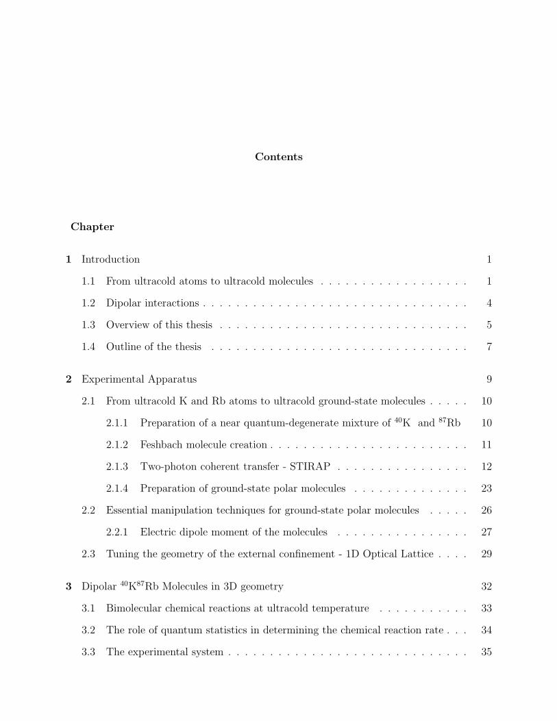
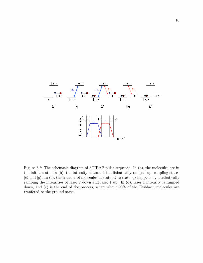
2.2 The schematic diagram of STIRAP pulse sequence. In (a), the molecules are

in the initial state. In (b), the intensity of laser 2 is adiabatically ramped

up, coupling states |e〉 and |g〉. In (c), the transfer of molecules in state |i〉to state |g〉 happens by adiabatically ramping the intensities of laser 2 down

and laser 1 up. In (d), laser 1 intensity is ramped down, and (e) is the end of

the process, where about 90% of the Feshbach molecules are tranfered to the

ground state. . . . . . . . . . . . . . . . . . . . . . . . . . . . . . . . . . . . 16

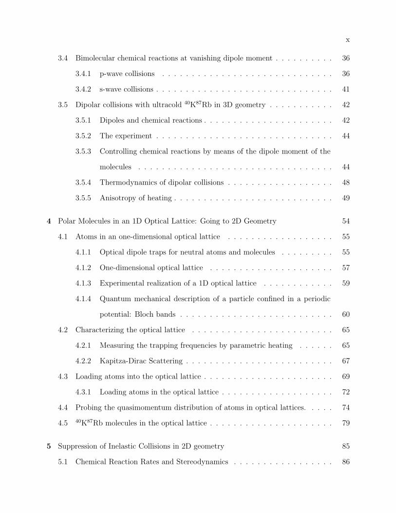
2.3 Schematic picture of the spectrum of the frequency comb. The two CW lasers

at frequencies ν690 and ν970 are phase-locked to the comb. . . . . . . . . . . . 18

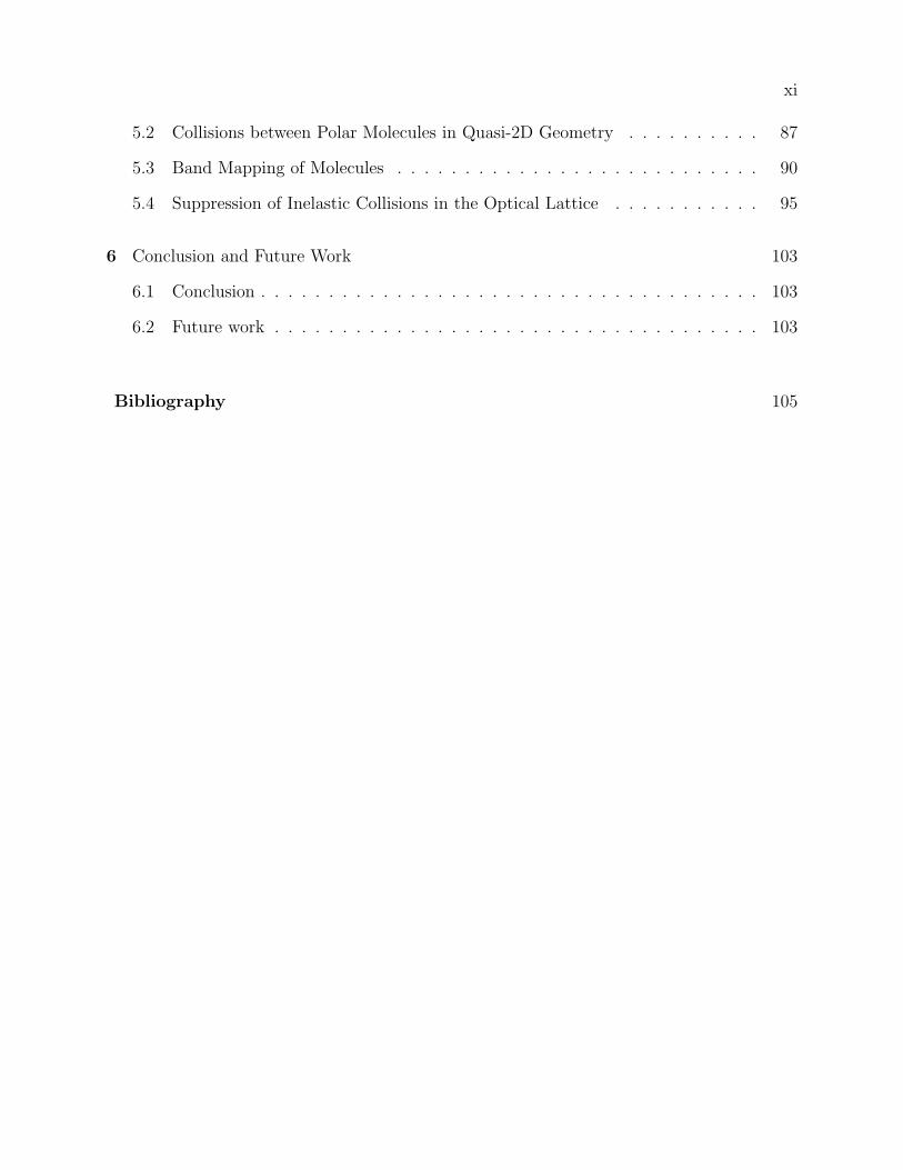
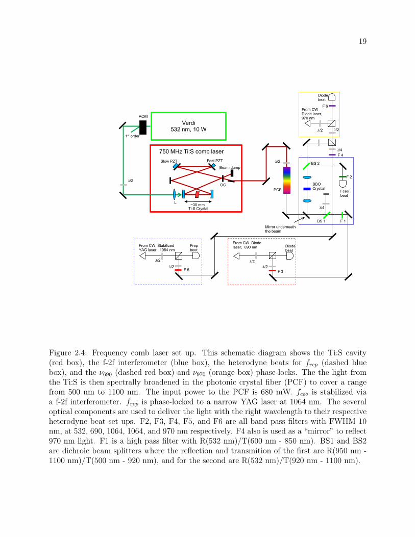
2.4 Frequency comb laser set up. This schematic diagram shows the Ti:S cavity

(red box), the f-2f interferometer (blue box), the heterodyne beats for frep

(dashed blue box), and the ν690 (dashed red box) and ν970 (orange box) phase-

locks. The the light from the Ti:S is then spectrally broadened in the photonic

crystal fiber (PCF) to cover a range from 500 nm to 1100 nm. The input power

to the PCF is 680 mW. fceo is stabilized via a f-2f interferometer. frep is phase-

locked to a narrow YAG laser at 1064 nm. The several optical components

are used to deliver the light with the right wavelength to their respective

heterodyne beat set ups. F2, F3, F4, F5, and F6 are all band pass filters with

FWHM 10 nm, at 532, 690, 1064, 1064, and 970 nm respectively. F4 also is

used as a “mirror” to reflect 970 nm light. F1 is a high pass filter with R(532

nm)/T(600 nm - 850 nm). BS1 and BS2 are dichroic beam splitters where the

reflection and transmition of the first are R(950 nm - 1100 nm)/T(500 nm -

920 nm), and for the second are R(532 nm)/T(920 nm - 1100 nm). . . . . . . 19

xiv

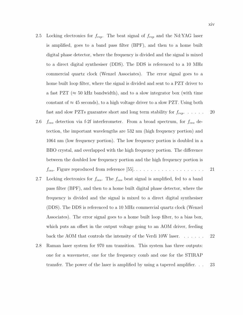
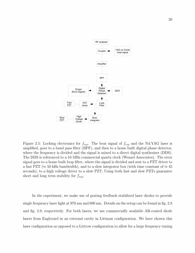
2.5 Locking electronics for frep. The beat signal of frep and the Nd:YAG laser

is amplified, goes to a band pass filter (BPF), and then to a home built

digital phase detector, where the frequency is divided and the signal is mixed

to a direct digital synthesiser (DDS). The DDS is referenced to a 10 MHz

commercial quartz clock (Wenzel Associates). The error signal goes to a

home built loop filter, where the signal is divided and sent to a PZT driver to

a fast PZT (≈ 50 kHz bandwidth), and to a slow integrator box (with time

constant of ≈ 45 seconds), to a high voltage driver to a slow PZT. Using both

fast and slow PZTs guarantee short and long term stability for frep. . . . . . 20

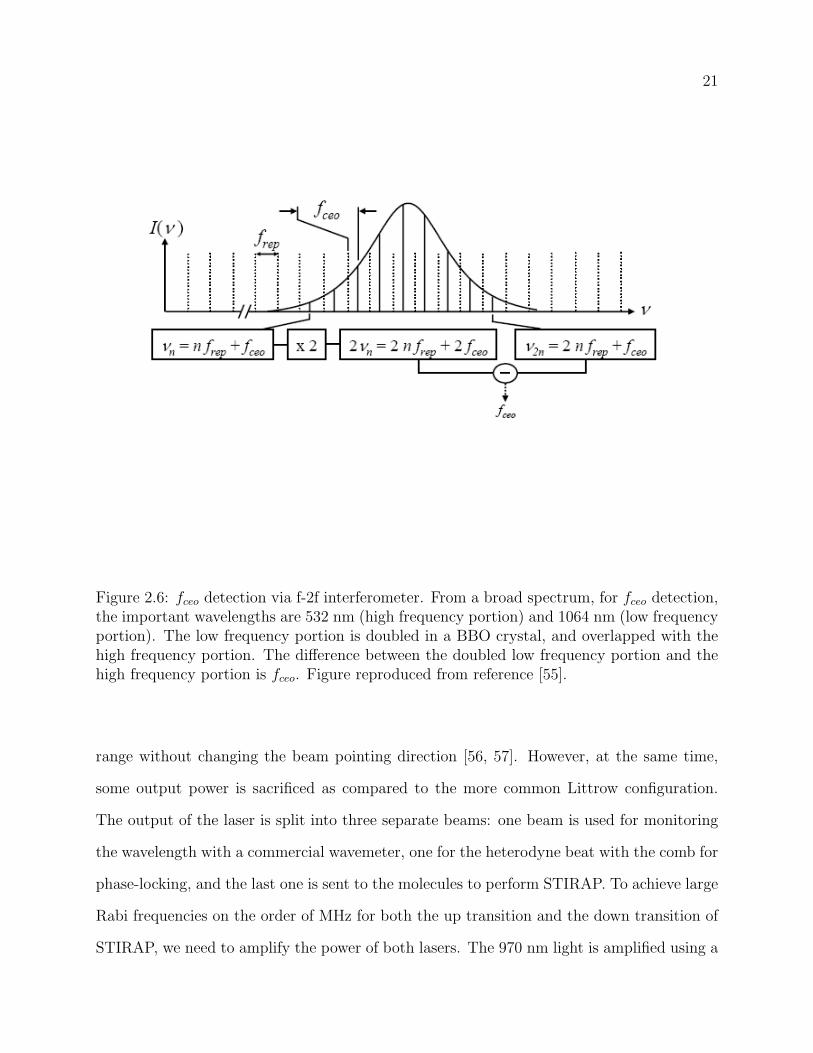
2.6 fceo detection via f-2f interferometer. From a broad spectrum, for fceo de-

tection, the important wavelengths are 532 nm (high frequency portion) and

1064 nm (low frequency portion). The low frequency portion is doubled in a

BBO crystal, and overlapped with the high frequency portion. The difference

between the doubled low frequency portion and the high frequency portion is

fceo. Figure reproduced from reference [55]. . . . . . . . . . . . . . . . . . . . 21

2.7 Locking electronics for fceo. The fceo beat signal is amplified, fed to a band

pass filter (BPF), and then to a home built digital phase detector, where the

frequency is divided and the signal is mixed to a direct digital synthesiser

(DDS). The DDS is referenced to a 10 MHz commercial quartz clock (Wenzel

Associates). The error signal goes to a home built loop filter, to a bias box,

which puts an offset in the output voltage going to an AOM driver, feeding

back the AOM that controls the intensity of the Verdi 10W laser. . . . . . . 22

2.8 Raman laser system for 970 nm transition. This system has three outputs:

one for a wavemeter, one for the frequency comb and one for the STIRAP

transfer. The power of the laser is amplified by using a tapered amplifier. . . 23

xv

2.9 Raman laser system for 690 nm transition. This system has three outputs:

one for a wavemeter, one for the frequency comb and one for the STIRAP

transfer. The power of the laser is amplified by using another diode laser

(slave laser) seeded with ≈ 1 mW of power from the master laser. The slave

laser is locked via injection lock. . . . . . . . . . . . . . . . . . . . . . . . . . 24

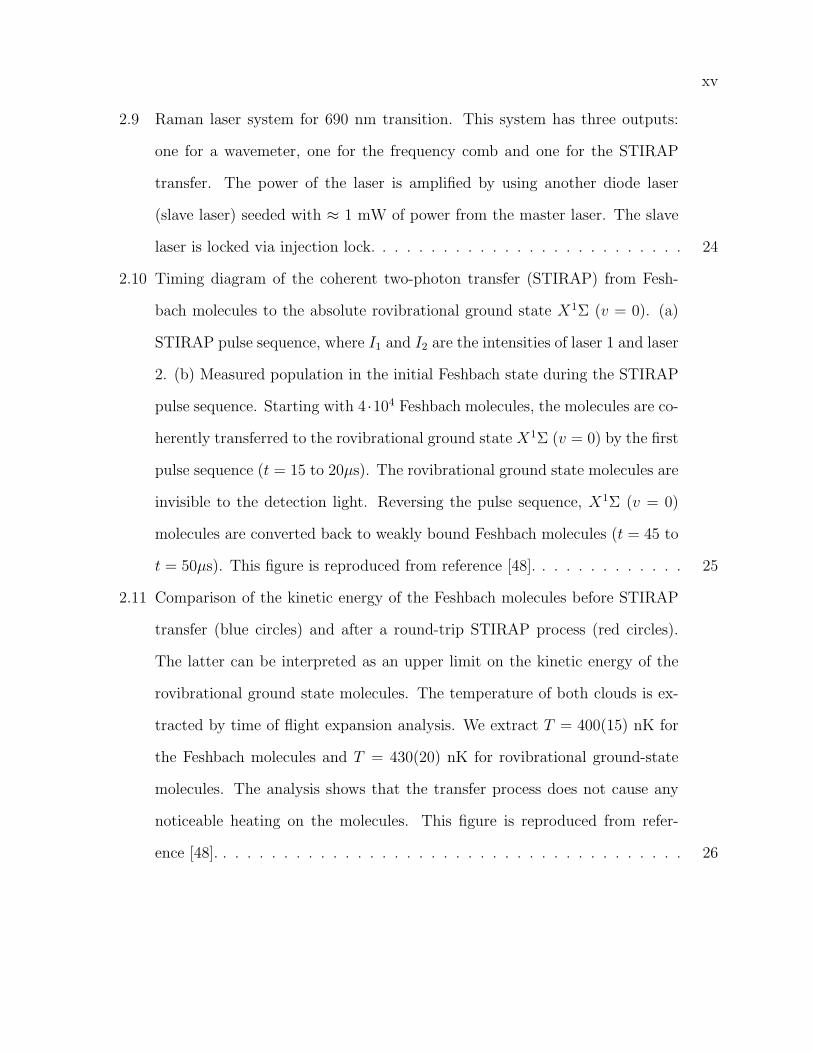
2.10 Timing diagram of the coherent two-photon transfer (STIRAP) from Fesh-

bach molecules to the absolute rovibrational ground state X1Σ (v = 0). (a)

STIRAP pulse sequence, where I1 and I2 are the intensities of laser 1 and laser

2. (b) Measured population in the initial Feshbach state during the STIRAP

pulse sequence. Starting with 4 ·104 Feshbach molecules, the molecules are co-

herently transferred to the rovibrational ground state X1Σ (v = 0) by the first

pulse sequence (t = 15 to 20µs). The rovibrational ground state molecules are

invisible to the detection light. Reversing the pulse sequence, X1Σ (v = 0)

molecules are converted back to weakly bound Feshbach molecules (t = 45 to

t = 50µs). This figure is reproduced from reference [48]. . . . . . . . . . . . . 25

2.11 Comparison of the kinetic energy of the Feshbach molecules before STIRAP

transfer (blue circles) and after a round-trip STIRAP process (red circles).

The latter can be interpreted as an upper limit on the kinetic energy of the

rovibrational ground state molecules. The temperature of both clouds is ex-

tracted by time of flight expansion analysis. We extract T = 400(15) nK for

the Feshbach molecules and T = 430(20) nK for rovibrational ground-state

molecules. The analysis shows that the transfer process does not cause any

noticeable heating on the molecules. This figure is reproduced from refer-

ence [48]. . . . . . . . . . . . . . . . . . . . . . . . . . . . . . . . . . . . . . . 26

xvi

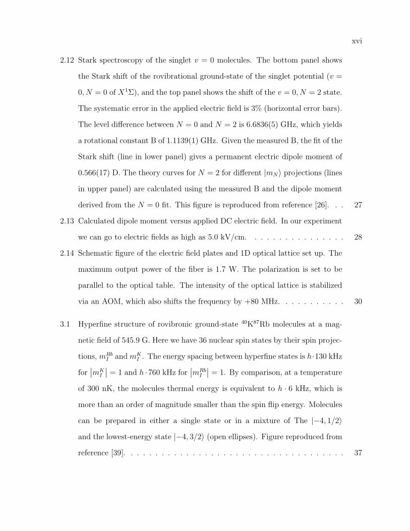
2.12 Stark spectroscopy of the singlet v = 0 molecules. The bottom panel shows

the Stark shift of the rovibrational ground-state of the singlet potential (v =

0, N = 0 of X1Σ), and the top panel shows the shift of the v = 0, N = 2 state.

The systematic error in the applied electric field is 3% (horizontal error bars).

The level difference between N = 0 and N = 2 is 6.6836(5) GHz, which yields

a rotational constant B of 1.1139(1) GHz. Given the measured B, the fit of the

Stark shift (line in lower panel) gives a permanent electric dipole moment of

0.566(17) D. The theory curves for N = 2 for different |mN〉 projections (lines

in upper panel) are calculated using the measured B and the dipole moment

derived from the N = 0 fit. This figure is reproduced from reference [26]. . . 27

2.13 Calculated dipole moment versus applied DC electric field. In our experiment

we can go to electric fields as high as 5.0 kV/cm. . . . . . . . . . . . . . . . 28

2.14 Schematic figure of the electric field plates and 1D optical lattice set up. The

maximum output power of the fiber is 1.7 W. The polarization is set to be

parallel to the optical table. The intensity of the optical lattice is stabilized

via an AOM, which also shifts the frequency by +80 MHz. . . . . . . . . . . 30

3.1 Hyperfine structure of rovibronic ground-state 40K87Rb molecules at a mag-

netic field of 545.9 G. Here we have 36 nuclear spin states by their spin projec-

tions, mRbI and mK

I . The energy spacing between hyperfine states is h·130 kHz

for∣∣mK

I

∣∣ = 1 and h ·760 kHz for∣∣mRb

I

∣∣ = 1. By comparison, at a temperature

of 300 nK, the molecules thermal energy is equivalent to h · 6 kHz, which is

more than an order of magnitude smaller than the spin flip energy. Molecules

can be prepared in either a single state or in a mixture of The |−4, 1/2〉and the lowest-energy state |−4, 3/2〉 (open ellipses). Figure reproduced from

reference [39]. . . . . . . . . . . . . . . . . . . . . . . . . . . . . . . . . . . . 37

xvii

3.2 Transfer from the rovibrational ground state |−4, 1/2〉 to the absolute ground

state |−4, 3/2〉 via coherent Rabi transfer. The intermediate state is in the

rotational level N = 1 and it is a mixed state with g≈ 5 %. . . . . . . . . . . 38

3.3 Inelastic collisions between spin-polarized (indistinguishable) or different spin-

state (distinguishable) fermionic molecules in the rovibronic ground state of

40K87Rb. (A) Data showing the time dependence of the molecule number den-

sity. Here the molecules are prepared in a single hyperfine state, |−4, 1/2〉, and

the molecular density decays slowly with a rate coefficient of 3.3(±0.7) · 1012

cm3 s−1 at T = 250 nK. (B) Loss rate coefficient as function of the temper-

ature. The loss rate increases linearly with temperature for spin-polarized

molecules, which collide via p-wave [inset in (A)] at low temperature. Data

were taken for molecules prepared in either |−4, 1/2〉 (solid circles) or the

lowest-energy state |−4, 3/2〉 (open triangles). A linear fit (solid line) to the

|−4, 1/2〉 data yields the temperature-dependent loss rate to be 1.2(±0.3) ·105

cm3 s−1 K−1. For the |−4, 3/2〉 case, where the collisional loss can only be

due to chemically reactive scattering, the loss rate is similar. The dotted and

dashed lines are the predictions from the QT and MQDT models, respectively.

When the molecules are prepared in a mixture of the |−4, 1/2〉 and |−4, 3/2〉states (solid squares), we observe a temperature-independent decay rate that

is 10 to 100 times that for the spin-polarized case. Figure reproduced from

reference [39]. . . . . . . . . . . . . . . . . . . . . . . . . . . . . . . . . . . . 41

3.4 p-wave barrier for 40K87Rb dipolar collisions “head-to-tail” (solid curve in

blue) and “side-by-side” (solid curve in red). The dashed line represents the

p-wave in the absence of electric-field. . . . . . . . . . . . . . . . . . . . . . . 43

xviii

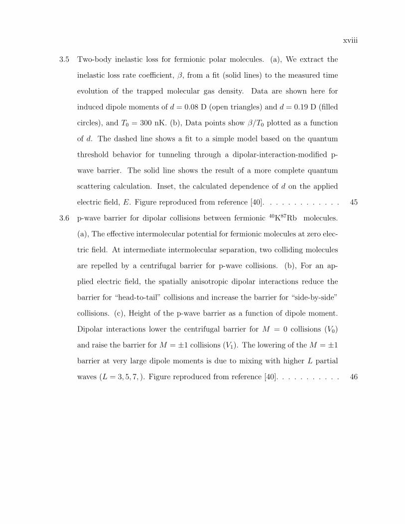
3.5 Two-body inelastic loss for fermionic polar molecules. (a), We extract the

inelastic loss rate coefficient, β, from a fit (solid lines) to the measured time

evolution of the trapped molecular gas density. Data are shown here for

induced dipole moments of d = 0.08 D (open triangles) and d = 0.19 D (filled

circles), and T0 = 300 nK. (b), Data points show β/T0 plotted as a function

of d. The dashed line shows a fit to a simple model based on the quantum

threshold behavior for tunneling through a dipolar-interaction-modified p-

wave barrier. The solid line shows the result of a more complete quantum

scattering calculation. Inset, the calculated dependence of d on the applied

electric field, E. Figure reproduced from reference [40]. . . . . . . . . . . . . 45

3.6 p-wave barrier for dipolar collisions between fermionic 40K87Rb molecules.

(a), The effective intermolecular potential for fermionic molecules at zero elec-

tric field. At intermediate intermolecular separation, two colliding molecules

are repelled by a centrifugal barrier for p-wave collisions. (b), For an ap-

plied electric field, the spatially anisotropic dipolar interactions reduce the

barrier for “head-to-tail” collisions and increase the barrier for “side-by-side”

collisions. (c), Height of the p-wave barrier as a function of dipole moment.

Dipolar interactions lower the centrifugal barrier for M = 0 collisions (V0)

and raise the barrier for M = ±1 collisions (V1). The lowering of the M = ±1

barrier at very large dipole moments is due to mixing with higher L partial

waves (L = 3, 5, 7, ). Figure reproduced from reference [40]. . . . . . . . . . . 46

xix

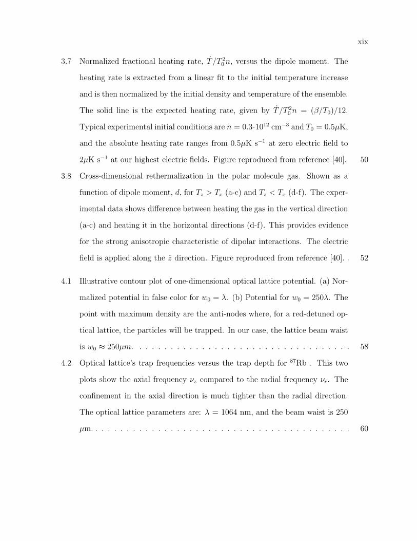
3.7 Normalized fractional heating rate, T /T 20 n, versus the dipole moment. The

heating rate is extracted from a linear fit to the initial temperature increase

and is then normalized by the initial density and temperature of the ensemble.

The solid line is the expected heating rate, given by T /T 20 n = (β/T0)/12.

Typical experimental initial conditions are n = 0.3·1012 cm−3 and T0 = 0.5µK,

and the absolute heating rate ranges from 0.5µK s−1 at zero electric field to

2µK s−1 at our highest electric fields. Figure reproduced from reference [40]. 50

3.8 Cross-dimensional rethermalization in the polar molecule gas. Shown as a

function of dipole moment, d, for Tz > Tx (a-c) and Tz < Tx (d-f). The exper-

imental data shows difference between heating the gas in the vertical direction

(a-c) and heating it in the horizontal directions (d-f). This provides evidence

for the strong anisotropic characteristic of dipolar interactions. The electric

field is applied along the z direction. Figure reproduced from reference [40]. . 52

4.1 Illustrative contour plot of one-dimensional optical lattice potential. (a) Nor-

malized potential in false color for w0 = λ. (b) Potential for w0 = 250λ. The

point with maximum density are the anti-nodes where, for a red-detuned op-

tical lattice, the particles will be trapped. In our case, the lattice beam waist

is w0 ≈ 250µm. . . . . . . . . . . . . . . . . . . . . . . . . . . . . . . . . . . 58

4.2 Optical lattice’s trap frequencies versus the trap depth for 87Rb . This two

plots show the axial frequency νz compared to the radial frequency νr. The

confinement in the axial direction is much tighter than the radial direction.

The optical lattice parameters are: λ = 1064 nm, and the beam waist is 250

µm. . . . . . . . . . . . . . . . . . . . . . . . . . . . . . . . . . . . . . . . . . 60

xx

4.3 Bloch bands in the one-dimensional optical lattice. Energy versus quasimo-

mentum in the first Brillouin zone for different lattice depths. The lattice

depths are 0, 10, 15, and 20 Erec. As the lattice height increases, the sepa-

ration between the Bloch bands also increases and the energy levels flattens

out. . . . . . . . . . . . . . . . . . . . . . . . . . . . . . . . . . . . . . . . . 62

4.4 First four energy levels versus the lattice depth with quasimomentum q = 0,

for an atom in an optical lattice. For lattice depths above 30Erec, the spacing

between the energy levels approaches ~ωz like a harmonic oscillator energy. . 63

4.5 Semi-log plot of tunneling time in an 1D optical lattice versus lattice depth.

Dotted blue line is for 40K and red dashed line is for 87Rb . For our typical

conditions, the tunneling time for 40K is 300 ms (for 19 EKrec) and for 87Rb is

1 s (for 42 ERbrec). . . . . . . . . . . . . . . . . . . . . . . . . . . . . . . . . . 65

4.6 Trap frequency measurement for Feshbach molecules 40K-87Rb via paramet-

ric heating. σ is the molecular cloud width in the z direction. The center

frequency is 44 kHz, which indicates that the axial frequency of the optical

lattice is 22 kHz. The ramp procedure for this measurement is similar to the

one described in chapter 5 in fig. 5.2 except with a sudden turn off of the end

of the ramp. . . . . . . . . . . . . . . . . . . . . . . . . . . . . . . . . . . . . 67

4.7 Ramp procedure to measure trap depth of the optical lattice. The depth

measurement is done with a 87Rb BEC. The optical lattice is diabatically

pulsed on and briefly switched off in order to excite 87Rb atoms to higher

bands. The hold time is varied on the order of tens of microseconds. The

time of flight is 5 ms, and the lattice height is 42 Erec. . . . . . . . . . . . . 69

4.8 87Rb BEC matter-wave diffraction into discrete momentum components. . . 70

xxi

4.9 Extracted relative population of momentum components versus pulse dura-

tion. The lines show a fit to eq. 4.19. The optical lattice depth as a free

parameter, and the extracted one from the data is 42 Erec. The optical lattice

parameters are λ = 1064 nm, beam waist of 250 µm, and laser power of 1

W. The three curves show the 0~k (solid blue), ±2~k (solid green), and ±4~k

(solid red) momentum components. . . . . . . . . . . . . . . . . . . . . . . . 71

4.10 Energy gap between lowest and first excited Bloch bands for different quasi-

momenta. Solid blue line is for q = 0, dashed green line is for q = 0.5 ~k, and

red dotted line is for q = ~k. . . . . . . . . . . . . . . . . . . . . . . . . . . . 72

4.11 Ramping procedure to adiabatically load 40K and 87Rb in the optical lattice.

The optical lattice depth for 87Rb is 42 ERbrec and for 40K is 19 EK

rec. . . . . . 73

4.12 Lifetime of 87Rb and 40K atoms and respective heating rates in the optical

lattice. . . . . . . . . . . . . . . . . . . . . . . . . . . . . . . . . . . . . . . . 74

4.13 Calculated functions for the distribution in quasimomentum space at the first

Brillouin zone in the optical lattice. Red dotted curve is a gaussian function,

green dashed curve is a Heaviside function, and solid blue line is the convolved

curve that is used to fit the atomic cloud along the lattice axis. . . . . . . . . 75

4.14 Band mapping with filtering of 40K in higher bands. The optical lattice is adi-

abatically ramped up exponentially in 150 ms to 17.7 Erec. At the beginning

the optical lattice and the optical trap are combined to hold the atoms against

the gravity. The filtering is done for two different lattice heights: 3.2 Erec,

and 14.5 Erec. . . . . . . . . . . . . . . . . . . . . . . . . . . . . . . . . . . . 76

xxii

4.15 Band mapping for the filtering procedure with 40K atoms. (a), and (c) are the

atomic cloud images taken with time of flight of 18 ms. The initial temperature

of the atoms in (a) is 350 nK and in (b) is 400 nK. The vertical profiles are

shown in (b) and (d). In (b) all atoms are in the first Brillouin zone, while

in (d) about 28% of the atoms are in the second Brillouin zone. However, a

significantly difference in population of bands is observed in the two cases due

to a different optical lattice heights (3.2 Erec, and 14.5 Erec) applied for the

filtering proceedure(see fig. 4.14). . . . . . . . . . . . . . . . . . . . . . . . . 79

4.16 Ramping procedure for formation of ground state 40K87Rb molecules in the

optical lattice. The final lattice depth is 60 EKRbrec . . . . . . . . . . . . . . . . 81

4.17 Heating rate for 40K87Rb in the optical lattice. The optical lattice depth is

60 EKRbrec depth. . . . . . . . . . . . . . . . . . . . . . . . . . . . . . . . . . . 82

4.18 Ramp procedure for forming/loading ground state molecules in the optical

lattice. The number 1 indicates where the ground state molecules are formed.

Then the molecules are loaded in the optical lattice. The number 2 indicates

where the ground state molecules are formed. In this case the molecules

are formed in the fully ramped up optical lattice. The arrow with the note

“Variable Height” means that the final value of the lattice is changed. The

maximum height (depth) value that the lattice can go is 120 EKRbrec . . . . . . 82

4.19 Measurement of the number of ground state molecules versus the optical

lattice depth. The black open circles show the molecule number when the

molecules are formed in the fully ramped-up optical lattice. The red open

squares show the molecule number when the molecules are formed in the par-

tially ramped up optical lattice. . . . . . . . . . . . . . . . . . . . . . . . . . 83

xxiii

4.20 Ramp procedure for forming/loading ground state molecules in the optical

lattice. The number 3 indicates where the ground state molecules are formed.

The molecules are formed in a partially ramped up optical lattice. The arrow

with the note “Variable Height” means that the partial value of the lattice is

changed. The final height (depth) value of the lattice is 120 EKRbrec . . . . . . . 84

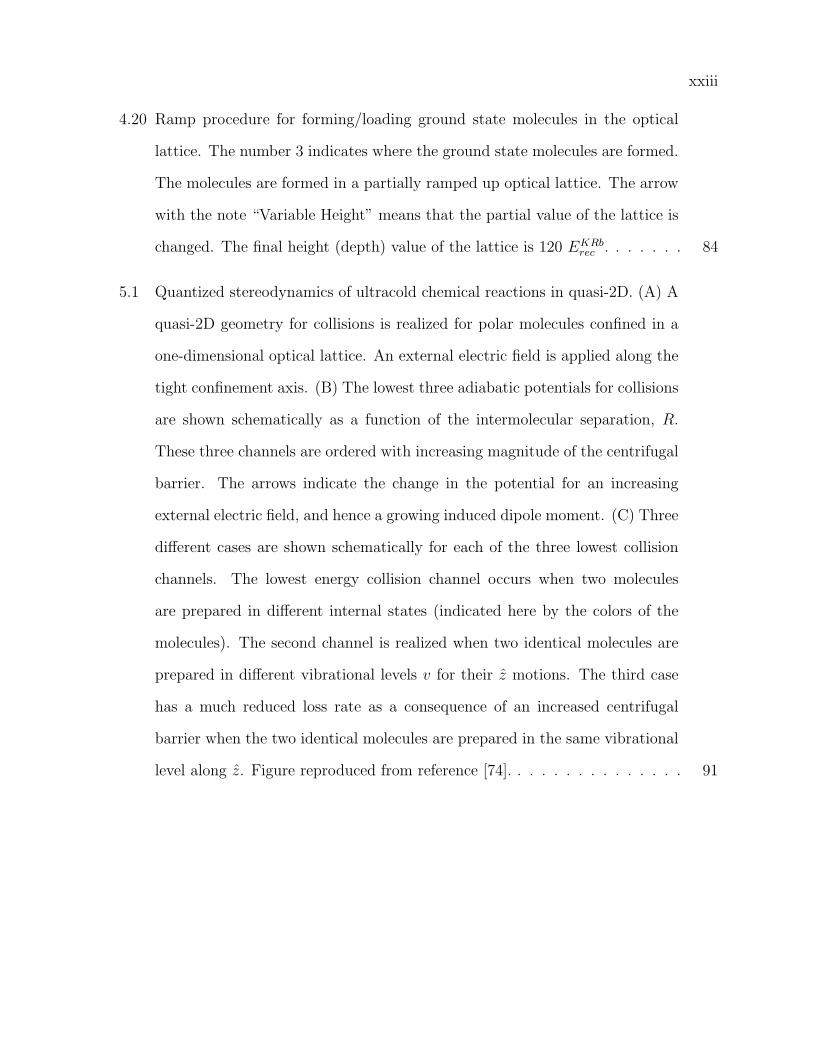
5.1 Quantized stereodynamics of ultracold chemical reactions in quasi-2D. (A) A

quasi-2D geometry for collisions is realized for polar molecules confined in a

one-dimensional optical lattice. An external electric field is applied along the

tight confinement axis. (B) The lowest three adiabatic potentials for collisions

are shown schematically as a function of the intermolecular separation, R.

These three channels are ordered with increasing magnitude of the centrifugal

barrier. The arrows indicate the change in the potential for an increasing

external electric field, and hence a growing induced dipole moment. (C) Three

different cases are shown schematically for each of the three lowest collision

channels. The lowest energy collision channel occurs when two molecules

are prepared in different internal states (indicated here by the colors of the

molecules). The second channel is realized when two identical molecules are

prepared in different vibrational levels v for their z motions. The third case

has a much reduced loss rate as a consequence of an increased centrifugal

barrier when the two identical molecules are prepared in the same vibrational

level along z. Figure reproduced from reference [74]. . . . . . . . . . . . . . . 91

xxiv

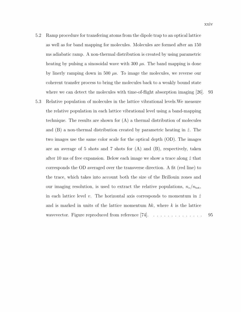
5.2 Ramp procedure for transfering atoms from the dipole trap to an optical lattice

as well as for band mapping for molecules. Molecules are formed after an 150

ms adiabatic ramp. A non-thermal distribution is created by using parametric

heating by pulsing a sinosoidal wave with 300 µs. The band mapping is done

by linerly ramping down in 500 µs. To image the molecules, we reverse our

coherent transfer process to bring the molecules back to a weakly bound state

where we can detect the molecules with time-of-flight absorption imaging [26]. 93

5.3 Relative population of molecules in the lattice vibrational levels.We measure

the relative population in each lattice vibrational level using a band-mapping

technique. The results are shown for (A) a thermal distribution of molecules

and (B) a non-thermal distribution created by parametric heating in z. The

two images use the same color scale for the optical depth (OD). The images

are an average of 5 shots and 7 shots for (A) and (B), respectively, taken

after 10 ms of free expansion. Below each image we show a trace along z that

corresponds the OD averaged over the transverse direction. A fit (red line) to

the trace, which takes into account both the size of the Brillouin zones and

our imaging resolution, is used to extract the relative populations, nv/ntot,

in each lattice level v. The horizontal axis corresponds to momentum in z

and is marked in units of the lattice momentum ~k, where k is the lattice

wavevector. Figure reproduced from reference [74]. . . . . . . . . . . . . . . 95

xxv

5.4 Ramp procedure for measurement of chemical reaction rates. The 40K87Rb molecules

are produced when the optical lattice is fully formed at ≈ 100 Erec, after 150

ms ramp time. The molecules can be excited to higher vibrational levels of

the optical lattice via parametric heating. The parametric heating is done via

a sinosoidal modulation of the lattice intensity for 300 µs. The electric field

is turned on together with the parametric heating and it is turned off 5 ms

before we switch off the dipolar trap and the optical lattice. The molecules

are held in the combined dipolar trap and the optical lattice for a variable

time. After the molecules are released from the trap, the image is taken after

10 ms time of flight. . . . . . . . . . . . . . . . . . . . . . . . . . . . . . . . 97

5.5 Measurements of 2D loss rates and comparison with theory. (A) A fit (solid

lines) to the measured loss curves, with (red circles) and without (black

squares) 0.3 ms of parametric heating in z, is used to extract the loss rate

constants β|3〉 and β|2〉. (B) The extracted loss rate constants for collisions

of molecules in the same lattice vibrational level (black squares) and from

different lattice vibrational levels (red circles) are plotted for several dipole

moments. Measured loss rate constants for molecules prepared in different in-

ternal states are shown as green triangles. For comparison with each of these

three measurements, we include a quantum scattering calculation for νz = 23

kHz, T = 800 nK (solid lines). The potentials corresponding to the dominant

loss channel for the three cases are shown in matching colors in fig. 5.1 B.

Figure reproduced from reference [74]. . . . . . . . . . . . . . . . . . . . . . 101

xxvi

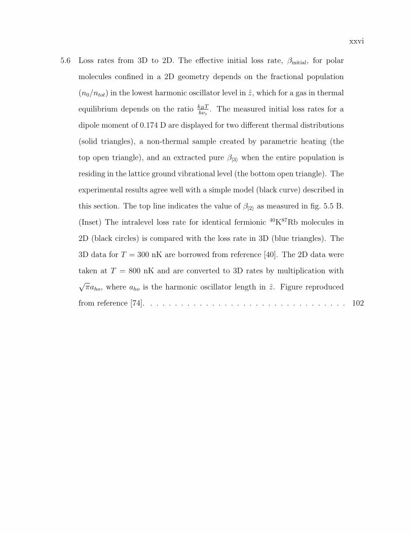
5.6 Loss rates from 3D to 2D. The effective initial loss rate, βinitial, for polar

molecules confined in a 2D geometry depends on the fractional population

(n0/ntot) in the lowest harmonic oscillator level in z, which for a gas in thermal

equilibrium depends on the ratio kBThνz

. The measured initial loss rates for a

dipole moment of 0.174 D are displayed for two different thermal distributions

(solid triangles), a non-thermal sample created by parametric heating (the

top open triangle), and an extracted pure β|3〉 when the entire population is

residing in the lattice ground vibrational level (the bottom open triangle). The

experimental results agree well with a simple model (black curve) described in

this section. The top line indicates the value of β|2〉 as measured in fig. 5.5 B.

(Inset) The intralevel loss rate for identical fermionic 40K87Rb molecules in

2D (black circles) is compared with the loss rate in 3D (blue triangles). The

3D data for T = 300 nK are borrowed from reference [40]. The 2D data were

taken at T = 800 nK and are converted to 3D rates by multiplication with

√πaho, where aho is the harmonic oscillator length in z. Figure reproduced

from reference [74]. . . . . . . . . . . . . . . . . . . . . . . . . . . . . . . . . 102

Chapter 1

Introduction

1.1 From ultracold atoms to ultracold molecules

Over the last decades, the field of ultracold atoms has progressed at a tremendous pace.

Initial experiments focused on the development of techniques to cool and trap atoms [1, 2, 3],

including the decisive techniques of laser cooling and evaporative cooling. Based on these

techniques very exciting and important milestones have been achieved: The preparation of

Bose-Einstein condensates (BEC) [4, 5, 6, 7] and quantum degenerate Fermi gases in dilute

atomic gases [8] opened new avenues in atomic physics. Fano-Feshbach resonances allowed

control of atom-atom interactions [9]. This created novel opportunities such as the realization

of strongly interacting systems, the study of BEC-BCS crossover physics [10, 11, 12], and the

preparation of ultracold weakly bound Feshbach molecules [13, 14] from quantum degenerate

gases of atoms.

Compared to atomic quantum systems, molecular quantum systems promise to open

new research frontiers. However, the molecules’ complex internal structure makes molecular

systems very rich but also really challenging. Due to numerous vibrational and rotational

quantum degrees of freedom, traditional cooling methods for atoms have not worked for

molecules. Experimental efforts towards the creation of quantum gases of molecules have

therefore followed two distinct paths. The first approach is to directly cool molecules to

low translational temperatures. This can be achieved by Stark deceleration or buffer gas

cooling [15, 16, 17]. Unfortunately, these techniques have so far been limited to low densities

2

(108 molecules/cm3) and relatively high temperatures in the miliKelvin range. These param-

eters correspond to a phase-space density of 10−13 and therefore many orders of magnitude

away from quantum degeneracy. The second way is to cool and trap atoms first and then

associate pairs of cold atoms to tightly bound molecules. A challenge here is the efficient

conversion of free atoms to molecules while preserving density and temperature of the initial

atomic ensemble. In 2005, Sage et al. [18], demonstrated the formation of vibrational ground

state RbCs molecules formed via photoassociation from free atoms. Starting from a laser

cooled atomic ensemble of 2 × 108 Rb and 3 × 108 Cs atoms at temperatures of 100 µK

and phase space densities on the order of 10−14, they obtained a conversion efficiency of

few percent [18]. These experiments elucidated that to achieve better conversion efficien-

cies and higher phase space densities, the initial conditions of the atomic ensemble needs to

be far closer to quantum degeneracy and the conversion process from free atoms to deeply

bound molecules needs to be very efficient. In our lab, this was achieved by combining two

techniques. The first is Feshbach molecule creation in ultracold quantum degenerate atomic

gases, which allows the efficient conversion of atomic ensembles into weakly bound molecules

prepared in a well-defined quantum state.

The next challenge was to transfer the weakly bound molecules into their absolute

ground state. Our goal is to transfer to a single internal quantum state without heating the

sample of molecules. Therefore, a fully coherent conversion process was needed. The conver-

sion efficiency is also essential to preserve the initial high phase-space density. A technique

known as STImulated Raman Adiabatic Passage (STIRAP) [19], involving an electronically

excited intermediate state, can be envisioned for the transfer process between the initial

and final vibration levels. Because of a nearly complete mismatch between the vibrational

wave-functions of the weakly bound and the absolute ground-state molecules, it was largely

believed to be impossible to find a suitable intermediate state that could provide sufficient

transition strengths for both the upward and downward transitions. A proposal was made

to use a train of two-color, phase-coherent pulses that would allow coherent accumulations

3

of a pump-dump process to implement a fully coherent molecular conversion process [20].

However, systematic and detailed single photon spectroscopy ensued [21], connecting the ini-

tial Feshbach state to specific electronically excited states with a CW laser referenced to an

optical frequency comb. An intense theory-experiment collaboration led us to the realization

that we could use a single stationary intermediate state instead of dynamic wave-packets,

which a key point is to have an intermediate state that provides favorable Franck-Condon

factors to both the initial weakly bound Feshbach state and the rovibrational ground state.

Coherent conversion of weakly bound molecules into a more deeply bound states has

been demonstrated in several experiments [22]. In the work done by our group, Ospelkaus

et al. [23], STIRAP is used to convert an ensemble of weakly bound 40K-87Rb molecules,

with binding energy of a few hundred kilohertz, into an ensemble of molecules in a vibra-

tional state bound by more than 10 GHz1 . In 2008, we demonstrated that a single step

of a coherent transfer can even be used to convert an ensemble of heteronuclear Feshbach

molecules into an ensemble of rovibrational ground state polar molecules [26]. In these ex-

periments, the energy difference between the initial and final states is about 125 THz and

therefore it is necessary to establish a fixed phase relation between lasers of extremely dif-

ferent frequencies. This task was accomplished by referencing the two lasers to individual

teeth of an optical frequency comb laser [27, 28, 29]. Using this technique, we demonstrated

the creation of an ultracold high phase space density molecular gas prepared in its lowest

internal quantum state. The resulting ground state molecular ensemble has a peak density

of 1012 molecules/cm3, a temperature of 200 nK, and a phase-space density of 0.06, and is

therefore prepared close to quantum degeneracy. Also, the molecules have an electric dipole

momentum of 0.566 Debye. This opens exciting perspectives for the study of quantum gases

with strong dipole-dipole interaction.

1 Related work has been done for homonuclear molecules of Cs2 and Rb2 by Danzel et al. [24] and Langet al. [25] respectively.

4

1.2 Dipolar interactions

Interactions between particles determines many of the observed phenomena in ultracold

quantum degenerate atomic gases. Interactions profoundly modify the static and also the

dynamic properties of the system [30]. Short-range and isotropic “contact” interactions

dominate the properties of most quantum gases of ultracold atoms, whereas dipole-dipole

interactions play only a negligible role. However, recent developments in the manipulation

of cold atoms and molecules have opened the way for the study of dipole-dipole interparticle

interactions in ultracold quantum gases.

Dipole-dipole interactions have interesting properties. First, the dipole-dipole inter-

action is spatially anisotropic, which means that the strength and sign of the interaction

depends on the relative orientation of the dipoles. Second, the dipole-dipole interaction is

long range, where the interaction decays with 1/r3, r being the interparticle distance. Third,

the electric-dipole moment of molecules is tunable by means of an externally applied field.

Pioneering work on the study of magnetic dipole-dipole interactions in ultracold quan-

tum gases was done in Tilman Pfau’s group [31, 32]. Pfau and coworkers managed to prepare

a Bose-Einstein condensate (BEC) of 52Cr atoms. Chromium has a large magnetic dipole

moment of 6 Bohr magnetons - a factor of 6 larger than the magnetic-dipole moment of

alkali atoms. By enhancing the dipole-dipole interaction by the choice of the atomic species

and making use of Fano-Feshbach resonances in chromium to reduce the isotropic contact

interaction, the group was able to achieve a regime where the anisotropic magnetic dipole-

dipole interaction between 52Cr in the BEC dominates over the short-range interaction. This

allowed the study of the anisotropic character of the dipole-dipole interaction in collision and

expansion dynamics of the atomic gas [32].

However, interactions between magnetic dipole moments of atoms are typically weaker

than those between electric dipole moments of polar molecules. For example, the elec-

tric dipole moment of a typical polar molecule is on the order of 1 Debye, where 1 Debye

5

is ≈ 3.34·10−30 C·m. The interaction energy between polar molecules is then typically a

factor of 10000 times larger than the interaction energy between atoms interacting via mag-

netic dipole-dipole interactions with a typical dipole moment of 1 Bohr magneton (µB),

(1 Debye)2c2

(1 µB)2≈ 104.

Building on the preparation of an ultracold polar gas of fermionic 40K-87Rb molecules

in our group in 2008 [26], a variety of novel experimental possibilities have opened up based

on the control and use of the dipole-dipole interaction between polar molecules. Theoret-

ical proposals range from the study of quantum phase transitions [33] and quantum gas

dynamics [34] to quantum simulations of condensed matter spin systems [35] and schemes

for quantum information processing [36, 37, 38].

1.3 Overview of this thesis

The main work of this thesis is about the confinement of an ensemble of ground-state

polar 40K87Rb molecules in a quasi-2D geometry to control chemical reactions at ultralow

temperature. As a background for my thesis work, I review previous work in ultracold

chemistry of 40K87Rb [39] and dipolar interactions in 3D [40]. These subjects are also dis-

cussed in Kang-Kuen Ni Ph.D. thesis [21] to which I contribute. The chemical reaction

KRb+KRb→K2+Rb2 is exothermic and proceeds without a chemical reaction barrier at

short-range. Starting from fermionic polar molecules close to quantum degeneracy, we study

this atom-exchange chemical reaction in a regime where the motion of the molecules is strictly

quantized. When the ensemble of 40K87Rb molecules is created in a single quantum state

- that means the molecules are indistinguishable fermions - we observe chemical reactions

to be strongly suppressed by a long-range p-wave barrier of 24 µK that effectively hinders

the molecules from coming into short-range [39]. However, changing the quantum statistics

of the molecular ensemble by preparing a 50:50 mixture of two spin states, we observe the

collisional rate to be enhanced by a factor of 10-100. For these distinguishable molecules,

collisions will proceed via the s-wave channel, which means that there is no repulsive colli-

6

sional barrier at long-range. The two molecules easily get within short-range where reaction

loss proceeds with almost unity probability.

With this basic understanding of how chemical reactions occur in the quantum regime,

we make use of the large tunable electric dipole moment to control the long-range potential

between two colliding molecules and therefore the chemical reaction rate. Applying an

external electric field induces a dipole moment in the molecule. The dipole-dipole interaction

will then strongly determine the collisional processes occurring in the sample. Of particular

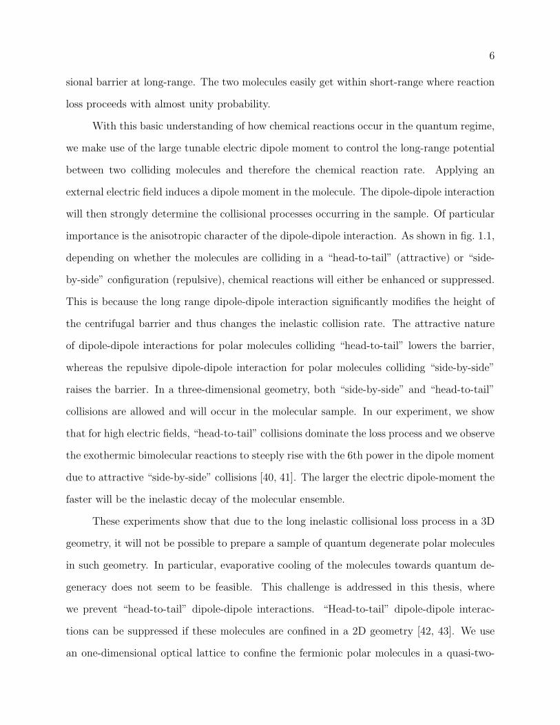
importance is the anisotropic character of the dipole-dipole interaction. As shown in fig. 1.1,

depending on whether the molecules are colliding in a “head-to-tail” (attractive) or “side-

by-side” configuration (repulsive), chemical reactions will either be enhanced or suppressed.

This is because the long range dipole-dipole interaction significantly modifies the height of

the centrifugal barrier and thus changes the inelastic collision rate. The attractive nature

of dipole-dipole interactions for polar molecules colliding “head-to-tail” lowers the barrier,

whereas the repulsive dipole-dipole interaction for polar molecules colliding “side-by-side”

raises the barrier. In a three-dimensional geometry, both “side-by-side” and “head-to-tail”

collisions are allowed and will occur in the molecular sample. In our experiment, we show

that for high electric fields, “head-to-tail” collisions dominate the loss process and we observe

the exothermic bimolecular reactions to steeply rise with the 6th power in the dipole moment

due to attractive “side-by-side” collisions [40, 41]. The larger the electric dipole-moment the

faster will be the inelastic decay of the molecular ensemble.

These experiments show that due to the long inelastic collisional loss process in a 3D

geometry, it will not be possible to prepare a sample of quantum degenerate polar molecules

in such geometry. In particular, evaporative cooling of the molecules towards quantum de-

generacy does not seem to be feasible. This challenge is addressed in this thesis, where

we prevent “head-to-tail” dipole-dipole interactions. “Head-to-tail” dipole-dipole interac-

tions can be suppressed if these molecules are confined in a 2D geometry [42, 43]. We use

an one-dimensional optical lattice to confine the fermionic polar molecules in a quasi-two-

7

dimensional, pancake-like geometry. The dipoles are oriented along the tight axis of con-

finement. The combination of tight confinement (restricting the movement of the molecules

along the axis of strong confinement to a single motional state) and Fermi statistics of the

molecules strictly forbids molecules to approach in a “head-to-tail” configuration. Two po-

lar molecules can approach each other only in a “side-by-side” collision, where the chemical

reaction rate is suppressed by the repulsive dipole-dipole interaction. This quantum stereo-

dynamics of the ultracold collisions can be exploited to suppress the chemical reaction rate by

nearly two orders of magnitude. The suppression of chemical reactions for polar molecules in

a quasi-two-dimensional trap opens the way for investigation of a dipolar molecular quantum

gas.

1.4 Outline of the thesis

Chapter 2 gives a short overview of the experimental set up: the apparatus for the

preparation of a two-species quantum degenerate ensemble of 40K and 87Rb , the creation

of Feshbach molecules, and the laser system for the realization of the STIRAP transfer.

Also, I will review how to realize a two-dimensional geometry by means of a one-dimensional

optical lattice. In Chapter 3, I will discuss basic properties of the dipole-dipole interactions

in 3D geometry, which sets the stage for 40K87Rb molecules in 2D geometry. In Chapter 4, I

present the basic concepts of a 1D optical lattices, adiabatic loading of 40K and 87Rb atoms

into the lattice, and formation of 40K87Rb molecules in the optical lattice. In Chapter 5, I

discuss and present the suppression of inelastic collisions in the tight confinement regime. In

Chapter 6, I summarize the thesis and discuss future work.

8

Figure 1.1: p-wave centrifugal barrier for dipolar collisions between fermionic polar molecules.(A), The effective intermolecular potential for fermionic molecules at zero electric field.At intermediate intermolecular separation, two colliding molecules are repelled by a largecentrifugal barrier for p-wave collisions. (B), For a relatively small applied electric field, thespatially anisotropic dipolar interactions reduce the barrier for head-to-tail collisions andincrease the barrier for side-by-side collisions. From [40].

Chapter 2

Experimental Apparatus

The basis for the experiments presented in this thesis is a reliable apparatus for the

preparation of high-phase space density gases of ultracold polar 40K-87Rb molecules in their

rotational and vibrational ground state. In this chapter, I will give an overview of the

experimental techniques and the experimental apparatus for the preparation of ground state

polar molecules. As already mentioned in the introduction, our approach for the preparation

of a high-density gas of ultracold ground state polar molecules is to cool and trap the

constituent atoms 40K and 87Rb first and then implement a controlled chemical reaction

at ultracold temperature. The latter is done via a two-step process, where in the first step,

weakly bound molecules with a binding energy of h·300 kHz are formed in the vicinity of a

Fano-Feshbach resonance [44]. These molecules are also called Feshbach molecules (FBM).

Once these FBMs are formed, we transfer the molecules to the electronic, vibrational and

rotational ground state via a single step of STImulated Raman Adiabatic Passage (STIRAP).

In the following, we will call the resulting molecules ground state molecules (GSM). The

heteronuclear 40K87Rb GSMs have an electric-dipole moment of 0.56 Debye [26], which

allows the study of dipolar collisions controlled by external electric fields.

In the following, I will review our experimental path from the preparation of ultracold

40K and 87Rb atoms to the manipulation of ground state molecules. I will also discuss basic

manipulation techniques for the ground-state molecules such as precise control over the dipole

moment of the molecules by means of external electric fields and techniques for controlling

10

the confinement geometry of the molecules via dipole and optical lattice potentials.

2.1 From ultracold K and Rb atoms to ultracold ground-state molecules

2.1.1 Preparation of a near quantum-degenerate mixture of 40K and 87Rb

The starting point for the formation of a high-phase space density gas of ground state

molecules is the preparation of a near quantum-degenerate mixture of two atomic species.

In our case, we are working with the alkali atoms 40K and 87Rb . Both atoms are nowadays

workhorses for atomic physics experiments in the quantum degenerate regime, and cooling

and trapping techniques are therefore well established. In the following, I will briefly sum-

marize the main experimental steps. For more details please refer to the Ph.D. thesis of Josh

Zirbel [45].

Cooling and trapping of 40K and 87Rb starts with a two-species magneto-optical

trap (MOT). Typical atom numbers in the MOTs are 2 − 4 × 109 for Rb and 107 for 40K

, respectively. After a short sub-Doppler cooling, optical pumping and compression state,

these atoms are loaded into a quadrupole magnetic trap, which is then subsequently moved

to a second part of the vacuum apparatus - the so-called science chamber. In the science

chamber, the atoms are transfered into a Ioffe-Pritchard (IP) magnetic trap, where both

87Rb and 40K are cooled to temperatures on the order of 1 µK. This is performed by

evaporative cooling of Rb atoms via microwave radiation, which drives high energy 87Rb

atoms in the stretched |F = 2,mF = 2〉 hyperfine state to an untrapped state |1, 1〉. Here

F is the total atomic spin number and mF is the projection. 40K atoms prepared in the

stretched |9/2, 9/2〉 state are sympathetically cooled in the bath of 87Rb atoms. At the end

of the evaporation in the IP trap, we typically achieve atom numbers of 6− 7× 105 for 40K

and 2− 3× 106 for 87Rb , respectively, at temperature of 1 µK.

Magnetic trapping is restricted to low-field seeking atomic states. However, for the

preparation of Feshbach molecules, often high-field seeking states are needed to access a

11

Fano-Feshbach scattering resonance. Also, it is desirable to be able to choose the magnetic

field freely, independent of any trapping potentials. In a next step, we therefore transfer the

atomic mixture into an optical trap (OT). In our case, the OT is realized using a crossed

beam configuration. In the experiment, we have chosen two elliptically shaped Gaussian

beams with beam waists of 40 µm in the vertical and 200 µm in the horizontal direction,

respectively. These two beams intersect at the center of the IP trap and have a wavelength

of 1064 nm. The potential is pancake-shaped with an aspect ratio of 1:5.

The OT is loaded with 40K and 87Rb in the |9/2, 9/2〉 and |2, 2〉 states, respectively. We

then transfer these atoms to their lowest hyperfine states, |9/2,−9/2〉 and |1, 1〉 performed

via two adiabatic rapid passages, by sweeping RF (for 40K ) and microwave frequencies (for

87Rb ) at a magnetic field of 31.29 G. Choosing these two atomic quantum states has two

distinct advantages. First of all, these quantum states are collisionally stable. Second, they

allow access to a relatively broad Feshbach resonance between 40K and 87Rb at about 546

G [46, 47]. In preparation for Feshbach molecule creation, the magnetic field is ramped to

553.3 G and the atoms are evaporatively cooled closer to quantum degeneracy by decreasing

the depth of the optical trapping potential. This procedure achieves temperatures of 200−300

nK, with 40K and 87Rb numbers of 2.5× 105 and 3.5× 105 - an ideal starting point for the

preparation of 40K87Rb Feshbach molecules.

2.1.2 Feshbach molecule creation

For Feshbach molecule creation, we use a Fano-Feshbach resonance at a magnetic field

of 546.7 G [46, 47]. This Feshbach resonance has a width of approximately 3 G and occurs

via an avoided crossing between the open scattering channel K |F = 9/2,mF = −9/2〉 +

Rb |1, 1〉 and the closed molecular scattering channel K |7/2,−7/2〉 + Rb |1, 0〉. Starting

from a mixture of approximately 2.5 · 105 40K atoms and 3.5 · 105 87Rb atoms at 200 nK

prepared in the optical dipole trap at a magnetic field of 553 G, we ramp the magnetic field

through the Feshbach resonance to a field of 545.90 G in 4 ms. This results in the formation

12

of approximately 6 · 104 Feshbach molecules with an expansion energy of kB · 300nK. At the

magnetic field of 545.9 G, the Feshbach molecules are very weakly bound with a binding

energy of h× 240 kHz and a size of approximately 300 Bohr radii.

In the experiment, we observe conversion efficiencies from free atoms to Feshbach

molecules of about 15 − 25%. The conversion efficiency is somewhat limited by a trade-off

between high phase-space density of the initial atomic gases and good spatial overlap between

the two species. To achieve good spatial overlap, the different quantum statistical character

of 40K (fermion) and 87Rb (bosons) requires a temperature of the atomic gases just at the

onset of quantum degeneracy - instead of starting deep in the quantum degenerate regime.

Another limiting factor for the conversion efficiency is strong inelastic losses between 87Rb

and 40K87Rb in the vicinity of the Feshbach resonance.

2.1.3 Two-photon coherent transfer - STIRAP

To prepare a high phase-space density ensemble of ground-state polar molecules, the

ensemble of Feshbach molecules has to be transfered into the rotational and vibrational

ground-state. The transfer has to be done coherently to preserve density and temperature -

and therefore phase-space density - of the initial Feshbach molecule gas.

We make use of a two-photon coherent transfer to transfer Feshbach molecules, pre-

pared in the least bound vibrational state of the electronic ground-state molecular potential,

to the rotational and vibrational ground state. The rotational and vibrational ground state

is bound by approximately h · 125 THz. A sketch of the scheme is shown in fig. 2.1. The

Feshbach molecule state (|i〉) is coupled via a laser field to a vibrational state in an elec-

tronically excited molecular potential (|e〉). This electronically excited state is then coupled

via a second laser field to the rotational and vibrational ground state (|g〉). Together, the

two laser fields provide an effective coupling between the Feshbach state and the rotational

and vibrational ground state. As the transfer scheme is fully coherent, the weakly bound

Feshbach molecules are directly driven to the rovibrational ground state. This avoids any

13

heating of the molecules due to spontaneously emitted photons.

In the experiment, we make use of a very robust two-photon coherent transfer scheme

- called STIRAP (STImulated Raman adiabatic passage). This specific scheme results in a

robust transfer of the initial quantum state |i〉 to the final quantum state |e〉 without ever

acquiring population in the lossy electronically excited state |e〉. The latter just provides a

bridge between the initial and the final state [19]. Fig. 2.2 shows the details of the specific

pulse sequence for the STIRAP transfer. The experiment starts with the entire molecular

ensemble prepared in the initial state |i〉. Then, via the intensity ramp sequence shown in

fig. 2.2, a coherent superposition is established between the intermediate state |e〉 and the

final state |g〉 with laser 2 field. The intensity of laser 2 is adiabatically ramped down in

5 µs, and at the same time, the intensity of laser is ramped up, performing transfer to the

final state |g〉, without populating |e〉.However, the actual implementation of the single-step of coherent two-photon transfer

is challenging. First, it is very critical to achieve good coupling between the initial Feshbach

state and the final ground molecular state. But these two wavefunctions are vastly different

in size and the direct wavefunction overlap is very small. It is therefore necessary to identify

a bridge in the electronically excited state to achieve the best possible coupling between the

initial and the final state. In short, we need to choose an intermediate state with sufficient

wave function overlap for both initial and final states, i.e. Franck-Condon factor (FCF).

Second, it is critical to have phase coherence between the two lasers involved in the transfer

scheme. This is challenging, because the two lasers bridge a frequency gap of 125 THz and

have therefore vastly different wavelengths. In the following, we will discuss how we address

and solve these experimental challenges.

2.1.3.1 The choice of the intermediate state

As pointed out in the previous paragraph, an appropriate choice of the electronically

excited intermediate molecular state is critical for the preparation of a high-phase density gas

14

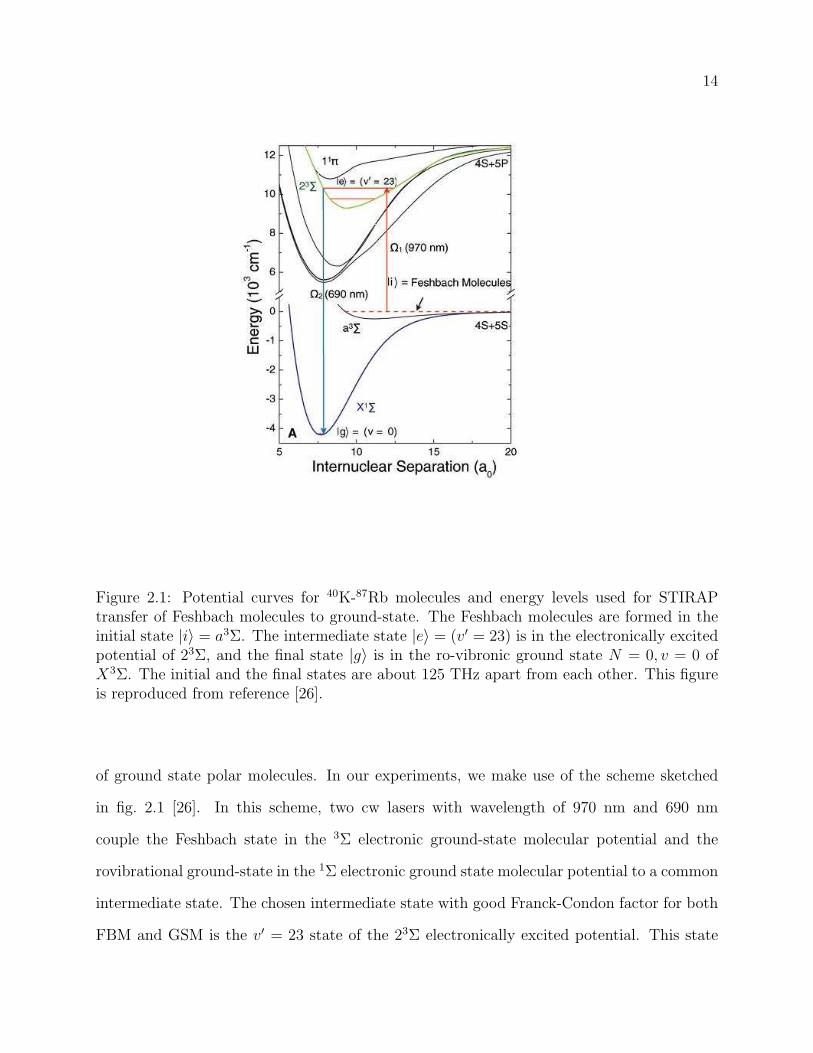
Figure 2.1: Potential curves for 40K-87Rb molecules and energy levels used for STIRAPtransfer of Feshbach molecules to ground-state. The Feshbach molecules are formed in theinitial state |i〉 = a3Σ. The intermediate state |e〉 = (v′ = 23) is in the electronically excitedpotential of 23Σ, and the final state |g〉 is in the ro-vibronic ground state N = 0, v = 0 ofX3Σ. The initial and the final states are about 125 THz apart from each other. This figureis reproduced from reference [26].

of ground state polar molecules. In our experiments, we make use of the scheme sketched

in fig. 2.1 [26]. In this scheme, two cw lasers with wavelength of 970 nm and 690 nm

couple the Feshbach state in the 3Σ electronic ground-state molecular potential and the

rovibrational ground-state in the 1Σ electronic ground state molecular potential to a common

intermediate state. The chosen intermediate state with good Franck-Condon factor for both

FBM and GSM is the v′ = 23 state of the 23Σ electronically excited potential. This state

15

has a small admixture of singlet spin character due to the proximity of the 1Π molecular

potential, which allows the transfer of triplet spin character Feshbach molecules to singlet

spin character rovibrational ground state molecules. The upward transition strength from

the Feshbach molecule state to this intermediate state was determined to be 0.005(2) ea0 [48].

The downward transition strength from the intermediate state to the rovibrational ground

state has been determined to be 0.012(3) ea0 [48].

2.1.3.2 Phase and frequency stabilization of the coherent transfer lasers

In order to implement an efficient coherent transfer between two quantum states using

STIRAP, it is essential to realize good phase coherence between the lasers involved in the

transfer scheme. Loosely speaking, this means that the relative frequency jitter between the

two lasers has to be as small as possible during the time window of the coherent transfer.

In our specific application, achieving good phase coherence is a challenging task, since the

two lasers involved in the transfer scheme are operating at vastly different wavelengths,

corresponding to a frequency difference of 125 THz. A stable two-photon beat between

these two lasers can be maintained by referencing each laser individually to a stable optical

frequency comb.

The frequency comb

Frequency combs are powerful tools for several applications [49, 50, 51, 52, 53]. In our

case, it is used as a stable “frequency ruler”, as shown in fig. 2.3, with 300 THz of spectral

range (from 500 nm to 1100 nm). This frequency ruler is used to phase-lock two Raman

lasers with a frequency difference of 125 THz [26].

The frequency comb used in our experiments is a solid state, ultracompact femtosecond

titanium-sapphire (Ti:S) laser, pumped by a 532 nm Verdi 10W laser from Coherent. The

pump power is 4.9 W (where the maximum power pumped to the Ti:S crystal should be

no higher than 5.5 W). The laser has a ring cavity, with a 750 MHz repetition rate. The

spectrum is centered at 800 nm and is 30 nm wide. The laser was modified to be actively

16

�� � � � ��� �

� �� � �� �� � � � ����� � � � ��� � �� � � � ��� � �� � � � ��� � �� � � � ��� �

��� ��� ��� ��� ������ ��� ��� ��� ���

Figure 2.2: The schematic diagram of STIRAP pulse sequence. In (a), the molecules are inthe initial state. In (b), the intensity of laser 2 is adiabatically ramped up, coupling states|e〉 and |g〉. In (c), the transfer of molecules in state |i〉 to state |g〉 happens by adiabaticallyramping the intensities of laser 2 down and laser 1 up. In (d), laser 1 intensity is rampeddown, and (e) is the end of the process, where about 90% of the Feshbach molecules aretranfered to the ground state.

17

stabilized by controlling two degrees of freedom that determine the frequency of each comb

tooth: the repetition rate, frep, and the carrier-envelope-offset frequency, fceo. The frequency

for each comb tooth is given by the equation:

νn = nfrep ± fceo, (2.1)

where n is a integer number that represents the number of the comb tooth. frep = 750 MHz,

and fceo is in the range of 0 ≤ fceo ≤ frep/2. To be useful as a “frequency ruler”, both frep

and fceo have to be stabilized. In the following, I will detail the stabilization of these two

degrees of freedom.

Frequency comb stabilization

As already mentioned above, the frequency of the teeth of the optical frequency comb

are determined by two degrees of freedom: frep, and fceo. These two degrees of freedom need

to be controlled precisely. The stabilization of frep is realized by controlling the Ti:S laser

cavity length via two piezoelectrics (PZTs) used as actuators. Using these knobs, frep is then

stabilized by referencing a certain frequency tooth in the spectrum of the comb to a stable

1064 nm Nd:YAG. The Nd:YAG laser itself is locked to a stable cavity in John Hall’s lab and

has a linewidth lower than 1 kHz. The locking electronics of frep are shown in fig. 2.5, where

the error signal is fed back to the phase-lock loop electronics to the slow and fast PZTs.

The stabilization of fceo is a bit trickier. It requires a full octave spanning spectrum.

To expand the Ti:Sa laser spectrum, a Photonic Crystal Fiber (PCF) [54], FEMTOWHITE

800 (polarization maintaining fiber and encapsulated from Crystal Fibre) is used [21]. The

detection of fceo is done via a so called f-2f interferometer. This interferometer basically

beats the low (1064 nm) and the high (532 nm) frequency portions of the spectrum to extract

fceo [28]. The low frequency portion is doubled using a beta-barium borate (BBO) crystal

and beat against the high frequency portion. The essentials of this scheme are schematically

shown in fig. 2.6. Eq. 2.2 shows a simple relation that the f-2f interferometer uses to extract

18

n= n fREP + fCEO

I( )

fREP

fCEO970 690

Figure 2.3: Schematic picture of the spectrum of the frequency comb. The two CW lasersat frequencies ν690 and ν970 are phase-locked to the comb.

fceo:

2νn − ν2n = 2(nfrep + fceo)− (2nfrep + fceo) = fceo. (2.2)

The error signal of fceo, is fed back via the phase-lock electronics to a Acousto-Optical

Modulator (AOM), as shown in fig. 2.7. The AOM controls the Verdi-10W laser intensity

by dumping a variable amount of pump power, between 0% to 5%, to the first diffraction

order. The zeroth order is used for pumping the Ti:S laser.

Realizing the CW Raman lasers

19

Verdi532 nm, 10 W

750 MHz Ti:S comb laser

Ti:S Crystal

BBO CrystalPCF

BS 1

BS 2

AOM

From CW Diode laser, 690 nm

/2

/2

/4

/2

/2Fast PZTSlow PZT

F 1

F 2

F 3

Fceobeat

From CW Stabilized YAG laser, 1064 nm

/2

F 5

From CW Diode laser, 970 nm

/2

/4

F 4

F 6

Diode beat

Frepbeat

Diode beat

~30 mmL

/2/2

Mirror underneath the beam

1st order

Beam dump

OC

Figure 2.4: Frequency comb laser set up. This schematic diagram shows the Ti:S cavity(red box), the f-2f interferometer (blue box), the heterodyne beats for frep (dashed bluebox), and the ν690 (dashed red box) and ν970 (orange box) phase-locks. The the light fromthe Ti:S is then spectrally broadened in the photonic crystal fiber (PCF) to cover a rangefrom 500 nm to 1100 nm. The input power to the PCF is 680 mW. fceo is stabilized viaa f-2f interferometer. frep is phase-locked to a narrow YAG laser at 1064 nm. The severaloptical components are used to deliver the light with the right wavelength to their respectiveheterodyne beat set ups. F2, F3, F4, F5, and F6 are all band pass filters with FWHM 10nm, at 532, 690, 1064, 1064, and 970 nm respectively. F4 also is used as a “mirror” to reflect970 nm light. F1 is a high pass filter with R(532 nm)/T(600 nm - 850 nm). BS1 and BS2are dichroic beam splitters where the reflection and transmition of the first are R(950 nm -1100 nm)/T(500 nm - 920 nm), and for the second are R(532 nm)/T(920 nm - 1100 nm).

20

Figure 2.5: Locking electronics for frep. The beat signal of frep and the Nd:YAG laser isamplified, goes to a band pass filter (BPF), and then to a home built digital phase detector,where the frequency is divided and the signal is mixed to a direct digital synthesiser (DDS).The DDS is referenced to a 10 MHz commercial quartz clock (Wenzel Associates). The errorsignal goes to a home built loop filter, where the signal is divided and sent to a PZT driver toa fast PZT (≈ 50 kHz bandwidth), and to a slow integrator box (with time constant of ≈ 45seconds), to a high voltage driver to a slow PZT. Using both fast and slow PZTs guaranteeshort and long term stability for frep.

In the experiment, we make use of grating feedback stabilized laser diodes to provide

single frequency laser light at 970 nm and 690 nm. Details on the setup can be found in fig. 2.8

and fig. 2.9, respectively. For both lasers, we use commercially available AR-coated diode

lasers from Eagleyard in an external cavity in Littman configuration. We have chosen this

laser configuration as opposed to a Littrow configuration to allow for a large frequency tuning

21

Figure 2.6: fceo detection via f-2f interferometer. From a broad spectrum, for fceo detection,the important wavelengths are 532 nm (high frequency portion) and 1064 nm (low frequencyportion). The low frequency portion is doubled in a BBO crystal, and overlapped with thehigh frequency portion. The difference between the doubled low frequency portion and thehigh frequency portion is fceo. Figure reproduced from reference [55].

range without changing the beam pointing direction [56, 57]. However, at the same time,

some output power is sacrificed as compared to the more common Littrow configuration.

The output of the laser is split into three separate beams: one beam is used for monitoring

the wavelength with a commercial wavemeter, one for the heterodyne beat with the comb for

phase-locking, and the last one is sent to the molecules to perform STIRAP. To achieve large

Rabi frequencies on the order of MHz for both the up transition and the down transition of

STIRAP, we need to amplify the power of both lasers. The 970 nm light is amplified using a

22

Figure 2.7: Locking electronics for fceo. The fceo beat signal is amplified, fed to a band passfilter (BPF), and then to a home built digital phase detector, where the frequency is dividedand the signal is mixed to a direct digital synthesiser (DDS). The DDS is referenced to a 10MHz commercial quartz clock (Wenzel Associates). The error signal goes to a home builtloop filter, to a bias box, which puts an offset in the output voltage going to an AOM driver,feeding back the AOM that controls the intensity of the Verdi 10W laser.

tapered amplifier from Eagleyard. The 690 nm light is amplified by an injection locked diode

laser. The amplified light is then sent to the experiment via a 10-meter long optical fiber.

Typically, we deliver about 50 mW for the 970 nm laser, and 20 mW for the 690 nm laser

to the experiment. the Raman laser beams are then focused down onto the atoms. In the

experiment, we prepare a spot size of 40 µm × 200 µm. This configuration results in Rabi

frequencies for the up and down transition of 0.3 MHz and 3.0 MHz, for dipole strengths of

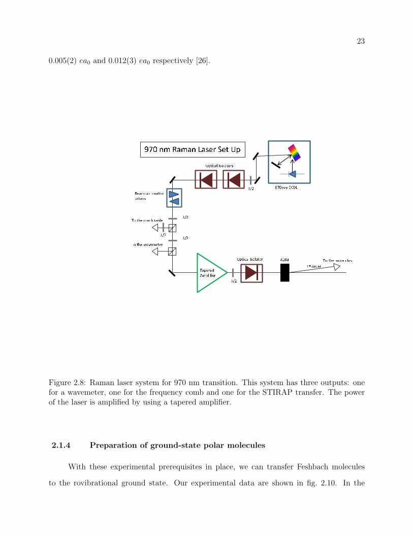
23

0.005(2) ea0 and 0.012(3) ea0 respectively [26].

�� ��� ���� ������ ��� �������� ��� ��������������� ������ ������������ ��������������� ��������� �������

����� �� � � � ! "#$ %#& '()*+ �����

,-. �� /012�� �� ��� ����3����

Figure 2.8: Raman laser system for 970 nm transition. This system has three outputs: onefor a wavemeter, one for the frequency comb and one for the STIRAP transfer. The powerof the laser is amplified by using a tapered amplifier.

2.1.4 Preparation of ground-state polar molecules

With these experimental prerequisites in place, we can transfer Feshbach molecules

to the rovibrational ground state. Our experimental data are shown in fig. 2.10. In the

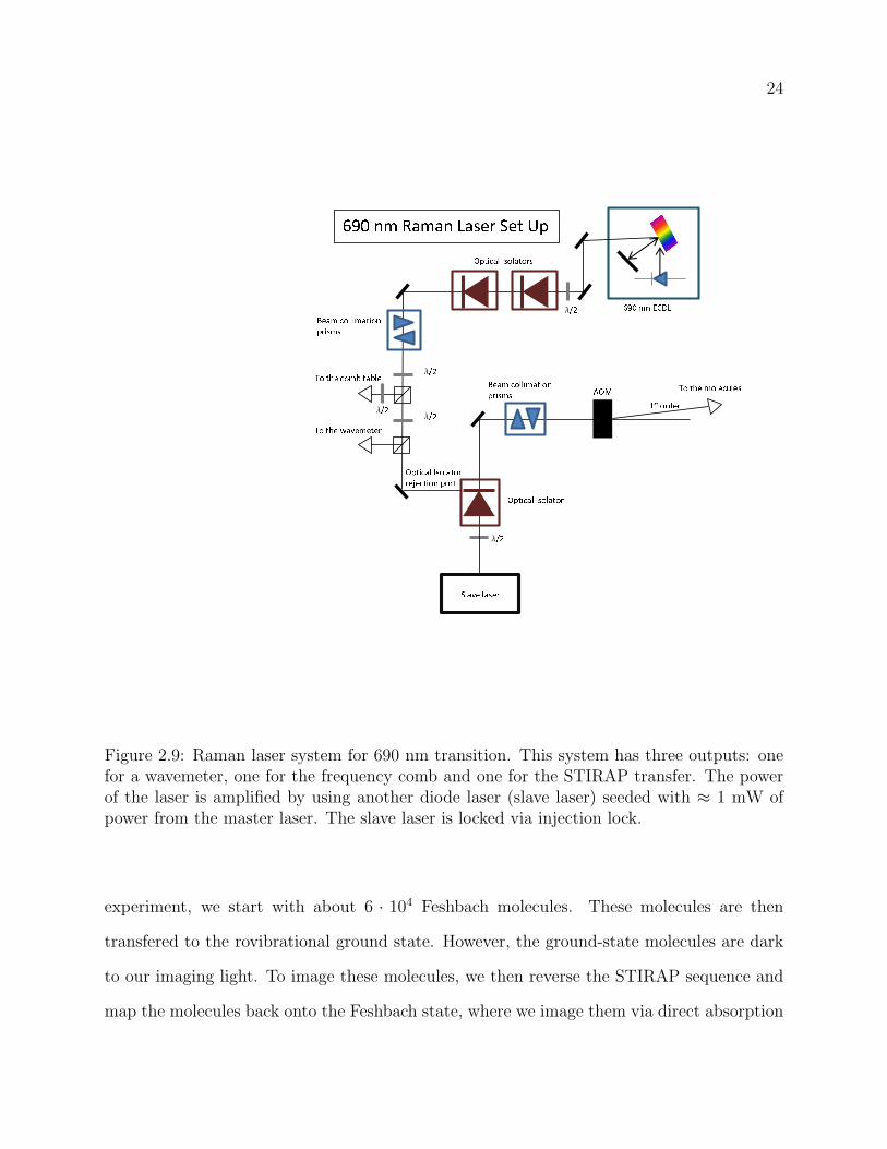
24

�� ��� ���� ������ ��� �������� ��� ��������������� ������ ������������ ��������� �������

����� �� ����� �� !" #!$ %&'() ��*��+,- �� ./01

���� ��� ����2���� ������ ���������3������ ���� 4��� ����

��� ���������������

Figure 2.9: Raman laser system for 690 nm transition. This system has three outputs: onefor a wavemeter, one for the frequency comb and one for the STIRAP transfer. The powerof the laser is amplified by using another diode laser (slave laser) seeded with ≈ 1 mW ofpower from the master laser. The slave laser is locked via injection lock.

experiment, we start with about 6 · 104 Feshbach molecules. These molecules are then

transfered to the rovibrational ground state. However, the ground-state molecules are dark

to our imaging light. To image these molecules, we then reverse the STIRAP sequence and

map the molecules back onto the Feshbach state, where we image them via direct absorption

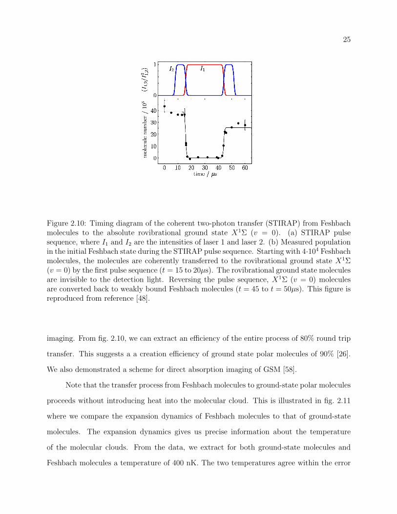
25

Figure 2.10: Timing diagram of the coherent two-photon transfer (STIRAP) from Feshbachmolecules to the absolute rovibrational ground state X1Σ (v = 0). (a) STIRAP pulsesequence, where I1 and I2 are the intensities of laser 1 and laser 2. (b) Measured populationin the initial Feshbach state during the STIRAP pulse sequence. Starting with 4·104 Feshbachmolecules, the molecules are coherently transferred to the rovibrational ground state X1Σ(v = 0) by the first pulse sequence (t = 15 to 20µs). The rovibrational ground state moleculesare invisible to the detection light. Reversing the pulse sequence, X1Σ (v = 0) moleculesare converted back to weakly bound Feshbach molecules (t = 45 to t = 50µs). This figure isreproduced from reference [48].

imaging. From fig. 2.10, we can extract an efficiency of the entire process of 80% round trip

transfer. This suggests a a creation efficiency of ground state polar molecules of 90% [26].

We also demonstrated a scheme for direct absorption imaging of GSM [58].

Note that the transfer process from Feshbach molecules to ground-state polar molecules

proceeds without introducing heat into the molecular cloud. This is illustrated in fig. 2.11

where we compare the expansion dynamics of Feshbach molecules to that of ground-state

molecules. The expansion dynamics gives us precise information about the temperature

of the molecular clouds. From the data, we extract for both ground-state molecules and

Feshbach molecules a temperature of 400 nK. The two temperatures agree within the error

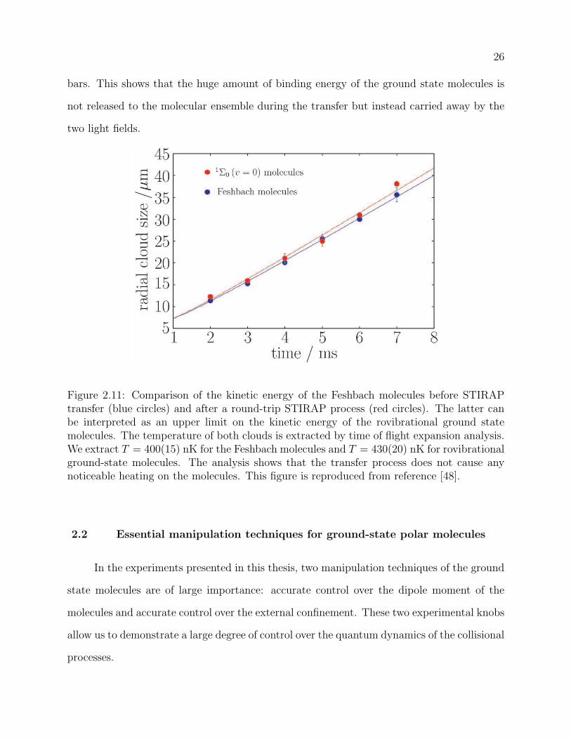
26

bars. This shows that the huge amount of binding energy of the ground state molecules is

not released to the molecular ensemble during the transfer but instead carried away by the

two light fields.

Figure 2.11: Comparison of the kinetic energy of the Feshbach molecules before STIRAPtransfer (blue circles) and after a round-trip STIRAP process (red circles). The latter canbe interpreted as an upper limit on the kinetic energy of the rovibrational ground statemolecules. The temperature of both clouds is extracted by time of flight expansion analysis.We extract T = 400(15) nK for the Feshbach molecules and T = 430(20) nK for rovibrationalground-state molecules. The analysis shows that the transfer process does not cause anynoticeable heating on the molecules. This figure is reproduced from reference [48].

2.2 Essential manipulation techniques for ground-state polar molecules

In the experiments presented in this thesis, two manipulation techniques of the ground

state molecules are of large importance: accurate control over the dipole moment of the

molecules and accurate control over the external confinement. These two experimental knobs

allow us to demonstrate a large degree of control over the quantum dynamics of the collisional

processes.

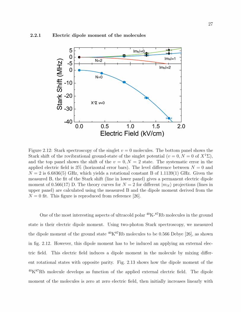
27

2.2.1 Electric dipole moment of the molecules

Figure 2.12: Stark spectroscopy of the singlet v = 0 molecules. The bottom panel shows theStark shift of the rovibrational ground-state of the singlet potential (v = 0, N = 0 of X1Σ),and the top panel shows the shift of the v = 0, N = 2 state. The systematic error in theapplied electric field is 3% (horizontal error bars). The level difference between N = 0 andN = 2 is 6.6836(5) GHz, which yields a rotational constant B of 1.1139(1) GHz. Given themeasured B, the fit of the Stark shift (line in lower panel) gives a permanent electric dipolemoment of 0.566(17) D. The theory curves for N = 2 for different |mN〉 projections (lines inupper panel) are calculated using the measured B and the dipole moment derived from theN = 0 fit. This figure is reproduced from reference [26].

One of the most interesting aspects of ultracold polar 40K-87Rb molecules in the ground

state is their electric dipole moment. Using two-photon Stark spectroscopy, we measured

the dipole moment of the ground state 40K87Rb molecules to be 0.566 Debye [26], as shown

in fig. 2.12. However, this dipole moment has to be induced an applying an external elec-

tric field. This electric field induces a dipole moment in the molecule by mixing differ-

ent rotational states with opposite parity. Fig. 2.13 shows how the dipole moment of the

40K87Rb molecule develops as function of the applied external electric field. The dipole

moment of the molecules is zero at zero electric field, then initially increases linearly with

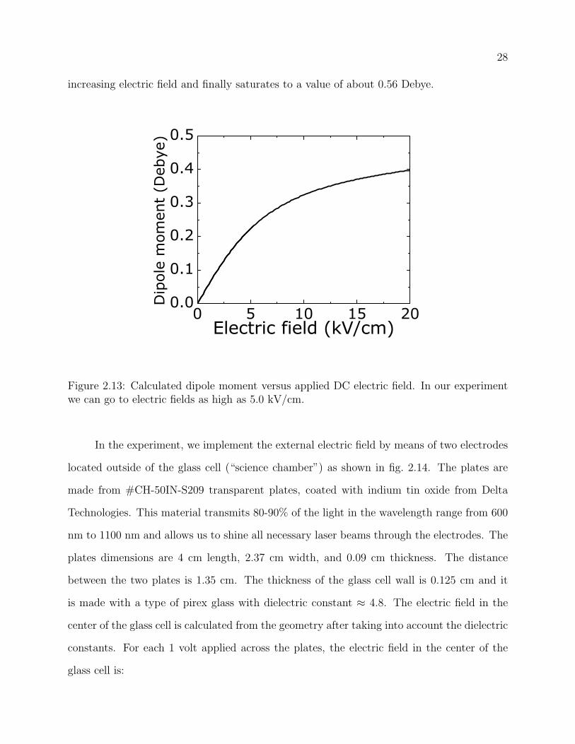
28

increasing electric field and finally saturates to a value of about 0.56 Debye.

0 5 10 15 200.0

0.1

0.2

0.3

0.4

0.5

Dip

ole

mom

ent

(Deb

ye)

Electric field (kV/cm)

Figure 2.13: Calculated dipole moment versus applied DC electric field. In our experimentwe can go to electric fields as high as 5.0 kV/cm.

In the experiment, we implement the external electric field by means of two electrodes

located outside of the glass cell (“science chamber”) as shown in fig. 2.14. The plates are

made from #CH-50IN-S209 transparent plates, coated with indium tin oxide from Delta

Technologies. This material transmits 80-90% of the light in the wavelength range from 600

nm to 1100 nm and allows us to shine all necessary laser beams through the electrodes. The

plates dimensions are 4 cm length, 2.37 cm width, and 0.09 cm thickness. The distance

between the two plates is 1.35 cm. The thickness of the glass cell wall is 0.125 cm and it

is made with a type of pirex glass with dielectric constant ≈ 4.8. The electric field in the

center of the glass cell is calculated from the geometry after taking into account the dielectric

constants. For each 1 volt applied across the plates, the electric field in the center of the

glass cell is:

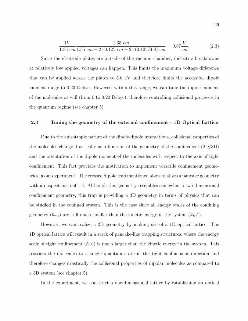
29

1V

1.35 cm

1.35 cm

1.35 cm− 2 · 0.125 cm + 2 · (0.125/4.8) cm= 0.87

V

cm. (2.3)

Since the electrode plates are outside of the vacuum chamber, dielectric breakdowns

at relatively low applied voltages can happen. This limits the maximum voltage difference

that can be applied across the plates to 5.6 kV and therefore limits the accessible dipole

moment range to 0.20 Debye. However, within this range, we can tune the dipole moment

of the molecules at will (from 0 to 0.20 Debye), therefore controlling collisional processes in

the quantum regime (see chapter 5).

2.3 Tuning the geometry of the external confinement - 1D Optical Lattice

Due to the anisotropic nature of the dipole-dipole interactions, collisional properties of

the molecules change drastically as a function of the geometry of the confinement (2D/3D)

and the orientation of the dipole moment of the molecules with respect to the axis of tight

confinement. This fact provides the motivation to implement versatile confinement geome-

tries in our experiment. The crossed dipole trap mentioned above realizes a pancake geometry

with an aspect ratio of 1:4. Although this geometry resembles somewhat a two-dimensional

confinement geometry, this trap is providing a 3D geometry in terms of physics that can

be studied in the confined system. This is the case since all energy scales of the confining

geometry (~ωz) are still much smaller than the kinetic energy in the system (kBT ).

However, we can realize a 2D geometry by making use of a 1D optical lattice. The

1D optical lattice will result in a stack of pancake-like trapping structures, where the energy

scale of tight confinement (~ωz) is much larger than the kinetic energy in the system. This

restricts the molecules to a single quantum state in the tight confinement direction and

therefore changes drastically the collisional properties of dipolar molecules as compared to

a 3D system (see chapter 5).

In the experiment, we construct a one-dimensional lattice by establishing an optical

30

1064 nm light

from Verdi laser

Photo detector

for intensity

stabilizationLens f=50 cm

Lens f=50 cm

Positive

E-field plate

Negative

E-field plate

Glass cell

Optical Table

Breadboard

gravity

/2

1 cm1.35 cm

20

><

>< >

Mirror with

~2% transmition

Figure 2.14: Schematic figure of the electric field plates and 1D optical lattice set up. Themaximum output power of the fiber is 1.7 W. The polarization is set to be parallel to theoptical table. The intensity of the optical lattice is stabilized via an AOM, which also shiftsthe frequency by +80 MHz.

standing wave. A schematic figure of the optical lattice’s experimental set up is shown in

fig. 2.14. The optical lattice potential will then divide the cloud in the optical dipole trap

into a series of pancakes with tight confinement along the vertical z axis (in the gravity

direction). The optical lattice is realized by a single retroreflected laser beam. The beam

waist of the optical lattice matches the beam waist of the dipole optical trap, in order to

avoid heating as the intensity of the optical lattice is ramped up. The beam waist of the

optical lattice is 250 µm. For the optical lattice we use a single-mode Verdi-IR laser with

31

wavelength of 1064 nm, and power up to 25 W. We send light via a polarization-maintaining

optical fiber with coupling efficiency of 40 to 50 %. At the output of the optical fiber, we

get a maximum power of 1.7 W going to the molecules. The laser beam passes through the

electric-field plates and the glass cell and then is reflected back, forming the optical lattice

potential inside the cell. Due to losses in the electric field plates and the glass cell (the glass

cell in not AR coated), the beam power after the rectroreflection is 40 % lower than the

initial power. The optical lattice beam is tilted from the vertical direction by an angle of 2

degrees to avoid back reflections inside of the glass cell impinging the molecular cloud and

causing corrugations in the potential. The stabilization of the optical lattice depth is done

by controlling the laser beam intensity. Approximately 2 % of the light leaks through the

retroreflection mirror. This light is detected and sent to a servo that feeds back to an AOM

that controls the amount of light going to the optical fiber.

Chapter 3

Dipolar 40K87Rb Molecules in 3D geometry

The preparation of a near quantum degenerate gas of all ground-state polar molecules

opens tremendous opportunities for the study and control of molecular collisions in the limit

of vanishing collisional energy. For chemically reactive molecules such as 40K87Rb, it opens

the unique opportunity to study chemical reaction dynamics in the completely unexplored

limit where both the internal quantum states and external quantum states of motion are

well defined. In this regime, collisions can be analyzed by simple quantum mechanical rules

such as quantum statistics, single partial wave scattering, and quantum threshold laws.

In this chapter, I present the studies of ultracold chemical reactions in the quantum

gas of polar molecules when molecules are confined in a 3D geometry as background mate-

rial for my thesis work. These studies were already discussed in the thesis work of K.-K.

Ni [21]. Starting with an optically trapped near-quantum-degenerate ( TTF≈ 1.4) gas of polar

40K87Rb molecules prepared in their absolute ground state, we observe experimental ev-

idence for exothermic atom-exchange chemical reactions. When these fermionic molecules

are prepared in a single quantum state at a temperature of a few hundred nanokelvin, we

observe p-wave dominated quantum threshold collisions arising from tunneling through an

angular momentum barrier followed by a short-range chemical reaction with a probability

near unity. When these molecules were prepared in two different internal states, the reaction

rates were enhanced by a factor of 10 to 100 as a result of s-wave scattering, which does not

have a centrifugal barrier. Inducing an electric dipole moment in the molecules results in

33

tuning of the chemical reaction rate over several orders of magnitudes. Finally, I present the

thermodynamics of the molecular cloud under the influence of strong collisional loss revealing

the anisotropic nature of the dipolar interaction. Throughout this chapter, I closely follow

references [39, 40], which describe our work.

3.1 Bimolecular chemical reactions at ultracold temperature

Molecular quantum gases of 40K87Rb molecules offer the unprecedented opportunity

to study chemical reactions in the limit of vanishing collisional energy. 40K87Rb molecules

are not stable against atom exchange chemical reactions. Two 40K87Rb molecules collide

and form with a high probability different chemical species, namely K2 and Rb2 [39]. This is

because the chemical reactions KRb+KRb→K2+Rb2 is exothermic and moreover proceeds

without chemical reaction barrier at short range [39].

However, chemical reactions have never been studied in the limit of vanishing colli-

sional energy. Even basic questions such as how a chemical reaction proceeds at ultralow

temperature and what quantum mechanical rules are responsible for molecular reactivity

have never been addressed.

That chemical reactions could occur at ultralow temperatures seems at first glance

counterintuitive. However, ultracold collisions, where particles scatter only in the partial

wave with lowest angular momentum, are governed by quantum statistics and quantum

threshold behaviors described by the Bethe-Wigner laws [59, 60]. In this regime, particles

are represented by their de Broglie wavelength, which increases with reduced temperature.

This wave nature of particles replaces our intuitive classical picture of collisions. The wave

manifestation of tunneling through reaction or angular momentum barriers may play a domi-

nant role in dynamics, and scattering resonances can have dramatic effects on reactions [61].

In addition, any barrierless chemical reactions will always take place when two reactants

are sufficiently close together [62]. In this case, chemical reaction rates will be determined

to a large extent by collisional properties at large intermolecular separations, and thus by

34

how the two molecules approach each other. Once their separation reaches a characteristic

length scale ( 10a0, where a0 = 0.53 · 10−10 m), a chemical reaction happens with a near

unity probability. Therefore, chemical reactions can be surprisingly efficient even at ultralow

temperatures. Indeed, this model for barrierless reactions predicts loss rates that are univer-

sal in the sense that they do not depend on the details of the short-range interactions, but

instead can be estimated using only knowledge of the long-range interactions [63].

3.2 The role of quantum statistics in determining the chemical reaction rate

For molecules prepared at a temperature of a few hundred nanokelvin, the collision rate

is largely determined by the quantum statistics of the molecular ensemble. In the regime of

vanishing collisional energy, collisions proceed in a single partial wave, because higher order

angular momentum scattering channels are frozen out due to large centrifugal barriers. This

means that depending on quantum statistics, molecules will collide in an s-wave L = 0

or p-wave L = 1 angular momentum scattering channel. In our experiments, we prepare

fermionic 40K87Rb molecules. For spin-polarized molecules all prepared in the same internal

quantum state, the p-wave collisional channel is then the lowest energy symmetry-allowed

collision channel. The height of the centrifugal barrier for the p-wave (L = 1) KRb-KRb

collision is kB · 24 µK. It is determined by the molecule-molecules long-range potential:

VLongRange(R) =~2L(L + 1)

2µR2− C6

R6, (3.1)

where L = 1, µ is the reduced mass of the 40K87Rb and C6 = 16, 130Eh · a60 (a.u.) [64],

where Eh = 4.36 ·10−18 J. This barrier height is more than an order of magnitude larger than

kBT , where T is the translational temperature of the molecular gas. Thus, collisions of spin

polarized molecules are expected to proceed predominantly via tunneling through the p-wave

barrier. If two molecules make it through the barrier to short range, chemical reactions or

hyperfine state-changing collisions can take place, leading to a loss of the entrance channel

population. We note that even a single nuclear spin flip corresponds to a released quantity of

35

energy that is above the trap depth, and this would contribute to loss of trapped molecules.

Preparing a 50:50 mixture of two different spin states allows molecules to collide in an s-wave

collisional channel. Thus, there is no centrifugal energy barrier and chemical reactions will

therefore proceed at a much higher rate.

3.3 The experimental system

To study chemical reactions of molecules in the quantum regime, we prepare a gaseous

molecular sample at densities on the order of 1012 to 1013 cm−3 and temperatures of around

200 to 300 nK. The fermionic 40K87Rb molecules are prepared in a single hyperfine level of

the rovibronic ground state (N = 0, v = 0 of X1Σ+) [26, 65] and in particular in the absolute

lowest internal quantum state. At the ultralow temperature of a few hundred nK, even the

tiny molecular hyperfine-state energy splitting of ≈ 760 kHz at B = 545.9 G [65], is much

larger than the translational energy (300 nK corresponds to 6 kHz). The preparation of

a well-defined hyperfine state is possible and is of essential importance for the experiments

presented in this chapter. Complete control over the internal quantum state of the molecules

(including hyperfine quantum degrees of freedom) permits direct observation of the role of

quantum statistics in determining the molecular interactions and the chemical reaction rate.

Details on the precise and coherent manipulation of the molecular population in dif-

ferent hyperfine states of the rovibrational ground state X1Σ+ of 40K87Rb can be found

in [65]. The X1Σ+ state has zero total electronic angular momentum, so that the hyperfine

structure is basically the Zeeman effect of the nuclear spins IK = 4 and IRb = 3/2 [63, 66]

at the applied magnetic field. The hyperfine structure is depicted in fig. 3.1, where a total

of 36 states are labeled by their projections of the nuclear spins of 87Rb , mRbI and 40K , mK

I

onto the external magnetic field. For the study of chemical reactions, we produce molecules

either in a single spin state∣∣mK

I ,mRbI

⟩, or in a mixture of two spin states. The hyperfine

states used are an excited state |−4, 1/2〉 and the lowest-energy spin state |−4, 3/2〉. These

are marked by the two ellipses in fig. 3.1. The |−4, 1/2〉 state is populated directly by the

36

two-photon Raman transfer starting from Feshbach molecules [26, 65]. The spin state of

these molecules can be further manipulated coherently. For example, the entire |−4, 1/2〉population can be transferred into the lowest hyperfine state, |−4, 3/2〉, using two successive

microwave π-pulses through a rotationally excited N = 1 intermediate level as shown in

fig. 3.2. Within the N = 1 manifold, coupling between rotation and the nuclear electric

quadrupole moment of 87Rb or 40K atoms lead to mixing of different nuclear spin characters.

Due to this mixing, it is possible to use the rotationally excited state as a bridge between

different hyperfine states in the rotational ground state [65, 66]. We can probe molecules

in any particular hyperfine state by reversing the entire transfer process and putting the

population back into the initial weakly bound state. We use absorption imaging to measure

the molecular gas number and temperature. Alternatively, we can also do direct image of

ground state molecules by using a open optical transition [58].

3.4 Bimolecular chemical reactions at vanishing dipole moment

In first experiments, we studied the chemical reaction KRb+KRb → K2+Rb2 in the

limit of vanishing electric field. In this limit, the 40K87Rb molecules do not have an electric

dipole moment in the lab frame. The long-range interaction potential between two molecules

is then entirely set by the competition between the attractive van-der-Waals interaction and

the centrifugal barrier of the collisional process. Since the centrifugal barrier depends on L,

the quantum statistics of the molecules has a important role for the long range interaction

potential.

3.4.1 p-wave collisions

When the molecules are prepared in a single hyperfine state within the rotational and

vibrational ground state, they are indistinguishable from each other. Since these molecules

are fermions, the collision can only happen through odd angular momentum channels. In the

limit of vanishing collisional energy, the dominating collisional channel is then the p-wave

37

Figure 3.1: Hyperfine structure of rovibronic ground-state 40K87Rb molecules at a magneticfield of 545.9 G. Here we have 36 nuclear spin states by their spin projections, mRb

I and mKI .

The energy spacing between hyperfine states is h · 130 kHz for∣∣mK

I

∣∣ = 1 and h · 760 kHzfor

∣∣mRbI

∣∣ = 1. By comparison, at a temperature of 300 nK, the molecules thermal energy isequivalent to h · 6 kHz, which is more than an order of magnitude smaller than the spin flipenergy. Molecules can be prepared in either a single state or in a mixture of The |−4, 1/2〉and the lowest-energy state |−4, 3/2〉 (open ellipses). Figure reproduced from reference [39].

collisional channel and the competition between the van-der-Waals interaction and the finite

centrifugal energy, which results in a p-wave collisional barrier given by eq. 3.1, with the

angular momentum L = 1 for p-wave collisions. Here C6 = 16, 130 a.u. [64], and the height

of the centrifugal barrier is 24 µK.

As the collisional energy of molecules is in the sub µK regime, and much smaller than

the height of the centrifugal barrier, chemical reactions can only proceed through quantum

mechanical tunneling through the p-wave barrier. On the other hand, once molecules get

within short range of each other, chemical reactions proceed with near-unity probability [41,

67]. We therefore expect the chemical reaction rate to be set by the tunneling rate of the

molecules through the p-wave barrier.

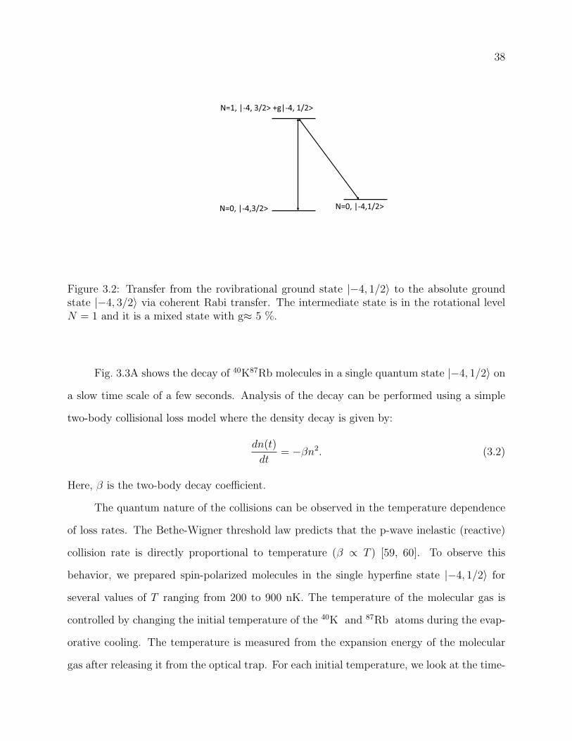
38

N=0, |-4,3/2>

N=1, |-4, 3/2>

N=0, |-4,1/2>

+g|-4, 1/2>

Figure 3.2: Transfer from the rovibrational ground state |−4, 1/2〉 to the absolute groundstate |−4, 3/2〉 via coherent Rabi transfer. The intermediate state is in the rotational levelN = 1 and it is a mixed state with g≈ 5 %.

Fig. 3.3A shows the decay of 40K87Rb molecules in a single quantum state |−4, 1/2〉 on

a slow time scale of a few seconds. Analysis of the decay can be performed using a simple

two-body collisional loss model where the density decay is given by:

dn(t)

dt= −βn2. (3.2)

Here, β is the two-body decay coefficient.

The quantum nature of the collisions can be observed in the temperature dependence

of loss rates. The Bethe-Wigner threshold law predicts that the p-wave inelastic (reactive)

collision rate is directly proportional to temperature (β ∝ T ) [59, 60]. To observe this

behavior, we prepared spin-polarized molecules in the single hyperfine state |−4, 1/2〉 for

several values of T ranging from 200 to 900 nK. The temperature of the molecular gas is

controlled by changing the initial temperature of the 40K and 87Rb atoms during the evap-

orative cooling. The temperature is measured from the expansion energy of the molecular

gas after releasing it from the optical trap. For each initial temperature, we look at the time-

39

dependent molecular loss and extract a two-body loss rate β (which is twice the collisional

event rate) by fitting the decay of the molecular gas density n versus time t (fig. 3.3a) to

dn

dt= −βn2 − αn. (3.3)

Here, the first term on the right takes into account the number loss and the measured β

can be compared to theoretical predictions. The second term allows density change due

to heating of the trapped gas during the measurement. Within a single measurement, we

observe an increase in temperature that is at most 30%. In the analysis for each data set,

we fit the measured temperature to a linear heating rate and obtain a constant slope c. In

eq. 3.3, α = (3/2)[c/(T + ct)], where T is the initial temperature. At the lowest temperature

that we can reach, 250 nK, the heating was (7±1) nK s−1 and β = (3.3±0.7)· 10−12 cm3

s−1. The measured dependence of β versus T is summarized in fig. 3.3b (solid circles).

Here, we fit the data to a power law β(T ) ∝ TL and find that L = 1.1(±0.2), which agrees

with the predicted p-wave threshold law. This result demonstrates that indistinguishable

40K87Rb molecules at ultralow temperatures collide via tunneling through a p-wave barrier

followed by an inelastic collision in the short range. A linear fit to the data (L = 1) yields a

slope of the decay rate coefficient of (1.2± 0.3) · 10−5 cm3 s−1 K−1.

We repeated this measurement for molecules in the lowest hyperfine state |−4, 3/2〉(open triangles in fig. 3.3b). The data again show β ∝ T with a slope of (1.1 ± 0.3) · 10−5

cm3 s−1 K−1, similar to that measured for molecules in the |−4, 1/2〉 state. However, in the

case of |−4, 3/2〉 molecules, hyperfine state-changing collisions are no longer possible and the

only possible loss channels are the chemical reactions discussed above. Thus, we find that

the rate of chemical reactions is determined by the p-wave angular momentum barrier, and

the chemical reaction barrier must be below the collision energy. This suggests that these

reactions are barrierless and can thus occur freely at ultralow temperatures. Meanwhile,

the fact that the same loss rate is observed for both |−4, 1/2〉 and |−4, 3/2〉 state molecules

suggests that chemical reactions dominate the loss in these ground-state molecular collisions.

40

In order to understand the loss rates, two models are used: a quantum threshold

model (QT) [41], and a model that uses the formalism of multichannel quantum defect

theory (MQDT) [67]. In the QT model, the loss rate for collisions with energy equal to

or above the height of the p-wave barrier is determined by the Langevin capture rate [68],

which assumes that the probability for chemical reactions and/or hyperfine state-changing

collisions is unity. For collision energies lower than the height of the p-wave barrier, in

this model we assume that the loss follows the Bethe-Wigner threshold law [59, 60]. Using

this assumption, we have a analytical expression for the p-wave loss rate coefficient of two

indistinguishable molecules, which scales linearly with T [41]:

β =π

4

(317µ3C3

6

~10

)kBT, (3.4)

where µ is the reduced mass. Using a van der Waals dispersion coefficient of C6 = 16, 130 a.u.

for KRb-KRb with an uncertainty of ±10%, the slope of the rate coefficient is predicted to

be 1.5(±0.1)·10−5cm3s−1K−1, which agrees well with the experimental data.

In the MQDT model, the loss rate coefficient is calculated directly by the quantum

tunneling rate through the p-wave barrier [69]. From this calculation β = 0.8(±0.1) · 10−5

cm3s−1K−1, which agrees with the experiment within mutual uncertainties. This β can also

be derived analytically from the properties of the long-range potential to give β = (11.48a)3

(kBT/h), where a = 0.4778(2µC6/~2)1/4 = 6.3 nm is the characteristic length of the van

der Waals potential [63]. This fully quantum calculation can be put in the same form

as the QT model (eq. 3.4) and gives a β that is smaller by a factor of 0.528. With two

models, the agreement with our molecule-molecule collisional loss measurements suggests

that the chemical reaction rates are strongly influenced by the long-range interactions. This

observation opens intriguing control possibilities because the long-range interaction can be

controlled by selecting quantum states and tuning collision energies via applied electric and

magnetic fields.

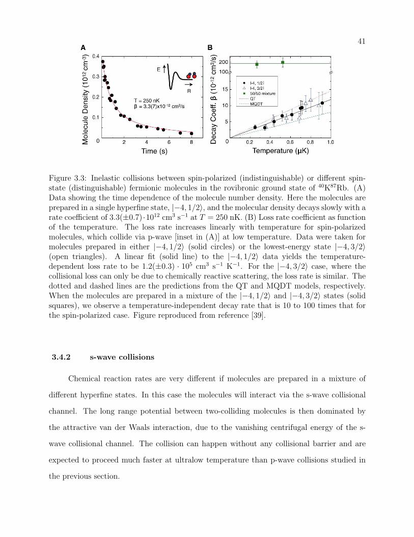
41

Figure 3.3: Inelastic collisions between spin-polarized (indistinguishable) or different spin-state (distinguishable) fermionic molecules in the rovibronic ground state of 40K87Rb. (A)Data showing the time dependence of the molecule number density. Here the molecules areprepared in a single hyperfine state, |−4, 1/2〉, and the molecular density decays slowly with arate coefficient of 3.3(±0.7) ·1012 cm3 s−1 at T = 250 nK. (B) Loss rate coefficient as functionof the temperature. The loss rate increases linearly with temperature for spin-polarizedmolecules, which collide via p-wave [inset in (A)] at low temperature. Data were taken formolecules prepared in either |−4, 1/2〉 (solid circles) or the lowest-energy state |−4, 3/2〉(open triangles). A linear fit (solid line) to the |−4, 1/2〉 data yields the temperature-dependent loss rate to be 1.2(±0.3) · 105 cm3 s−1 K−1. For the |−4, 3/2〉 case, where thecollisional loss can only be due to chemically reactive scattering, the loss rate is similar. Thedotted and dashed lines are the predictions from the QT and MQDT models, respectively.When the molecules are prepared in a mixture of the |−4, 1/2〉 and |−4, 3/2〉 states (solidsquares), we observe a temperature-independent decay rate that is 10 to 100 times that forthe spin-polarized case. Figure reproduced from reference [39].

3.4.2 s-wave collisions

Chemical reaction rates are very different if molecules are prepared in a mixture of

different hyperfine states. In this case the molecules will interact via the s-wave collisional

channel. The long range potential between two-colliding molecules is then dominated by

the attractive van der Waals interaction, due to the vanishing centrifugal energy of the s-

wave collisional channel. The collision can happen without any collisional barrier and are

expected to proceed much faster at ultralow temperature than p-wave collisions studied in

the previous section.

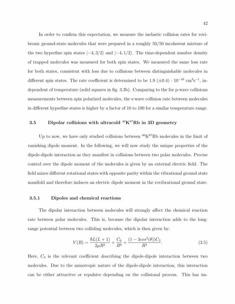
42

In order to confirm this expectation, we measure the inelastic collision rates for rovi-

bronic ground-state molecules that were prepared in a roughly 50/50 incoherent mixture of

the two hyperfine spin states |−4, 3/2〉 and |−4, 1/2〉. The time-dependent number density

of trapped molecules was measured for both spin states. We measured the same loss rate

for both states, consistent with loss due to collisions between distinguishable molecules in

different spin states. The rate coefficient is determined to be 1.9 (±0.4) · 10−10 cm3s−1, in-

dependent of temperature (solid squares in fig. 3.3b). Comparing to the for p-wave collisions

measurements between spin polarized molecules, the s-wave collision rate between molecules

in different hyperfine states is higher by a factor of 10 to 100 for a similar temperature range.

3.5 Dipolar collisions with ultracold 40K87Rb in 3D geometry

Up to now, we have only studied collisions between 40K87Rb molecules in the limit of

vanishing dipole moment. In the following, we will now study the unique properties of the

dipole-dipole interaction as they manifest in collisions between two polar molecules. Precise

control over the dipole moment of the molecules is given by an external electric field. The

field mixes different rotational states with opposite parity within the vibrational ground state

manifold and therefore induces an electric dipole moment in the rovibrational ground state.

3.5.1 Dipoles and chemical reactions

The dipolar interaction between molecules will strongly affect the chemical reaction

rate between polar molecules. This is, because the dipolar interaction adds to the long-

range potential between two colliding molecules, which is then given by:

V (R) =~L(L + 1)

2µR2+

C6

R6+

(1− 3cos2(θ))C3

R3. (3.5)

Here, C3 is the relevant coefficient describing the dipole-dipole interaction between two

molecules. Due to the anisotropic nature of the dipole-dipole interaction, this interaction

can be either attractive or repulsive depending on the collisional process. This has im-

43

0 200 400 600 800 1000-10

0

10

20

30

Pote

ntial energ

y (

K)

Inter-molecular distance (a0)

p-wave

0 200 400 600 800 1000-10

0

10

20

30

Pote

ntial energ

y (

K)

Inter-molecular distance (a0)

0 200 400 600 800 1000-10

0

10

20

30

Pote

ntial energ

y (

K)

Inter-molecular distance (a0)

Figure 3.4: p-wave barrier for 40K87Rb dipolar collisions “head-to-tail” (solid curve in blue)and “side-by-side” (solid curve in red). The dashed line represents the p-wave in the absenceof electric-field.

portant consequences on the chemical reaction rate for molecular ensembles, as illustrated

in fig. 3.4. Preparing an ensemble of indistinguishable fermionic molecules, molecules will

collide predominantly in the p-wave collisional channel which has a collisional barrier of

24µK. In this case, the dipole-dipole interaction will either reduce or enhance the height of

the collisional barrier, depending on whether collisions are attractive (“head-to-tail” colli-

sions) or repulsive (“side-by-side collisions”). The dependence of the height of the collisional

barrier as a function of the dipole moment of the molecules for both collisional channels

is shown in fig. 3.6c. In the limit of small dipole moments relevant to our experiments,

the collisional barrier will go down with the fourth power of the dipole moment for “head-

to-tail” attractive collisions and will rise with the fourth power of the dipole moment for

repulsive “side-by-side” collisions. We therefore expect the rate of attractive “head-to-tail”

44

collisions to increase dramatically with the dipole moment, whereas we expect at the same

time repulsive “side-by-side” collisions to be strongly suppressed with increasing dipole mo-

ment. In the experiments performed in 3D, we expect the loss mechanism of the interactions

“head-to-tail” to dominate our measurement.

3.5.2 The experiment

In order to study dipole-dipole interactions in collisions between molecules, we prepare

a near quantum degenerate ensemble of 40K87Rb molecules in a single nuclear hyperfine

state |−4, 1/2〉 within the rovibronic ground state. The gas is confined in a pancake-shaped

optical dipolar trap. For this experiment, the harmonic trapping frequencies are ωx =

2π × 40 Hz and ωz = 2π × 280 Hz in the horizontal and vertical directions, respectively.

The 40K87Rb molecules have a permanent electric dipole moment of 0.57 Debye. However,

the effective molecular dipole moment in the laboratory frame is zero in the absence of an

external electric field. When an external electric field is applied, the molecules begin to align

with the field and have an induced dipole moment, d, that increases as shown in the inset of

fig. 3.5b. In our set-up, the external electric field points up (in the z direction), parallel to

the tight axis of the optical dipole trap. Thus, the spatially anisotropic dipolar interactions

will be predominantly repulsive for molecules colliding in the horizontal direction (“side-by-

side”) and predominantly attractive for molecules approaching each other along the vertical

direction (“head-to-tail”). However, the molecular confinement in this pancake shaped trap

is 3D and hence neither of the collisional channel is suppressed.

3.5.3 Controlling chemical reactions by means of the dipole moment of the

molecules

Using a single quantum state fermionic gas of rovibrational ground state polar molecules,

we study the effect of electric dipolar interactions on collisions and find an unexpectedly large

effect even for our relatively modest range of applied electric fields. We measure the molec-

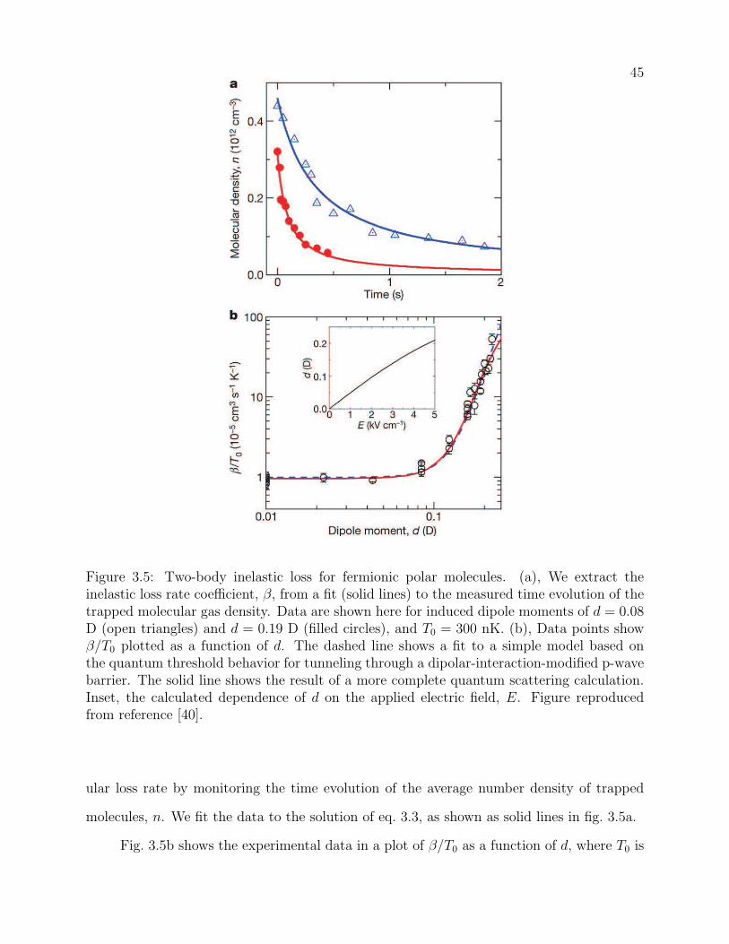
45

Figure 3.5: Two-body inelastic loss for fermionic polar molecules. (a), We extract theinelastic loss rate coefficient, β, from a fit (solid lines) to the measured time evolution of thetrapped molecular gas density. Data are shown here for induced dipole moments of d = 0.08D (open triangles) and d = 0.19 D (filled circles), and T0 = 300 nK. (b), Data points showβ/T0 plotted as a function of d. The dashed line shows a fit to a simple model based onthe quantum threshold behavior for tunneling through a dipolar-interaction-modified p-wavebarrier. The solid line shows the result of a more complete quantum scattering calculation.Inset, the calculated dependence of d on the applied electric field, E. Figure reproducedfrom reference [40].

ular loss rate by monitoring the time evolution of the average number density of trapped

molecules, n. We fit the data to the solution of eq. 3.3, as shown as solid lines in fig. 3.5a.

Fig. 3.5b shows the experimental data in a plot of β/T0 as a function of d, where T0 is

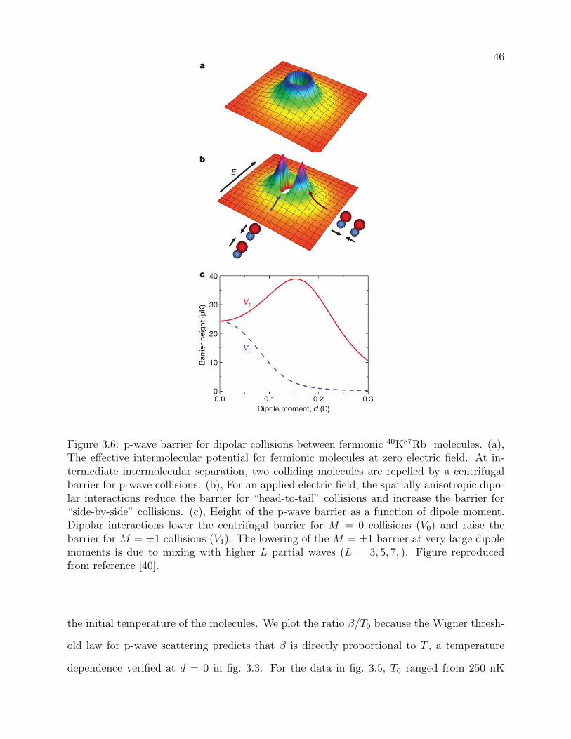
46

Figure 3.6: p-wave barrier for dipolar collisions between fermionic 40K87Rb molecules. (a),The effective intermolecular potential for fermionic molecules at zero electric field. At in-termediate intermolecular separation, two colliding molecules are repelled by a centrifugalbarrier for p-wave collisions. (b), For an applied electric field, the spatially anisotropic dipo-lar interactions reduce the barrier for “head-to-tail” collisions and increase the barrier for“side-by-side” collisions. (c), Height of the p-wave barrier as a function of dipole moment.Dipolar interactions lower the centrifugal barrier for M = 0 collisions (V0) and raise thebarrier for M = ±1 collisions (V1). The lowering of the M = ±1 barrier at very large dipolemoments is due to mixing with higher L partial waves (L = 3, 5, 7, ). Figure reproducedfrom reference [40].

the initial temperature of the molecules. We plot the ratio β/T0 because the Wigner thresh-

old law for p-wave scattering predicts that β is directly proportional to T , a temperature

dependence verified at d = 0 in fig. 3.3. For the data in fig. 3.5, T0 ranged from 250 nK

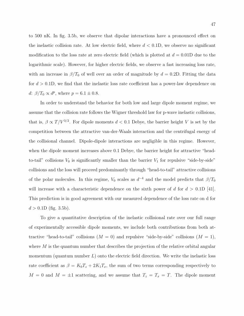
47

to 500 nK. In fig. 3.5b, we observe that dipolar interactions have a pronounced effect on

the inelastic collision rate. At low electric field, where d < 0.1D, we observe no significant

modification to the loss rate at zero electric field (which is plotted at d = 0.01D due to the

logarithmic scale). However, for higher electric fields, we observe a fast increasing loss rate,

with an increase in β/T0 of well over an order of magnitude by d = 0.2D. Fitting the data

for d > 0.1D, we find that the inelastic loss rate coefficient has a power-law dependence on

d: β/T0 ∝ dp, where p = 6.1± 0.8.

In order to understand the behavior for both low and large dipole moment regime, we

assume that the collision rate follows the Wigner threshold law for p-wave inelastic collisions,

that is, β ∝ T/V 3/2. For dipole moments d < 0.1 Debye, the barrier height V is set by the

competition between the attractive van-der-Waals interaction and the centrifugal energy of

the collisional channel. Dipole-dipole interactions are negligible in this regime. However,

when the dipole moment increases above 0.1 Debye, the barrier height for attractive “head-

to-tail” collisions V0 is significantly smaller than the barrier V1 for repulsive “side-by-side”

collisions and the loss will proceed predominantly through “head-to-tail” attractive collisions

of the polar molecules. In this regime, V0 scales as d−4 and the model predicts that β/T0

will increase with a characteristic dependence on the sixth power of d for d > 0.1D [41].

This prediction is in good agreement with our measured dependence of the loss rate on d for

d > 0.1D (fig. 3.5b).

To give a quantitative description of the inelastic collisional rate over our full range

of experimentally accessible dipole moments, we include both contributions from both at-

tractive “head-to-tail” collisions (M = 0) and repulsive “side-by-side” collisions (M = 1),

where M is the quantum number that describes the projection of the relative orbital angular

momentum (quantum number L) onto the electric field direction. We write the inelastic loss

rate coefficient as β = K0Tz + 2K1Tx, the sum of two terms corresponding respectively to

M = 0 and M = ±1 scattering, and we assume that Tz = Tx = T . The dipole moment

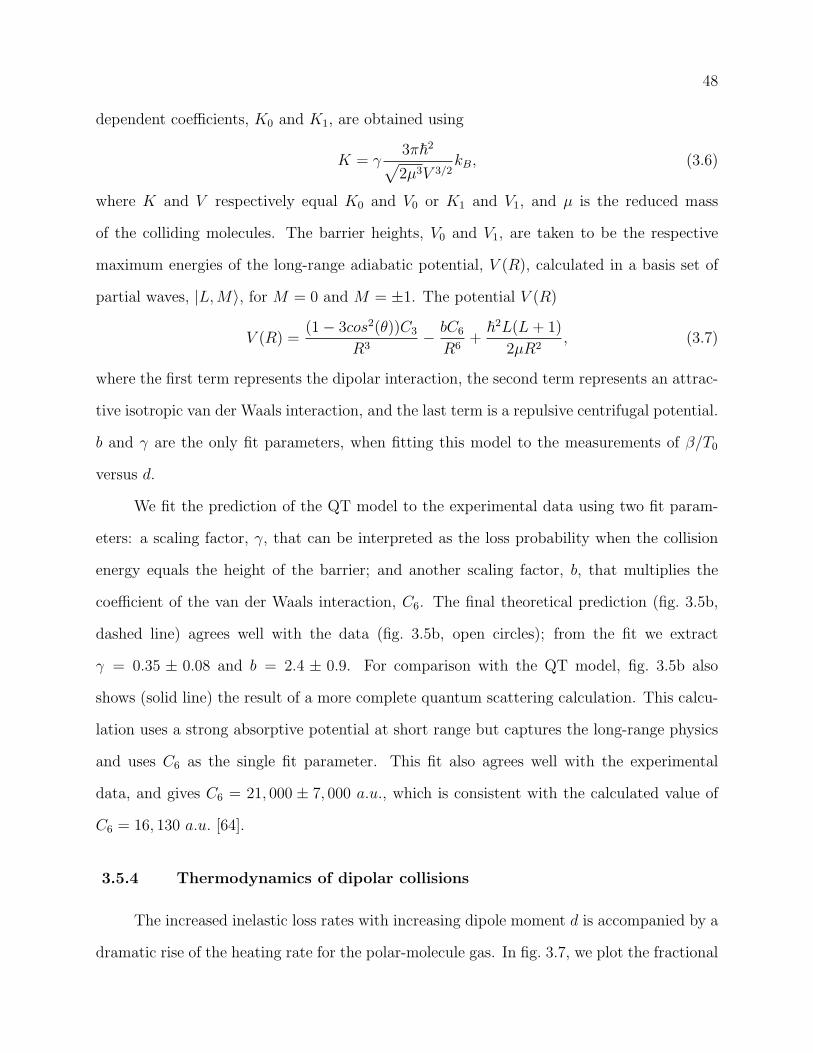
48

dependent coefficients, K0 and K1, are obtained using

K = γ3π~2

√2µ3V 3/2

kB, (3.6)

where K and V respectively equal K0 and V0 or K1 and V1, and µ is the reduced mass

of the colliding molecules. The barrier heights, V0 and V1, are taken to be the respective

maximum energies of the long-range adiabatic potential, V (R), calculated in a basis set of

partial waves, |L,M〉, for M = 0 and M = ±1. The potential V (R)

V (R) =(1− 3cos2(θ))C3

R3− bC6

R6+~2L(L + 1)

2µR2, (3.7)

where the first term represents the dipolar interaction, the second term represents an attrac-

tive isotropic van der Waals interaction, and the last term is a repulsive centrifugal potential.

b and γ are the only fit parameters, when fitting this model to the measurements of β/T0

versus d.

We fit the prediction of the QT model to the experimental data using two fit param-

eters: a scaling factor, γ, that can be interpreted as the loss probability when the collision

energy equals the height of the barrier; and another scaling factor, b, that multiplies the

coefficient of the van der Waals interaction, C6. The final theoretical prediction (fig. 3.5b,

dashed line) agrees well with the data (fig. 3.5b, open circles); from the fit we extract

γ = 0.35 ± 0.08 and b = 2.4 ± 0.9. For comparison with the QT model, fig. 3.5b also

shows (solid line) the result of a more complete quantum scattering calculation. This calcu-

lation uses a strong absorptive potential at short range but captures the long-range physics

and uses C6 as the single fit parameter. This fit also agrees well with the experimental

data, and gives C6 = 21, 000 ± 7, 000 a.u., which is consistent with the calculated value of

C6 = 16, 130 a.u. [64].

3.5.4 Thermodynamics of dipolar collisions

The increased inelastic loss rates with increasing dipole moment d is accompanied by a

dramatic rise of the heating rate for the polar-molecule gas. In fig. 3.7, we plot the fractional

49

heating rate, T /T0, normalized by the initial density n and temperature T0, as a function of

d. The heating rate T = c is extracted using a linear fit to the temperature of the molecular

cloud measured as a function of time over a period sufficiently long to allow T to increase by

approximately 20-30%. We have developed a simple thermodynamic model for heating that is

directly caused by the inelastic loss. We consider the energy lost from the gas when molecules

are removed in inelastic collisions, and assume that the gas stays in thermal equilibrium.

In this model, the heating arises solely from density-dependent loss of particles from the

trap, where the particles removed by inelastic collisions have, on average, lower energies

than typical particles in the gas. This is also called “anti-evaporation” mechanism [70].

One way to understand this anti-evaporation is to note that inelastic collisions preferentially

remove particles from the center of the trap, where the number density is the highest and

the particles have the lowest potential energy from the trap. In our model, we also include a

competing, “cooling”, effect that comes from the fact that the p-wave inelastic collision rate

increases linearly with the collision energy. Including these two competing effects, our model

bassed on the analysis shows that the initial heating rate of the molecules is proportional to

the inelastic loss rate β by a factor of 1/12. When we plot βT0

/12 in fig. 3.7 (solid line) we

can see that our model explains the heating well, where we obtain T 20 n = (β/T0)/12.

3.5.5 Anisotropy of heating

The anisotropy of the dipole-dipole interaction is shown directly in the energy distri-

bution of molecules in the trap. The average energy per particle, which we measure from

the expansion of the gas following a sudden release from the trap, can be different in the

vertical and horizontal directions. In the following, we present measurements of the time

evolution of the expansion energy in these two directions for different values of d. To probe

the spatial anisotropy of dipolar collisions, we start by adding energy along one direction

of the cylindrically symmetric trap using parametric heating. We modulate the power of

both optical trapping beams at twice the relevant harmonic trapping frequency, for 50 ms (z

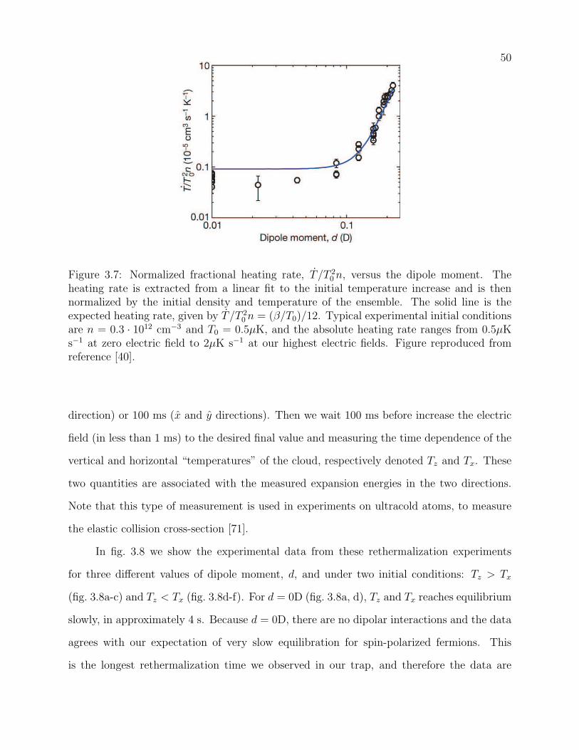
50

Figure 3.7: Normalized fractional heating rate, T /T 20 n, versus the dipole moment. The

heating rate is extracted from a linear fit to the initial temperature increase and is thennormalized by the initial density and temperature of the ensemble. The solid line is theexpected heating rate, given by T /T 2

0 n = (β/T0)/12. Typical experimental initial conditionsare n = 0.3 · 1012 cm−3 and T0 = 0.5µK, and the absolute heating rate ranges from 0.5µKs−1 at zero electric field to 2µK s−1 at our highest electric fields. Figure reproduced fromreference [40].

direction) or 100 ms (x and y directions). Then we wait 100 ms before increase the electric

field (in less than 1 ms) to the desired final value and measuring the time dependence of the

vertical and horizontal “temperatures” of the cloud, respectively denoted Tz and Tx. These

two quantities are associated with the measured expansion energies in the two directions.

Note that this type of measurement is used in experiments on ultracold atoms, to measure

the elastic collision cross-section [71].

In fig. 3.8 we show the experimental data from these rethermalization experiments

for three different values of dipole moment, d, and under two initial conditions: Tz > Tx

(fig. 3.8a-c) and Tz < Tx (fig. 3.8d-f). For d = 0D (fig. 3.8a, d), Tz and Tx reaches equilibrium

slowly, in approximately 4 s. Because d = 0D, there are no dipolar interactions and the data

agrees with our expectation of very slow equilibration for spin-polarized fermions. This

is the longest rethermalization time we observed in our trap, and therefore the data are

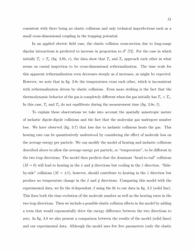
51

consistent with there being no elastic collisions and only technical imperfections such as a

small cross-dimensional coupling in the trapping potential.

In an applied electric field case, the elastic collision cross-section due to long-range

dipolar interactions is predicted to increase in proportion to d4 [72]. For the case in which

initially Tz > Tx (fig. 3.8b, c), the data show that Tz and Tx approach each other in what

seems on casual inspection to be cross-dimensional rethermalization. The time scale for

this apparent rethermalization even decreases steeply as d increases, as might be expected.

However, we note that in fig. 3.8c the temperatures cross each other, which is inconsistent

with rethermalization driven by elastic collisions. Even more striking is the fact that the

thermodynamic behavior of the gas is completely different when the gas initially has Tz < Tx.

In this case, Tz and Tx do not equilibrate during the measurement time (fig. 3.8e, f).

To explain these observations we take into account the spatially anisotropic nature

of inelastic dipole-dipole collisions and the fact that the molecular gas undergoes number

loss. We have observed (fig. 3.7) that loss due to inelastic collisions heats the gas. This

heating rate can be quantitatively understood by considering the effect of molecule loss on

the average energy per particle. We can modify the model of heating and inelastic collisions

described above to allow the average energy per particle, or “temperature”, to be different in

the two trap directions. The model then predicts that the dominant “head-to-tail” collisions

(M = 0) will lead to heating in the x and y directions but cooling in the z direction. “Side-

by-side” collisions (M = ±1), however, should contribute to heating in the z direction but

produce no temperature change in the x and y directions. Comparing this model with the

experimental data, we fix the d-dependent β using the fit to our data in fig. 3.5 (solid line).

This fixes both the time evolution of the molecule number as well as the heating rates in the

two trap directions. Then we include a possible elastic collision effects in the model by adding

a term that would exponentially drive the energy difference between the two directions to

zero. In fig. 3.8 we also present a comparison between the results of the model (solid lines)

and our experimental data. Although the model uses few free parameters (only the elastic

52

collision cross-section, σel, in addition to the initial values of n, Tx and Tz), it provides good

agreement with the experimental data.

Figure 3.8: Cross-dimensional rethermalization in the polar molecule gas. Shown as a func-tion of dipole moment, d, for Tz > Tx (a-c) and Tz < Tx (d-f). The experimental datashows difference between heating the gas in the vertical direction (a-c) and heating it in thehorizontal directions (d-f). This provides evidence for the strong anisotropic characteristicof dipolar interactions. The electric field is applied along the z direction. Figure reproducedfrom reference [40].

The differential equations used as model are shown as it follows. The solid lines in

fig. 3.8 are a fit of the measured time evolution of n, Tz and Tx to the numerical solution of

the following three differential equations [40]:

dn

dt= −(K0Tz + 2K1Tx)n

2 − n

2Tz

dTz

dt− n

Tx

dTx

dt, (3.8)

dTz

dt=

n

4(−K0Tz + 2K1Tx)Tz − 2Γel

3(Tz − Tx) + cbg, (3.9)

dTx

dt=

n

4K0TzTx +

Γel

3(Tz − Tx) + cbg. (3.10)

53

Here we have allowed for a difference in the average energies per particle in the two trap

directions, Tz and Tx. For the fits, we fix the d-dependent coefficients K0 and K1 using the

previous fit to the inelastic loss rate data in fig. 3.5. In addition to heating due to inelastic

loss, we include a measured background heating rate of cbg = 0.01 µK s−1. The elastic colli-

sion rate in eqs. 3.9 and 3.10 is given by Γel = nσelv/Ncoll, where v =√

8kB(Tz + 2Tx)/3πµ

and the constant Ncoll is the mean number of collisions per particle required for rethermal-

ization. We use Ncoll = 4.1, which was computed for p-wave collisions [73]. However, we

note that Ncoll depends on the angular dependence of the scattering and may be different

for dipolar elastic collisions.

Chapter 4

Polar Molecules in an 1D Optical Lattice: Going to 2D Geometry

The anisotropy of the dipolar interaction allows one to control scattering by controlling

the orientation of the molecular dipole moment and the geometry of the external confinement.

In this context, 2D geometries are of particular interest. Orienting the dipole moment of the

molecules along the axis of tight confinement will result in a strong suppression of attractive

“head-to-tail” collisions, if the confinement along that direction is sufficiently strong. This

reduces inelastic scattering events in the molecular gas by a factor of 60 [74] and opens the

path towards the study of long-lived ultracold polar molecular quantum gases and quantum

degenerate molecular ensembles.

In our experiment, we realize a two-dimensional trapping geometry by means of a 1D

optical lattice. This results in a stack of two-dimensional trapping geometries (pancakes)

for the molecules. In this chapter, I will review the well-known concepts of optical dipole

trapping and the realization of a 1D optical lattice. I will discuss how to describe particles

in a periodic potential in terms of Bloch bands or Wannier functions. I will then introduce

basic experimental techniques such as loading of molecular gases into the optical lattice and

characterization techniques such as measurement of the momentum and quasimomentum

distributions of the molecules in the optical lattice. Finally, I will discuss how to prepare

ground-state polar molecules in the 1D optical lattice and how we achieve population control

in selected vibrational levels of the optical lattice.

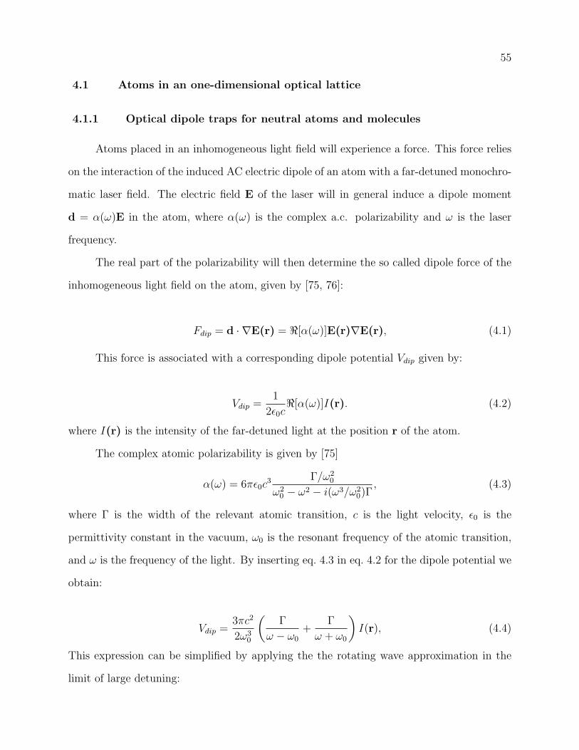
55

4.1 Atoms in an one-dimensional optical lattice

4.1.1 Optical dipole traps for neutral atoms and molecules

Atoms placed in an inhomogeneous light field will experience a force. This force relies

on the interaction of the induced AC electric dipole of an atom with a far-detuned monochro-

matic laser field. The electric field E of the laser will in general induce a dipole moment

d = α(ω)E in the atom, where α(ω) is the complex a.c. polarizability and ω is the laser

frequency.

The real part of the polarizability will then determine the so called dipole force of the

inhomogeneous light field on the atom, given by [75, 76]:

Fdip = d · ∇E(r) = <[α(ω)]E(r)∇E(r), (4.1)

This force is associated with a corresponding dipole potential Vdip given by:

Vdip =1

2ε0c<[α(ω)]I(r). (4.2)

where I(r) is the intensity of the far-detuned light at the position r of the atom.

The complex atomic polarizability is given by [75]

α(ω) = 6πε0c3 Γ/ω2

0

ω20 − ω2 − i(ω3/ω2

0)Γ, (4.3)

where Γ is the width of the relevant atomic transition, c is the light velocity, ε0 is the

permittivity constant in the vacuum, ω0 is the resonant frequency of the atomic transition,

and ω is the frequency of the light. By inserting eq. 4.3 in eq. 4.2 for the dipole potential we

obtain:

Vdip =3πc2

2ω30

(Γ

ω − ω0

+Γ

ω + ω0

)I(r), (4.4)

This expression can be simplified by applying the the rotating wave approximation in the

limit of large detuning:

56

Vdip =3πc2

2ω30

(Γ

∆

)I(r), (4.5)

where ∆ ≡ ω − ω0 is the detuning.

Eq. 4.5 explains the basic physics of dipole trapping in a far-detuned laser field. The

potential scales as I(r)/∆. The potential depth therefore increases linearly with the intensity

of the light field and decreases linearly with increasing detuning of the light field. Whether

the potential is attractive or repulsive depends on the detuning of the light field relative

to the relevant atomic transitions. For red detuned light, ∆ < 0, the dipole potential is

attractive, and for blue detuned light, ∆ > 0, the potential is repulsive.

The simplest configuration for the realization of a confining potential by means of dipole

potentials is therefore a single Gaussian laser beam with a frequency red-detuned from the

relevant atomic transitions and focused down to a spot size of typically about 10-100 µm.

The atoms will then be confined in the focus of this dipole trap with a strong confinement

perpendicular to the axis of propagation of the laser light and a relatively weak confinement

along the axis of propagation.

According to eq. 4.5, the depth of the confining potential is entirely set by the intensity

of the light field and the detuning of the light frequency relative to the atomic transitions.

At first sight, it might therefore seem favorable to operate dipole traps at small detunings to

achieve a maximal depth at low intensity. However, atoms interacting with light fields will

also scatter photon. Photon scattering results in heating of the atomic clouds. The photon

scattering rate is determined by the imaginary part of the polarizability:

Γsc =1

~ε0c=[α(ω)]I(r), (4.6)

This expression can be simplified in a similar formalism as applied above to

Γsc =3πc2

2~ω30

(Γ

∆

)2

I(r). (4.7)

57

As can be seen in eq. 4.7, the scattering rate scales ∝ I(r)/∆2. In particular, the

photon scattering rate decreases much faster with increasing detuning (with the square of

the detuning) as compared the potential depth (decreasing linearly with detuning). It is

therefore favorable to operate optical dipole traps as far detuned as practically possible to

avoid photon scattering processes that lead to heating of the confined atomic ensemble.

For more details please refer to reference [75] by R. Grimm et al.

4.1.2 One-dimensional optical lattice

A one-dimensional (1D) periodic lattice potential can be created by retro-reflecting a

monochromatic laser beam and therefore super-imposing two counter-propagating light fields

with a fixed phase relation with each other. This configuration will result in the formation

of a standing wave with alternating intensity maxima and intensity minima. Neighboring

intensity maxima/minima will be separated by λ/2, where λ is the optical wavelength for

the lattice beam.

In the experiment, the optical lattice will be formed by two counter-propagating Gaus-

sian laser beams with a typical waist of a few hundred µm. The resulting optical potential

is then given by

V (r, z) = V0e−2 r2

w2(z) cos2(kz), (4.8)

where V0 ≡ 8Pαπw2(z)

, P is the laser power, w(z) = w0

√1 + (z/zR)2 is the beam waist at z, w0

is the beam waist at the focus, k = 2π/λ is the wave number, λ is the wavelength of the

laser light, α is the polarizability, and zR = πw20/λ is the Rayleigh length.

For red detuned laser light, the atoms will be trapped in the anti-nodes of the standing

wave (optical lattice), as shown in fig. 4.1. The one-dimensional optical lattice results in a

trapping potential consisting of a stack of pancake-like traps. The confinement perpendicular

to the plane of the pancake is much tighter than the confinement in the plane of the pancake

58

with trapping frequencies given by:

ωr =

√1

m

(∂2V (r, z)

∂r2

)

r,z=0

=

√4Erec

mw20

√V0

Erec

, (4.9)

and

ωz =

√1

m

(∂2V (r, z)

∂z2

)

r,z=0

=2Erec

~

√V0

Erec

, (4.10)

respectively. Here, Erec = ~2k2

2mis the recoil energy associated with the lattice photon. Atoms

in a single pancake are trapped in 2D-geometry if the optical lattice potential is sufficiently

deep.

-4 -2 0 2 4-2

-1

0

1

2

z�Λ

r�w

0

w0 = Λ

01

-4 -2 0 2 4-2

-1

0

1

2

z�Λ

r�w

0

w0 = 250Λ

01

(a) (b)

Figure 4.1: Illustrative contour plot of one-dimensional optical lattice potential. (a) Nor-malized potential in false color for w0 = λ. (b) Potential for w0 = 250λ. The point withmaximum density are the anti-nodes where, for a red-detuned optical lattice, the particleswill be trapped. In our case, the lattice beam waist is w0 ≈ 250µm.

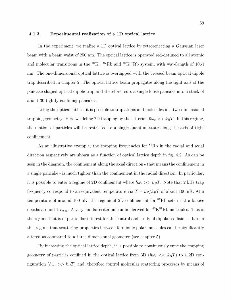
59

4.1.3 Experimental realization of a 1D optical lattice

In the experiment, we realize a 1D optical lattice by retroreflecting a Gaussian laser

beam with a beam waist of 250 µm. The optical lattice is operated red-detuned to all atomic

and molecular transitions in the 40K , 87Rb and 40K87Rb system, with wavelength of 1064

nm. The one-dimensional optical lattice is overlapped with the crossed beam optical dipole

trap described in chapter 2. The optical lattice beam propagates along the tight axis of the

pancake shaped optical dipole trap and therefore, cuts a single loose pancake into a stack of

about 30 tightly confining pancakes.

Using the optical lattice, it is possible to trap atoms and molecules in a two-dimensional

trapping geometry. Here we define 2D trapping by the criterion ~ωz >> kBT . In this regime,

the motion of particles will be restricted to a single quantum state along the axis of tight

confinement.

As an illustrative example, the trapping frequencies for 87Rb in the radial and axial

direction respectively are shown as a function of optical lattice depth in fig. 4.2. As can be

seen in the diagram, the confinement along the axial direction - that means the confinement in

a single pancake - is much tighter than the confinement in the radial direction. In particular,

it is possible to enter a regime of 2D confinement where ~ωz >> kBT . Note that 2 kHz trap

frequency correspond to an equivalent temperature via T = hν/kBT of about 100 nK. At a

temperature of around 100 nK, the regime of 2D confinement for 87Rb sets in at a lattice

depths around 1 Erec. A very similar criterion can be derived for 40K87Rb molecules. This is

the regime that is of particular interest for the control and study of dipolar collisions. It is in

this regime that scattering properties between fermionic polar molecules can be significantly

altered as compared to a three-dimensional geometry (see chapter 5).

By increasing the optical lattice depth, it is possible to continuously tune the trapping

geometry of particles confined in the optical lattice from 3D (~ωz << kBT ) to a 2D con-

figuration (~ωz >> kBT ) and, therefore control molecular scattering processes by means of

60

external confinement.

4.1.4 Quantum mechanical description of a particle confined in a periodic

potential: Bloch bands

The quantum mechanical picture of a particle moving in a periodic potential is a well

known problem. The description of atomic motion is captured by the formalism of Bloch

wavefunctions and Bloch bands [77]. The periodic potential in this case is provided by the

interference pattern of light. A single particle of mass m moving in this periodic potential

V (z) = V0cos2(kz) is described by the time-independent Schrodinger equation:

(− 1

2mp2 + V0cos

2(kz)

)Ψq,n(z) = Eq,nΨq,n(z), (4.11)

where n is the quantum number relative to the internal state of the optical lattice. The

eigenfunctions of this Schrodinger equation are called Bloch waves. These Bloch functions

can be written as the product of the plane waves eiqz/~ with quasimomentum q times an

0 10 20 30 40 50 600

500010 00015 00020 00025 00030 000

V0HErecL

ΝzH

HzL

0 10 20 30 40 50 600

10203040506070

V0HErecL

ΝxH

HzL

(a) (b)

Figure 4.2: Optical lattice’s trap frequencies versus the trap depth for 87Rb . This two plotsshow the axial frequency νz compared to the radial frequency νr. The confinement in theaxial direction is much tighter than the radial direction. The optical lattice parameters are:λ = 1064 nm, and the beam waist is 250 µm.

61

envelope function uq,n(z) with the periodicity of the confining potential:

Ψq,n(z) = eiqz/~uq,n(z). (4.12)

These wavefunctions are delocalized over the whole lattice structure.

Due to the periodicity, we can expand both the external potential and the wavefunctions

in terms of a Fourier sum:

V (z) =∑

j

Vjei2jkz, (4.13)

and

uq,n(z) =∑

l

c(q,n)l ei2lkz. (4.14)

Substituting eq. 4.13 and eq. 4.14 into eq. 4.11 and after some algebraic manipulations, the

Schrodinger equation can be written in a matrix form given by [77]:

{[(2l +

q

~k

)2

Erec − V0

2

]δl,l′ − V0

4δl,l′±1

}c(q,n)l = Eq,nc

(q,n)l , (4.15)

where −~k ≤ q ≤ ~k, limited to the first Brillouin zone. Eq,n represents the eigenenergies of

the nth Bloch band for a given q. The eigenstates c(q,n) are the Bloch wavefunctions.

Note that we have introduced an additional quantum number, the band index n. The

quasimomentum q is unique only up the addition of integer multiples of the reciprocal lattice

vector k. It is therefore convenient to restrict the quasimomenta to the first Brillouin zone

given by−~k < q < ~k. This means that a multiple number of eigenfunctions and eigenstates

exists for a given quasimomentum q. These eigenstates are denoted by the band index n.

Fig. 4.3 shows the energy spectrum of particles confined in optical lattices for various

lattice depths. In the limit of vanishing optical lattice potential, the quasimomentum q is

equal to the free particle momentum and the energy spectrum is given by the free particle

energy dispersion Eq = ~2q2/2m. The band structure in this case appears due to the artificial

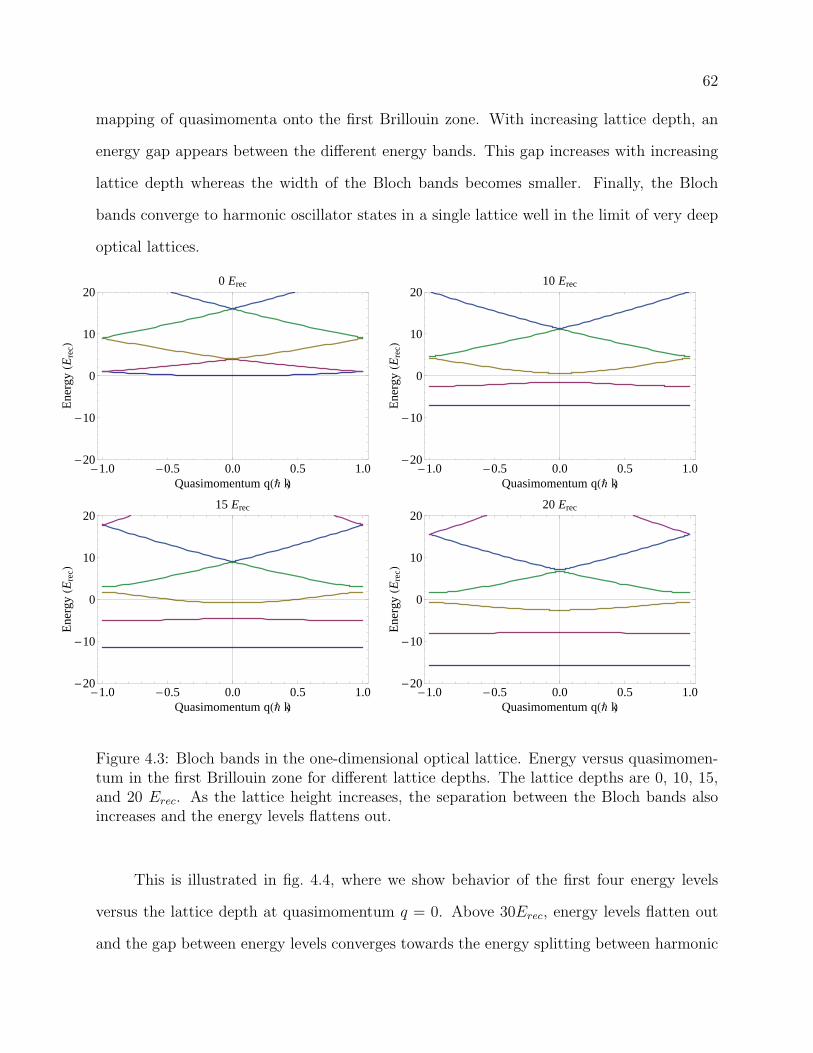
62

mapping of quasimomenta onto the first Brillouin zone. With increasing lattice depth, an

energy gap appears between the different energy bands. This gap increases with increasing

lattice depth whereas the width of the Bloch bands becomes smaller. Finally, the Bloch

bands converge to harmonic oscillator states in a single lattice well in the limit of very deep

optical lattices.

-1.0 -0.5 0.0 0.5 1.0-20

-10

0

10

20

Quasimomentum qHÑ kL

Ene

rgyHE

recL

0 Erec

-1.0 -0.5 0.0 0.5 1.0-20

-10

0

10

20

Quasimomentum qHÑ kL

Ene

rgyHE

recL

10 Erec

-1.0 -0.5 0.0 0.5 1.0-20

-10

0

10

20

Quasimomentum qHÑ kL

Ene

rgyHE

recL

15 Erec

-1.0 -0.5 0.0 0.5 1.0-20

-10

0

10

20

Quasimomentum qHÑ kL

Ene

rgyHE

recL

20 Erec

Figure 4.3: Bloch bands in the one-dimensional optical lattice. Energy versus quasimomen-tum in the first Brillouin zone for different lattice depths. The lattice depths are 0, 10, 15,and 20 Erec. As the lattice height increases, the separation between the Bloch bands alsoincreases and the energy levels flattens out.

This is illustrated in fig. 4.4, where we show behavior of the first four energy levels

versus the lattice depth at quasimomentum q = 0. Above 30Erec, energy levels flatten out

and the gap between energy levels converges towards the energy splitting between harmonic

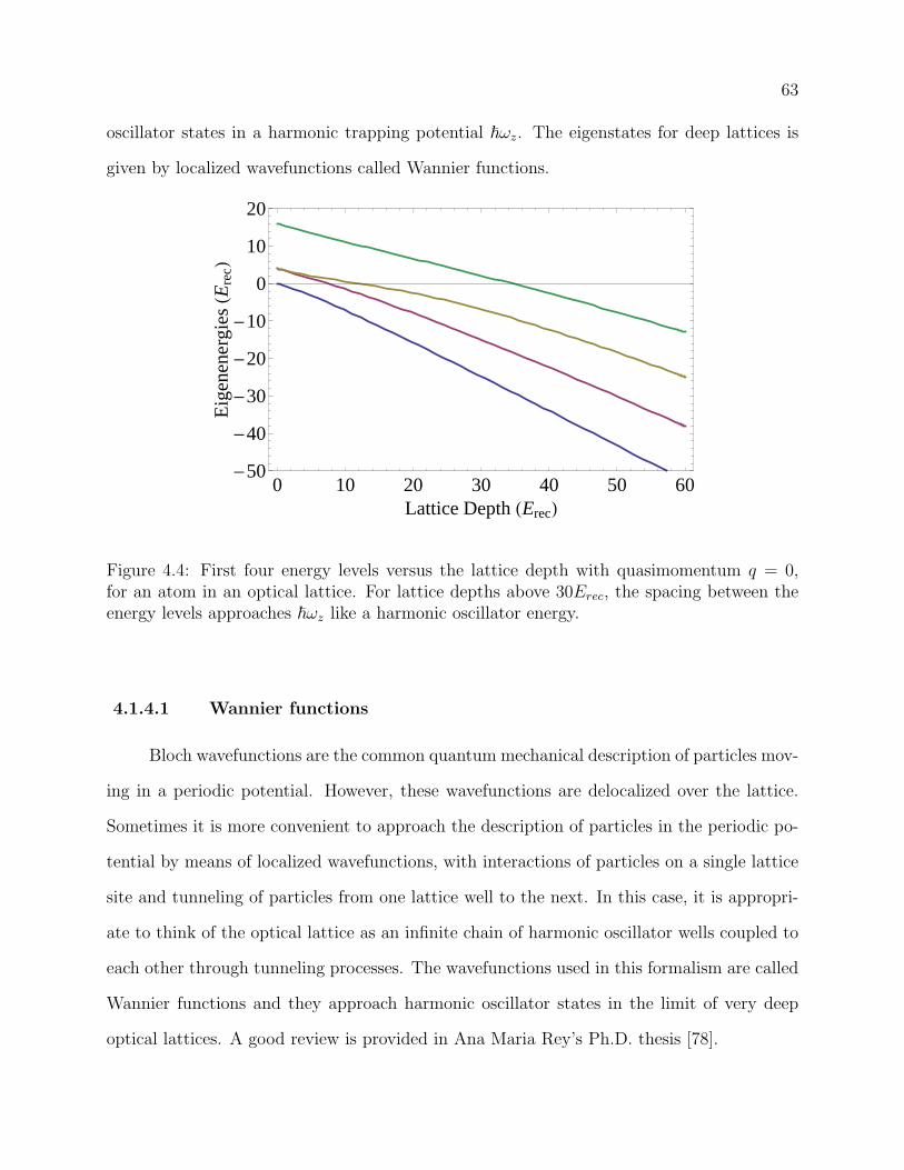
63

oscillator states in a harmonic trapping potential ~ωz. The eigenstates for deep lattices is

given by localized wavefunctions called Wannier functions.

0 10 20 30 40 50 60-50

-40

-30

-20

-10

0

10

20

Lattice Depth HErecL

Eig

enen

ergi

esHE

recL

Figure 4.4: First four energy levels versus the lattice depth with quasimomentum q = 0,for an atom in an optical lattice. For lattice depths above 30Erec, the spacing between theenergy levels approaches ~ωz like a harmonic oscillator energy.

4.1.4.1 Wannier functions

Bloch wavefunctions are the common quantum mechanical description of particles mov-

ing in a periodic potential. However, these wavefunctions are delocalized over the lattice.

Sometimes it is more convenient to approach the description of particles in the periodic po-

tential by means of localized wavefunctions, with interactions of particles on a single lattice

site and tunneling of particles from one lattice well to the next. In this case, it is appropri-

ate to think of the optical lattice as an infinite chain of harmonic oscillator wells coupled to

each other through tunneling processes. The wavefunctions used in this formalism are called

Wannier functions and they approach harmonic oscillator states in the limit of very deep

optical lattices. A good review is provided in Ana Maria Rey’s Ph.D. thesis [78].

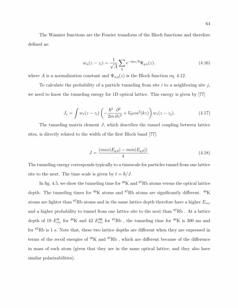
64

The Wannier functions are the Fourier transform of the Bloch functions and therefore

defined as:

wn(z − zi) =1√A

∑q

e−iqzi/~Ψq,n(z). (4.16)

where A is a normalization constant and Ψn,q(z) is the Bloch function eq. 4.12.

To calculate the probability of a particle tunneling from site i to a neighboring site j,

we need to know the tunneling energy for 1D optical lattice. This energy is given by [77]

Jz =

∫w1(z − zi)

(− ~

2

2m

∂2

∂z2+ V0cos

2(kz)

)w1(z − zj). (4.17)

The tunneling matrix element J , which describes the tunnel coupling between lattice

sites, is directly related to the width of the first Bloch band [77]:

J =(max(Eq,0)−min(Eq,0))

4. (4.18)

The tunneling energy corresponds typically to a timescale for particles tunnel from one lattice

site to the next. The time scale is given by t = ~/J .

In fig. 4.5, we show the tunneling time for 40K and 87Rb atoms versus the optical lattice

depth. The tunneling times for 40K atoms and 87Rb atoms are significantly different. 40K

atoms are lighter than 87Rb atoms and in the same lattice depth therefore have a higher Erec

and a higher probability to tunnel from one lattice site to the next than 87Rb . At a lattice

depth of 19 EKrec for 40K and 42 ERb

rec for 87Rb , the tunneling time for 40K is 300 ms and

for 87Rb is 1 s. Note that, these two lattice depths are different when they are expressed in

terms of the recoil energies of 40K and 87Rb , which are different because of the difference

in mass of each atom (given that they are in the same optical lattice, and they also have

similar polarizabilities).

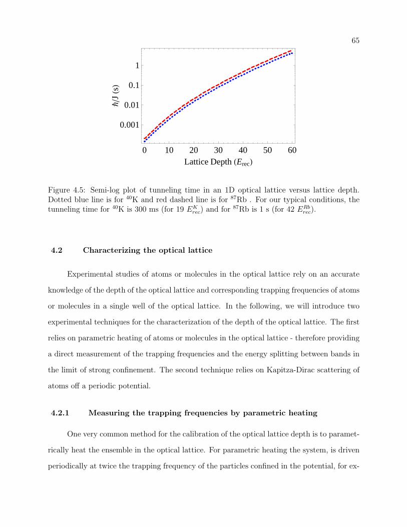
65

0 10 20 30 40 50 60

0.001

0.01

0.1

1

Lattice Depth HErecL

�JHsL

Figure 4.5: Semi-log plot of tunneling time in an 1D optical lattice versus lattice depth.Dotted blue line is for 40K and red dashed line is for 87Rb . For our typical conditions, thetunneling time for 40K is 300 ms (for 19 EK

rec) and for 87Rb is 1 s (for 42 ERbrec).

4.2 Characterizing the optical lattice

Experimental studies of atoms or molecules in the optical lattice rely on an accurate

knowledge of the depth of the optical lattice and corresponding trapping frequencies of atoms

or molecules in a single well of the optical lattice. In the following, we will introduce two

experimental techniques for the characterization of the depth of the optical lattice. The first

relies on parametric heating of atoms or molecules in the optical lattice - therefore providing

a direct measurement of the trapping frequencies and the energy splitting between bands in

the limit of strong confinement. The second technique relies on Kapitza-Dirac scattering of

atoms off a periodic potential.

4.2.1 Measuring the trapping frequencies by parametric heating

One very common method for the calibration of the optical lattice depth is to paramet-

rically heat the ensemble in the optical lattice. For parametric heating the system, is driven

periodically at twice the trapping frequency of the particles confined in the potential, for ex-

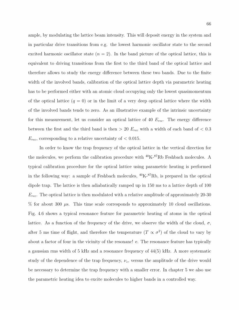
66

ample, by modulating the lattice beam intensity. This will deposit energy in the system and

in particular drive transitions from e.g. the lowest harmonic oscillator state to the second

excited harmonic oscillator state (n = 2). In the band picture of the optical lattice, this is

equivalent to driving transitions from the first to the third band of the optical lattice and

therefore allows to study the energy difference between these two bands. Due to the finite

width of the involved bands, calibration of the optical lattice depth via parametric heating

has to be performed either with an atomic cloud occupying only the lowest quasimomentum

of the optical lattice (q = 0) or in the limit of a very deep optical lattice where the width

of the involved bands tends to zero. As an illustrative example of the intrinsic uncertainty

for this measurement, let us consider an optical lattice of 40 Erec. The energy difference

between the first and the third band is then > 20 Erec with a width of each band of < 0.3

Erec, corresponding to a relative uncertainty of < 0.015.

In order to know the trap frequency of the optical lattice in the vertical direction for

the molecules, we perform the calibration procedure with 40K-87Rb Feshbach molecules. A

typical calibration procedure for the optical lattice using parametric heating is performed

in the following way: a sample of Feshbach molecules, 40K-87Rb, is prepared in the optical

dipole trap. The lattice is then adiabatically ramped up in 150 ms to a lattice depth of 100

Erec. The optical lattice is then modulated with a relative amplitude of approximately 20-30

% for about 300 µs. This time scale corresponds to approximately 10 cloud oscillations.

Fig. 4.6 shows a typical resonance feature for parametric heating of atoms in the optical

lattice. As a function of the frequency of the drive, we observe the width of the cloud, σ,

after 5 ms time of flight, and therefore the temperature (T ∝ σ2) of the cloud to vary by

about a factor of four in the vicinity of the resonanc! e. The resonance feature has typically

a gaussian rms width of 5 kHz and a resonance frequency of 44(5) kHz. A more systematic

study of the dependence of the trap frequency, νz, versus the amplitude of the drive would

be necessary to determine the trap frequency with a smaller error. In chapter 5 we also use

the parametric heating idea to excite molecules to higher bands in a controlled way.

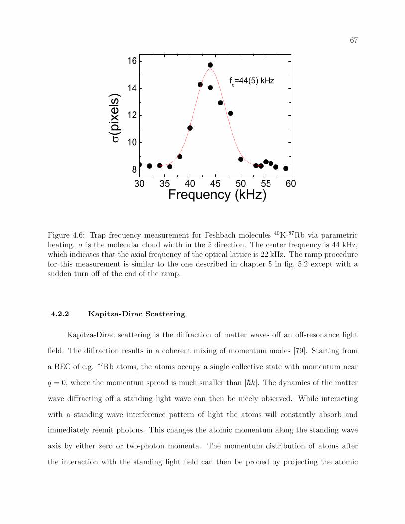
67

30 35 40 45 50 55 608

10

12

14

16

(pix

els)

Frequency (kHz)

fc=44(5) kHz

Figure 4.6: Trap frequency measurement for Feshbach molecules 40K-87Rb via parametricheating. σ is the molecular cloud width in the z direction. The center frequency is 44 kHz,which indicates that the axial frequency of the optical lattice is 22 kHz. The ramp procedurefor this measurement is similar to the one described in chapter 5 in fig. 5.2 except with asudden turn off of the end of the ramp.

4.2.2 Kapitza-Dirac Scattering

Kapitza-Dirac scattering is the diffraction of matter waves off an off-resonance light

field. The diffraction results in a coherent mixing of momentum modes [79]. Starting from

a BEC of e.g. 87Rb atoms, the atoms occupy a single collective state with momentum near

q = 0, where the momentum spread is much smaller than |~k|. The dynamics of the matter

wave diffracting off a standing light wave can then be nicely observed. While interacting

with a standing wave interference pattern of light the atoms will constantly absorb and

immediately reemit photons. This changes the atomic momentum along the standing wave

axis by either zero or two-photon momenta. The momentum distribution of atoms after

the interaction with the standing light field can then be probed by projecting the atomic

68

quasimomentum onto free space momentum in time of flight expansion.

As a particular case of Kapitza-Dirac scattering, we operate in the Raman-Nath regime

where the atom motion during the interaction with the light field can be neglected. The

population of the diffracted states then only depends on the area of the applied pulse [79],

i.e., ωτ ¿ 1, where τ is the pulse duration and ω is the harmonic oscillator frequency. In

our experiment, τ is on the order of tens of µs and ω = 2π × 28 kHz.

In our experiment, we use Kapitza-Dirac scattering of a 87Rb BEC for an accurate

determination of the depth of the optical lattice. The number of atoms , Pn, in the nth

diffraction order observed in momentum space as a function of interaction time τ is given

by a Bessel function of the first kind Jn [79]:

Pn = J2n(

V0τ

2~). (4.19)

where, V0 is the lattice depth. The dynamics of the atomic population during the pulse in

different diffraction orders then gives accurate information on the optical lattice depth.

Fig. 4.7 shows the experimental procedure for measuring the depth of an optical lattice

by means of matter wave diffraction. First, a BEC is prepared in an optical dipole trap.

The optical dipole trap is then suddenly turned off and at the same time the optical lattice

is flashed on for a variable amount of time τ - typically on the order of tens of µs. Fig. 4.8

shows the dynamics of the diffraction pattern of a 87Rb BEC matter-waves versus the hold

time in the lattice. From these images we extract the fractional amplitudes of different ~k

momentum diffraction order and fit the data to a numerical solution of eq. 4.11 following

reference [79]. Here, only the trap depth is a free parameter. In the particular example, we

extract a depth of 42 Erec.

The discrepancy for the optical lattice’s trap frequency determined via parametric

heating and via Kapitza-Dirac scattering is 15%, where the fist is smaller than the second.

For Kapitza-Dirac scattering with 87Rb , we know the frequency of the optical lattice for 87Rb

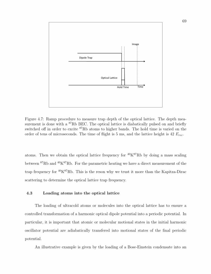
69

Time

Dipole Trap

Optical Lattice

Hold Time

Image

Figure 4.7: Ramp procedure to measure trap depth of the optical lattice. The depth mea-surement is done with a 87Rb BEC. The optical lattice is diabatically pulsed on and brieflyswitched off in order to excite 87Rb atoms to higher bands. The hold time is varied on theorder of tens of microseconds. The time of flight is 5 ms, and the lattice height is 42 Erec.

atoms. Then we obtain the optical lattice frequency for 40K87Rb by doing a mass scaling

between 87Rb and 40K87Rb. For the parametric heating we have a direct measurement of the

trap frequency for 40K87Rb. This is the reson why we trust it more than the Kapitza-Dirac

scattering to determine the optical lattice trap frequency.

4.3 Loading atoms into the optical lattice

The loading of ultracold atoms or molecules into the optical lattice has to ensure a

controlled transformation of a harmonic optical dipole potential into a periodic potential. In

particular, it is important that atomic or molecular motional states in the initial harmonic

oscillator potential are adiabatically transfered into motional states of the final periodic

potential.

An illustrative example is given by the loading of a Bose-Einstein condensate into an

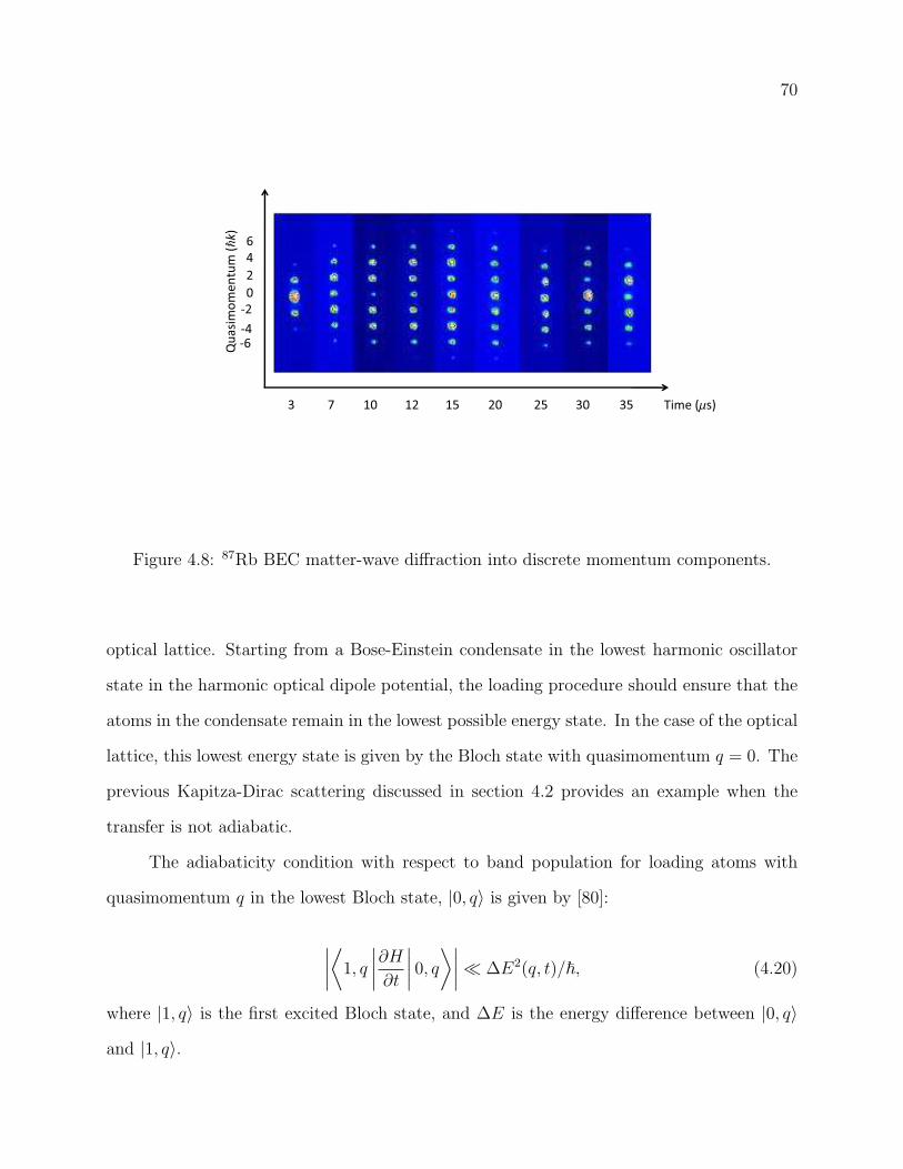
70

73 10 12 15 20 25 30 35 Time ( s)

0

2

-2

4

6

-4-6Q

ua

sim

om

en

tum

(k

)

Figure 4.8: 87Rb BEC matter-wave diffraction into discrete momentum components.

optical lattice. Starting from a Bose-Einstein condensate in the lowest harmonic oscillator

state in the harmonic optical dipole potential, the loading procedure should ensure that the

atoms in the condensate remain in the lowest possible energy state. In the case of the optical

lattice, this lowest energy state is given by the Bloch state with quasimomentum q = 0. The

previous Kapitza-Dirac scattering discussed in section 4.2 provides an example when the

transfer is not adiabatic.

The adiabaticity condition with respect to band population for loading atoms with

quasimomentum q in the lowest Bloch state, |0, q〉 is given by [80]:

∣∣∣∣⟨

1, q

∣∣∣∣∂H

∂t

∣∣∣∣ 0, q

⟩∣∣∣∣ ¿ ∆E2(q, t)/~, (4.20)

where |1, q〉 is the first excited Bloch state, and ∆E is the energy difference between |0, q〉and |1, q〉.

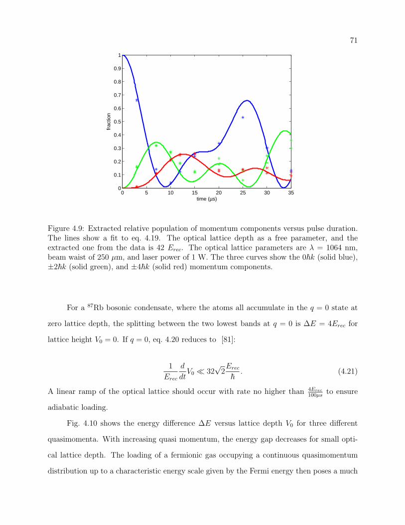
71

0 5 10 15 20 25 30 350

0.1

0.2

0.3

0.4

0.5

0.6

0.7

0.8

0.9

1

time (µs)

frac

tion

Figure 4.9: Extracted relative population of momentum components versus pulse duration.The lines show a fit to eq. 4.19. The optical lattice depth as a free parameter, and theextracted one from the data is 42 Erec. The optical lattice parameters are λ = 1064 nm,beam waist of 250 µm, and laser power of 1 W. The three curves show the 0~k (solid blue),±2~k (solid green), and ±4~k (solid red) momentum components.

For a 87Rb bosonic condensate, where the atoms all accumulate in the q = 0 state at

zero lattice depth, the splitting between the two lowest bands at q = 0 is ∆E = 4Erec for

lattice height V0 = 0. If q = 0, eq. 4.20 reduces to [81]:

1

Erec

d

dtV0 ¿ 32

√2Erec

~. (4.21)

A linear ramp of the optical lattice should occur with rate no higher than 4Erec

100µsto ensure

adiabatic loading.

Fig. 4.10 shows the energy difference ∆E versus lattice depth V0 for three different

quasimomenta. With increasing quasi momentum, the energy gap decreases for small opti-

cal lattice depth. The loading of a fermionic gas occupying a continuous quasimomentum

distribution up to a characteristic energy scale given by the Fermi energy then poses a much

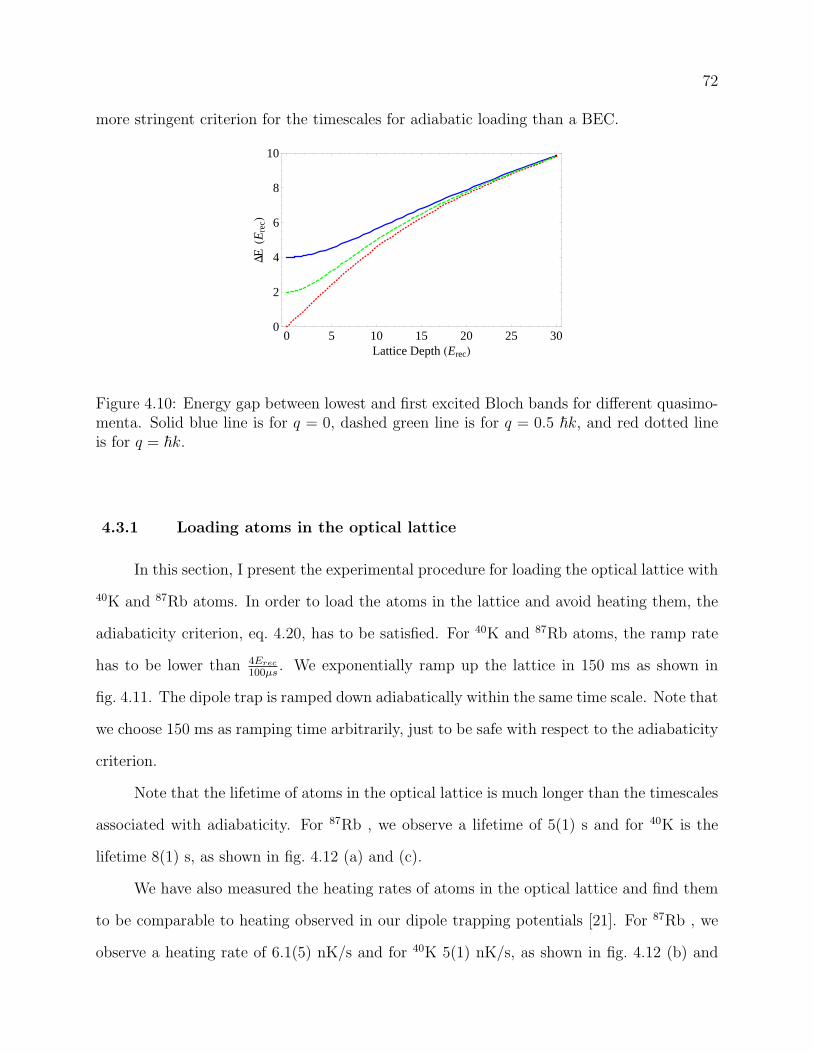
72

more stringent criterion for the timescales for adiabatic loading than a BEC.

0 5 10 15 20 25 300

2

4

6

8

10

Lattice Depth HErecL

DEHE

recL

Figure 4.10: Energy gap between lowest and first excited Bloch bands for different quasimo-menta. Solid blue line is for q = 0, dashed green line is for q = 0.5 ~k, and red dotted lineis for q = ~k.

4.3.1 Loading atoms in the optical lattice

In this section, I present the experimental procedure for loading the optical lattice with

40K and 87Rb atoms. In order to load the atoms in the lattice and avoid heating them, the

adiabaticity criterion, eq. 4.20, has to be satisfied. For 40K and 87Rb atoms, the ramp rate

has to be lower than 4Erec

100µs. We exponentially ramp up the lattice in 150 ms as shown in

fig. 4.11. The dipole trap is ramped down adiabatically within the same time scale. Note that

we choose 150 ms as ramping time arbitrarily, just to be safe with respect to the adiabaticity

criterion.

Note that the lifetime of atoms in the optical lattice is much longer than the timescales

associated with adiabaticity. For 87Rb , we observe a lifetime of 5(1) s and for 40K is the

lifetime 8(1) s, as shown in fig. 4.12 (a) and (c).

We have also measured the heating rates of atoms in the optical lattice and find them

to be comparable to heating observed in our dipole trapping potentials [21]. For 87Rb , we

observe a heating rate of 6.1(5) nK/s and for 40K 5(1) nK/s, as shown in fig. 4.12 (b) and

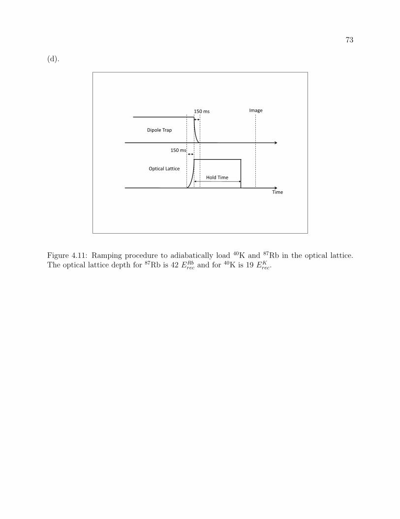
73

(d).

Time

Dipole Trap

Optical Lattice

Hold Time

150 ms Image

150 ms

Figure 4.11: Ramping procedure to adiabatically load 40K and 87Rb in the optical lattice.The optical lattice depth for 87Rb is 42 ERb

rec and for 40K is 19 EKrec.

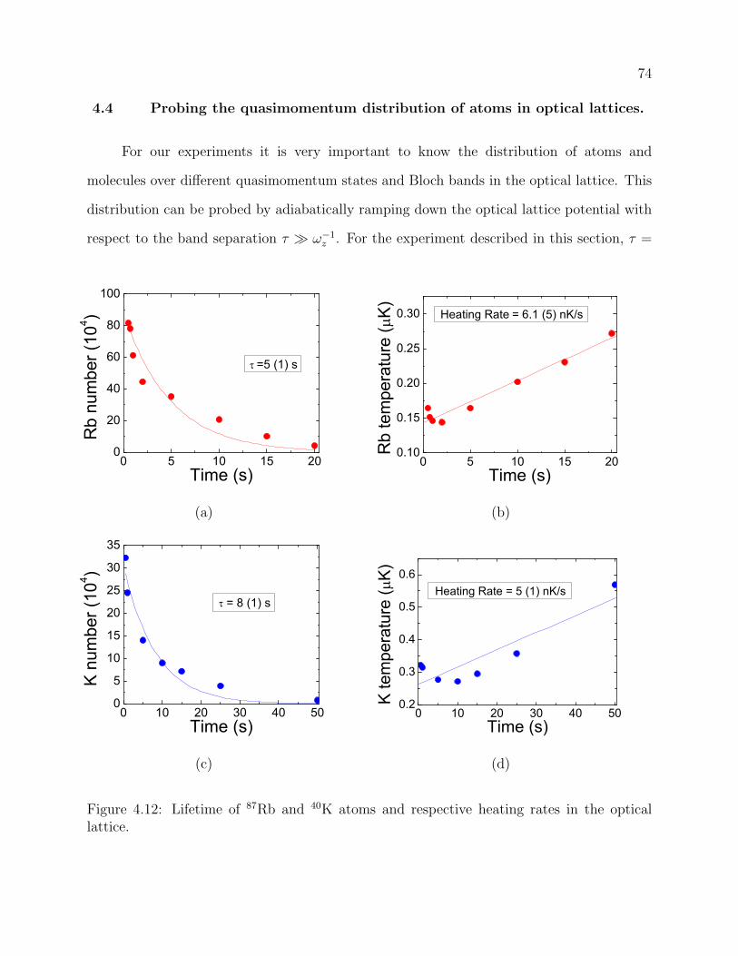
74

4.4 Probing the quasimomentum distribution of atoms in optical lattices.

For our experiments it is very important to know the distribution of atoms and

molecules over different quasimomentum states and Bloch bands in the optical lattice. This

distribution can be probed by adiabatically ramping down the optical lattice potential with

respect to the band separation τ À ω−1z . For the experiment described in this section, τ =

0 5 10 15 200

20

40

60

80

100

=5 (1) s

Rb

num

ber (

104 )

Time (s)0 5 10 15 20

0.10

0.15

0.20

0.25

0.30 Heating Rate = 6.1 (5) nK/s

Rb

tem

pera

ture

(K)

Time (s)

(a) (b)

0 10 20 30 40 500

5

10

15

20

25

30

35

= 8 (1) s

K nu

mbe

r (10

4 )

Time (s)0 10 20 30 40 50

0.2

0.3

0.4

0.5

0.6Heating Rate = 5 (1) nK/s

K te

mpe

ratu

re (

K)

Time (s)

(c) (d)

Figure 4.12: Lifetime of 87Rb and 40K atoms and respective heating rates in the opticallattice.

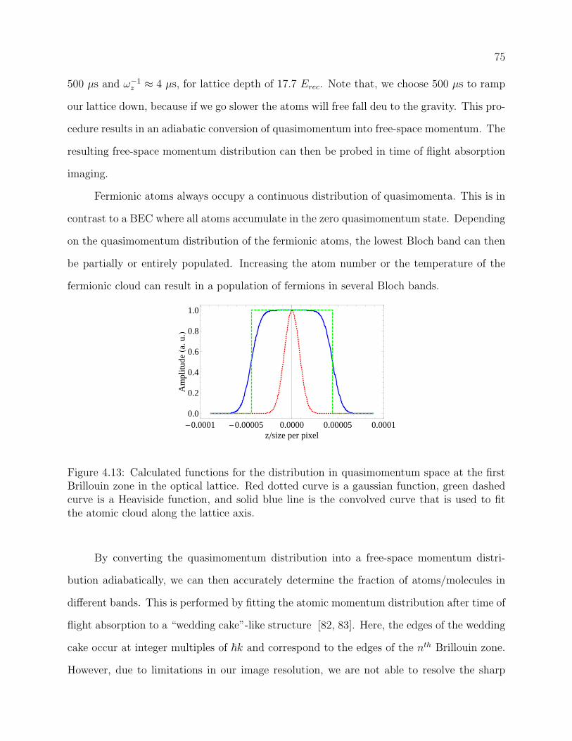
75

500 µs and ω−1z ≈ 4 µs, for lattice depth of 17.7 Erec. Note that, we choose 500 µs to ramp

our lattice down, because if we go slower the atoms will free fall deu to the gravity. This pro-

cedure results in an adiabatic conversion of quasimomentum into free-space momentum. The

resulting free-space momentum distribution can then be probed in time of flight absorption

imaging.

Fermionic atoms always occupy a continuous distribution of quasimomenta. This is in

contrast to a BEC where all atoms accumulate in the zero quasimomentum state. Depending

on the quasimomentum distribution of the fermionic atoms, the lowest Bloch band can then

be partially or entirely populated. Increasing the atom number or the temperature of the

fermionic cloud can result in a population of fermions in several Bloch bands.

-0.0001 -0.00005 0.0000 0.00005 0.00010.0

0.2

0.4

0.6

0.8

1.0

z�size per pixel

Am

plitu

deHa

.u.L

Figure 4.13: Calculated functions for the distribution in quasimomentum space at the firstBrillouin zone in the optical lattice. Red dotted curve is a gaussian function, green dashedcurve is a Heaviside function, and solid blue line is the convolved curve that is used to fitthe atomic cloud along the lattice axis.

By converting the quasimomentum distribution into a free-space momentum distri-

bution adiabatically, we can then accurately determine the fraction of atoms/molecules in

different bands. This is performed by fitting the atomic momentum distribution after time of

flight absorption to a “wedding cake”-like structure [82, 83]. Here, the edges of the wedding

cake occur at integer multiples of ~k and correspond to the edges of the nth Brillouin zone.

However, due to limitations in our image resolution, we are not able to resolve the sharp

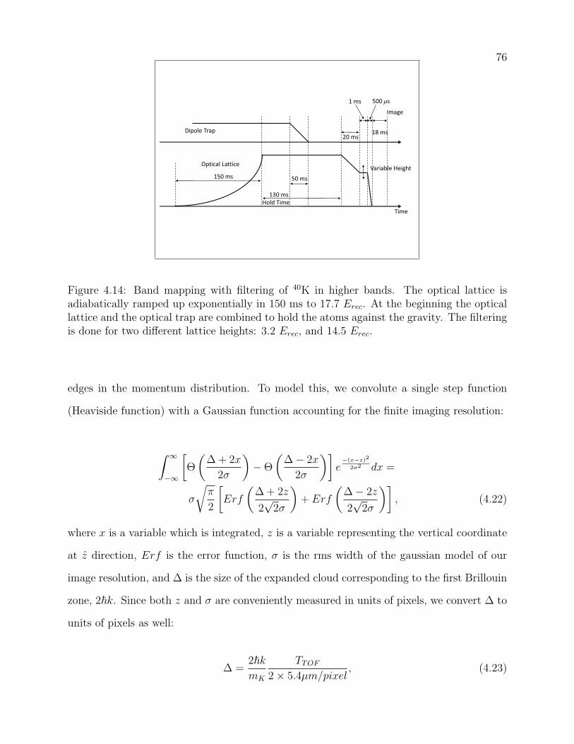
76

Time

Dipole Trap

Optical Lattice

Hold Time

150 ms

1 ms

Image

Variable Height

18 ms20 ms

50 ms

130 ms

500 s

Figure 4.14: Band mapping with filtering of 40K in higher bands. The optical lattice isadiabatically ramped up exponentially in 150 ms to 17.7 Erec. At the beginning the opticallattice and the optical trap are combined to hold the atoms against the gravity. The filteringis done for two different lattice heights: 3.2 Erec, and 14.5 Erec.

edges in the momentum distribution. To model this, we convolute a single step function

(Heaviside function) with a Gaussian function accounting for the finite imaging resolution:

∫ ∞

−∞

[Θ

(∆ + 2x

2σ

)−Θ

(∆− 2x

2σ

)]e−(x−z)2

2σ2 dx =

σ

√π

2

[Erf

(∆ + 2z

2√

2σ

)+ Erf

(∆− 2z

2√

2σ

)], (4.22)

where x is a variable which is integrated, z is a variable representing the vertical coordinate

at z direction, Erf is the error function, σ is the rms width of the gaussian model of our

image resolution, and ∆ is the size of the expanded cloud corresponding to the first Brillouin

zone, 2~k. Since both z and σ are conveniently measured in units of pixels, we convert ∆ to

units of pixels as well:

∆ =2~kmK

TTOF

2× 5.4µm/pixel, (4.23)

77

where TTOF = 18 ms is the time of flight, mK is the atomic mass of 40K , σ is the image

resolution in pixels, and 5.4 µm/pixel is the conversion from micrometers to pixels at the

image. The factor of 2 multiplying the 5.4 µm/pixel is because of the binning of the image

was 2. Fig. 4.13 shows the Heaviside (dashed green), the Gaussian (dotted red) and the

resulting convoluted (solid blue) functions.

We multiply the result of eq. 4.22 by A/2 where A is an amplitude scaling factor, and

also by shifting the center of the function by zc. We replace the amplitude because we want

to extract the relative atom (molecule) population in the lattice levels. We then fit the data

with three free parameters: the amplitude A, the image resolution σ, and the center zc (zc

is also in units of camera pixels). The fitting function for atomic distribution in the first

Brillouin zone is given by:

f(z) = A/2

[Erf

(∆ + 2(z − zc)

2√

2σ

)+ Erf

(∆− 2(z − zc)

2√

2σ

)], (4.24)

and the fitting function for a distribution in both first and second Brillouin zones is given

by:

f(z) = A/2

[Erf

(∆ + 2(z − zc)

2√

2σ

)+ Erf

(∆− 2(z − zc)

2√

2σ

)]

+B/2

[Erf

(−∆ + 2(z − zc)

2√

2σ

)+ Erf

(−∆− 2(z − zc)

2√

2σ

)]

+B/2

[Erf

(2∆ + 2(z − zc)

2√

2σ

)+ Erf

(2∆− 2(z − zc)

2√

2σ

)]. (4.25)

where B is the amplitude of the distribution in the second Brillouin zone.

Fig. 4.15 shows two illustrative examples how we extract the band population using

the procedure described above. In fig. 4.15(a), all 40K atoms have been loaded into the

lowest Bloch band only and we therefore observe a single sharp momentum distribution

in the vertical direction with the largest momentum given by ~k. Fig. 4.15(b) shows the

corresponding radially integrated momentum distribution of 40K atoms in the first Brillouin

78

zone. Although the edges of the momentum distribution are blurred due to the finite imaging

resolution, it can clearly be seen that all atoms occupy momentum states within the first

Brillouin zone.

Heating the atomic 40K ensembles to temperatures in the 400 nK range, atoms will not

only occupy the first but also the second Brillouin zone. This is shown in fig. 4.15(c) and (d).

Now, atoms also occupy quasimomenta −2~k < q < 2~k and we can extract the fraction of

atoms in higher bands by fitting eq. 4.25 to the wedding cake structure and comparing the

two areas underneath the fitting curve. From this, we determine the fraction of 40K atoms

in the second Brillouin zone to be approximately 28%.

It is known that collisions between atoms in higher bands and atoms in the lowest

band induce very fast collisional loss in the sample, due to a two-body decay process [84].

To circumvent this issue and ensure the preparation of atoms in the lowest Bloch band only,

we introduce a filtering procedure during the optical lattice loading. The filtering will result

in fast tunneling of atoms in higher optical bands out of the optical lattice. Atoms in the

lowest Bloch band will stay in the lattice. Our ramping procedure is shown in fig. 4.14,

where the optical lattice is adiabatically ramped up in 150 ms to the height of 17.7 Erec.

The atoms are held in the lattice for 130 ms and the dipole trap is adiabatically ramped

down in 50 ms. The filtering is accomplished by ramping down the lattice in 20 ms holding

it for 1 ms and then ramped down in 500 µs to 0 Erec, for the band mapping. In fig. 4.15a

and b, I show the 40K atoms all in the first Brillouin zone due to the filtering procedure. In

order to filter atoms in the second band, the optical lattice height was reduced to 3.2 Erec.

In fig. 4.15c and d, I show the 40K atoms in the first and second Brillouin zones. The optical

lattice height was reduced to 14.5 Erec. The filtering procedure was not used for molecules

in the optical lattice.

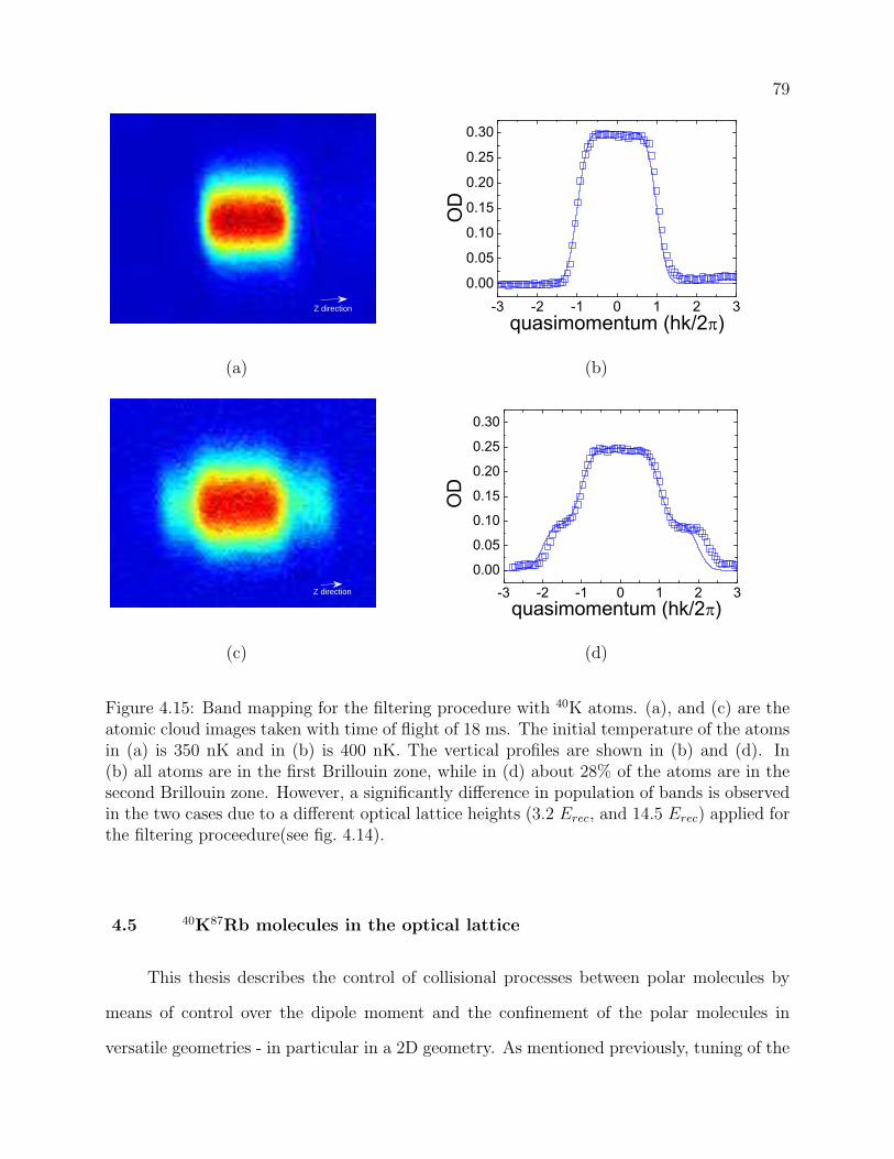
79

Z direction -3 -2 -1 0 1 2 30.00

0.05

0.10

0.15

0.20

0.25

0.30

OD

quasimomentum (hk/2 )

(a) (b)

Z direction -3 -2 -1 0 1 2 30.00

0.05

0.10

0.15

0.20

0.25

0.30

OD

quasimomentum (hk/2 )

(c) (d)

Figure 4.15: Band mapping for the filtering procedure with 40K atoms. (a), and (c) are theatomic cloud images taken with time of flight of 18 ms. The initial temperature of the atomsin (a) is 350 nK and in (b) is 400 nK. The vertical profiles are shown in (b) and (d). In(b) all atoms are in the first Brillouin zone, while in (d) about 28% of the atoms are in thesecond Brillouin zone. However, a significantly difference in population of bands is observedin the two cases due to a different optical lattice heights (3.2 Erec, and 14.5 Erec) applied forthe filtering proceedure(see fig. 4.14).

4.5 40K87Rb molecules in the optical lattice

This thesis describes the control of collisional processes between polar molecules by

means of control over the dipole moment and the confinement of the polar molecules in

versatile geometries - in particular in a 2D geometry. As mentioned previously, tuning of the

80

trapping geometry from 3D to 2D is achieved in the experiment by gradually increasing the

depth of an optical lattice and transferring molecules from a dipole trap to a 1D lattice.

In this section, we will describe how we prepare molecules in the lowest band of the

optical lattice and how we control the population in different bands. Polar molecules are

formed in the lattice following the ideas already outlined in chapter 2 and earlier sections

of chapter 4. In the first step, we load atoms from the optical dipole trap into the optical

lattice as described above. The optical lattice is ramped up adiabatically in 150 ms following

a exponential ramp, then the dipole trap is ramped down within 150 ms. In the next step,

we prepare Feshbach molecules in the optical lattice by ramping an external magnetic field

through a Fano-Feshbach resonance. We subsequently transfer the Feshbach molecules to

the rotational and vibrational ground state using STIRAP.

After preparing molecules in the optical lattice, we measure their heating rate. The

result is shown in fig. 4.17. We observe a heating rate of 105(12) nK/s. The origin of this

heating, which is an order of magnitude larger than what we measure for atoms is unknown.

We speculate that extra heating might be induced by imperfections in the potential, forma-

tion of molecules in higher bands, anti-evaporation induced by number loss or non-adiabatic

heating due to a sudden change of the external trapping potential.

For our experiments, we need a maximum number of molecules in the lowest band of the

optical lattice. In order to optimize this number, we have experimentally compared different

procedures for forming molecules in the optical lattice. The first procedure is to prepare

molecules in the optical dipole trap first and then in a subsequent step load these molecules

into the optical lattice as shown in fig. 4.18. To evaluate this procedure, we measured the

number of molecules in the optical lattice versus the lattice depth. However, we observed a

very fast loss after loading the molecules into the lattice. Presumably, this loss of molecules

was due to a large fraction of the molecules accumulating in other than the lowest band of

the optical lattice and fast s-wave two-body losses [84].

In the second experiment, we load atoms in the optical lattice and then convert atoms

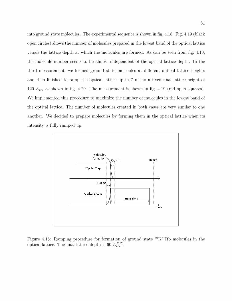
81

into ground state molecules. The experimental sequence is shown in fig. 4.18. Fig. 4.19 (black

open circles) shows the number of molecules prepared in the lowest band of the optical lattice

versus the lattice depth at which the molecules are formed. As can be seen from fig. 4.19,

the molecule number seems to be almost independent of the optical lattice depth. In the

third measurement, we formed ground state molecules at different optical lattice heights

and then finished to ramp the optical lattice up in 7 ms to a fixed final lattice height of

120 Erec as shown in fig. 4.20. The measurement is shown in fig. 4.19 (red open squares).

We implemented this procedure to maximize the number of molecules in the lowest band of

the optical lattice. The number of molecules created in both cases are very similar to one

another. We decided to prepare molecules by forming them in the optical lattice when its

intensity is fully ramped up.

� �������������� ��� ���� �� ����� ��

��� �� �������� ��

����� ���!���"��#

Figure 4.16: Ramping procedure for formation of ground state 40K87Rb molecules in theoptical lattice. The final lattice depth is 60 EKRb

rec .

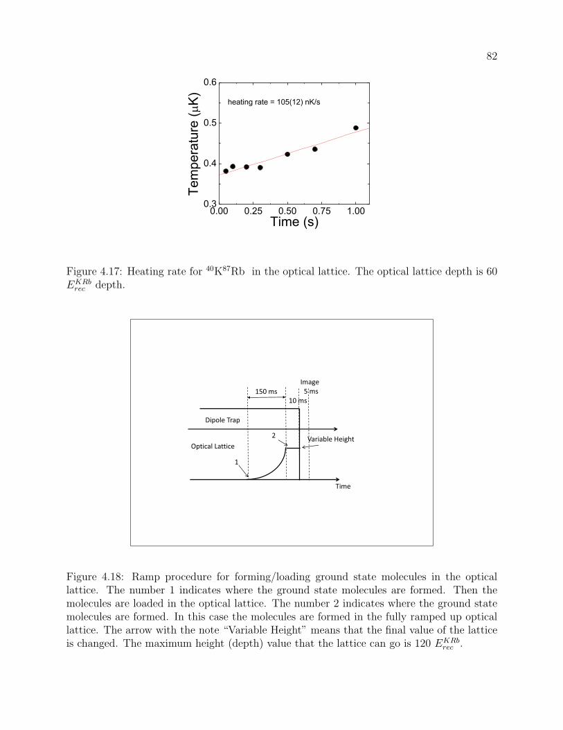
82

0.00 0.25 0.50 0.75 1.000.3

0.4

0.5

0.6

Tem

pera

ture

(K)

Time (s)

heating rate = 105(12) nK/s

Figure 4.17: Heating rate for 40K87Rb in the optical lattice. The optical lattice depth is 60EKRb

rec depth.

Dipole Trap

Image

150 ms

Time

Optical Lattice

1

2Variable Height

10 ms

5 ms

Figure 4.18: Ramp procedure for forming/loading ground state molecules in the opticallattice. The number 1 indicates where the ground state molecules are formed. Then themolecules are loaded in the optical lattice. The number 2 indicates where the ground statemolecules are formed. In this case the molecules are formed in the fully ramped up opticallattice. The arrow with the note “Variable Height” means that the final value of the latticeis changed. The maximum height (depth) value that the lattice can go is 120 EKRb

rec .

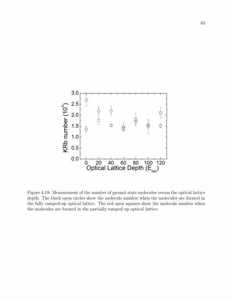
83

0 20 40 60 80 100 1200.0

0.5

1.0

1.5

2.0

2.5

3.0

KRb

num

ber (

104 )

Optical Lattice Depth (Erec)

Figure 4.19: Measurement of the number of ground state molecules versus the optical latticedepth. The black open circles show the molecule number when the molecules are formed inthe fully ramped-up optical lattice. The red open squares show the molecule number whenthe molecules are formed in the partially ramped up optical lattice.

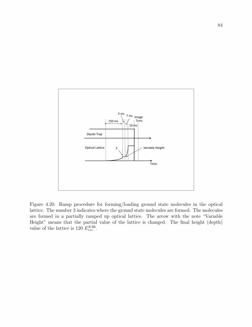
84

Dipole Trap

Image

150 ms

Time

Optical Lattice Variable Height3

3 ms7 ms

10 ms

5 ms

Figure 4.20: Ramp procedure for forming/loading ground state molecules in the opticallattice. The number 3 indicates where the ground state molecules are formed. The moleculesare formed in a partially ramped up optical lattice. The arrow with the note “VariableHeight” means that the partial value of the lattice is changed. The final height (depth)value of the lattice is 120 EKRb

rec .

Chapter 5

Suppression of Inelastic Collisions in 2D geometry

As we have shown in chapter 3, atom-exchange chemical reactions dominate the colli-

sional dynamics in the ultracold molecular gas when the gas is confined in three dimensions

(3D). The inelastic rate increases with increasing dipole moment and leads to a very fast loss

of molecules from the gas and strong heating [40]. The inelastic loss processes dominate over

elastic collisional processes, thereby preventing evaporative cooling of the molecular sample

into quantum degeneracy. However, the chemical reactions are dominated by “head-to-tail”

collisions between polar molecules where the attractive interactions between the dipoles sig-

nificantly reduces the height of the p-wave collisional barrier. “Side-by-side” collisions should

however be suppressed with increasing dipole moment. In this chapter, I report the suppres-

sion of inelastic “head-to-tail” collisions in the molecular sample by confining the molecules

in a 2D geometry. This suppression of inelastic collisions by about 2 orders of magnitudes as

compared to that in a 3D geometry promises to open the way towards evaporative cooling

of polar molecules into quantum degeneracy.

In the following, I will discuss how attractive “head-to-tail” collisions can be controlled

and suppressed by means of 2D spatial confinement. I will define the concept of stereodynam-

ics and explain how the quantum statistics and the quasi-two-dimensional confinement come

together to exclude certain collisional decay channels. I will then discuss our experiments

with polar molecules in a 2D geometry. I will explore collisions between polar molecules

in distinguishable and indistinguishable quantum states of motion and in particular discuss

86

the suppression of chemical reactions for 40K87Rb molecules confined in the optical lattice.

Throughout this chapter, I closely follow reference [74], which describe our work.

5.1 Chemical Reaction Rates and Stereodynamics

Chemical reaction rates often depend strongly on stereodynamics, namely the orienta-

tion and tranlational movement of molecules in three-dimensional space [85, 86, 87]. An ultra-

cold molecular gas, with a temperature below 1 µK, provides an unusual regime for chemistry,

where polar molecules can be oriented using an external electric field and where, moreover,

the motion of two colliding molecules is strictly quantized. As explained in chapter 3, atom-

exchange reactions were observed in a trapped ultracold gas of 40K87Rb molecules [39]. In an

external electric field, these exothermic and barrierless bimolecular reactions, KRb+KRb→K2+Rb2, occur at a rate that rises steeply with increasing dipole moment to the power of

six [40]. The quantum stereodynamics of the ultracold collisions can be used to suppress the

chemical reaction rate by nearly two orders of magnitude [74]. We use an optical lattice to

confine fermionic polar molecules in a quasi-two-dimensional, pancake-like geometry, with

the dipoles oriented along the tight confinement direction [33, 88], perpendicular to each

pancake. With the combination of sufficiently tight confinement and Fermi statistics of the

molecules, two polar molecules can approach each other only in a “side-by-side” collision,

where the chemical reaction rate is suppressed by the repulsive dipole-dipole interaction.

The suppression of the reaction rate requires quantum-state control of both the internal and

external degrees of freedom of the molecules.

Two colliding polar molecules interact via long-range dipole-dipole forces well before

they reach the shorter distance scales where chemical forces become relevant. Therefore, the

spatial anisotropy of the dipolar interaction can play an essential role in the stereochemistry

of bimolecular reactions of polar molecules. In general, one expects the attraction between

oriented dipoles in a “head-to-tail” collision to be favorable for chemical reactions, while

the repulsion between two oriented polar molecules in a “side-by-side” collision presents an

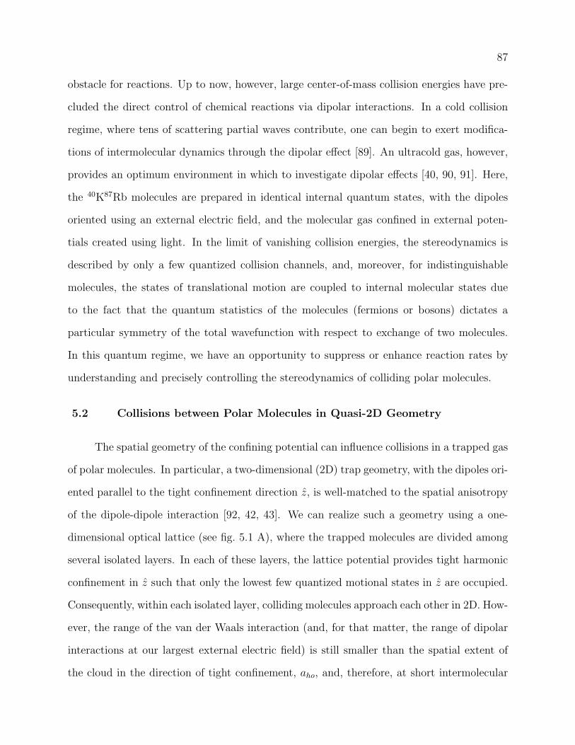
87

obstacle for reactions. Up to now, however, large center-of-mass collision energies have pre-

cluded the direct control of chemical reactions via dipolar interactions. In a cold collision

regime, where tens of scattering partial waves contribute, one can begin to exert modifica-

tions of intermolecular dynamics through the dipolar effect [89]. An ultracold gas, however,

provides an optimum environment in which to investigate dipolar effects [40, 90, 91]. Here,

the 40K87Rb molecules are prepared in identical internal quantum states, with the dipoles

oriented using an external electric field, and the molecular gas confined in external poten-

tials created using light. In the limit of vanishing collision energies, the stereodynamics is

described by only a few quantized collision channels, and, moreover, for indistinguishable

molecules, the states of translational motion are coupled to internal molecular states due

to the fact that the quantum statistics of the molecules (fermions or bosons) dictates a

particular symmetry of the total wavefunction with respect to exchange of two molecules.

In this quantum regime, we have an opportunity to suppress or enhance reaction rates by

understanding and precisely controlling the stereodynamics of colliding polar molecules.

5.2 Collisions between Polar Molecules in Quasi-2D Geometry

The spatial geometry of the confining potential can influence collisions in a trapped gas

of polar molecules. In particular, a two-dimensional (2D) trap geometry, with the dipoles ori-

ented parallel to the tight confinement direction z, is well-matched to the spatial anisotropy

of the dipole-dipole interaction [92, 42, 43]. We can realize such a geometry using a one-

dimensional optical lattice (see fig. 5.1 A), where the trapped molecules are divided among

several isolated layers. In each of these layers, the lattice potential provides tight harmonic

confinement in z such that only the lowest few quantized motional states in z are occupied.

Consequently, within each isolated layer, colliding molecules approach each other in 2D. How-

ever, the range of the van der Waals interaction (and, for that matter, the range of dipolar

interactions at our largest external electric field) is still smaller than the spatial extent of

the cloud in the direction of tight confinement, aho, and, therefore, at short intermolecular

88

distances a collision still must be treated in three dimensions (3D).

We now consider the quantized collision channels that define the stereodynamics in

this quasi-2D geometry. For intermolecular separations that are much larger than aho, the

relative motion of the two molecules is described by a quantized angular momentum, ~M ,

around the z axis, as well as by a quantized relative motion along z. As discussed above, the

stereodynamics of ultracold collisions of indistinguishable molecules is strongly influenced

by the fact that the two-molecule wavefunction must obey an overall symmetry with respect

to the exchange of the identical molecules. Following the formalism from reference [93], as

molecules are identical, a overall wavefunction Ψ is constructed in a way that the molecular

permutation operator P gives:

PΨ = εP Ψ, (5.1)

where εP = 1 for bosonic molecules and εP = −1 for fermionic molecules. The overall

wavefunction Ψ, has an internal wavefunction |α1α2, η〉, where α1 and α2 represent the

electronic, vibrational, rotational and nuclear spin degrees of freedom of molecules 1 and

2, and the external wavefunction representing the confinement in one dimension, i.e., the

confinement in the plane perpendicular to the z direction, due to the optical lattice. The

symmetrized states of the external wavefunction are given by:

|n1n2, γ〉 =1√

2(1 + δn1,n2)[|n1n2〉+ γ |n2n1〉] , (5.2)

where n1 and n2 are the harmonic oscillator states for molecules 1 and 2. For molecules in

identical harmonic oscillator states n1 = n2, γ = 1, δn1,n2 = 1; for molecules in different

states n1 6= n2, δn1,n2 = 0, and P |n1n2, γ〉 = γ |n1n2, γ〉. An essential aspect of relative

motion in the plane perpendicular to the z direction is the exchange symmetry of this part

of the two-molecule wavefunction, which we identify with a quantum number γ. For the

symmetric case, γ = 1 and for the antisymmetric case, γ = −1. For two molecules in the

same z harmonic oscillator state, γ = 1; while both γ = 1 and γ = −1 are possible for

two molecules in different harmonic oscillator states. For the internal wavefunction, the

89

symmetrized states are given by:

|α1α2, η〉 =1√

2(1 + δα1,α2)[|α1α2〉+ η |α2α1〉] , (5.3)

where for molecules in the same internal states α1 = α2, δα1,α2 = 1, for molecules in different

internal states α1 6= α2, δα1,α2 = 0. Similarly, we use a quantum number η to keep track

of the exchange symmetry of the part of the wavefunction that describes the internal states

of the two molecules. For two molecules in the same internal quantum state, η = 1, while

η = ±1 for molecules in different internal states.

In 2D, these three quantum numbers (M, γ, η) are sufficient to describe the quantum

stereodynamics. However, because the interactions at short range must be described in

3D, the quantum number corresponding to the 3D angular momentum, L, as well as M ,

becomes relevant. With collisional channels described by quantum numbers η, L, γ, and M ,

the fermionic symmetry can be concisely stated in the following relations [93]:

η(−1)L = −1, Short range, 3D (5.4)

ηγ(−1)M = −1. Long range, 2D (5.5)

For ultracold collisions where long range interactions play decisive roles, the chemical

reaction rate will be dominated by the allowed collision channel with the lowest centrifugal

barrier. Combining this fact with the relations above, we identify three collision channels

relevant to the stereodynamics, and we label these |1〉, |2〉, and |3〉, in order of increasing

centrifugal barrier heights. The dipole-dipole interaction mixes states with different L. How-

ever, for convenience, we will refer to the lowest energy adiabatic channel, which does not

have a centrifugal barrier, as L = 0. Similarly, we will use L = 1 to denote the odd-L adia-

batic channel with the lowest centrifugal barrier. Collision channel |1〉 has η = −1, L = 0,

γ = 1, and M = 0, and corresponds to spatially isotropic collisions. Collision channel |2〉 has

η = 1, L = 1, γ = −1, and M = 0, and is the quantum analog of “head-to-tail” collisions.

Collision channel |3〉 has η = 1, L = 1, γ = 1, and M = ±1, and is the quantum analog of

90

“side-by-side” collisions. Fig. 5.1 B shows schematically the adiabatic potentials for these

three lowest energy collision channels. Channels |1〉 and |2〉 become increasingly favorable

for chemical reactions as the dipole-dipole interaction strength is increased, for example by

increasing the external electric field−→E . In contrast, channel |3〉 has a centrifugal barrier

whose height increases for higher dipole moment, within the |−→E | range considered in this

work. This barrier hence continues to prevent molecules from reaching short range.

Fig. 5.1 C shows how these different collision channels can be accessed through control

of the internal molecular states and the z motional states. In fig. 5.1 C, molecules in different

internal states are shown in different colors and the harmonic oscillator states in z are

labeled by v. In case (1), for two molecules in different internal molecular states and in

any combination of v levels, channel |1〉 is allowed when η = −1, resulting in no centrifugal

barrier. In case (2), when the molecules are prepared in identical internal molecular states

but in different v levels, the lowest energy collision channel is |2〉 (“head-to-tail”), which is

allowed when γ = −1. In case (3), where the molecules are prepared in the same internal

state and the same v level, the two lower energy collision channels are no longer allowed,

and reactions can only proceed through channel |3〉 (“side-by-side”). This case is the least

favorable for chemical reactions.

5.3 Band Mapping of Molecules

We create a trapped, ultracold gas of 40K87Rb molecules, in their lowest energy ro-

vibrational level and in a single hyperfine state. To confine the molecules, we start with

a crossed-beam optical dipole trap, with a harmonic trapping frequency of 180 Hz along

the vertical direction (z) and 25 Hz in the transverse directions. We ramp up the optical

lattice along z in 150 ms as shown in fig. 5.2. Both dipolar trap and optical lattice beams

are linearly polarized and their polarizations are mutually orthogonal. The structure of the

optical lattice is like a “stack of pancakes”. Each pancake (layer) of the optical lattice is

tightly confining in z with a harmonic trapping frequency of νz = 23 kHz for the molecules;

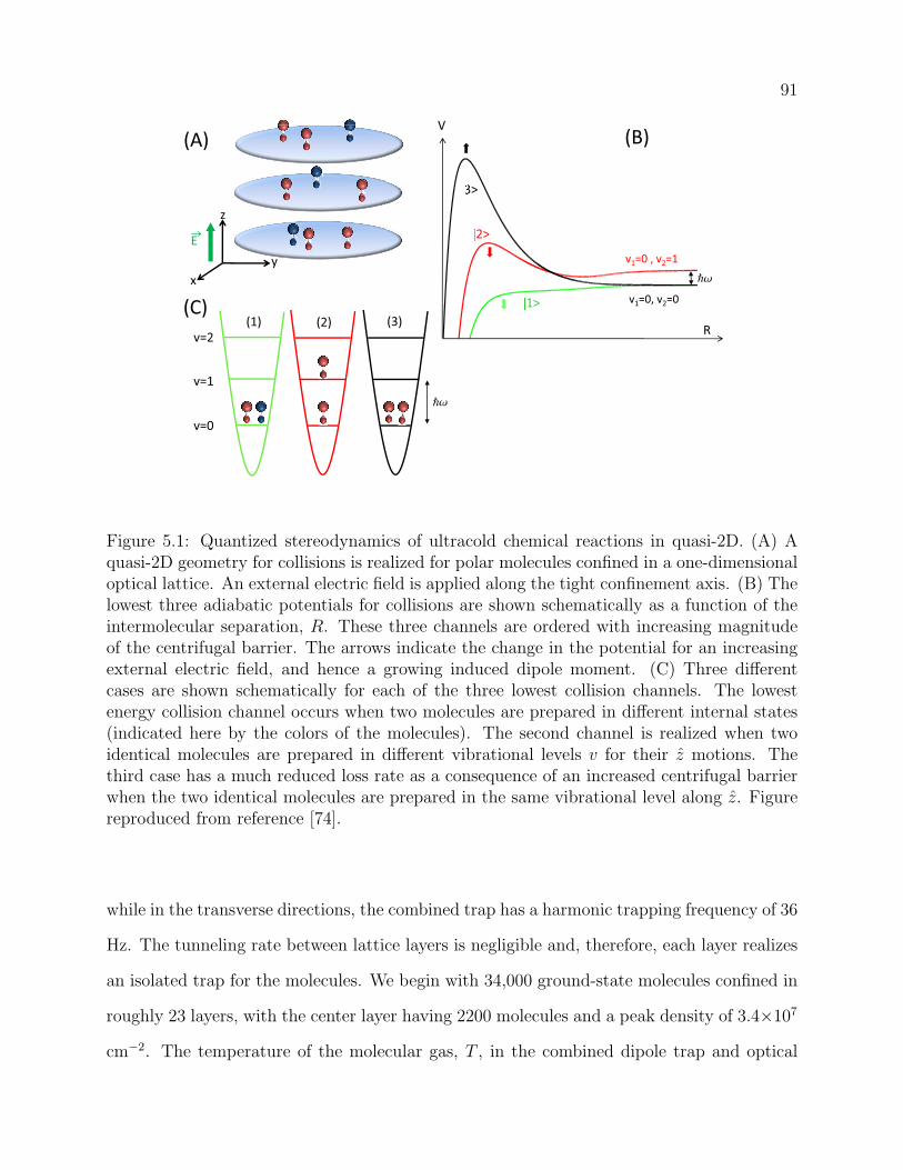
91

v1=0, v2=0

v1=0 , v2=1

1>

2>

3>

(B)

R

V

(A)

(C)

v=2

v=1

v=0

(3)

x

y

z

E

(2)(1)

Figure 5.1: Quantized stereodynamics of ultracold chemical reactions in quasi-2D. (A) Aquasi-2D geometry for collisions is realized for polar molecules confined in a one-dimensionaloptical lattice. An external electric field is applied along the tight confinement axis. (B) Thelowest three adiabatic potentials for collisions are shown schematically as a function of theintermolecular separation, R. These three channels are ordered with increasing magnitudeof the centrifugal barrier. The arrows indicate the change in the potential for an increasingexternal electric field, and hence a growing induced dipole moment. (C) Three differentcases are shown schematically for each of the three lowest collision channels. The lowestenergy collision channel occurs when two molecules are prepared in different internal states(indicated here by the colors of the molecules). The second channel is realized when twoidentical molecules are prepared in different vibrational levels v for their z motions. Thethird case has a much reduced loss rate as a consequence of an increased centrifugal barrierwhen the two identical molecules are prepared in the same vibrational level along z. Figurereproduced from reference [74].

while in the transverse directions, the combined trap has a harmonic trapping frequency of 36

Hz. The tunneling rate between lattice layers is negligible and, therefore, each layer realizes

an isolated trap for the molecules. We begin with 34,000 ground-state molecules confined in

roughly 23 layers, with the center layer having 2200 molecules and a peak density of 3.4×107

cm−2. The temperature of the molecular gas, T , in the combined dipole trap and optical

92

lattice can be varied between 500 nK and 800 nK by changing the initial atom gas conditions.

To completely freeze out motion of the molecules along z requires that kBT ¿ hνz, where

kB is Boltzmann’s constant. For a gas at T = 800 nK in our lattice, kBThνz

= 0.72 , and we

expect 25% of the molecules will occupy higher v levels.

In order to control the bimolecular reactions in the ultracold gas, we need to control

both the internal state and the harmonic oscillator level v of the molecules. We form the

molecules in a single internal quantum state. The occupation of lattice levels v can be

controlled by changing the temperature T . We can also prepare a non-thermal distribution

of molecules using parametric heating. The parametric heating is done by modulating the

lattice intensity at twice νz in a 300 µs time window as shown in fig. 5.2. As result, a fraction

of molecules initially in the v = 0 level are excited to the v = 2 level.

The population in each lattice level is determined by using an adiabatic band-mapping

technique [94, 82]. As shown in fig. 5.2, the lattice potential is ramped down slowly, molecules

in different vibrational levels of the lattice are mapped onto Brillouin zones, with correspond-

ing quasi momenta of ±k~, ±2k~, etc. The measured molecule momentum distribution

following this ramp is shown in fig. 5.3 A for a T = 800 nK molecular gas. The mea-

sured fraction in v = 0 matches well with the expected thermal distribution. The thermal

distribution is calculated using the Boltzmann distribution:

f(v, T ) =exp(−0.5hνz

kBT)

∑v exp(− (v+0.5)hνz

kBT), (5.6)

where v is the vibrational level number. In contrast, Fig. 5.3 B shows the measured non-

equilibrium occupation of lattice vibrational levels following parametric heating.

As discussed in chapter 4, the density distribution of the molecules in the vertical

direction can be recovered from the image by fitting with the result of a convolution between

a Gaussian function and a Heaviside function. It is given by:

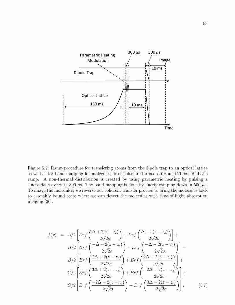
93

Time

Dipole Trap

Optical Lattice

150 ms

Image

10 ms

10 ms

500 s300 sParametric Heating

Modulation

Figure 5.2: Ramp procedure for transfering atoms from the dipole trap to an optical latticeas well as for band mapping for molecules. Molecules are formed after an 150 ms adiabaticramp. A non-thermal distribution is created by using parametric heating by pulsing asinosoidal wave with 300 µs. The band mapping is done by linerly ramping down in 500 µs.To image the molecules, we reverse our coherent transfer process to bring the molecules backto a weakly bound state where we can detect the molecules with time-of-flight absorptionimaging [26].

f(x) = A/2

[Erf

(∆ + 2(z − zc)

2√

2σ

)+ Erf

(∆− 2(z − zc)

2√

2σ

)]+

B/2

[Erf

(−∆ + 2(z − zc)

2√

2σ

)+ Erf

(−∆− 2(z − zc)

2√

2σ

)]+

B/2

[Erf

(2∆ + 2(z − zc)

2√

2σ

)+ Erf

(2∆− 2(z − zc)

2√

2σ

)]+

C/2

[Erf

(3∆ + 2(z − zc)

2√

2σ

)+ Erf

(−2∆− 2(z − zc)

2√

2σ

)]+

C/2

[Erf

(−2∆ + 2(z − zc)

2√

2σ

)+ Erf

(3∆− 2(z − zc)

2√

2σ

)], (5.7)

94

where A, B, and C, are the amplitudes of the 1st, 2nd, and 3rd Brillouin zones, d is the center

of the distribution, σ is the image resolution, and x is the variable of the function. ∆ is the

size of the distribution in the Brillouin zone, ±~k. ∆ = 2~km

Ttof

5.44µm/pix, where Ttof is the time

of flight, m is the mass of 40K87Rb, and 5.44 µm is the corresponding value in micrometers

per pixel at the image. A, B, and C, are given in units of OD (optical density). Since the

image coordinates are given in pixels, the fit gives, zc, z, ∆, and σ are all given in pixel units.

Then, the axial coordinate is converted to quasimomentum units ~k. The free parameters

of the fitting function are A, B, C, zc, and σ.

The relative population in each vibrational level of the optical lattice is given by the

area of the distribution in a momentum zone divided by the total area of the distribution.

Since these zones have the same width along the quasimomentum axis, we can use only

the amplitudes to calculate the relative population on each band. The relative molecules

population in the optical lattice are given by:

n0

ntot

=A

A + B + C, (5.8)

n1

ntot

=B

A + B + C, (5.9)

n2

ntot

=C

A + B + C, (5.10)

where, n0, n1, and n2 are the initial populations in the three first bands, and ntot is the total

initial population.

The traces in fig. 5.3 were obtained by averaging the images in the transverse direction

within one rms width of the Gaussian distribution. We fit the traces with eq. 5.7. The

uncertainty in the relative population is 3%, and is dominated by systematic errors arising

from the variation of the imaging resolution within the range of 1 to 2 pixels.

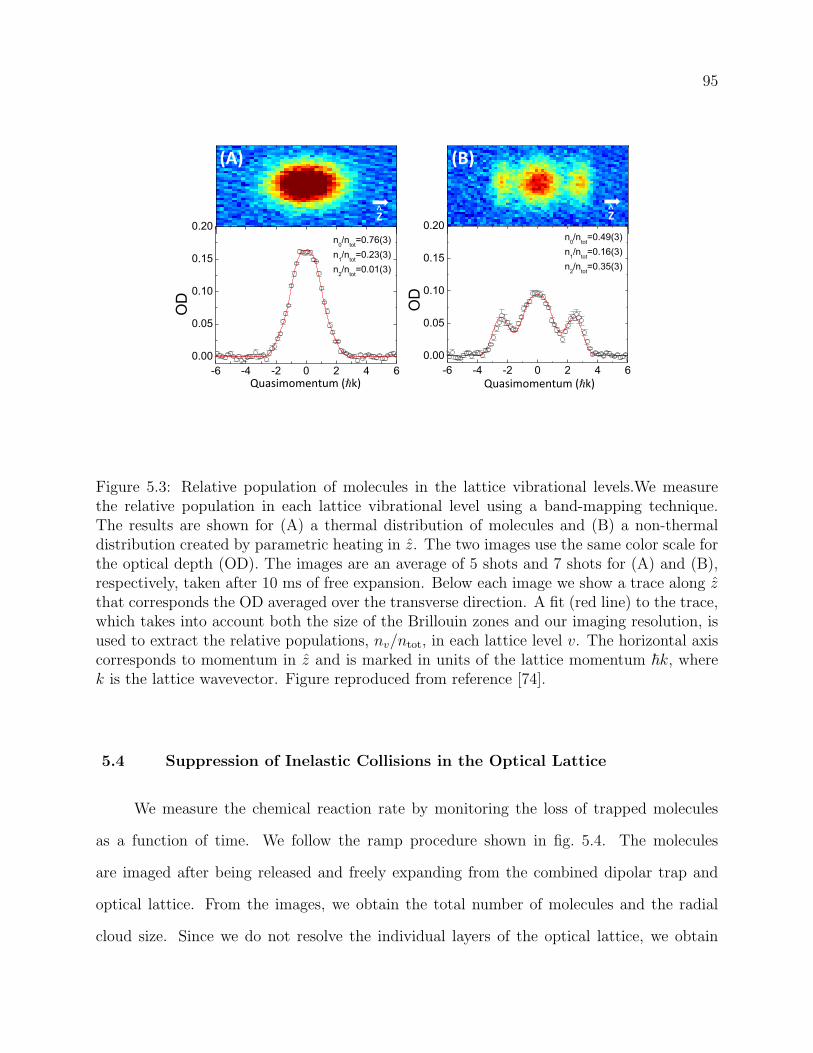
95

(A) (B)

Quasimomentum ( k) Quasimomentum ( k)

-6 -4 -2 0 2 4 6

0.00

0.05

0.10

0.15

0.20

OD

n0/n

tot=0.76(3)

n1/n

tot=0.23(3)

n2/n

tot=0.01(3)

-6 -4 -2 0 2 4 6

0.00

0.05

0.10

0.15

0.20n

0/n

tot=0.49(3)

n1/n

tot=0.16(3)

n2/n

tot=0.35(3)

OD

^Z

^Z

Figure 5.3: Relative population of molecules in the lattice vibrational levels.We measurethe relative population in each lattice vibrational level using a band-mapping technique.The results are shown for (A) a thermal distribution of molecules and (B) a non-thermaldistribution created by parametric heating in z. The two images use the same color scale forthe optical depth (OD). The images are an average of 5 shots and 7 shots for (A) and (B),respectively, taken after 10 ms of free expansion. Below each image we show a trace along zthat corresponds the OD averaged over the transverse direction. A fit (red line) to the trace,which takes into account both the size of the Brillouin zones and our imaging resolution, isused to extract the relative populations, nv/ntot, in each lattice level v. The horizontal axiscorresponds to momentum in z and is marked in units of the lattice momentum ~k, wherek is the lattice wavevector. Figure reproduced from reference [74].

5.4 Suppression of Inelastic Collisions in the Optical Lattice

We measure the chemical reaction rate by monitoring the loss of trapped molecules

as a function of time. We follow the ramp procedure shown in fig. 5.4. The molecules

are imaged after being released and freely expanding from the combined dipolar trap and

optical lattice. From the images, we obtain the total number of molecules and the radial

cloud size. Since we do not resolve the individual layers of the optical lattice, we obtain

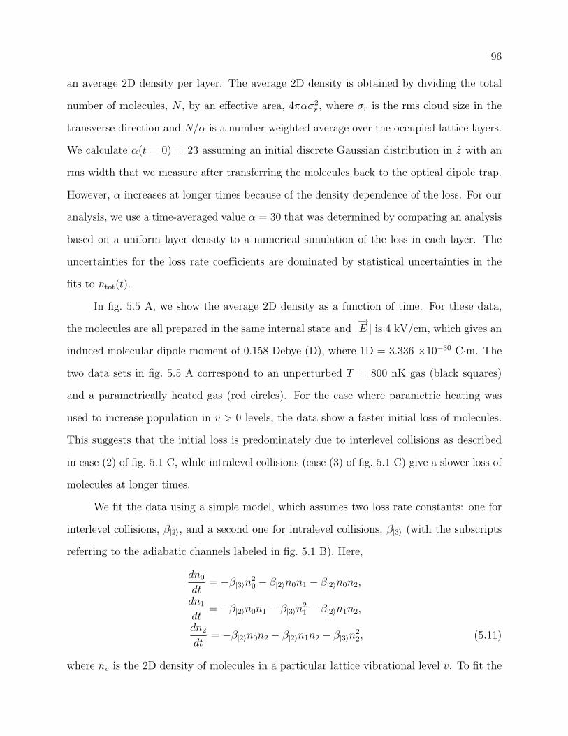
96

an average 2D density per layer. The average 2D density is obtained by dividing the total

number of molecules, N , by an effective area, 4πασ2r , where σr is the rms cloud size in the

transverse direction and N/α is a number-weighted average over the occupied lattice layers.

We calculate α(t = 0) = 23 assuming an initial discrete Gaussian distribution in z with an

rms width that we measure after transferring the molecules back to the optical dipole trap.

However, α increases at longer times because of the density dependence of the loss. For our

analysis, we use a time-averaged value α = 30 that was determined by comparing an analysis

based on a uniform layer density to a numerical simulation of the loss in each layer. The

uncertainties for the loss rate coefficients are dominated by statistical uncertainties in the

fits to ntot(t).

In fig. 5.5 A, we show the average 2D density as a function of time. For these data,

the molecules are all prepared in the same internal state and |−→E | is 4 kV/cm, which gives an

induced molecular dipole moment of 0.158 Debye (D), where 1D = 3.336 ×10−30 C·m. The

two data sets in fig. 5.5 A correspond to an unperturbed T = 800 nK gas (black squares)

and a parametrically heated gas (red circles). For the case where parametric heating was

used to increase population in v > 0 levels, the data show a faster initial loss of molecules.

This suggests that the initial loss is predominately due to interlevel collisions as described

in case (2) of fig. 5.1 C, while intralevel collisions (case (3) of fig. 5.1 C) give a slower loss of

molecules at longer times.

We fit the data using a simple model, which assumes two loss rate constants: one for

interlevel collisions, β|2〉, and a second one for intralevel collisions, β|3〉 (with the subscripts

referring to the adiabatic channels labeled in fig. 5.1 B). Here,

dn0

dt= −β|3〉n

20 − β|2〉n0n1 − β|2〉n0n2,

dn1

dt= −β|2〉n0n1 − β|3〉n

21 − β|2〉n1n2,

dn2

dt= −β|2〉n0n2 − β|2〉n1n2 − β|3〉n

22, (5.11)

where nv is the 2D density of molecules in a particular lattice vibrational level v. To fit the

97

measured time dependence of the total 2D density, ntot(t), we use ntot(t) = n0(t) + n1(t) +

n2(t). We input the measured initial populations nv/ntot (see fig. 5.3) at t = 0, and we fit

the data to the numerical solution of eq. 5.11. We obtain β|3〉 and β|2〉 from a simultaneous

fit to the two measured ntot(t) curves shown in fig. 5.5 A.

Time

Dipole Trap

Optical Lattice

150 ms

Image

10 ms

Variable

hold time

300 sParametric Heating

Modulation

5 ms

E-field on

Figure 5.4: Ramp procedure for measurement of chemical reaction rates. The40K87Rb molecules are produced when the optical lattice is fully formed at ≈ 100 Erec,after 150 ms ramp time. The molecules can be excited to higher vibrational levels of theoptical lattice via parametric heating. The parametric heating is done via a sinosoidal mod-ulation of the lattice intensity for 300 µs. The electric field is turned on together with theparametric heating and it is turned off 5 ms before we switch off the dipolar trap and theoptical lattice. The molecules are held in the combined dipolar trap and the optical latticefor a variable time. After the molecules are released from the trap, the image is taken after10 ms time of flight.

By repeating this procedure for different values of |−→E |, we measure the chemical reac-

98

tion rate constants, β|3〉 and β|2〉, as a function of the induced dipole moment. In fig. 5.5 B,

we show the intralevel (black squares) and interlevel (red circles) chemical rate constants as

a function of the dipole moment. Also shown as green triangles in fig. 5.5 B are the results

of two measurements for a 50/50 mixture of molecules in two different rotational states (case

(1) of fig. 5.1 C) |0, 0,−4, 1/2〉 and |1, 1,−4, 1/2〉. The 50/50 mixture is created by using a

π/2 microwave pulse when the molecules are in the ground state. The notation used here is∣∣N, mN ,mK

I ,mRbI

⟩, where N is the rotational quantum number, mN is the projection of the

rotational quantum number on the applied electric field direction, and mRb/KI is the nuclear

spin quantum number as in reference [65]. Here, we fit the loss of molecules in the ground

rotational state to the solution of dntot

dt= −β|1〉n2

tot to extract a single loss rate constant.

For comparison with these measurements, Goulven Qumner and John Bohn perform

quantum scattering calculations using a time-independent quantum formalism based on

spherical coordinates with cylindrical asymptotic matching to describe the molecular colli-

sions in quasi-2D [93]. We use an absorbing potential at short distance to represent chemical

reactions [42, 67]. This technique showed excellent agreement with previous experimental

data for 40K87Rb bimolecular reactions in 3D [39, 40]. We computed the loss rate coeffi-

cients βv1,v2 for molecules in different initial lattice vibrational states v1, v2, at a collision

energy of 800 nK. When the induced dipole moment is still small (0 - 0.2 D), the measured

temperature is a good approximation for the mean collision energy. The loss rates of the dif-

ferent processes can be separated into fast loss rates (β0,1, β0,2, β1,2)≈ β|2〉 and slow loss rates

(β0,0, β1,1, β2,2)≈ β|3〉. The black theoretical curve in fig. 5.5 B corresponds to an average of

the slow rates weighted by the initial populations n0, n1, n2:

βblack = β0,0 − (β0,0 − β1,1)ζ21 , (5.12)

where ζ1 = n1/ntot is the percentage of the initial relative population in the lattice vibrational

state v = 1. The red curve corresponds to the same average but for the fast rates. The green

99

curve corresponds to the loss rate of molecules in different internal states.

βred =β0,1ζ0ζ1 + β0,2ζ0ζ2 + β1,2ζ1ζ2

η0ζ1 + ζ0ζ2 + ζ1ζ2

. (5.13)

The three measured reaction rate constants shown in fig. 5.5 B are consistent with

the quantum scattering calculations for the collision channels shown in matching colors in

fig. 5.1 B and fig. 5.1 C. Molecules in different rotational states (green triangles in fig. 5.5 B)

have the highest rate for chemical reactions, consistent with the fact that they can collide

in channel |1〉, which corresponds to spatially isotropic collisions with no centrifugal barrier.

On the other hand, molecules prepared in the same internal molecular state (red circles and

black squares in fig. 5.5 B) have suppressed reaction rates because the lowest energy collision

channel (|1〉) is no longer allowed. Instead, identical molecules in different lattice levels (red

circles in fig. 5.5 B) react predominantly through collisions in channel |2〉, or “head-to-tail”,

while identical molecules in the same lattice level (black squares in fig. 5.5 B) react through

collisions in channel |3〉, or “side-by-side”. The importance of stereodynamics on the reaction

rate for polar molecules is manifest in the very different dipole-moment dependence of the

reactions rates in these two collision channels. In particular, for the case where the molecules

are prepared both in the same internal quantum state and in the same v level, the reaction

rate is suppressed even as the dipole moment is increased.

Fig. 5.6 shows how the initial loss rate in a gas of identical molecules depends on the

fractional occupation of the lowest lattice level, n0/ntot. As n0/ntot increases, the calculated

initial loss rate constant for a molecular gas in thermal equilibrium (solid black line) changes

from close to β|2〉 (the red line indicating the measured value at 0.174 D from fig. 5.5 B) to

β|3〉 (open point at n0/ntot = 1). In thermal equilibrium, the fractional occupation of the

lowest vibrational level is given by the Boltzmann distribution. For the solid black line in

fig. 5.6, the fractional molecular population f(v, T ) in a vibrational level v at temperature

T is obtained from a Boltzmann distribution, and the effective βinitial is then calculated as

βinitial = β|3〉∑

v

f(v, T )2 + β|2〉∑

v1 6=v2

f(v1, T )f(v2, T ). (5.14)

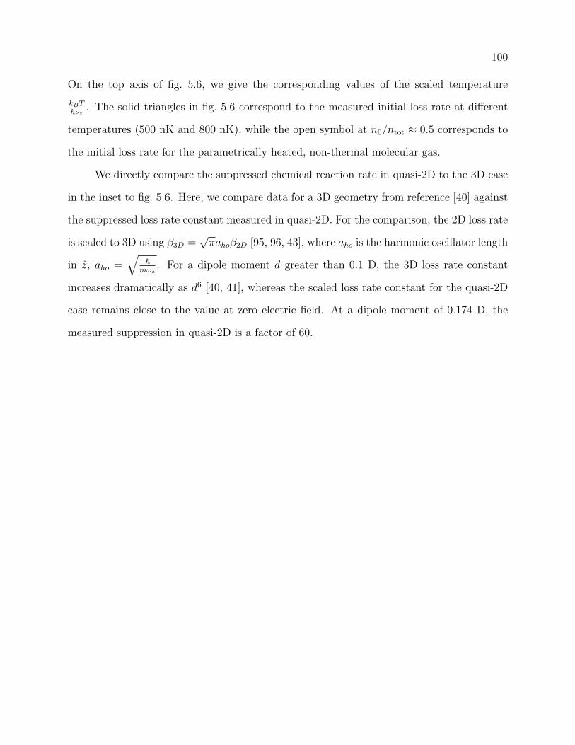
100

On the top axis of fig. 5.6, we give the corresponding values of the scaled temperature

kBThνz

. The solid triangles in fig. 5.6 correspond to the measured initial loss rate at different

temperatures (500 nK and 800 nK), while the open symbol at n0/ntot ≈ 0.5 corresponds to

the initial loss rate for the parametrically heated, non-thermal molecular gas.

We directly compare the suppressed chemical reaction rate in quasi-2D to the 3D case

in the inset to fig. 5.6. Here, we compare data for a 3D geometry from reference [40] against

the suppressed loss rate constant measured in quasi-2D. For the comparison, the 2D loss rate

is scaled to 3D using β3D =√

πahoβ2D [95, 96, 43], where aho is the harmonic oscillator length

in z, aho =√

~mωz

. For a dipole moment d greater than 0.1 D, the 3D loss rate constant

increases dramatically as d6 [40, 41], whereas the scaled loss rate constant for the quasi-2D

case remains close to the value at zero electric field. At a dipole moment of 0.174 D, the

measured suppression in quasi-2D is a factor of 60.

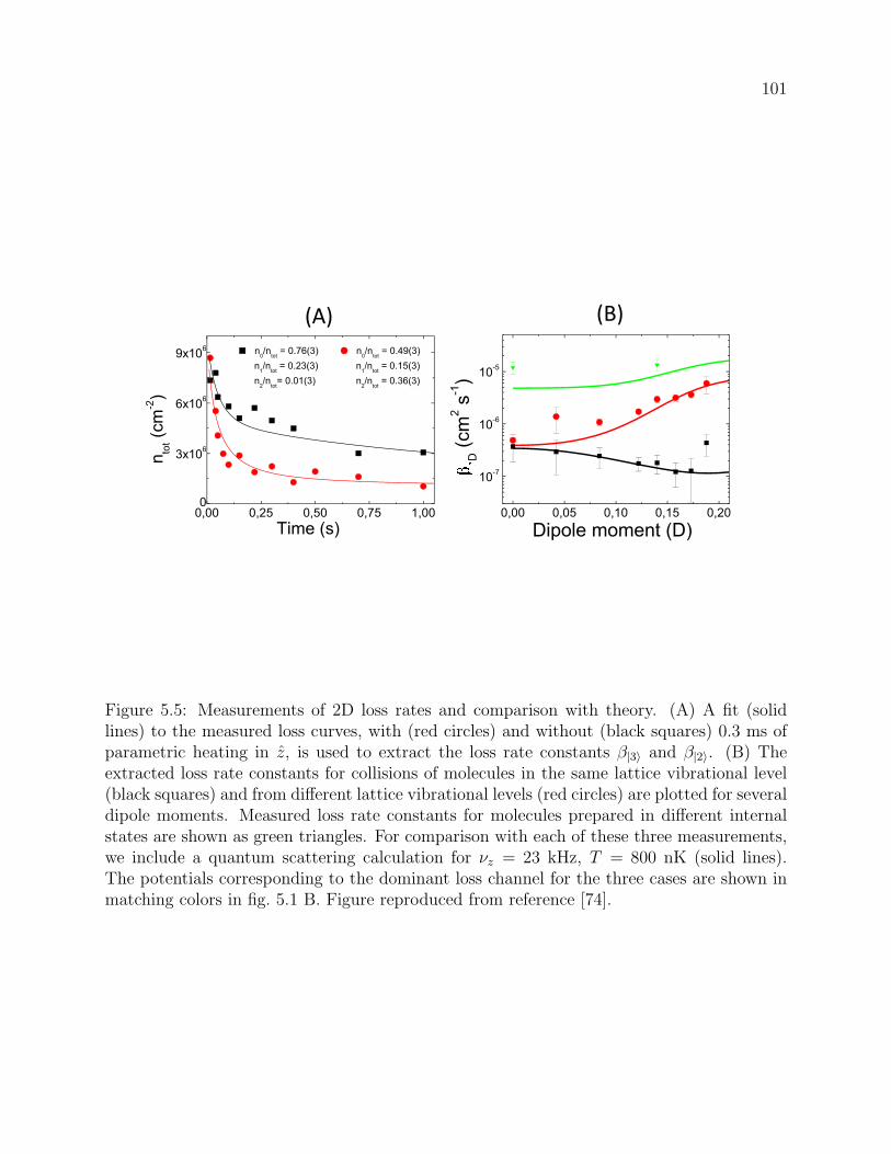
101

0,00 0,25 0,50 0,75 1,000

3x106

6x106

9x106

0,00 0,05 0,10 0,15 0,20

10-7

10-6

10-5

n0/n

tot = 0.76(3) n

0/n

tot = 0.49(3)

n1/n

tot = 0.23(3) n

1/n

tot = 0.15(3)

n2/n

tot= 0.01(3) n

2/n

tot = 0.36(3)

nto

t (cm

-2)

Time (s) Dipole moment (D)

D (

cm

2 s

-1)

(B)(A)

Figure 5.5: Measurements of 2D loss rates and comparison with theory. (A) A fit (solidlines) to the measured loss curves, with (red circles) and without (black squares) 0.3 ms ofparametric heating in z, is used to extract the loss rate constants β|3〉 and β|2〉. (B) Theextracted loss rate constants for collisions of molecules in the same lattice vibrational level(black squares) and from different lattice vibrational levels (red circles) are plotted for severaldipole moments. Measured loss rate constants for molecules prepared in different internalstates are shown as green triangles. For comparison with each of these three measurements,we include a quantum scattering calculation for νz = 23 kHz, T = 800 nK (solid lines).The potentials corresponding to the dominant loss channel for the three cases are shown inmatching colors in fig. 5.1 B. Figure reproduced from reference [74].

102

0.5 0.6 0.7 0.8 0.9 1.0

10-7

10-6

10-5

0.00 0.05 0.10 0.15 0.2010

-13

10-12

10-11

10-10

10-9

D

(cm

3s

-1)

Dipole moment (D)

11.5 0in

itia

l(cm

2 s

-1)

n0/n

tot

kBT/ h

z 0.5

Figure 5.6: Loss rates from 3D to 2D. The effective initial loss rate, βinitial, for polar moleculesconfined in a 2D geometry depends on the fractional population (n0/ntot) in the lowestharmonic oscillator level in z, which for a gas in thermal equilibrium depends on the ratiokBThνz

. The measured initial loss rates for a dipole moment of 0.174 D are displayed for twodifferent thermal distributions (solid triangles), a non-thermal sample created by parametricheating (the top open triangle), and an extracted pure β|3〉 when the entire population isresiding in the lattice ground vibrational level (the bottom open triangle). The experimentalresults agree well with a simple model (black curve) described in this section. The top lineindicates the value of β|2〉 as measured in fig. 5.5 B. (Inset) The intralevel loss rate foridentical fermionic 40K87Rb molecules in 2D (black circles) is compared with the loss rate in3D (blue triangles). The 3D data for T = 300 nK are borrowed from reference [40]. The 2Ddata were taken at T = 800 nK and are converted to 3D rates by multiplication with

√πaho,

where aho is the harmonic oscillator length in z. Figure reproduced from reference [74].

Chapter 6

Conclusion and Future Work

6.1 Conclusion

In this thesis I have presented experimental advances of a dense, ultracold, and near

quantum degenerate polar gas of 40K87Rb. For dipolar molecules in a 3D geometry, the

chemical reaction loss was seen scale with the dipole moment to the power of six [40], due

to attractive dipole-dipole interactions via “head-to-tail” collisions. The main result demon-

strated in this thesis is that the inelastic collisions can be suppressed when the molecules

are confined in a quasi-2D geometry in a one-dimensional optical lattice. Compared to

dipole-dipole collisions in 3D geometry, collisions in quasi-2D geometry under appropriate

state preparations can suppress the inelastic loss by about two orders of magnitude [74]. We

control the population in the optical lattice of the motional states, which makes it possible

to observe collisions with single components of the p-partial wave.

6.2 Future work

For future work with these 40K87Rb molecules there are many possibilities for new

exciting experiments:

• Anisotropic rethermalization: observe rethermalization of the molecular cloud be-

tween the two transverse directions (x and y) in this 2D geometry.

• Measurement of the elastic cross section of molecules: when the molecular cloud

104

rethermalizes. We can directly measure the rate of rethermalization as a function of

the dipole moment. This will let us determine the elastic cross section for dipolar

collisions as proposed by Bohn et al. [72].

• Realization of quantum degenerate polar gas of 40K87Rb: With the first two steps

accomplished, it is possible to reach quantum degenerate regime for a gas of polar

molecules via evaporative cooling.

• Detection of chemical reaction products: so far, we only detect molecular loss. How-

ever, the vacuum chamber could be designed with an ion detector to enable detection

of ultracold chemical reactions products.

• Detecting novel quantum phases in the geometry of stacked 2D traps [33, 34, 35, 97,

88, 98].

Bibliography

[1] K.-K. Ni, S. Ospelkaus, D. Wang, G. Quemener, B. Neyenhuis, M. H. G. de Miranda,J. L. Bohn, J. Ye, and D. S. Jin, Dipolar collisions of polar molecules in the quantumregime, Nature 464, 1324 (2010).

[2] K.-K. Ni, S. Ospelkaus, M. H. G. de Miranda, A. Pe’er, B. Neyenhuis, J. J. Zirbel, S.Kotochigova, P. S. Julienne, D. S. Jin, and J. Ye, A High Phase-Space-Density Gas ofPolar Molecules, Science 322, 231 (2008).

[3] K. W. Holman, Distribution of an Ultrastable Frequency Reference Using Optical Fre-quency Combs, Ph.D. thesis, University of Colorado at Boulder, 2005.

[4] S. Ospelkaus, K.-K. Ni, M. H. G. de Miranda, B. Neyenhuis, D. Wang, S. Kotochigova,P. S. Julienne, D. S. Jin, and J. Ye, Ultracold polar molecules near quantum degeneracy,Faraday Discussions 142, 351 (2008).

[5] S. Ospelkaus, K.-K. Ni, D. Wang, M. H. G. de Miranda, B. Neyenhuis, G. Quemener,P. S. Julienne, J. L. Bohn, D. S. Jin, and J. Ye, Quantum-State Controlled UltracoldChemistry, Science 327, 853 (2010).

[6] M. H. G. de Miranda, A. Chotia, B. Neyenhuis, D. Wang, G. Quemener, S. Ospelkaus,J. L. Bohn, J. Ye, and D. S. Jin, Controlling the quantum stereodynamics of ultracoldbimolecular reactions, (submitted. (2010)).

[7] C. N. Cohen-Tannoudji, Nobel Lecture: Manipulating atoms with photons, Rev. Mod.Phys. 70, 707 (1998).

[8] S. Chu, Nobel Lecture: The manipulation of neutral particles, Rev. Mod. Phys. 70, 685(1998).

[9] W. D. Phillips, Nobel Lecture: Laser cooling and trapping of neutral atoms, Rev. Mod.Phys. 70, 721 (1998).

[10] M. H. Anderson, J. R. Ensher, M. R. Matthews, C. E. Wieman, and E. A. Cornell,Observation of Bose-Einstein Condensation in a Dilute Atomic Vapor, Science 269, 198(1995).

106

[11] W. Ketterle, Nobel lecture: When atoms behave as waves: Bose-Einstein condensationand the atom laser, Rev. Mod. Phys. 74, 1131 (2002).

[12] E. A. Cornell and C. E. Wieman, Nobel Lecture: Bose-Einstein condensation in a dilutegas, the first 70 years and some recent experiments, Rev. Mod. Phys. 74, 875 (2002).

[13] K. B. Davis, M. O. Mewes, M. R. Andrews, N. J. van Druten, D. S. Durfee, D. M.Kurn, and W. Ketterle, Bose-Einstein Condensation in a Gas of Sodium Atoms, Phys.Rev. Lett. 75, 3969 (1995).

[14] B. DeMarco and D. S. Jin, Onset of Fermi Degeneracy in a Trapped Atomic Gas, Science285, 1703 (1999).

[15] S. Inouye, M. R. Andrews, J. Stenger, H.-J. Miesner, D. M. Stamper-Kurn, and W.Ketterle, Observation of Feshbach resonances in a Bose-Einstein condensate, Nature392, 151 (1998).

[16] C. A. Regal, M. Greiner, and D. S. Jin, Observation of Resonance Condensation ofFermionic Atom Pairs, Phys. Rev. Lett. 92, 040403 (2004).

[17] M. W. Zwierlein, C. A. Stan, C. H. Schunck, S. M. F. Raupach, A. J. Kerman, and W.Ketterle, Condensation of Pairs of Fermionic Atoms near a Feshbach Resonance, Phys.Rev. Lett. 92, 120403 (2004).

[18] M. Bartenstein, A. Altmeyer, S. Riedl, S. Jochim, C. Chin, J. H. Denschlag, and R.Grimm, Collective Excitations of a Degenerate Gas at the BEC-BCS Crossover, Phys.Rev. Lett. 92, 203201 (2004).

[19] E. A. Donley, N. R. Claussen, S. T. Thompson, and C. E. Wieman, Atom-moleculecoherence in a Bose-Einstein condensate, Nature 417, 529 (2002).

[20] C. Chin, A. J. Kerman, V. Vuletic, and S. Chu, Sensitive Detection of Cold CesiumMolecules Formed on Feshbach Resonances, Phys. Rev. Lett. 90, 033201 (2003).

[21] S. Y. T. van de Meerakker, P. H. M. Smeets, N. Vanhaecke, R. T. Jongma, and G.Meijer, Deceleration and Electrostatic Trapping of OH Radicals, Phys. Rev. Lett. 94,023004 (2005).

[22] M. T. Hummon, W. C. Campbell, H.-I. Lu, E. Tsikata, Y. Wang, and J. M. Doyle,Magnetic trapping of atomic nitrogen (N14) and cotrapping of NH (XΣ − 3), Phys.Rev. A 78, 050702 (2008).

[23] B. C. Sawyer, B. K. Stuhl, D. Wang, M. Yeo, and J. Ye, Molecular Beam Collisionswith a Magnetically Trapped Target, Phys. Rev. Lett. 101, 203203 (2008).

[24] J. M. Sage, S. Sainis, T. Bergeman, and D. DeMille, Optical Production of UltracoldPolar Molecules, Phys. Rev. Lett. 94, 203001 (2005).

107

[25] K. Bergmann, H. Theuer, and B. W. Shore, Coherent population transfer among quan-tum states of atoms and molecules, Rev. Mod. Phys. 70, 1003 (1998).

[26] A. Pe’er, E. A. Shapiro, M. C. Stowe, M. Shapiro, and J. Ye, Precise Control of MolecularDynamics with a Femtosecond Frequency Comb, Phys. Rev. Lett. 98, 113004 (2007).

[27] K.-K. Ni, A Quantum Gas of Polar Molecules, Ph.D. thesis, University of Colorado atBoulder, 2009.

[28] T. Kohler, K. Goral, and P. S. Julienne, Production of cold molecules via magneticallytunable Feshbach resonances, Rev. Mod. Phys. 78, 1311 (2006).

[29] S. Ospelkaus, A. Peer, K.-K. Ni, J. J. Zirbel, B. Neyenhuis, S. Kotochigova, P. S.Julienne, J. Ye, and D. S. Jin, Efficient state transfer in an ultracold dense gas ofheteronuclear molecules, Nat Phys 4, 622 (2008).

[30] J. G. Danzl, E. Haller, M. Gustavsson, M. J. Mark, R. Hart, N. Bouloufa, O. Dulieu,H. Ritsch, and H.-C. Nagerl, Quantum Gas of Deeply Bound Ground State Molecules,Science 321, 1062 (2008).

[31] F. Lang, K. Winkler, C. Strauss, R. Grimm, and J. H. Denschlag, Ultracold TripletMolecules in the Rovibrational Ground State, Phys. Rev. Lett. 101, 133005 (2008).

[32] T. Udem, J. Reichert, R. Holzwarth, and T. W. Hansch, Absolute Optical FrequencyMeasurement of the Cesium D1 Line with a Mode-Locked Laser, Phys. Rev. Lett. 82,3568 (1999).

[33] D. J. Jones, S. A. Diddams, J. K. Ranka, A. Stentz, R. S. Windeler, J. L. Hall, andS. T. Cundiff, Carrier-Envelope Phase Control of Femtosecond Mode-Locked Lasers andDirect Optical Frequency Synthesis, Science 288, 635 (2000).

[34] S. T. Cundiff and J. Ye, Colloquium: Femtosecond optical frequency combs, Rev. Mod.Phys. 75, 325 (2003).

[35] F. Dalfovo, S. Giorgini, L. P. Pitaevskii, and S. Stringari, Theory of Bose-Einsteincondensation in trapped gases, Rev. Mod. Phys. 71, 463 (1999).

[36] J. Stuhler, A. Griesmaier, T. Koch, M. Fattori, T. Pfau, S. Giovanazzi, P. Pedri, and L.Santos, Observation of Dipole-Dipole Interaction in a Degenerate Quantum Gas, Phys.Rev. Lett. 95, 150406 (2005).

[37] T. Lahaye, T. Koch, B. Frohlich, M. Fattori, J. Metz, A. Griesmaier, S. Giovanazzi, andT. Pfau, Strong dipolar effects in a quantum ferrofluid, Nature 448, 672 (2007).

[38] H. P. Buchler, E. Demler, M. Lukin, A. Micheli, N. Prokof’ev, G. Pupillo, and P. Zoller,Strongly Correlated 2D Quantum Phases with Cold Polar Molecules: Controlling theShape of the Interaction Potential, Phys. Rev. Lett. 98, 060404 (2007).

108

[39] L. Santos, G. V. Shlyapnikov, P. Zoller, and M. Lewenstein, Bose-Einstein Condensationin Trapped Dipolar Gases, Phys. Rev. Lett. 85, 1791 (2000).

[40] G. Pupillo, A. Micheli, H. P. Buchler, and P. Zoller, Cold Molecules: Theory, Experi-ment, Applications (Taylor & Francis, Boca Raton, 2009).

[41] D. DeMille, Quantum Computation with Trapped Polar Molecules, Phys. Rev. Lett. 88,067901 (2002).

[42] S. F. Yelin, K. Kirby, and R. Cote, Schemes for robust quantum computation with polarmolecules, Phys. Rev. A 74, 050301 (2006).

[43] A. Andre, D. DeMille, J. M. Doyle, M. D. Lukin, S. E. Maxwell, P. Rabl, R. J.Schoelkopf, and P. Zoller, A coherent all-electrical interface between polar moleculesand mesoscopic superconducting resonators, Nat Phys 2, 636 (2006).

[44] G. Quemener and J. L. Bohn, Strong dependence of ultracold chemical rates on electricdipole moments, Phys. Rev. A 81, 022702 (2010).

[45] G. Quemener and J. L. Bohn, Electric field suppression of ultracold confined chemicalreactions, Phys. Rev. A 81, 060701 (2010).

[46] A. Micheli, Z. Idziaszek, G. Pupillo, M. A. Baranov, P. Zoller, and P. S. Julienne,Universal Rates for Reactive Ultracold Polar Molecules in Reduced Dimensions, Phys.Rev. Lett. 105, 073202 (2010).

[47] J. J. Zirbel, K.-K. Ni, S. Ospelkaus, T. L. Nicholson, M. L. Olsen, P. S. Julienne, C. E.Wieman, J. Ye, and D. S. Jin, Heteronuclear molecules in an optical dipole trap, Phys.Rev. A 78, 013416 (2008).

[48] J. Zirbel, Ultracold Fermionic Feshbach Molecules, Ph.D. thesis, University of Coloradoat Boulder, 2008.

[49] S. Ospelkaus, C. Ospelkaus, L. Humbert, K. Sengstock, and K. Bongs, Tuning of Het-eronuclear Interactions in a Degenerate Fermi-Bose Mixture, Phys. Rev. Lett. 97, 120403(2006).

[50] J. J. Zirbel, K.-K. Ni, S. Ospelkaus, J. P. D’Incao, C. E. Wieman, J. Ye, and D. S. Jin,Collisional Stability of Fermionic Feshbach Molecules, Phys. Rev. Lett. 100, 143201(2008).

[51] A. Marian, M. C. Stowe, J. R. Lawall, D. Felinto, and J. Ye, United Time-FrequencySpectroscopy for Dynamics and Global Structure, Science 306, 2063 (2004).

[52] M. J. Thorpe, K. D. Moll, R. J. Jones, B. Safdi, and J. Ye, Broadband Cavity RingdownSpectroscopy for Sensitive and Rapid Molecular Detection, Science 311, 1595 (2006).

[53] A. D. Ludlow et al., Sr Lattice Clock at 1 x 10-16 Fractional Uncertainty by RemoteOptical Evaluation with a Ca Clock, Science 319, 1805 (2008).

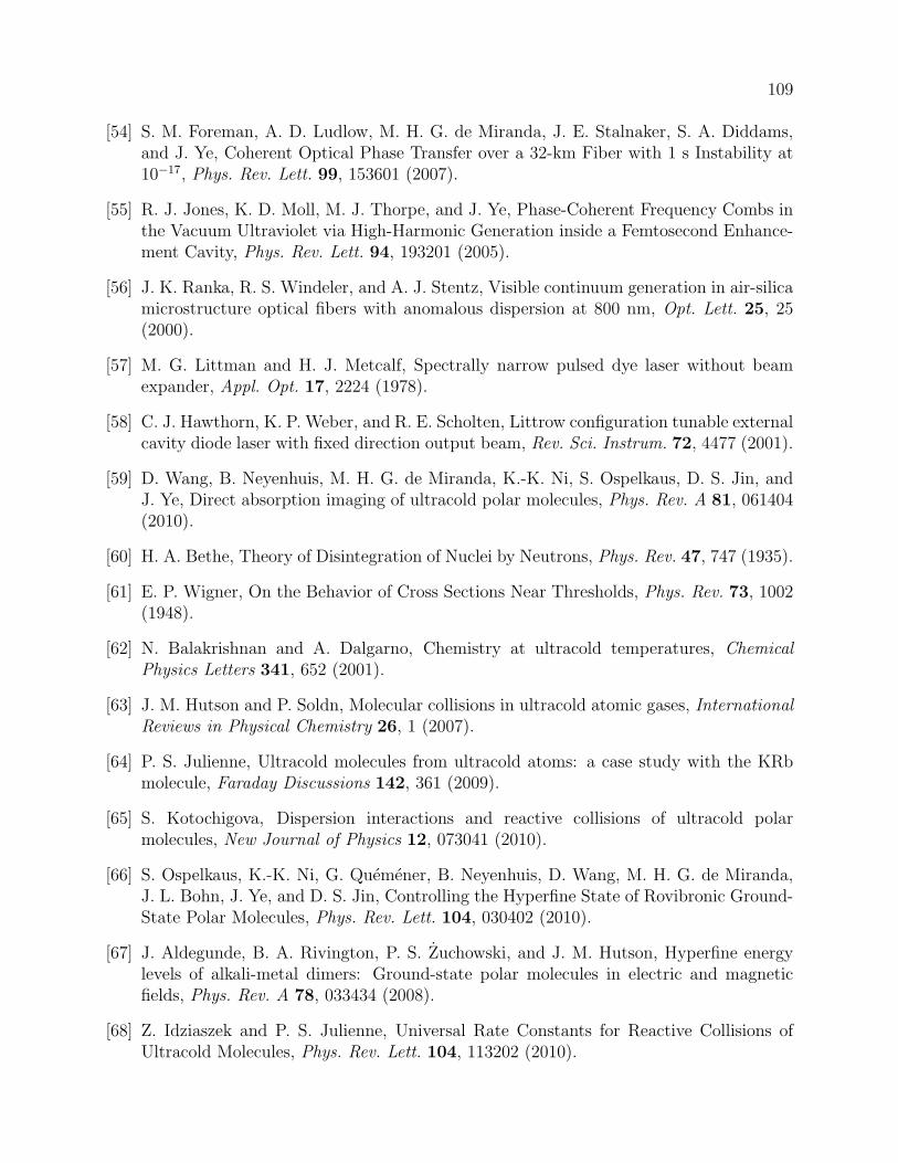
109

[54] S. M. Foreman, A. D. Ludlow, M. H. G. de Miranda, J. E. Stalnaker, S. A. Diddams,and J. Ye, Coherent Optical Phase Transfer over a 32-km Fiber with 1 s Instability at10−17, Phys. Rev. Lett. 99, 153601 (2007).

[55] R. J. Jones, K. D. Moll, M. J. Thorpe, and J. Ye, Phase-Coherent Frequency Combs inthe Vacuum Ultraviolet via High-Harmonic Generation inside a Femtosecond Enhance-ment Cavity, Phys. Rev. Lett. 94, 193201 (2005).

[56] J. K. Ranka, R. S. Windeler, and A. J. Stentz, Visible continuum generation in air-silicamicrostructure optical fibers with anomalous dispersion at 800 nm, Opt. Lett. 25, 25(2000).

[57] M. G. Littman and H. J. Metcalf, Spectrally narrow pulsed dye laser without beamexpander, Appl. Opt. 17, 2224 (1978).

[58] C. J. Hawthorn, K. P. Weber, and R. E. Scholten, Littrow configuration tunable externalcavity diode laser with fixed direction output beam, Rev. Sci. Instrum. 72, 4477 (2001).

[59] D. Wang, B. Neyenhuis, M. H. G. de Miranda, K.-K. Ni, S. Ospelkaus, D. S. Jin, andJ. Ye, Direct absorption imaging of ultracold polar molecules, Phys. Rev. A 81, 061404(2010).

[60] H. A. Bethe, Theory of Disintegration of Nuclei by Neutrons, Phys. Rev. 47, 747 (1935).

[61] E. P. Wigner, On the Behavior of Cross Sections Near Thresholds, Phys. Rev. 73, 1002(1948).

[62] N. Balakrishnan and A. Dalgarno, Chemistry at ultracold temperatures, ChemicalPhysics Letters 341, 652 (2001).

[63] J. M. Hutson and P. Soldn, Molecular collisions in ultracold atomic gases, InternationalReviews in Physical Chemistry 26, 1 (2007).

[64] P. S. Julienne, Ultracold molecules from ultracold atoms: a case study with the KRbmolecule, Faraday Discussions 142, 361 (2009).

[65] S. Kotochigova, Dispersion interactions and reactive collisions of ultracold polarmolecules, New Journal of Physics 12, 073041 (2010).

[66] S. Ospelkaus, K.-K. Ni, G. Quemener, B. Neyenhuis, D. Wang, M. H. G. de Miranda,J. L. Bohn, J. Ye, and D. S. Jin, Controlling the Hyperfine State of Rovibronic Ground-State Polar Molecules, Phys. Rev. Lett. 104, 030402 (2010).

[67] J. Aldegunde, B. A. Rivington, P. S. Zuchowski, and J. M. Hutson, Hyperfine energylevels of alkali-metal dimers: Ground-state polar molecules in electric and magneticfields, Phys. Rev. A 78, 033434 (2008).

[68] Z. Idziaszek and P. S. Julienne, Universal Rate Constants for Reactive Collisions ofUltracold Molecules, Phys. Rev. Lett. 104, 113202 (2010).

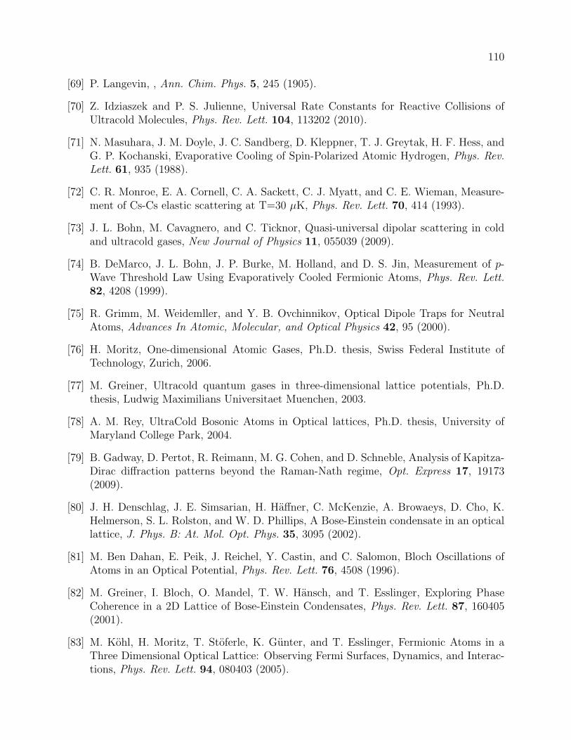
110

[69] P. Langevin, , Ann. Chim. Phys. 5, 245 (1905).

[70] Z. Idziaszek and P. S. Julienne, Universal Rate Constants for Reactive Collisions ofUltracold Molecules, Phys. Rev. Lett. 104, 113202 (2010).

[71] N. Masuhara, J. M. Doyle, J. C. Sandberg, D. Kleppner, T. J. Greytak, H. F. Hess, andG. P. Kochanski, Evaporative Cooling of Spin-Polarized Atomic Hydrogen, Phys. Rev.Lett. 61, 935 (1988).

[72] C. R. Monroe, E. A. Cornell, C. A. Sackett, C. J. Myatt, and C. E. Wieman, Measure-ment of Cs-Cs elastic scattering at T=30 µK, Phys. Rev. Lett. 70, 414 (1993).

[73] J. L. Bohn, M. Cavagnero, and C. Ticknor, Quasi-universal dipolar scattering in coldand ultracold gases, New Journal of Physics 11, 055039 (2009).

[74] B. DeMarco, J. L. Bohn, J. P. Burke, M. Holland, and D. S. Jin, Measurement of p-Wave Threshold Law Using Evaporatively Cooled Fermionic Atoms, Phys. Rev. Lett.82, 4208 (1999).

[75] R. Grimm, M. Weidemller, and Y. B. Ovchinnikov, Optical Dipole Traps for NeutralAtoms, Advances In Atomic, Molecular, and Optical Physics 42, 95 (2000).

[76] H. Moritz, One-dimensional Atomic Gases, Ph.D. thesis, Swiss Federal Institute ofTechnology, Zurich, 2006.

[77] M. Greiner, Ultracold quantum gases in three-dimensional lattice potentials, Ph.D.thesis, Ludwig Maximilians Universitaet Muenchen, 2003.

[78] A. M. Rey, UltraCold Bosonic Atoms in Optical lattices, Ph.D. thesis, University ofMaryland College Park, 2004.

[79] B. Gadway, D. Pertot, R. Reimann, M. G. Cohen, and D. Schneble, Analysis of Kapitza-Dirac diffraction patterns beyond the Raman-Nath regime, Opt. Express 17, 19173(2009).

[80] J. H. Denschlag, J. E. Simsarian, H. Haffner, C. McKenzie, A. Browaeys, D. Cho, K.Helmerson, S. L. Rolston, and W. D. Phillips, A Bose-Einstein condensate in an opticallattice, J. Phys. B: At. Mol. Opt. Phys. 35, 3095 (2002).

[81] M. Ben Dahan, E. Peik, J. Reichel, Y. Castin, and C. Salomon, Bloch Oscillations ofAtoms in an Optical Potential, Phys. Rev. Lett. 76, 4508 (1996).

[82] M. Greiner, I. Bloch, O. Mandel, T. W. Hansch, and T. Esslinger, Exploring PhaseCoherence in a 2D Lattice of Bose-Einstein Condensates, Phys. Rev. Lett. 87, 160405(2001).

[83] M. Kohl, H. Moritz, T. Stoferle, K. Gunter, and T. Esslinger, Fermionic Atoms in aThree Dimensional Optical Lattice: Observing Fermi Surfaces, Dynamics, and Interac-tions, Phys. Rev. Lett. 94, 080403 (2005).

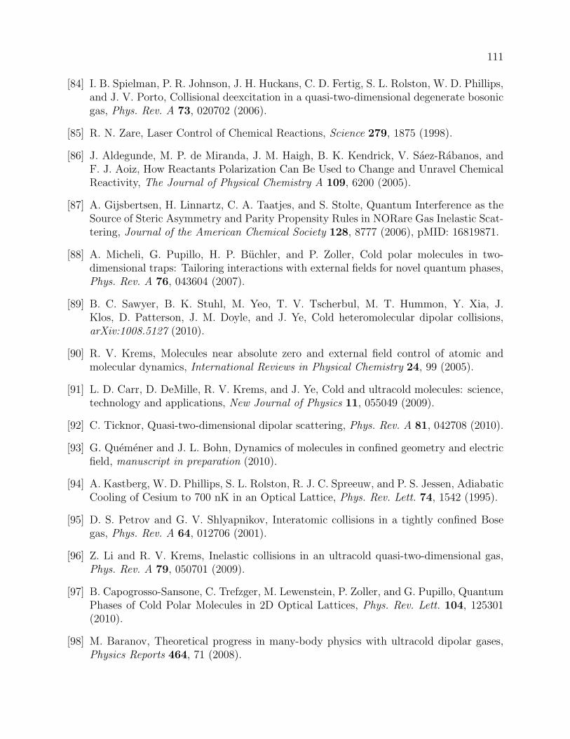
111

[84] I. B. Spielman, P. R. Johnson, J. H. Huckans, C. D. Fertig, S. L. Rolston, W. D. Phillips,and J. V. Porto, Collisional deexcitation in a quasi-two-dimensional degenerate bosonicgas, Phys. Rev. A 73, 020702 (2006).

[85] R. N. Zare, Laser Control of Chemical Reactions, Science 279, 1875 (1998).

[86] J. Aldegunde, M. P. de Miranda, J. M. Haigh, B. K. Kendrick, V. Saez-Rabanos, andF. J. Aoiz, How Reactants Polarization Can Be Used to Change and Unravel ChemicalReactivity, The Journal of Physical Chemistry A 109, 6200 (2005).

[87] A. Gijsbertsen, H. Linnartz, C. A. Taatjes, and S. Stolte, Quantum Interference as theSource of Steric Asymmetry and Parity Propensity Rules in NORare Gas Inelastic Scat-tering, Journal of the American Chemical Society 128, 8777 (2006), pMID: 16819871.

[88] A. Micheli, G. Pupillo, H. P. Buchler, and P. Zoller, Cold polar molecules in two-dimensional traps: Tailoring interactions with external fields for novel quantum phases,Phys. Rev. A 76, 043604 (2007).

[89] B. C. Sawyer, B. K. Stuhl, M. Yeo, T. V. Tscherbul, M. T. Hummon, Y. Xia, J.Klos, D. Patterson, J. M. Doyle, and J. Ye, Cold heteromolecular dipolar collisions,arXiv:1008.5127 (2010).

[90] R. V. Krems, Molecules near absolute zero and external field control of atomic andmolecular dynamics, International Reviews in Physical Chemistry 24, 99 (2005).

[91] L. D. Carr, D. DeMille, R. V. Krems, and J. Ye, Cold and ultracold molecules: science,technology and applications, New Journal of Physics 11, 055049 (2009).

[92] C. Ticknor, Quasi-two-dimensional dipolar scattering, Phys. Rev. A 81, 042708 (2010).

[93] G. Quemener and J. L. Bohn, Dynamics of molecules in confined geometry and electricfield, manuscript in preparation (2010).

[94] A. Kastberg, W. D. Phillips, S. L. Rolston, R. J. C. Spreeuw, and P. S. Jessen, AdiabaticCooling of Cesium to 700 nK in an Optical Lattice, Phys. Rev. Lett. 74, 1542 (1995).

[95] D. S. Petrov and G. V. Shlyapnikov, Interatomic collisions in a tightly confined Bosegas, Phys. Rev. A 64, 012706 (2001).

[96] Z. Li and R. V. Krems, Inelastic collisions in an ultracold quasi-two-dimensional gas,Phys. Rev. A 79, 050701 (2009).

[97] B. Capogrosso-Sansone, C. Trefzger, M. Lewenstein, P. Zoller, and G. Pupillo, QuantumPhases of Cold Polar Molecules in 2D Optical Lattices, Phys. Rev. Lett. 104, 125301(2010).

[98] M. Baranov, Theoretical progress in many-body physics with ultracold dipolar gases,Physics Reports 464, 71 (2008).