Continuous Time Markov Chain approximation of the Heston model · Time Markov Chain (CTMC) approximation to the variance process. The new formulation enables a closed-form solution

Continuous Time Markov Chain approximation of theHeston model

Alvaro Leitao, Justin L. Kirkby and Luis Ortiz-Gracia

ICCF 2019

July 12, 2019

A. Leitao & J.L. Kirkby & L. Ortiz-Gracia CTMC-Heston model July 12, 2019 1 / 30

Motivation

The Heston model is a widely utilized stochastic volatility (SV)models in the option pricing literature as well as in practice.

For a fixed time horizon, the characteristic function (ChF) is known inclosed-form.

Then, European option pricing is efficiently accomplished with anystandard Fourier method.

Enabling a fast calibration of the Heston model parameters to matchobserved volatility surfaces, as required in practice.

However, after calibration there is still great difficulty in pricing exoticcontracts under the Heston model.

To price contracts such as Asian options and variance swaps, MonteCarlo (MC) methods are the traditional surrogates in these cases.

Unfortunately, MC suffers from a number of well known deficiencies,and complicated simulation schemes are often required to overcomethe boundary effects that accompany models such as Heston.


What we propose

The practical objective of this work is to formalize a model whichreproduces vanilla market quotes, but is at the same time amenableto complex derivative pricing in a manner that is consistent with thecalibrated model.

We propose a model and framework based on the Heston model. Wecall this the CTMC-Heston model, as it uses a finite state ContinuousTime Markov Chain (CTMC) approximation to the variance process.

The new formulation enables a closed-form solution for the ChF ofthe underlying (log-)returns, which allows the use of Fourier inversiontechniques to efficiently price exotics.

We provide numerical studies which demonstrate convergence toHeston’s model as the state space is refined. A detailed theoreticalanalysis of the method will follow.


Outline

1 From Heston model to CTMC-Heston model

2 Calibration of the CTMC-Heston model

3 Application: Pricing Exotic options under CTMC-Heston model

4 Conclusions


From Heston model to CTMC-Heston model

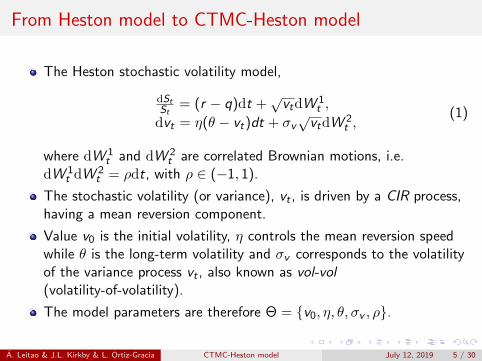
The Heston stochastic volatility model,

dStSt

= (r − q)dt +√vtdW

1t ,

dvt = η(θ − vt)dt + σv√vtdW

2t ,

(1)

where dW 1t and dW 2

t are correlated Brownian motions, i.e.dW 1

t dW2t = ρdt, with ρ ∈ (−1, 1).

The stochastic volatility (or variance), vt , is driven by a CIR process,having a mean reversion component.

Value v0 is the initial volatility, η controls the mean reversion speedwhile θ is the long-term volatility and σv corresponds to the volatilityof the variance process vt , also known as vol-vol(volatility-of-volatility).

The model parameters are therefore Θ = {v0, η, θ, σv , ρ}.


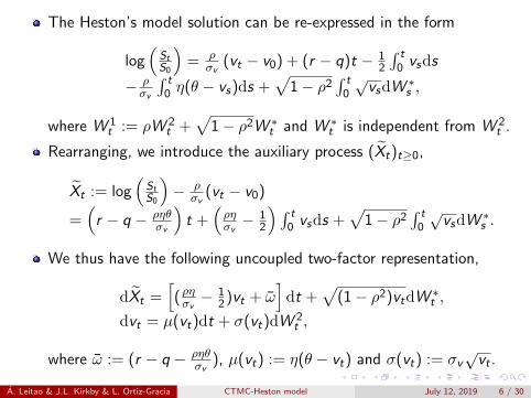
The Heston’s model solution can be re-expressed in the form

log(StS0

)= ρ

σv(vt − v0) + (r − q)t − 1

2

∫ t0 vsds

− ρσv

∫ t0 η(θ − vs)ds +

√1− ρ2

∫ t0

√vsdW

∗s ,

where W 1t := ρW 2

t +√

1− ρ2W ∗t and W ∗

t is independent from W 2t .

Rearranging, we introduce the auxiliary process (Xt)t≥0,

Xt := log(StS0

)− ρ

σv(vt − v0)

=(r − q − ρηθ

σv

)t +

(ρησv− 1

2

) ∫ t0 vsds +

√1− ρ2

∫ t0

√vsdW

∗s .

We thus have the following uncoupled two-factor representation,

dXt =[(ρησv −

12 )vt + ω

]dt +

√(1− ρ2)vtdW

∗t ,

dvt = µ(vt)dt + σ(vt)dW2t ,

where ω := (r − q − ρηθσv

), µ(vt) := η(θ − vt) and σ(vt) := σv√vt .


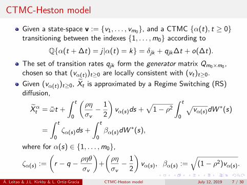
CTMC-Heston model

Given a state-space v := {v1, . . . , vm0}, and a CTMC {α(t), t ≥ 0}transitioning between the indexes {1, . . . ,m0} according to

Q{α(t + ∆t) = j |α(t) = k} = δjk + qjk∆t + o(∆t).

The set of transition rates qjk form the generator matrix Qm0×m0 ,chosen so that (vα(t))t≥0 are locally consistent with (vt)t≥0.

Given (vα(t))t≥0, Xt is approximated by a Regime Switching (RS)diffusion,

Xαt = ωt +

∫ t

0

(ρη

σv− 1

2

)vα(s)ds +

√1− ρ2

∫ t

0

√vα(s)dW

∗(s)

=

∫ t

0ζα(s)ds +

∫ t

0βα(s)dW

∗(s),

where for α(s) ∈ {1, . . . ,m0},

ζα(s) :=

(r − q − ρηθ

σv

)+

(ρη

σv− 1

2

)vα(s), βα(s) :=

√(1− ρ2)vα(s).


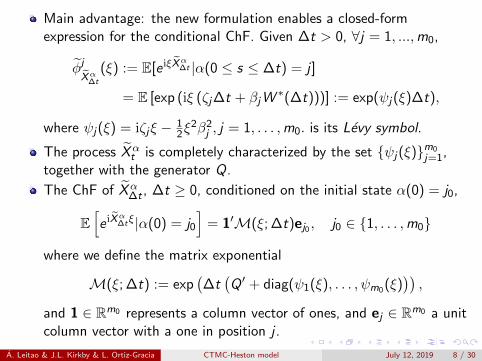
Main advantage: the new formulation enables a closed-formexpression for the conditional ChF. Given ∆t > 0, ∀j = 1, ...,m0,

φjXα

∆t

(ξ) := E[e iξXα∆t |α(0 ≤ s ≤ ∆t) = j ]

= E [exp (iξ (ζj∆t + βjW∗(∆t)))] := exp(ψj(ξ)∆t),

where ψj(ξ) = iζjξ − 12ξ

2β2j , j = 1, . . . ,m0. is its Levy symbol.

The process Xαt is completely characterized by the set {ψj(ξ)}m0

j=1,together with the generator Q.

The ChF of Xα∆t , ∆t ≥ 0, conditioned on the initial state α(0) = j0,

E[e iX

α∆tξ|α(0) = j0

]= 1′M(ξ; ∆t)ej0 , j0 ∈ {1, . . . ,m0}

where we define the matrix exponential

M(ξ; ∆t) := exp(∆t(Q ′ + diag(ψ1(ξ), . . . , ψm0(ξ)

)),

and 1 ∈ Rm0 represents a column vector of ones, and ej ∈ Rm0 a unitcolumn vector with a one in position j .


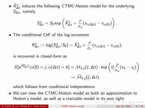
Xα∆t induces the following CTMC-Heston model for the underlying

S∆t , namely

Sα∆t = S0 exp

(Xα

∆t +ρ

σv(vα(∆t) − vα(0))

).

The conditional ChF of the log-increment

Rα∆t := log(Sα∆t/S0) = Xα∆t +

ρ

σv(vα(∆t) − vα(0)),

is recovered in closed-form as

E[e iRα∆tξ|α(0) = j , α(∆t) = k] =Mk,j(ξ; ∆t) · exp

(iξρ

σv(vk − vj)

):= Mk,j(ξ; ∆t).

which follows from conditional independence.

We can view the CTMC-Heston model as both an approximation toHeston’s model, as well as a tractable model in its own right.


Calibration of the CTMC-Heston model

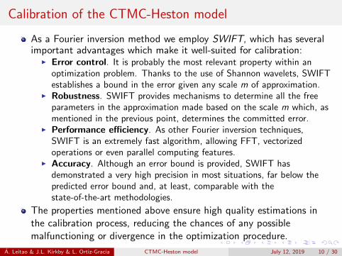
As a Fourier inversion method we employ SWIFT, which has severalimportant advantages which make it well-suited for calibration:

I Error control. It is probably the most relevant property within anoptimization problem. Thanks to the use of Shannon wavelets, SWIFTestablishes a bound in the error given any scale m of approximation.

I Robustness. SWIFT provides mechanisms to determine all the freeparameters in the approximation made based on the scale m which, asmentioned in the previous point, determines the committed error.

I Performance efficiency. As other Fourier inversion techniques,SWIFT is an extremely fast algorithm, allowing FFT, vectorizedoperations or even parallel computing features.

I Accuracy. Although an error bound is provided, SWIFT hasdemonstrated a very high precision in most situations, far below thepredicted error bound and, at least, comparable with thestate-of-the-art methodologies.

The properties mentioned above ensure high quality estimations inthe calibration process, reducing the chances of any possiblemalfunctioning or divergence in the optimization procedure.


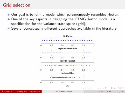
Grid selection

Our goal is to form a model which parsimoniously resembles Heston.One of the key aspects in designing the CTMC-Heston model is aspecification for the variance state-space (grid).Several conceptually different approaches available in the literature.

0 0.2 0.4 0.6 0.8 1

Uniform

0 0.2 0.4 0.6 0.8 1

Mijatovic-Pistorius

0 0.2 0.4 0.6 0.8 1

Tavella-Randall

0 0.2 0.4 0.6 0.8 1

Lo-Skindilias


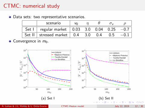
CTMC: numerical study

Data sets: two representative scenarios.

scenario v0 η θ σv ρ

Set I regular market 0.03 3.0 0.04 0.25 −0.7

Set II stressed market 0.4 3.0 0.4 0.5 −0.1

Convergence in m0.

50 100 150 20010-6

10-5

10-4

10-3

10-2

10-1

UniformMijatovic-PistoriusTavella-RandallLo-Skindilias

(a) Set I

50 100 150 20010-8

10-7

10-6

10-5

10-4

10-3


(b) Set II

Figure: Market parameters: put option, S0 = 100, K = 100, r = 0.05 and T = 1.A. Leitao & J.L. Kirkby & L. Ortiz-Gracia CTMC-Heston model July 12, 2019 12 / 30

Influence of the model parameters

0.05 0.1 0.15 0.2

10-6

10-4

10-2

100


0.05 0.1 0.15 0.2

10-6

10-4

10-2


1 2 3 4 510-6

10-5

10-4

10-3

10-2


0.2 0.4 0.6 0.8 110-10

10-8

10-6

10-4

10-2

100


-1 -0.5 0 0.5 1

10-8

10-6

10-4

10-2UniformMijatovic-PistoriusTavella-RandallLo-Skindilias

2 4 6 8 1010-6

10-5

10-4

10-3

10-2


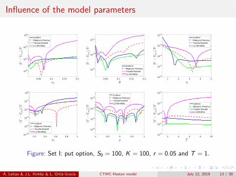
Figure: Set I: put option, S0 = 100, K = 100, r = 0.05 and T = 1.


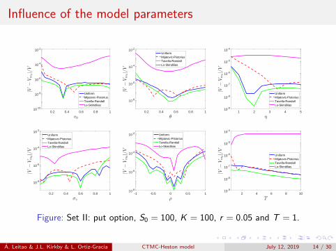
Influence of the model parameters

0.2 0.4 0.6 0.8 110-10

10-8

10-6

10-4

10-2


0.2 0.4 0.6 0.8 1

10-8

10-6

10-4

10-2


1 2 3 4 510-9

10-8

10-7

10-6

10-5

10-4


0.2 0.4 0.6 0.8 1

10-8

10-6

10-4

10-2


-1 -0.5 0 0.5 110-8

10-6

10-4

10-2 UniformMijatovic-PistoriusTavella-RandallLo-Skindilias

2 4 6 8 1010-9

10-8

10-7

10-6

10-5

10-4


Figure: Set II: put option, S0 = 100, K = 100, r = 0.05 and T = 1.


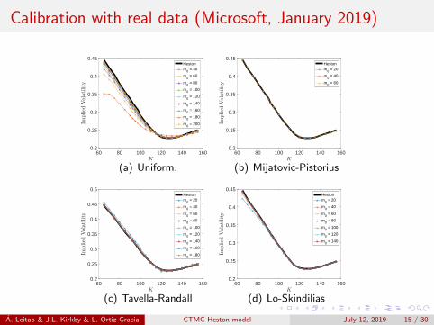
Calibration with real data (Microsoft, January 2019)

60 80 100 120 140 1600.2

0.25

0.3

0.35

0.4

0.45Hestonm

0 = 40

m0 = 60

m0 = 80

m0 = 100

m0 = 120

m0 = 140

m0 = 160

m0 = 180

m0 = 200

(a) Uniform.

60 80 100 120 140 1600.2

0.25

0.3

0.35

0.4

0.45Hestonm

0 = 20

m0 = 40

m0 = 60

(b) Mijatovic-Pistorius

60 80 100 120 140 1600.2

0.25

0.3

0.35

0.4

0.45

0.5Hestonm

0 = 20

m0 = 40

m0 = 60

m0 = 80

m0 = 100

m0 = 120

m0 = 140

m0 = 160

m0 = 180

(c) Tavella-Randall

60 80 100 120 140 1600.2

0.25

0.3

0.35

0.4

0.45Hestonm

0 = 20

m0 = 40

m0 = 60

m0 = 80

m0 = 100

m0 = 120

m0 = 140

(d) Lo-Skindilias

Figure: Microsoft calibration curves for varying m0. Market parameters: calloptions, S0 = 105.36, K = {65, 70, . . . , 150, 155}, r = 0.0246 and T = 0.4986.Heston parameters:v0 = 0.0906, η = 0.8549, θ = 0.1379, σv = 0.9976, ρ = −0.6187.


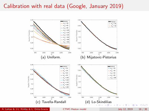
Calibration with real data (Google, January 2019)

900 1000 1100 1200 1300

0.26

0.28

0.3

0.32

0.34

0.36Hestonm

0 = 40

m0 = 60

m0 = 80

m0 = 100

m0 = 120

m0 = 140

m0 = 160

m0 = 180

m0 = 200

(a) Uniform.

900 1000 1100 1200 1300

0.26

0.28

0.3

0.32

0.34

0.36Hestonm

0 = 20

m0 = 40

(b) Mijatovic-Pistorius

900 1000 1100 1200 1300

0.26

0.28

0.3

0.32

0.34

0.36

0.38Hestonm

0 = 20

m0 = 40

m0 = 60

m0 = 80

m0 = 100

m0 = 120

m0 = 140

m0 = 160

m0 = 180

(c) Tavella-Randall

900 1000 1100 1200 1300

0.26

0.28

0.3

0.32

0.34

0.36Hestonm

0 = 20

m0 = 40

m0 = 60

m0 = 80

m0 = 100

(d) Lo-Skindilias

Figure: Google implied volatility: call options, S0 = 1080.66,K = {880, 890, . . . , 1390, 1395}, r = 0.0249 and T = 0.9972;v0 = 0.1482, η = 0.7752, θ = 0.0722, σv = 0.9278, ρ = −0.5444.


Interesting lessons

All the approaches provide numerical convergence in m0.

The error decays very fast at the beginning, with smaller m0, andsmoothens for bigger m0, suggesting a damping effect.

The grid distribution proposed by Lo and Skindilias provides, ingeneral, poorer estimations.

Although the uniform approach performs surprisingly well in the testwith synthetic parameters, the real calibration experiment shows apretty inaccurate estimations for options far from at-the-money strike.

The schemes by Mijatovic-Pistorius and Tavella-Randall performsimilarly. It is worth noting that the first explodes when the initial andlong-term volatilities differ greatly one from the other. The secondhappens to be the most robust and precise choice in general.

By focusing on the correlation parameter, ρ, in the second test, weobserve that the error tends to be minimum close to the no-correlationpoint (ρ = 0), and it degrades when ρ ventures far form zero.


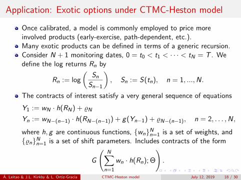
Application: Exotic options under CTMC-Heston model

Once calibrated, a model is commonly employed to price moreinvolved products (early-exercise, path-dependent, etc.).Many exotic products can be defined in terms of a generic recursion.Consider N + 1 monitoring dates, 0 = t0 < t1 < · · · < tN = T . Wedefine the log returns Rn by

Rn := log

(SnSn−1

), Sn := S(tn), n = 1, ...,N.

The contracts of interest satisfy a very general sequence of equations

Y1 := wN · h(RN) + %N

Yn := wN−(n−1) · h(RN−(n−1)) + g(Yn−1) + %N−(n−1), n = 2, . . . ,N,

where h, g are continuous functions, {wn}Nn=1 is a set of weights, and{%n}Nn=1 is a set of shift parameters. Includes contracts of the form

G

(N∑

n=1

wn · h(Rn); Θ

).


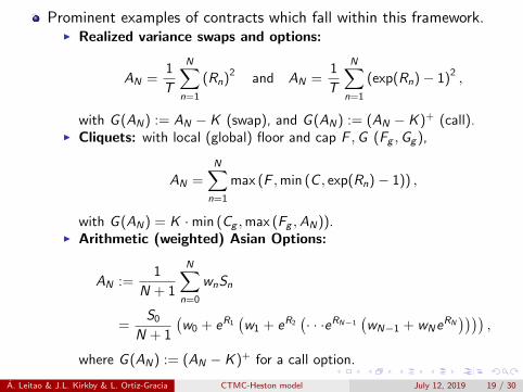
Prominent examples of contracts which fall within this framework.I Realized variance swaps and options:

AN =1

T

N∑n=1

(Rn)2 and AN =1

T

N∑n=1

(exp(Rn)− 1)2,

with G (AN) := AN − K (swap), and G (AN) := (AN − K )+ (call).I Cliquets: with local (global) floor and cap F ,G (Fg ,Gg ),

AN =N∑

n=1

max (F ,min (C , exp(Rn)− 1)) ,

with G (AN) = K ·min (Cg ,max (Fg ,AN)).I Arithmetic (weighted) Asian Options:

AN :=1

N + 1

N∑n=0

wnSn

=S0

N + 1

(w0 + eR1

(w1 + eR2

(· · ·eRN−1

(wN−1 + wNe

RN))))

,

where G (AN) := (AN − K )+ for a call option.


Numerical experiments with exotic options

We will present some experiments aiming to numerically validate theintroduced CTMC-Heston model.

We will consider several exotic contracts: realized variance swaps,realized variance options and Asian options.

The recursive definition above allows efficient Fourier methods(SWIFT).

The realized variance swaps are chosen for comparative purposes,since an exact solution for the Heston model is available.

That is not the case for the other two products, which often requirethe use of MC methods.

Computer system CPU Intel Core i7-4720HQ 2.6GHz, 16GB RAMand Matlab R2017b.

Based on the calibration tests, Tavella-Randall scheme is used.

MC setting: QE scheme with 106 paths and 360 time steps.


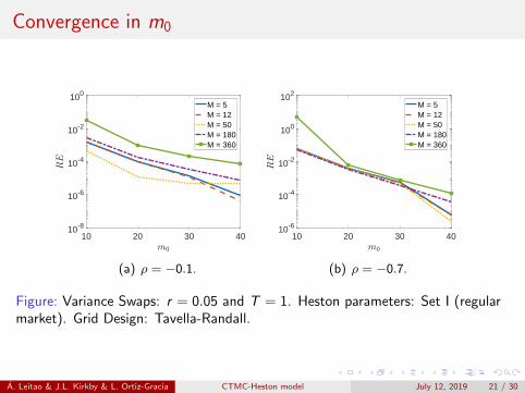
Convergence in m0

10 20 30 4010-8

10-6

10-4

10-2

100

M = 5M = 12M = 50M = 180M = 360

(a) ρ = −0.1.

10 20 30 4010-6

10-4

10-2

100

102

M = 5M = 12M = 50M = 180M = 360

(b) ρ = −0.7.

Figure: Variance Swaps: r = 0.05 and T = 1. Heston parameters: Set I (regularmarket). Grid Design: Tavella-Randall.


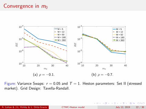
Convergence in m0

10 20 30 4010-7

10-6

10-5

10-4

M = 5M = 12M = 50M = 180M = 360

(a) ρ = −0.1.

10 20 30 4010-6

10-5

10-4

10-3

M = 5M = 12M = 50M = 180M = 360

(b) ρ = −0.7.

Figure: Variance Swaps: r = 0.05 and T = 1. Heston parameters: Set II (stressedmarket). Grid Design: Tavella-Randall.


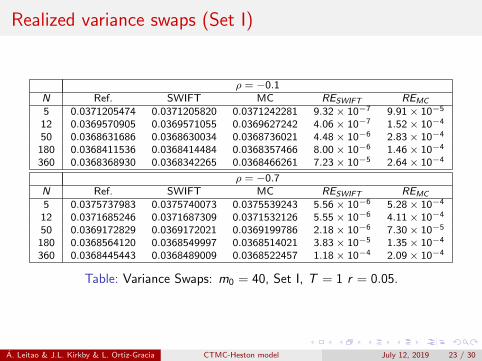
Realized variance swaps (Set I)

ρ = −0.1N Ref. SWIFT MC RESWIFT REMC

5 0.0371205474 0.0371205820 0.0371242281 9.32× 10−7 9.91× 10−5

12 0.0369570905 0.0369571055 0.0369627242 4.06× 10−7 1.52× 10−4

50 0.0368631686 0.0368630034 0.0368736021 4.48× 10−6 2.83× 10−4

180 0.0368411536 0.0368414484 0.0368357466 8.00× 10−6 1.46× 10−4

360 0.0368368930 0.0368342265 0.0368466261 7.23× 10−5 2.64× 10−4


5 0.0375737983 0.0375740073 0.0375539243 5.56× 10−6 5.28× 10−4

12 0.0371685246 0.0371687309 0.0371532126 5.55× 10−6 4.11× 10−4

50 0.0369172829 0.0369172021 0.0369199786 2.18× 10−6 7.30× 10−5

180 0.0368564120 0.0368549997 0.0368514021 3.83× 10−5 1.35× 10−4

360 0.0368445443 0.0368489009 0.0368522457 1.18× 10−4 2.09× 10−4

Table: Variance Swaps: m0 = 40, Set I, T = 1 r = 0.05.


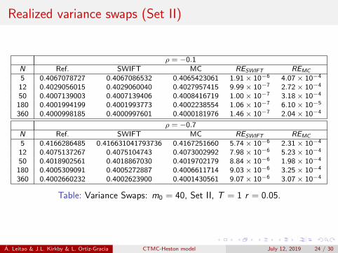
Realized variance swaps (Set II)


5 0.4067078727 0.4067086532 0.4065423061 1.91× 10−6 4.07× 10−4

12 0.4029056015 0.4029060040 0.4027957415 9.99× 10−7 2.72× 10−4

50 0.4007139003 0.4007139406 0.4008416719 1.00× 10−7 3.18× 10−4

180 0.4001994199 0.4001993773 0.4002238554 1.06× 10−7 6.10× 10−5

360 0.4000998185 0.4000997601 0.4000181976 1.46× 10−7 2.04× 10−4


5 0.4166286485 0.416631041793736 0.4167251660 5.74× 10−6 2.31× 10−4

12 0.4075137267 0.4075104743 0.4073002992 7.98× 10−6 5.23× 10−4

50 0.4018902561 0.4018867030 0.4019702179 8.84× 10−6 1.98× 10−4

180 0.4005309091 0.4005272887 0.4006611714 9.03× 10−6 3.25× 10−4

360 0.4002660232 0.4002623900 0.4001430561 9.07× 10−6 3.07× 10−4

Table: Variance Swaps: m0 = 40, Set II, T = 1 r = 0.05.


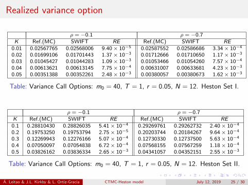
Realized variance option

ρ = −0.1 ρ = −0.7K Ref.(MC) SWIFT RE Ref.(MC) SWIFT RE

0.01 0.02567765 0.02568006 9.40× 10−5 0.02587552 0.02586686 3.34× 10−4

0.02 0.01699106 0.01701443 1.37× 10−3 0.01712666 0.01710650 1.17× 10−3

0.03 0.01045427 0.01044283 1.09× 10−3 0.01053466 0.01054260 7.57× 10−4

0.04 0.00613621 0.00613145 7.75× 10−4 0.00631007 0.00633681 4.23× 10−3

0.05 0.00351388 0.00352261 2.48× 10−3 0.00380057 0.00380673 1.62× 10−3

Table: Variance Call Options: m0 = 40, T = 1, r = 0.05, N = 12. Heston Set I.

ρ = −0.1 ρ = −0.7K Ref.(MC) SWIFT RE Ref.(MC) SWIFT RE0.1 0.28810430 0.28826035 5.41× 10−4 0.29269761 0.29262732 2.40× 10−4

0.2 0.19753250 0.19753794 2.75× 10−5 0.20203744 0.20184267 9.64× 10−4

0.3 0.12269943 0.12276166 5.07× 10−4 0.12730330 0.12737500 5.63× 10−4

0.4 0.07050097 0.07054838 6.72× 10−4 0.07568155 0.07567259 1.18× 10−4

0.5 0.03826162 0.03836334 2.65× 10−3 0.04341057 0.04352151 2.55× 10−3

Table: Variance Call Options: m0 = 40, T = 1, r = 0.05, N = 12. Heston Set II.


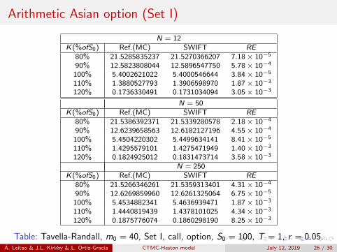
Arithmetic Asian option (Set I)

N = 12K(%ofS0) Ref.(MC) SWIFT RE

80% 21.5285835237 21.5270366207 7.18× 10−5

90% 12.5823808044 12.5896547750 5.78× 10−4

100% 5.4002621022 5.4000546644 3.84× 10−5

110% 1.3880527793 1.3906598970 1.87× 10−3

120% 0.1736330491 0.1731034094 3.05× 10−3


80% 21.5386392371 21.5339280578 2.18× 10−4

90% 12.6239658563 12.6182127196 4.55× 10−4

100% 5.4504220302 5.4499634141 8.41× 10−5

110% 1.4295579101 1.4275471949 1.40× 10−3

120% 0.1824925012 0.1831473714 3.58× 10−3


80% 21.5266346261 21.5359313401 4.31× 10−4

90% 12.6269859960 12.6261325064 6.75× 10−5

100% 5.4534882341 5.4636939471 1.87× 10−3

110% 1.4440819439 1.4378101025 4.34× 10−3

120% 0.1875776074 0.1860298190 8.25× 10−3

Table: Tavella-Randall, m0 = 40, Set I, call, option, S0 = 100, T = 1, r = 0.05.A. Leitao & J.L. Kirkby & L. Ortiz-Gracia CTMC-Heston model July 12, 2019 26 / 30

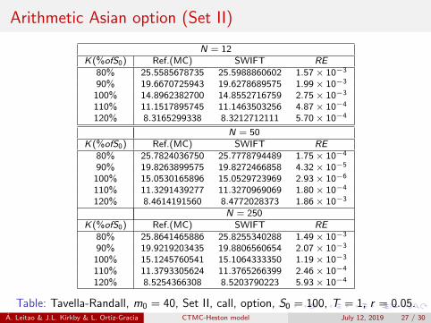
Arithmetic Asian option (Set II)


80% 25.5585678735 25.5988860602 1.57× 10−3

90% 19.6670725943 19.6278689575 1.99× 10−3

100% 14.8962382700 14.8552716759 2.75× 10−3

110% 11.1517895745 11.1463503256 4.87× 10−4

120% 8.3165299338 8.3212712111 5.70× 10−4


80% 25.7824036750 25.7778794489 1.75× 10−4

90% 19.8263899575 19.8272466858 4.32× 10−5

100% 15.0530165896 15.0529723969 2.93× 10−6

110% 11.3291439277 11.3270969069 1.80× 10−4

120% 8.4614191560 8.4772028373 1.86× 10−3


80% 25.8641465886 25.8255340288 1.49× 10−3

90% 19.9219203435 19.8806560654 2.07× 10−3

100% 15.1245760541 15.1064333350 1.19× 10−3

110% 11.3793305624 11.3765266399 2.46× 10−4

120% 8.5254366308 8.5203790223 5.93× 10−4

Table: Tavella-Randall, m0 = 40, Set II, call, option, S0 = 100, T = 1, r = 0.05.A. Leitao & J.L. Kirkby & L. Ortiz-Gracia CTMC-Heston model July 12, 2019 27 / 30

Conclusions

This work provides a general, computationally efficient, and robustvaluation framework under the CTMC-Heston model.

This model approximation provides a parsimonious and faithfulrepresentation of the Heston model, and it is able to reproduce thesame volatility smile structure with a modest number of states.

We can efficiently price a large variety of contracts which areexceptionally difficult to handle under Heston’s model.

The efficiency of the method is obtained by combining the CTMCapproximation of the variance, with the SWIFT Fourier method.

An extensive set of numerical experiments were provided, analyzingAsian options and discretely sampled realized variance derivatives.

A detailed error analysis will follow (work in progress).


References

Zhenyu Cui, Justin L. Kirkby, and Duy Nguyen.Springer IMA volume: Recent Developments in Financial and Economic Applications,chapter Continuous-Time Markov Chain and Regime Switching approximations withapplications to options pricing.Forthcoming, Springer, 2019.

Alvaro Leitao, Luis Ortiz-Gracia, and Emma I. Wagner.SWIFT valuation of discretely monitored arithmetic Asian options.Journal of Computational Science, 28:120–139, 2018.

Chia Chun Lo and Konstantinos Skindilias.An improved Markov chain approximation methodology: derivatives pricing and modelcalibration.International Journal of Theoretical and Applied Finance, 17(07):1450047, 2014.

Aleksandar Mijatovic and Martijn Pistorius.Continuously monitored barrier options under Markov processes.Mathematical Finance, 23(1):1–38, 2013.

Domingo Tavella and Curt Randall.Pricing Financial Instruments: The Finite Difference Method.Wiley, 2000.


Acknowledgements & Questions

Thanks to support from MDM-2014-0445

More: alvaroleitao.github.io

Thank you for your attentionA. Leitao & J.L. Kirkby & L. Ortiz-Gracia CTMC-Heston model July 12, 2019 30 / 30

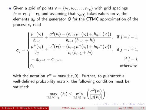
Given a grid of points v = {v1, v2, . . . , vm0} with grid spacingshi = vi+1 − vi , and assuming that vα(t) takes values on v, theelements qij of the generator Q for the CTMC approximation of theprocess vt read

qij =

µ−(vi )

hi−1+σ2(vi )− (hi−1µ

−(vi ) + hiµ+(vi ))

hi−1 (hi−1 + hi ), if j = i − 1,

µ+(vi )

hi+σ2(vi )− (hi−1µ

−(vi ) + hiµ+(vi ))

hi (hi−1 + hi ), if j = i + 1,

− qi ,i−1 − qi ,i+1, if j = i ,

0, otherwise,

with the notation z± = max(±z , 0). Further, to guarantee awell-defined probability matrix, the following condition must besatisfied:

max1≤i<m0

(hi ) ≤ min1≤i≤m0

(σ2(vi )

|µ(vi )|

).



Documents

Continuous Time Markov Chain approximation of the Heston model · Time Markov Chain (CTMC) approximation to the variance process. The new formulation enables a closed-form solution