Continuous-time ﬁlters - Veřejné služby … RPU/XXX P2: RPU/XXX QC: RPU/XXX T1: RPU CUUK852-Mandal & Asif November 17, 2006 16:7 324 Part II Continuous-time signals and systems

P1: RPU/XXX P2: RPU/XXX QC: RPU/XXX T1: RPU

CUUK852-Mandal & Asif November 17, 2006 16:7

C H A P T E R

7 Continuous-time filters

A common requirement in signal processing is to modify the frequency contentsof a continuous-time (CT) signal in a predefined manner. In communication sys-tems, for example, noise and interference from the neighboring channels cor-rupt the information-bearing signal transmitted via a communication channel,such as a telephone line. By exploiting the differences between the frequencycharacteristics of the transmitted signal and the channel noise, a linear time-invariant system (LTI) system can be designed to compensate for the distortionintroduced during the transmission. Such an LTI system is referred to as afrequency-selective filter, which processes the received signal to eliminate thehigh-frequency components introduced by the channel interference and noisefrom the low-frequency components constituting the information-bearing sig-nal. The range of frequencies eliminated from the CT signal applied at the inputof the filter is referred to as the stop band of the filter, while the range of fre-quencies that is left relatively unaffected by the filter constitute the pass bandof the filter.

Graphic equalizers used in stereo sound systems provide another applicationfor the continuous-time (CT) filters. A graphic equalizer consists of a combina-tion of CT filters, each tuned to a different band of frequencies. By selectivelyamplifying or attenuating the frequencies within the operational bands of theconstituent filters, a graphic equalizer maintains sound consistency within dis-similar acoustic environments and spaces. The operation of a graphic equalizeris somewhat different from that of a frequency-selective filter used in our earlierexample of the communication system since it amplifies or attenuates selectedfrequency components of the input signal. A frequency-selective filter, on theother hand, attempts to eliminate the frequency components completely withinthe stop band of the filter.

This chapter focuses on the design of CT filters. We are particularly interestedin the frequency-selective filters that are categorized in four different categories(lowpass, highpass, bandpass, and bandstop) in Section 7.1. Practical approxi-mations to the frequency characteristics of the ideal frequency-selective filtersare presented in Section 7.2, where acceptable levels of distortion is tolerated

320



321 7 Continuous-time filters

within the pass and stop bands of the ideal filters. Section 7.3 designs threerealizable implementations of an ideal lowpass filter. These implementationsare referred to as the Butterworth, Chebyshev, and elliptic filters. Section 7.4transforms the frequency characteristics of the highpass, bandpass, and band-stop filters in terms of the characteristics of the lowpass filters. These transfor-mations are exploited to design the highpass, bandpass, and bandstop filters.Finally, the chapter is concluded with a summary of important concepts inSection 7.5.

7.1 Filter classification

An ideal frequency-selective filter is a system that passes a prespecified rangeof frequency components without any attenuation but completely rejects theremaining frequency components. As discussed earlier, the range of input fre-quencies that is left unaffected by the filter is referred to as the pass band of thefilter, while the range of input frequencies that are blocked from the output isreferred to as the stop band of the filter. In terms of the magnitude spectrum, theabsolute value of the transfer function |H (�)| of the frequency filter, therefore,toggles between the values of A and zero as a function of frequency �. Thegain |H (�)| is A, typically set to one, within the pass band, while |H (�)| iszero within the stop band. Depending upon the range of frequencies within thepass and stop bands, an ideal frequency-selective filter is categorized in fourdifferent categories. These categories are defined in the following.

7.1.1 Lowpass filters

The transfer function Hlp(�) of an ideal lowpass filter is defined as follows:

Hlp(�) ={

A |�| ≤ �c

0 |�| > �c,(7.1)

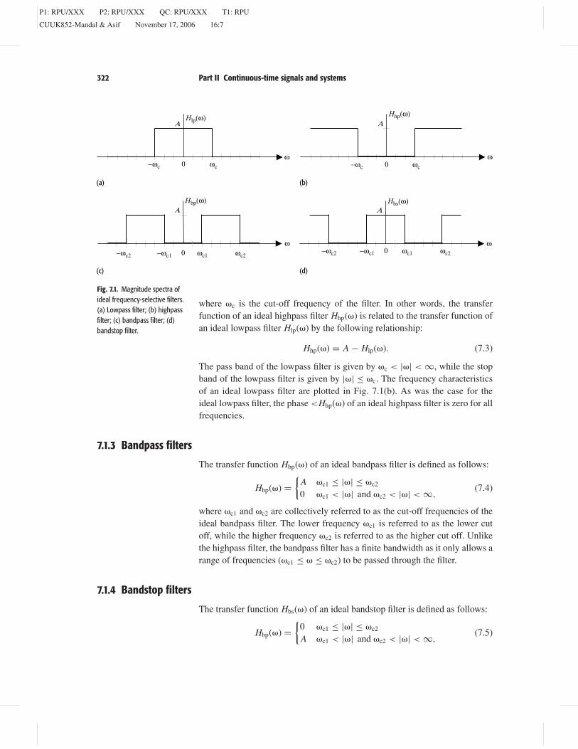
where �c is referred to as the cut-off frequency of the filter. The pass band ofthe lowpass filter is given by |�| ≤ �c, while the stop band of the lowpass filteris given by �c < |�| < ∞. The frequency characteristics of an ideal lowpassfilter are plotted in Fig. 7.1(a), where we observe that the magnitude |Hlp(�)|toggles between the values of A within the pass band and zero within the stopband. The phase <Hlp(�) of an ideal lowpass filter is zero for all frequencies.

7.1.2 Highpass filters

The transfer function Hhp(�) of an ideal highpass filter is defined as follows:

Hhp(�) ={

0 |�| ≤ �c

A |�| > �c,(7.2)



322 Part II Continuous-time signals and systems

ω0

ΑHlp(ω)

ωc−ωc 0 ωc−ωc

ω0

ΑHbp(ω)

−ωc2 −ωc1 ωc1 ωc20−ωc2 −ωc1 ωc1 ωc2

ω

ΑHbs(ω)

ω

ΑHhp(ω)

(a) (b)

(c) (d)

Fig. 7.1. Magnitude spectra ofideal frequency-selective filters.(a) Lowpass filter; (b) highpassfilter; (c) bandpass filter; (d)bandstop filter.

where �c is the cut-off frequency of the filter. In other words, the transferfunction of an ideal highpass filter Hhp(�) is related to the transfer function ofan ideal lowpass filter Hlp(�) by the following relationship:

Hhp(�) = A − Hlp(�). (7.3)

The pass band of the lowpass filter is given by �c < |�| < ∞, while the stopband of the lowpass filter is given by |�| ≤ �c. The frequency characteristicsof an ideal lowpass filter are plotted in Fig. 7.1(b). As was the case for theideal lowpass filter, the phase <Hhp(�) of an ideal highpass filter is zero for allfrequencies.

7.1.3 Bandpass filters

The transfer function Hbp(�) of an ideal bandpass filter is defined as follows:

Hbp(�) ={

A �c1 ≤ |�| ≤ �c2

0 �c1 < |�| and �c2 < |�| < ∞,(7.4)

where �c1 and �c2 are collectively referred to as the cut-off frequencies of theideal bandpass filter. The lower frequency �c1 is referred to as the lower cutoff, while the higher frequency �c2 is referred to as the higher cut off. Unlikethe highpass filter, the bandpass filter has a finite bandwidth as it only allows arange of frequencies (�c1 ≤ � ≤ �c2) to be passed through the filter.

7.1.4 Bandstop filters

The transfer function Hbs(�) of an ideal bandstop filter is defined as follows:

Hbp(�) ={

0 �c1 ≤ |�| ≤ �c2

A �c1 < |�| and �c2 < |�| < ∞,(7.5)




where �c1 and �c2 are, respectively, referred to as the lower cut-off and highercut-off frequencies of the ideal bandstop filter. A bandstop filter can be imple-mented from a bandpass filter using the following relationship:

Hbs(�) = A − Hbp(�). (7.6)

The ideal bandstop filter is the converse of the ideal bandpass filter as it elimi-nates a certain range of frequencies (�c1 ≤ � ≤ �c2) from the input signal.

In the above discussion, we used the transfer function to categorize differenttypes of frequency selective filters. Example 7.1 derives the impulse responsefor ideal lowpass and highpass filters.

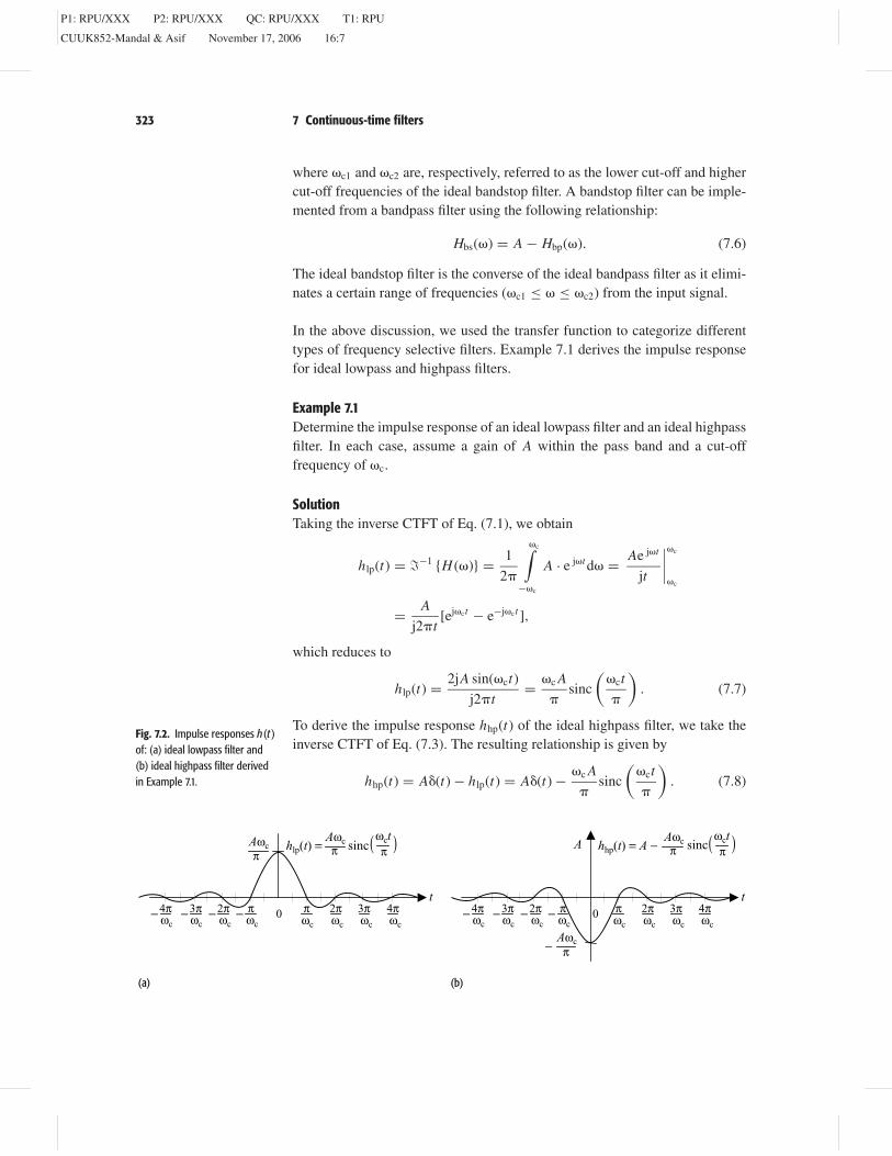
Example 7.1Determine the impulse response of an ideal lowpass filter and an ideal highpassfilter. In each case, assume a gain of A within the pass band and a cut-offfrequency of �c.

SolutionTaking the inverse CTFT of Eq. (7.1), we obtain

hlp(t) = �−1 {H (�)} = 1

2�

�c∫−�c

A · e j�t d� = Ae j�t

jt

∣∣∣∣�c

�c

= A

j2�t[ej�ct − e−j�ct ],

which reduces to

hlp(t) = 2jA sin(�ct)

j2�t= �c A

�sinc

(�ct

�

). (7.7)

To derive the impulse response hhp(t) of the ideal highpass filter, we take theinverse CTFT of Eq. (7.3). The resulting relationship is given by

hhp(t) = A�(t) − hlp(t) = A�(t) − �c A

�sinc

(�ct

�

). (7.8)

0

t

( )ωctππhlp(t) = sinc

ωc−4π

ωc−3π

ωc− π

ωc−2π

ωc

4πωc

3πωc

π

πAωc

Aωc

ωc

2π 0

t

( )ωctππhhp(t) = A −

ωc−4π

ωc−3π

ωc−

−

πωc

−2πωc

4πωc

3πωc

π

πAωc

AωcA

ωc

2π

(a) (b)

sinc

Fig. 7.2. Impulse responses h(t )of: (a) ideal lowpass filter and(b) ideal highpass filter derivedin Example 7.1.




The impulse responses of ideal lowpass and highpass filters are plotted inFig. 7.2. In both cases, we note that the filters have an infinite length in thetime domain. Also, both filters are non-causal since h(t) �= 0 for t < 0.

7.2 Non-ideal filter characteristics

As is true for any ideal system, the ideal frequency-selective filters are notphysically realizable for a variety of reasons. From the frequency characteristicsof the ideal filters, we note that the gain A of the filters is constant within thepass band, while the gain within the stop band is strictly zero. A second issuewith the transfer functions H (�), specified for ideal filters in Eqs (7.1)–(7.5),is the sharp transition between the pass and stop bands such that there is adiscontinuity in H (�) at � = �c. In practice, we cannot implement filters withconstant gains within the pass and stop bands. Also, abrupt transitions cannotbe designed. This is observed in Example 7.1, where the constant gains andthe sharp transition in the ideal lowpass and highpass filters lead to non-causalimpulse responses which are of infinite length. Clearly, such LTI systems cannotbe implemented in the physical world.

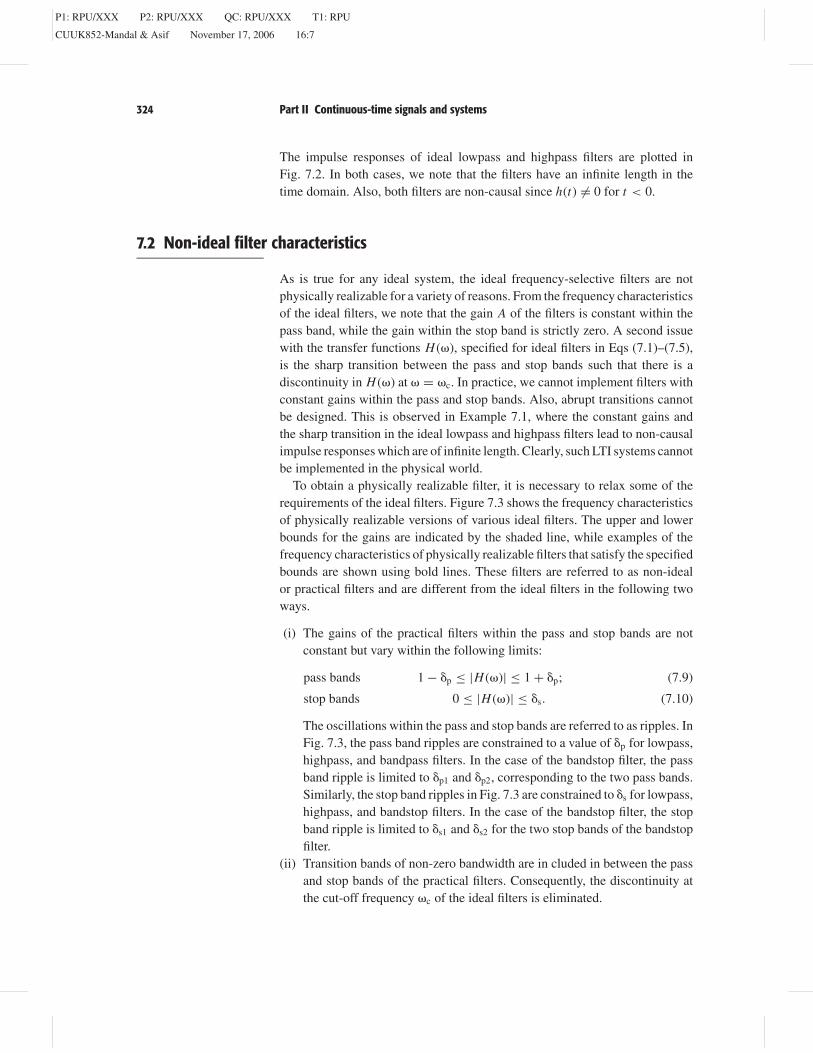
To obtain a physically realizable filter, it is necessary to relax some of therequirements of the ideal filters. Figure 7.3 shows the frequency characteristicsof physically realizable versions of various ideal filters. The upper and lowerbounds for the gains are indicated by the shaded line, while examples of thefrequency characteristics of physically realizable filters that satisfy the specifiedbounds are shown using bold lines. These filters are referred to as non-idealor practical filters and are different from the ideal filters in the following twoways.

(i) The gains of the practical filters within the pass and stop bands are notconstant but vary within the following limits:

pass bands 1 − �p ≤ |H (�)| ≤ 1 + �p; (7.9)

stop bands 0 ≤ |H (�)| ≤ �s. (7.10)

The oscillations within the pass and stop bands are referred to as ripples. InFig. 7.3, the pass band ripples are constrained to a value of �p for lowpass,highpass, and bandpass filters. In the case of the bandstop filter, the passband ripple is limited to �p1 and �p2, corresponding to the two pass bands.Similarly, the stop band ripples in Fig. 7.3 are constrained to �s for lowpass,highpass, and bandstop filters. In the case of the bandstop filter, the stopband ripple is limited to �s1 and �s2 for the two stop bands of the bandstopfilter.

(ii) Transition bands of non-zero bandwidth are in cluded in between the passand stop bands of the practical filters. Consequently, the discontinuity atthe cut-off frequency �c of the ideal filters is eliminated.




Hlp(ω)

Hbp(ω)

Hhp(ω)

1−δp

1+ δp

1+δp 1+ δp1

1−δp1

1+ δp2

1−δp21+δp

1−δp

1+ δp

pass band stop bandtransitionband

ω0

δs

δs2

δs1 δs

δs

ωp ωpωs ωp

stop band pass bandtransitionband

ω0

stopband I

stopband II

pass band

ω ω0

Hbs(ω)

ωs1 ωp1 ωs1 ωs2 ωp2ωp1 ωp2 ωs2

passband I

passband II

stopband

0

(a)

(c) (d)

(b)

Fig. 7.3. Frequencycharacteristics of practical filters.(a) Practical lowpass filter;(b) practical highpass filter;(c) practical bandpass filter;(d) practical bandstop filter.

Example 7.2 considers a practical lowpass filter and derives the values for thepass band and the stop band, and the associated gains of the filter.

Example 7.2Consider a practical lowpass filter with the following transfer function:

H (s) = 5.018×103s4+2.682×1014s3−1.026×104s+3.196×1024

s5+9.863×104s4+2.107×1010s3+1.376×1015s2+1.026×1020s+3.196×1024.

Assuming that the ripple �p within the pass band is limited to 1 dB and theripple �s within the stop band is limited to 40 dB, determine the pass band,transition band and stop band of the lowpass filter.

SolutionRecall that the CTFT transfer function H (�) of the lowpass filter can be obtainedby substituting s = j� in the Laplace transfer function. The resulting magnitudespectrum |H (�)| of the lowpass filter is plotted in Fig. 7.4, where Fig. 7.4(a)




0 π 2π 3π 4π 5π 6π 7π 8π3.4π0

0.5

10.8913

ω (×104)0 π 2π 3π 4π 5π 6π 7π 8π

−80−60−40−20

020

ω (×104)4.12π

(a) (b)

Fig. 7.4. Magnitude spectrum ofthe practical lowpass filter inExample 7.2 using (a) a linearscale and (b) a decibel scalealong the y-axis.

uses a linear scale for the magnitude. Figure 7.4(b) uses a decibel scale to plotthe magnitude spectrum.

Expressed on a linear scale, the pass-band ripple �p is given by 10−1/20 or0.8913. From Fig. 7.4(a), we observe that the pass-band frequency �p corre-sponding to |H (�)| = 0.8913 is given by 3.4� × 104 radians/s. Therefore, thepass band is specified by |�| ≤ 3.4� × 104 radians/s.

To determine the stop band, we use Fig. 7.4(b), which uses a decibel scale20 × log10|H (�)| to plot the magnitude spectrum. Figure 7.4(b) shows thatthe smallest frequency for which the magnitude spectrum equals a gain of40 dB is given by 4.12� × 104 radians/s. The stop band is therefore specifiedby |�| > 4.12� × 104 radians/s.

Based on the aforementioned results, it is straightforward to derive the tran-sition band as follows:

3.4� × 104 < |�| < 4.12� × 104 radians/s.

7.2.1 Cut-off frequency

An important parameter in the design of CT filters is the cut-off frequency�c of the filter, which is defined as the frequency at which the gain of thefilter drops to 0.7071 times its maximum value. Assuming a gain of unitywithin the pass band, the gain at the cut-off frequency �c is given by 0.7071 or−3 dB on a logarithmic scale. Since the cut-off frequency lies typically withinthe transitional band of the filter, for a lowpass filter

�p ≤ �c ≤ �s. (7.11)

Since the equality �p = �c = �s implies a transitional band of zero bandwidth,this equality is only valid for ideal filters.

As a side note to our discussion, we observe that in this chapter we onlyconsider positive values of frequencies � in plotting the magnitude spectrum.The majority of our designs are based on real-valued impulse responses, whichlead to frequency spectra that satisfy the Hermitian symmetry. Exploiting theeven symmetry for the magnitude spectrum, it is therefore sufficient to spec-ify the magnitude spectrum only for positive frequencies in such cases. The




pass-band, stop-band, and cut-off frequencies are also specified by positivevalues, though their counter-negative values exist for all three parameters.

Example 7.3Determine the cut-off frequency for the lowpass filter specified in Example 7.2.

SolutionBased on the magnitude spectrum, we note that the maximum gain of the filteris given by 1 or 0 dB. At the cut off frequency �c,

|H (�c)| = 0.7071 × 1 = 0.7071,

which implies that∣∣∣∣ 5.018×103( j�c)4+2.682 × 1014( j�c)2−1.026×104( j�c)+3.196 × 1024

( j�c)5+9.863×104( j�c)4+2.107×1010( j�c)3+1.376×1015( j�c)2+1.026×1020( j�c)+3.196×1024

∣∣∣∣= 0.7071.

The above equality can be solved for �c using numerical techniques inM A T L A B . The value of the cut-off frequency is given by �c = 3.462� ×104 radians/s. Note that the cut-off frequency lies within the transitionalband in between the pass and stop bands of the lowpass filter as derived inExample 7.2.

7.3 Design of CT lowpass filters

To begin our discussion of the design of CT filters, we consider a prototype ornormalized lowpass filter, defined as a lowpass filter, with a cut-off frequencyof �c = 1 radians/s. The remaining specifications for the pass and stop bandsof the normalized lowpass filter are assumed to be given by

pass band (0 ≤ |�| ≤ �p radians/s) 1 − �p ≤ |H (�)| ≤ 1 + �p; (7.12)

stop band (|�| > �s radians/s)| H (�)| ≤ �s, (7.13)

with �p ≤ �c ≤ �s. Using the transfer function of the normalized lowpass filter,it is straightforward to implement any of the more complicated CT filters.Section 7.4 considers the frequency transformations used to convert a lowpassfilter into another category of frequency-selective filters.

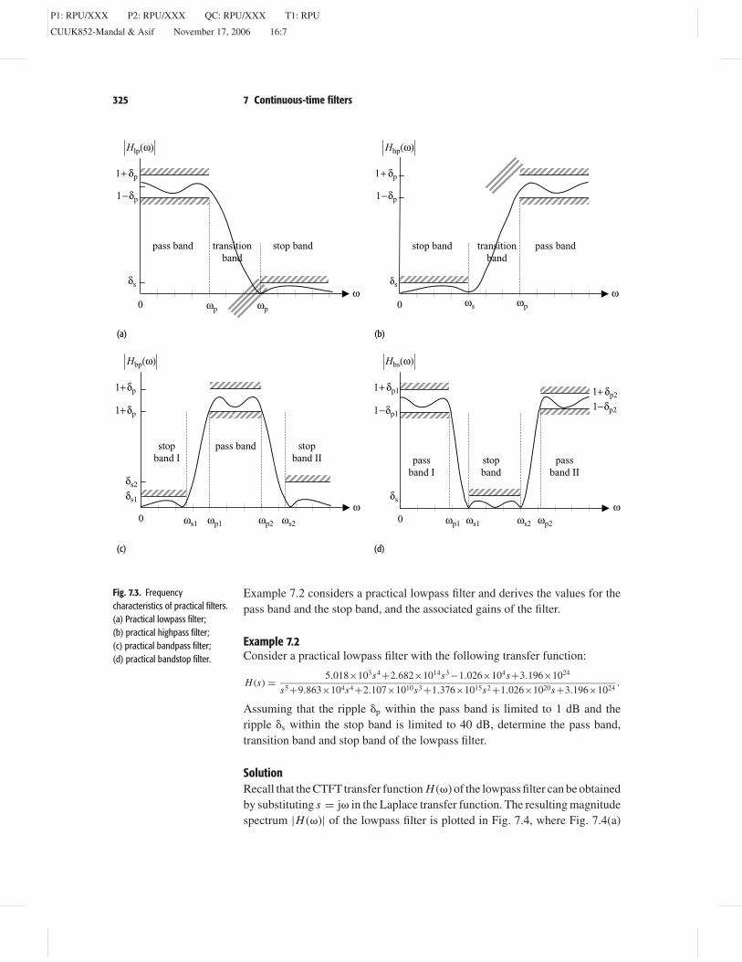
There are several specialized implementations such as Butterworth, Type IChebyshev, Type II Chebysev, and elliptic filters, which may be used to designa normalized lowpass filter. Figure 7.5 shows representative characteristics ofthese implementations, where we observe that the Butterworth filter (Fig. 7.5(a))has a monotonic transfer function such that the gain decreases monotonicallyfrom its maximum value of unity at � = 0 along the positive frequency axis.The magnitude spectrum of the Butterworth filter has negligible ripples withinthe pass and stop bands, but has a relatively lower fall off leading to a wide




transitional band. By allowing some ripples in either the pass or stop band,the Type I and Type II Chebyshev filters incorporate a sharper fall off. TheType I Chebyshev filter constitutes ripples within the pass band, while theType II Chebyshev filter allows for the stop-band ripples. Compared with theButterworth filter, both Type I and Type II Chebyshev filters have narrowertransitional bands. The elliptic filters allow for the sharpest fall off by incorpo-rating ripples in both the pass and stop bands of the filter. The elliptic filtershave the narrowest transitional band. To compare the transitional bands, Fig. 7.5plots the magnitude spectra resulting from the Butterworth, Type I Chebyshev,Type II Chebysev, and elliptic filters with the same order N .

Figure 7.5 confirms our earlier observations that the Butterworth filter(Fig. 7.5(a)) has the widest transitional band. Both the Type I and Type IIChebyshev filters (Figs 7.5(b) and (c)) have roughly equal transitional bands,which are narrower than the transitional band of the Butterworth filter. The ellip-tic filter (Fig. 7.5(d)) has the narrowest transitional band but includes ripples inboth the pass and stop bands.

We now consider the design techniques for the four specialized implemen-tations with a brief explanation of the M A T L A B library functions useful forcomputing the transfer functions of the implementations.

7.3.1 Butterworth filters

The frequency characteristics of an N th-order lowpass Butterworth filter aregiven by

|H (�)| = 1√1 +

( �

�c

)2N, (7.14)

where �c is the cut-off frequency of the filter. Substituting �c = 1 for thenormalized implementation, the transfer function of the normalized lowpassButterworth filter of order N is given by

|H (�)| = 1√1 + �2N

. (7.15)

To derive the Laplace transfer function H (s) of the normalized Butterworthfilter, we use the following relationship:

|H (�)|2 = H (s)H (−s)|s=j�. (7.16)

Substituting � = s/j, Eq. (7.16) reduces to

H (s)H (−s) = |H (s/j)|2. (7.17)




pass band stop band

pass band stop band

pass band

pass band

stop band

stop band

ω0

1+δp

δs δs

ωp

ωp ωp

ωpωs

ωs ωs

ωs

1−δp

1

1+δp

δs δs

1−δp

11+δp

1−δp

1

1+δp

1−δp

1

ω0

(a)

(c)

(b)

(d)

ω0

ω0

Fig. 7.5. Frequencycharacteristics of standardimplementations of lowpassfilters of order N . (a)Butterworth filter; (b) Type-IChebyshev filter; (c) Type-IIChebyshev filter; (d) elliptic filter.

Further substituting H (s/j) from Eq. (7.15) leads to the following expression:

H (s)H (−s) = 1

1 +( s

j

)2N , (7.18)

where the denominator represents the characteristic function for H (s)H (−s).The poles of H (s)H (−s) occur at(

s

j

)2N

= −1 = ej(2n−1)� (7.19)

or

s = j exp

[j(2n − 1)�

2N

]= exp

[j�

2+ j

(2n − 1)�

2N

](7.20)

for 0 ≤ n ≤ 2N−1. It is clear that the 2N poles for H (s)H (−s), specified inEq. (7.20), are evenly distributed along the unit circle in the complex s-plane.Of these, N poles would lie in the left half of the s-plane, while the remainingN poles would be in the right half of the s-plane. To ensure a causal and




Table 7.1. Location of the 2N poles for H (s )H (−s ) in Example 7.4 for N = 7

n 0 1 2 3 4 5 6 7 8 9 10 11 12 13pn ej3�/7 ej4�/7 ej5�/7 ej6�/7 ej� e−j6�/7 e−j5�/7 e−j4�/7 e−j3�/7 e−j2�/7 e−j�/7 1 ej�/7 ej2�/7

stable implementation, the transfer function H (s) of the normalized lowpassButterworth filter is determined from the N poles lying in the left half of thes-plane and is given by

H (s) = 1N∏

n=1

(s − pn)

, (7.21)

wherepn , for 1 ≤ n ≤ N , denotes the location of the poles in the left-halfs-plane.

Example 7.4Determine the Laplace transfer function H (s) for the normalized Butterworthfilter with cut-off frequency �c = 1 and order N = 7.

SolutionUsing Eq. (7.20), the poles of H (s)H (−s) are given by

s = exp

[j�

2+ j

(2n − 1)�

14

]

for 0 ≤ n ≤ 13. Substituting different values of n, the locations of the poles arespecified by Table 7.1. Figure 7.6 plots the locations of the poles for H (s)H (−s)in the complex s-plane. Allocating the poles located in the left-half s-plane(1 ≤ n ≤ 7), the Laplace transfer function H (s) of the Butterworth filter isgiven by

Re{s}

Im{s}

1.07π

n = 7

n = 1n = 2

n = 3n = 4

n = 5n = 6

n = 0n = 13

n = 12n = 11

n = 10n = 9

n = 8

Fig. 7.6. Location of the polesfor H (s )H (−s ) in the complexs-plane for N = 7. The poleslying in the left-half s-plane areallocated to the Butterworthfilter.

H (s) = 1

(s − ej4�/7)(s−ej5�/7)(s−ej6�/7)(s−ej�)(s−e−j6�/7)(s−e−j5�/7)(s−e−j4�/7),

which simplifies to

H (s) = 1

(s+1) [(s−ej4�/7)(s−e−j4�/7)][(s−ej5�/7)(s−e−j5�/7)][(s−ej6�/7)(s−e−j6�/7)]

or

H (s) = 1

(s + 1) (s2 + 0.4450 s + 1) (s2 + 1.2470 s + 1) (s2 + 1.8019 s + 1).

In Example 7.4, we observed that the locations of poles for the normalizedButterworth filter are complex. Since the poles occur in complex-conjugatepairs, the coefficients of the Laplace transfer function for the normalized




Table 7.2. Denominator D (s ) for transfer function H (s ) of the Butterworth filter

N D(s)

1 (s + 1)

2 (s2 + 1.414s + 1)

3 (s + 1) (s2 + s + 1)

4 (s2 + 0.7654s + 1)(s2 + 1.8478s + 1)

5 (s + 1) (s2 + 0.6810 s + 1) (s2 + 1.6810 s + 1)

6 (s2 + 0.5176s + 1)(s2 + 1.4142s + 1) (s2 + 1.9319s + 1)

7 (s + 1) (s2 + 0.4450 s + 1) (s2 + 1.2470 s + 1) (s2 + 1.8019 s + 1)

8 (s2 + 0.3902s + 1)(s2 + 1.1111s + 1) (s2 + 1.6629s + 1)(s2 + 1.9616s + 1)

9 (s + 1) (s2 + 0.3473 s + 1) (s2 + s + 1) (s2 + 1.5321 s + 1)(s2 + 1.8794 s + 1)

10 (s2 + 0.3129 s + 1) (s2 + 0.9080s + 1) (s2 + 1.4142s + 1) (s2 + 1.7820s + 1)(s2 + 1.9754 s + 1)

Butterworth filter are all real-valued. In general, Eq. (7.21) can be simplified asfollows:

H (s) = 1

D(s)= 1

s N + aN−1 s N−1 + · · · + a1 s + 1(7.22)

and represents the transfer function of the normalized Butterworth filter oforder N .

Repeating Example 7.4 for different orders (1 ≤ N ≤ 10), the transfer func-tions H (s) of the resulting normalized Butterworth filters can be similarly com-puted. Since the numerator of the transfer function is always unity, Table 7.2lists the polynomials for the denominator D(s) for 1 ≤ N ≤ 10.

7.3.1.1 Design steps for the lowpass Butterworth filter

In this section, we will design a Butterworth lowpass filter based on the spec-ifications illustrated in Fig. 7.3(a). Mathematically, the specifications can beexpressed as follows:

pass band (0 ≤ |�| ≤ �p radians/s) 1 − �p ≤ |H (�)| ≤ 1 + �p; (7.23)

stop band (|�| > �s radians/s) |H (�)| ≤ �s. (7.24)

At times, Eq. (7.23) is also expressed in terms of the pass-band ripple as20log10�p dB. Similarly, Eq. (7.24) is expressed in terms of the stop-band rippleas 20log10�s dB. The design of the Butterworth filter consists of the followingsteps, which we refer to as Algorithm 7.3.1.1.

Step 1 Determine the order N of the Butterworth filter. To determine the orderN of the filter, we calculate the gain of the filter at the corner frequencies � = �p




and � = �s. Using Eq. (7.15), the two gains are given by

pass-band corner frequency (� = �p) |H (�p)|2 = 1

1 + (�p/�c)2N= (1 − �p)2;

(7.25)

stop-band corner frequency (� = �s) |H (�s)|2 = 1

1 + (�s/�c)2N= (�s)

2.

(7.26)

Equations (7.25) and (7.26) can alternatively be expressed as follows:

(�p/�c)2N = 1

(1 − �p)2− 1 (7.27)

and

(�s/�c)2N = 1

(�s)2− 1. (7.28)

Dividing Eq. (7.27) by Eq. (7.28) and simplifying in terms of N , we obtain thefollowing expression:

N = 1

2× ln(Gp/Gs)

ln(�p/�s), (7.29)

where the gain terms are given by

Gp = 1

(1 − �p)2− 1 and Gs = 1

(�s)2− 1. (7.30)

Step 2 Using Table 7.2 or otherwise determine the transfer function for the nor-malized Butterworth filter of order N . The transfer function for the normalizedButterworth filter is denoted by H (S) with the Laplace variable S capitalizedto indicate the normalized domain.

Step 3 Determine the cut-off frequency �c of the Butterworth filter using eitherof the following two relationships:

pass-band constraint �c = �p

(Gp)1/2N; (7.31)

stop-band constraint �c = �s

(Gs)1/2N. (7.32)

If Eq. (7.31) is used to compute the cut-off frequency, then the Butterworth filterwill satisfy the pass-band constraint exactly. Similarly, the stop-band constraintwill be satisfied exactly if Eq. (7.32) is used to determine the cut-off frequency.

Step 4 Determine the transfer function H (s) of the required lowpass filterfrom the transfer function for the normalized Butterworth filter H (S), obtained




in Step 2, and the cut-off frequency �c, using the following transformation:

H (s) = H (S)|S=s/�c .

Note that the transformation S = s/�c represents scaling in the Laplace domain.It is therefore clear that the normalized cut-off frequency of 1 radian/s used inthe normalized Butterworth filter is transformed to a value of �c as required inStep 3.

Step 5 Sketch the magnitude spectrum from the transfer function H (s) deter-mined in Step 4. Confirm that the transfer function satisfies the initial designspecifications.

Examples 7.5 and 7.6 illustrate the application of the design algorithm.

Example 7.5Design a Butterworth lowpass filter with the following specifications:

pass band (0 ≤ |�| ≤ 5 radians/s) 0.8 ≤ |H (�)| ≤ 1;

stop band (|�| > 20 radians/s) |H (�)| ≤ 0.20.

SolutionUsing Step 1 of Algorithm 7.3.1.1, the gain terms Gp and Gs are given by

Gp = 1

(1 − �p)2− 1 = 1

0.82− 1 = 0.5625

and

Gs = 1

(�s)2− 1 = 1

0.22− 1 = 24.

Using Eq. (7.29), the order of the Butterworth filter is given by

N = 1

2× ln(Gp/Gs)

ln(�p/�s)= 1

2× ln(0.5625/24)

ln(5/20)= 1.3538.

We round off the order of the filter to the higher integer value as N = 2.Using Step 2 of Algorithm 7.3.1.1, the transfer function H (S) of the normal-

ized Butterworth filter with a cut-off frequency of 1 radian/s is given by

H (S) = 1

S2 + 1.414S + 1.

Using the pass-band constraint, Eq. (7.31), in Step 3 of Algorithm 7.3.1.1, thecut-off frequency of the required Butterworth filter is given by

�c = �p

(Gp)1/2N= 5

(0.5625)1/4= 5.7735 radians/s.




0 5 10 15 20 25 30 35 40 45 500

0.2

0.4

0.60.8

1

0 5 10 15 20 25 30 35 40 45 500

0.2

0.4

0.60.8

1

(a) (b)

Fig. 7.7. Magnitude spectra ofthe Butterworth lowpass filters,designed in Example 7.5, as afunction of �. Part (a) satisfiesthe constraint at the pass-bandcorner frequency, while part (b)satisfies the magnitudeconstraint at the stop-bandcorner frequency.

Using Step 4 of Algorithm 7.3.1.1, the transfer function H (s) of the requiredButterworth filter is obtained by the following transformation:

H (s) = H (S)|S=s/�c = 1

S2 + 1.414S + 1

∣∣∣∣S=s/5.7735

,

which simplifies to

H (s) = 1

(s/5.7735)2 + 1.414s/5.7735 + 1= 33.3333

s2 + 8.1637s + 33.3333.

Step 5 plots the magnitude spectrum of the Butterworth filter. The CTFT transferfunction of the Butterworth filter is given by

H (�) = H (s)|s=j� = 33.3333

(j�)2 + 8.1637(j�) + 33.3333.

The magnitude spectrum |H (�)| is plotted in Fig. 7.7(a) with the specificationsshown by the shaded lines. We observe that the design specifications are indeedsatisfied by the magnitude spectrum.

Alternative implementation An alternative implementation of the aforemen-tioned Butterworth filter can be obtained by using the stop-band constraint,Eq. (7.32), in Step 3 of Algorithm 7.3.1.1. The cut-off frequency of the alter-native implementation of the Butterworth filter is given by

�c = �s

(Gs)1/2N= 20

(24)1/4= 9.0360 radians/s.

Using Step 4 of Algorithm 7.3.1.1, the transfer function H (s) of the alternativeimplementation is obtained by the following transformation:

H (s) = H (S)|S=s/�c = 1

S2 + 1.414S + 1

∣∣∣∣S=s/9.0360

,

which simplifies to

H (s) = 1

(s/9.0360)2 + 1.414s/9.0360 + 1= 81.6497

s2 + 12.7769s + 81.6497.

Step 5 plots the magnitude spectrum of the alternative implementation of theButterworth filter in Fig. 7.7(b), which satisfies the initial design specifications.




Example 7.6Design a lowpass Butterworth filter with the following specifications:

pass band (0 ≤ |�| ≤ 50 radians/s) −1 ≤ 20 log10 |H (�)| ≤ 0;

stop band (|�| > 100 radians/s) 20 log10 |H (�)| ≤ −15.

SolutionExpressed on a linear scale, the pass-band gain is given by (1 − �p) = 10−1/20 =0.8913. Similarly, the stop-band gain is given by �s = 10−15/20 = 0.1778.

Using Step 1 of Algorithm 7.3.1.1, the gain terms Gp and Gs are given by

Gp = 1

(1 − �p)2− 1 = 1

0.89132− 1 = 0.2588

and

Gs = 1

(�s)2− 1 = 1

0.17782− 1 = 30.6327.

The order N of the Butterworth filter is obtained using Eq. (7.29) as follows:

N = 1

2× ln(Gp/Gs)

ln(�p/�s)= 1

2× ln(0.2588/30.6327)

ln(50/100)= 3.4435.

We round off the order of the filter to the higher integer value as N = 4.Using Step 2 of Algorithm 7.3.1.1, the transfer function H (S) of the normal-

ized Butterworth filter with a cut-off frequency of 1 radian/s is given by

H (S) = 1

(S2 + 0.7654S + 1)(S2 + 1.8478S + 1).

Using the pass-band constraint, Eq. (7.31), in Step 3 of Algorithm 7.3.1.1, thecut-off frequency of the required Butterworth filter is given by

�c = �p

(Gp)1/2N= 50

(0.2588)1/8= 59.2038 radians/s.

Using Step 4 of Algorithm 7.3.1.1, the transfer function H (s) of the requiredButterworth filter is obtained by the following transformation:

H (s) = H (S)|S=s/�c = 1

(S2 + 0.7654S + 1)(S2 + 1.8478S + 1)

∣∣∣∣S=s/59.2038

,

which simplifies to

H (s) = (3.5051 × 103)2

(s2 + 45.3146s + 3.5051 × 103)(s2 + 109.396s + 3.5051 × 103)

or

H (s) = 1.2286 × 107

s4 + 154.7106 s3 + 1.1976 × 104s2 + 5.4228 × 105s + 1.2286 × 107.




0 50 100 150 200 2500

0.1778

0.40.6

0.89131

0 50 100 150 200 2500

0.1778

0.40.6

0.89131

(a) (b)

Fig. 7.8. Magnitude spectra ofthe Butterworth lowpass filters,designed in Example 7.6, as afunction of �. Part (a) satisfiesthe constraint at the pass-bandcorner frequency, while part (b)satisfies the magnitudeconstraint at the stop-bandcorner frequency.

Step 5 plots the magnitude spectrum of the Butterworth filter. The CTFT transferfunction of the Butterworth filter is given by

H (�) = H (s)|s=j�

= 1.2286×107

( j�)4+154.7106 ( j�)3+1.1976×104( j�)2+5.4228×105( j�)+1.2286×107.

The magnitude spectrum |H (�)| is plotted in Fig. 7.8(a), where the labels on they-axis are chosen to correspond to the specified gains for the filter. We observethat the design specifications are satisfied by the magnitude spectrum.

Alternative implementation An alternative implementation of the aforemen-tioned Butterworth filter can be obtained by using the stop-band constraint,Eq. (7.32), in Step 3 of Algorithm 7.3.1.1. The cut-off frequency of the alter-native implementation of the Butterworth filter is given by

�c = �s

(Gs)1/2N= 100

(30.6327)1/4= 65.1969 radians/s.

Using Step 4 of Algorithm 7.3.1.1, the transfer function H (s) of the alternativeimplementation is obtained by the following transformation:

H (s) = H (S)|S=s/�c = 1

(S2 + 0.7654S + 1)(S2 + 1.8478S + 1)

∣∣∣∣S=s/65.1969

,

which simplifies to

H (s) = (4.2506 × 103)2

(s2 + 49.9017s + 4.2506 × 103)(s2 + 120.4708s + 4.2506 × 103)

or

H (s) = 1.8068 × 107

s4 + 170.3725 s3 + 1.4513 × 104s2 + 7.2419 × 105s + 1.8068 × 107 .

Step 5 plots the magnitude spectrum of the alternative implementation of theButterworth filter in Fig. 7.8(b), which satisfies the initial design specifications.

7.3.1.2 Butterworth filter design using M ATL AB

M A T L A B incorporates a number of functions to implement the design algo-rithm for the Butterworth filter specified in Section 7.3.1.1. The order N and the




cut-off wc frequency for the filter in Step 1 of Algorithm 7.3.1.1 can be deter-mined using the library function buttord, which has the following callingsyntax:

>> [N,wc] = buttord(wp,ws,Rp,Rs,‘s’);

where wp is the corner frequency of the pass band, ws is the corner frequencyof the stop band, Rp is the permissible ripple in the pass band in decibels,and Rs is the permissible attenuation in the stop band in decibels. The lastargument ‘s’ specifies that a CT filter in the Laplace domain is to be designed.In determining the cut-off frequency, M A T L A B uses the stop-band constraint,Eq. (7.32).

Having determined the order and the cut-off frequency, the coefficientsof the numerator and denominator polynomials of the Butterworth filter canbe determined using the library function butter with the following callingsyntax:

>> [num,den] = butter(N,wc,‘s’);

where num is a vector containing the coefficients of the numerator and den isa vector containing the coefficients of the denominator in decreasing powersof s.

Finally, the transfer function H (s) can be determined using the library func-tion tf as follows:

>> H = tf(num,den).

For Example 7.5, the M A T L A B commands for designing the Butterworth filterare given by

>> wp=5; ws=20; Rp=1.9382;Rs=13.9794;

% specify design parameters

% Rp = -20*log10(0.8)

= 1.9382dB

% Rs = -20*log10(0.2)

= 13.9794dB

>> [N,wc]=buttord(wp,ws,Rp,Rs,‘s’);

% determine order and cut-off

freq

>> [num,den]=butter(N,wc,‘s’);

% determine num and denom

coeff.

>> Ht = tf(num,den); % determine transfer function

>> [H,w] = freqs(num,den); % determine magnitude

spectrum

>> plot(w,abs(H)); % plot magnitude spectrum




Stepwise implementation of the above code returns the following values fordifferent variables:

Instruction II: N = 2; wc = 9.0360;

Instruction III: num = [0 0 81.6497]; den = [1.0000

12.7789 81.6497];

Instruction IV: Ht = 1/(s 2̂ + 12.78s + 81.65);

The magnitude spectrum is the same as that given in Fig. 7.7(b).

7.3.2 Type I Chebyshev filters

Butterworth filters have a relatively low roll off in the transitional band, whichleads to a large transitional bandwidth. Type I Chebyshev filters reduce thebandwidth of the transitional band by using an approximating function, referredto as the Type I Chebyshev polynomial, with a magnitude response that hasripples within the pass band. We start with the definition of the Chebyshevpolynomial.

7.3.2.1 Type I Chebyshev polynomial

The N th-order Type I Chebyshev polynomial is defined as

TN (�) ={

cos(N cos−1(�)) |�| ≤ 1cosh(N cosh−1(�)) |�| > 1,

(7.33)

where cosh(x) denotes the hyperbolic cosine function, which is given by

cosh(x) = cos( jx) = ex + e−x

2. (7.34)

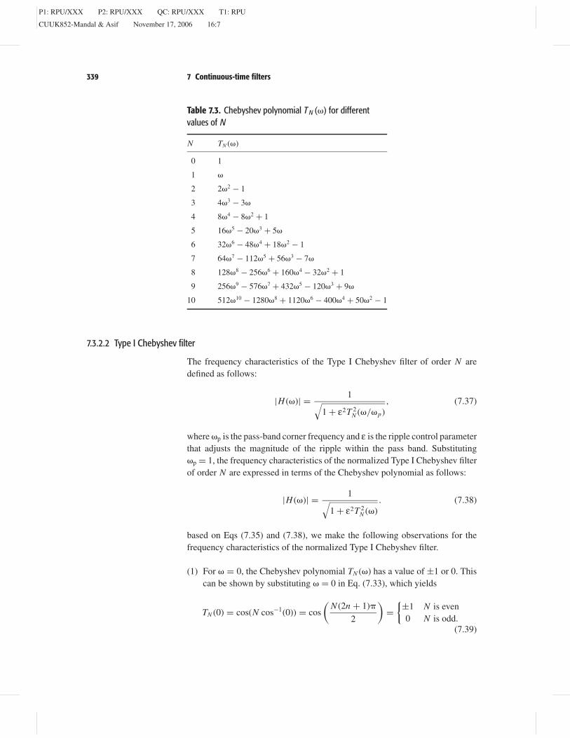
Starting from the initial values of T0(�) = 1 and T1(�) = �, the higher ordersof the Type I Chebyshev polynomial can be recursively generated using thefollowing expression:

Tn(�) = 2�Tn−1(�) − Tn−2(�). (7.35)

Table 7.3 lists the Chebyshev polynomial for different values of n within therange 0 ≤ n ≤ 10.

Using Eq. (7.33), the roots of the Type I Chebyshev polynomial TN (�) canbe derived as follows:

�n = cos

[(2n + 1)�

2N

], (7.36)

for 0 ≤ n ≤ N − 1.




Table 7.3. Chebyshev polynomial T N (�) for differentvalues of N

N TN (�)

0 1

1 �

2 2�2 − 1

3 4�3 − 3�

4 8�4 − 8�2 + 1

5 16�5 − 20�3 + 5�

6 32�6 − 48�4 + 18�2 − 1

7 64�7 − 112�5 + 56�3 − 7�

8 128�8 − 256�6 + 160�4 − 32�2 + 1

9 256�9 − 576�7 + 432�5 − 120�3 + 9�

10 512�10 − 1280�8 + 1120�6 − 400�4 + 50�2 − 1

7.3.2.2 Type I Chebyshev filter

The frequency characteristics of the Type I Chebyshev filter of order N aredefined as follows:

|H (�)| = 1√1 + ε2T 2

N (�/�p), (7.37)

where �p is the pass-band corner frequency and ε is the ripple control parameterthat adjusts the magnitude of the ripple within the pass band. Substituting�p = 1, the frequency characteristics of the normalized Type I Chebyshev filterof order N are expressed in terms of the Chebyshev polynomial as follows:

|H (�)| = 1√1 + ε2T 2

N (�). (7.38)

based on Eqs (7.35) and (7.38), we make the following observations for thefrequency characteristics of the normalized Type I Chebyshev filter.

(1) For � = 0, the Chebyshev polynomial TN (�) has a value of ±1 or 0. Thiscan be shown by substituting � = 0 in Eq. (7.33), which yields

TN (0) = cos(N cos−1(0)) = cos

(N (2n + 1)�

2

)=

{±1 N is even0 N is odd.

(7.39)




Equation (7.37) implies that the dc component |H (0)| of the Type IChebyshev filter is given by

|H (0)| =

1√1 + ε2

N is even

1 N is odd.(7.40)

(2) For � = 1 radian/s, the value of the Chebyshev polynomial TN (�) is givenby

TN (1) = cos(N cos−1(1)) = cos(2nN�) = 1. (7.41)

Therefore, the magnitude |H (�)| of the normalized Type I Chebyshev filterat � = 1 radian/s is given by

|H (1)| = 1√1 + ε2

, (7.42)

irrespective of the order N of the normalized Chebyshev filter.(3) For large values of � within the stop band, the magnitude response of the

normalized Type I Chebyshev filter can be approximated by

|H (�)| ≈ 1

εTN (�), (7.43)

since εTN (�) � 1. If N � 1, then a second approximation can be madeby ignoring the lower degree terms in TN (�) and using the approximationTN (�) ≈ 2N−1�N . Equation (7.43) is therefore simplified as follows:

|H (�)| ≈ 1

ε× 1

2N−1�N. (7.44)

(4) Since

H (s)H (−s)|s=j� = |H (�)|2,H (s)H (−s) can be derived from Eq. (7.38) as follows:

H (s)H (−s) = 1

1 + ε2T 2N (s/j)

. (7.45)

The 2N poles of H (s)H (−s) are obtained by solving the characteristicequation,

1 + ε2T 2N (s/j) = 0, (7.46)

and are given by

sn = sin

(2n − 1

2N�

)sinh

(1

Nsinh−1

(1

ε

))

+ j cos

(2n − 1

2N�

)cosh

(1

Nsinh−1

(1

ε

))(7.47)

for 1 ≤ n ≤ 2N−1. To derive a stable implementation of the normalizedType I Chebyshev filter, the N poles in the left-hand s-plane are included




in the Laplace transfer function of H (s). From Eq. (7.45), it is clear thatthere are no zeros for the normalized Type I Chebyshev filter.

Properties (1)–(4) are used to derive the design algorithm for the Type I Cheby-shev filter, which is explained in the following.

7.3.2.3 Design steps for the lowpass filter

In this section, we will design a lowpass Type I Chebyshev filter based on thefollowing specifications:

pass band (0 ≤ |�| ≤ �p radians/s) 1 − �p ≤ |H (�)| ≤ 1 + �p;

stop band (|�| > �s radians/s) |H (�)| ≤ �s.

Since the Type I Chebyshev filter is designed in terms of its normalized version,Eq. (7.37), we normalize the aforementioned specifications by the pass-bandcorner frequency �p. The normalized specifications are as follows:

pass band (0 ≤ |�| ≤ 1) 1 − �p ≤ |H (�)| ≤ 1 + �p;

stop band (|�| > �s/�p) |H (�)| ≤ �s.

Step 1 Determine the value of the ripple control factor ε. Equation (7.42)computes the value of the ripple control factor ε:

ε = √Gp with Gp = 1

(1 − �p)2− 1. (7.48)

Step 2 Calculate the order N of the Chebyshev polynomial. The gain at thenormalized stop band corner frequency �s/�p is obtained from Eq. (7.37) as

|H (�s/�p)|2 = 1

1 + ε2T 2N (�s/�p)

= (�s)2. (7.49)

Substituting the value of the Chebyshev polynomial TN (�) from Eq. (7.32) andsimplifying the resulting equation, we obtain

N = cosh−1[(Gs/Gp)0.5]

cosh−1[�s/�p], (7.50)

where the gain terms Gp and Gs are given by

Gp = 1

(1 − �p)2− 1 with Gs = 1

(�s)2− 1. (7.51)

Step 3 Determine the location of the 2N poles of H (S)H (−S) using Eq. (7.47).To derive a stable implementation for the normalized Type I Chebyshev filterH (S), the N poles lying in the left-half s-plane are selected to derive the transferfunction H (S). If required, a constant gain term K is also multiplied with H (S)




such that the gain |H (0)| of the normalized Type I Chebyshev filter is unity at� = 0.

Step 4 Derive the transfer function H (s) of the required lowpass filter fromthe transfer function H (S) of the normalized Type I Chebyshev filter, obtainedin Step 3, using the following transformation:

H (s) = H (S)|S=s/�p . (7.52)


Example 7.7Repeat Example 7.6 using the Type I Chebyshev filter.

SolutionFor the given specifications, Example 7.5 calculates the pass-band and stop-band gain on a linear scale as (1 − �p) = 0.8913 and �s = 10−15/20 = 0.1778with the gain terms given by Gp = 0.2588 and Gs = 30.6327.

Step 1 determines the value of the ripple control factor ε:

ε = √Gp =

√0.2588 = 0.5087.

Step 2 determines the order N of the Chebyshev polynomial:

N = cosh−1[(30.6327/0.2588)0.5]

cosh−1 [100/50]= 2.3371.

We round off N to the closest higher integer, N = 3.Step 3 determines the location of the six poles of H (S)H (−S):

[−0.2471 + j0.9660, −0.2471 − j0.9660, 0.2471 + j0.9660,

0.2471 − j0.9660, 0.4943, −0.4943].

The three poles lying in the left-half s-plane are included in the transferfunction H (S) of the normalized Type I Chebyshev filter. These poles arelocated at

[−0.2471 + j0.9660, −0.2471 − j0.9660, −0.4943] .

The transfer function for the normalized Type I Chebyshev filter is thereforegiven by

H (S) = K

(S + 0.2472 + j0.9660)(S + 0.2472 − j0.9660)(S + 0.4943),

which simplifies to

H (S) = K

S3 + 0.9885S2 + 1.2386S + 0.4914.




0 50 100 150 200 2500

0.1778

0.40.6

0.89131Fig. 7.9. Magnitude spectrum of

the Type I Chebyshev lowpassfilter designed in Example 7.7.

Since |H (�)| at � = 0 is K /0.4914, K is set to 0.4914 to make the dc gain equalto unity. The new transfer function with unity gain at � = 0 is given by

H (S) = 0.4914

S3 + 0.9885S2 + 1.2386S + 0.4914.

Step 4 transforms the normalized Type I Chebyshev filter using the followingrelationship:

H (s) = H (S)|S=s/50 = 0.4914

(s/50)3 + 0.9885(s/50)2 + 1.2386(s/50) + 0.4914

or

H (s) = 6.1425 × 104

s3 + 49.425s2 + 3.0965 × 103s + 6.1425 × 104,

which is the transfer function of the required lowpass filter.The magnitude spectrum of the Type I Chebyshev filter is plotted in Fig. 7.9.

It is observed that Fig. 7.9 satisfies the initial design specifications.

Examples 7.6 and 7.7 used the Butterworth and Type I Chebyshev implemen-tations to design a lowpass filter based on the same specifications. Comparingthe magnitude spectra (Figs 7.8 and 7.9) for the resulting filters, we note thatthe Butterworth filter has a monotonic gain with negligible ripples in the passand stop bands. By introducing pass-band ripples, the Type I Chebyshev imple-mentation is able to satisfy the design specifications with a lower order N forthe lowpass filter, thus reducing the complexity of the filter. However, savingsin the complexity are achieved at the expense of ripples, which are added to thethe pass band of the frequency characteristics of the Type I Chebyshev filter.

7.3.2.4 Type I Chebyshev filter design using M ATL AB

M A T L A B uses the cheb1ord and cheby1 functions to implement theType I Chebyshev filter. The cheb1ord function determines the order N ofthe Type I Chebyshev filter from the pass-band corner frequency wp, stop-bandcorner frequency ws, pass-band attenuation rp, and the stop-band attenuationrs. In terms of the filter specifications, Eqs (7.23) and (7.24), the values of thepass-band attenuation rp and the stop-band attenuation rs are given by

rp = 20 × log10(�p) and rs = 20 × log10(�s).




The cheb1ord also returns wn, another design parameter referred to as theChebyshev natural frequency to use with cheby1 to achieve the design spec-ifications. The syntax for cheb1ord is given by

>> [N,wn] = cheb1ord(wp,ws,rp,rs,‘s’);

To determine the coefficients of the numerator and denominator of theType I Chebyshev filter, M A T L A B uses thecheb1 function with the followingsyntax:

>> [num,den] = cheby1(N,rp,wn,‘s’);

The transfer function H (s) can be determined using the library function tf asfollows:

>> H = tf(num,den);

For Example 7.7, the M A T L A B commands for designing the Butterworth filterare given by

>> wp=50; ws=100; rp=1;rs=15;


>> [N,wn] = cheb1ord

(wp,ws,rp,rs,‘s’);

% determine order and natural

freq

>> [num,den] = cheby1

(N,rp,wn,‘s’);


coeff.


>> [H,w] = freqs(num,den); % determine magnitude spectrum



Instruction II: N = 3; wn = 50;

Instruction III: num = [0 0 0 61413.3]; den =[1.0000 49.417 3096 61413.3];

Instruction IV: Ht = 61413.3/ (s 3̂ + 49.417s 2̂ + 3096s

+ 61413.3);

The magnitude spectrum is the same as that given in Fig. 7.9.

7.3.3 Type II Chebyshev filters

The Type II Chebyshev filters, or the inverse Chebyshev filters, are monotonicwithin the pass band and introduce ripples in the stop band. Such an imple-mentation is preferred over the Type I Chebyshev filter in applications where aconstant gain is desired within the pass band.




The frequency characteristics of the Type II Chebyshev filter are given by

|H (�)| = 1√1 + [

ε2T 2N (�s/�)

]−1=

√ε2T 2

N (�s/�)

1 + ε2T 2N (�s/�)

, (7.53)

where �s is the lower corner frequency of the stop band. To derive the normalizedversion of the Type II Chebyshev filter, we set �s = 1 in Eq. (7.53) leading tothe following expression for the frequency characteristics of the normalizedType II Chebyshev filter:

|H (�)| = 1√1 + [

ε2T 2N (1/�)

]−1=

√ε2T 2

N (1/�)

1 + ε2T 2N (1/�)

. (7.54)

In the following section, we list the steps involved in the design of the Type IIChebyshev filter.

7.3.3.1 Design steps for the lowpass filter

The design of the lowpass Type II Chebyshev filter is based on the followingspecifications:

pass band (0 ≤ |�| ≤ �p radians/s) 1 − �p ≤ |H (�)| ≤ 1 + �p;

stop band (|�| > �s radians/s) |H (�)| ≤ �s.

Normalizing the specifications with the stop-band corner frequency �s, weobtain

pass band (0 ≤ |�| ≤ �p/�s) 1 − �p ≤ |H (�)| ≤ 1 + �p;

stop band (|�| > 1) |H (�)| ≤ �s.

Step 1 Compute the value of the ripple factor by setting the normalized fre-quency � = 1 in Eq. (7.54). Since the Type II Chebyshev filter is normalizedwith respect to �s, the normalized frequency � = 1 corresponds to �s and thefilter gain H (1) = �s. Substituting H (1) = �s in Eq. (7.54), we obtain

|H (1)| =√

ε2

1 + ε2= �s,

which simplifies to

ε = 1√Gs

, (7.55)

with the gain term specified in Eq. (7.51).




Step 2 Compute the order N of the Type II Chebyshev filter. To derive anexpression for the order N , we compute the gain |H (�)| at the normalized pass-band corner frequency �p/�s. Substituting |H (�)| = (1−�p) at � = �p/�s, weobtain

ε2T 2N (�s/�p)

1 + ε2T 2N (�s/�p)

= (1 − �p)2.

Substituting the value of the Chebyshev polynomial from Eq. (7.33) and sim-plifying the resulting expression with respect to N yields

N = cosh−1[(Gs/Gp)0.5]

cosh−1[�s/�p], (7.56)

where the gain terms Gp and Gs are defined in Eq. (7.51). Note that the expres-sion for the order of the filter for the Type II Chebyshev filter is the same as thecorresponding expression, Eq. (7.50), for the Type I Chebyshev filter.

Step 3 Determine the location of the poles and zeros of the transfer functionH (S) of the normalized Type II Chebyshev filter. Substituting

H (s)H (−s)|s=j� = |H (�)|2,the Laplace transfer function for the normalized Type II Chebyshev filter isgiven by

H (s)H (−s) = ε2T 2N ( j/s)

1 + ε2T 2N ( j/s)

. (7.57)

The poles of H (s)H (−s) are obtained by solving for the roots of the character-istic equation,

1 + ε2T 2N ( j/s) = 0. (7.58)

Comparing with the characteristic equation for H (s)H (−s) of the Type I Cheby-shev filter, Eq. (7.46), we note that (s/j) in the Chebyshev polynomial ofEq. (7.46) is replaced by (j/s) in Eq. (7.58). This implies that the poles ofthe normalized Type II Chebyshev filter are simply the inverse of the poles ofthe Type I Chebyshev filter. Hence, the location of the poles for the normalizedType II Chebyshev filter can be computed by determining the locations of thepoles for the normalized Type I Chebyshev filter and then taking the inverse.

The zeros of H (s)H (−s) are obtaining by solving

T 2N ( j/s) = 0. (7.59)

The zeros of H (s)H (−s) are therefore the inverse of the roots of the Chebyshevpolynomial TN (�) = TN (s/j), which are given by

� = cos

[(2n + 1)�

2N

].




The zeros of H (s) are therefore given by

s = j

cos

(2n + 1�

2N

) (7.60)

for 0 ≤ n ≤ N− 1. The poles and zeros are used to evaluate the transfer functionH (S) for the normalized Type II Chebyshev filter. If required, a constant gainterm K is also multiplied by H (S) such that the gain |H (0)| of the normalizedType II Chebyshev filter is unity at � = 0.

Step 4 Derive the transfer function H (s) of the required lowpass filter from thetransfer function H (S) of the normalized Type II Chebyshev filter, obtained inStep 3, using the following transformation:

H (s) = H (S)|S=s/�s . (7.61)


Example 7.8Repeat Example 7.6 using the Type II Chebyshev filter.

SolutionAs calculated in Example 7.5, the pass-band and stop-band gain are (1 −�p) =0.8913 and �s = 10−15/20 = 0.1778. The gain terms are also calculated asGp = 0.2588 and Gs = 30.6327.

Step 1 determines the value of the ripple control factor ε:

ε = 1√Gs

= 1√30.6327

= 0.1807.

Step 2 determines the order N of the Chebyshev polynomial:

N = cosh−1[(30.6327/0.2588)0.5]

cosh−1[100/50]= 2.3371.

We round off N to the closest higher integer, N = 3.Step 3 determines the location of the poles and zeros of H (S)H (−S). We

first determine the location of poles for the Type I Chebyshev filter with ε =0.1807 and N = 3. Using Eq. (7.47), the location of poles for H (s)H (−s) ofthe Type I Chebyshev filter is given by

[−0.4468 + j1.1614, −0.4468 − j1.1614, 0.4468 + j1.1614, 0.4468

−j1.1614, 0.8935, −0.8935].




Selecting the poles located in the left-half s-plane, we obtain

[−0.4468 + j1.1614, −0.4468 + j1.1614, −0.8935] .

The poles of the normalized Type II Chebyshev filter are located at the inverseof the above locations and are given by

[−0.2885 − j0.7501, −0.2885 + j0.7501, −1.1192] .

The zeros of the normalized Chebyshev Type II filter are computed usingEq. (7.52) and are given by

[−j1.1547, +j1.1547, ∞] .

The zero at s = ∞ is neglected. The transfer function for the normalizedType II Chebyshev filter is given by

H (S) = K (S + j1.1547)(S − j1.1547)

(S + 0.2885 + j0.7501)(S + 0.2885 − j0.7501)(S + 1.1192),

which simplifies to

H (S) = K (S2 + 1.3333)

S3 + 1.6962S2 + 1.2917S + 0.7229.

Since |H (�)| at � = 0 is 1.3333/0.7229 = 1.8444, K is set to 1/1.1844 =0.5422 to make the dc gain equal to unity. The new transfer function with unitygain at � = 0 is given by

H (S) = 0.5422(S2 + 1.3333)

S3 + 1.6962S2 + 1.2917S + 0.7229.

Step 4 normalizes H (S) based on the following transformation:

H (s) = H (S)|S=s/100 = 0.5422((s/100)2 + 1.3333)

(s/100)3 + 1.6962(s/100)2 + 1.2917(s/100) + 0.7229,

which simplifies to

H (s) = 54.22(s2 + 1.3333 × 104)

s3 + 1.6962 × 102s2 + 1.2917 × 104s + 0.7229 × 106.

Step 5 plots the magnitude spectrum, which is shown in Fig. 7.10. As expected,the frequency characteristics in Fig. 7.10 have a monotonic gain within thepass band and ripples within the stop band. Also, it is noted that the magnitudespectrum |H (�)|= 0 between the frequencies of � = 100 and � = 150 radians/s.This zero value corresponds to the location of the complex zeros in H (s). Setting

0 50 100 150 200 2500

0.1778

0.40.6

0.89131

Fig. 7.10. Magnitude spectrumof the Type II Chebyshev lowpassfilter designed in Example 7.8.




the numerator of H (s) equal to zero, we get two zeros at s = ±j115.4686, whichlead to a zero magnitude at a frequency of � = 115.4686.

7.3.3.2 Type II Chebyshev filter design using M ATL AB

M A T L A B provides the cheb2ord and cheby2 functions to implement theType II Chebyshev filter. The usage of these functions is the same as thecheb1ord and cheby1 functions for the Type I Chebyshev filter except forthe cheby2 function, for which the stop-band constraints (stop-band ripple rsand stop-band corner frequency ws) are specified. The code for Example 7.8 isas follows:

>> wp=50; ws=100; rp=1;rs=15;


>> [N,wn] = cheb2ord


% determine order and natural

freq

>> [num,den] =cheby2(N,rs,ws,‘s’);


coeff.


>> [H,w] = freqs(num,den); % determine magnitude spectrum



Instruction II: N = 3; wn = 78.6980;

Instruction III: num = [0 54.212 0 722835];

den = [1.0000 169.63 12917 722835];

Instruction IV: Ht = (54.21sˆ2 + 722800) /(sˆ3 + 169.6ˆ2

+ 12920s + 722800);

The magnitude spectrum is the same as that given in Fig. 7.10.

7.3.4 Elliptic filters

Elliptic filters, also referred to as Cauer filters, include both pass-band and stop-band ripples. Consequently, elliptic filters can achieve a very narrow bandwidthfor the transition band. The frequency characteristics of the elliptic filter aregiven by

|H (�)| = 1√1 + ε2U 2

N (�/�p), (7.62)




where UN (�) is an N th-order Jacobian elliptic function. By setting �p = 1, weobtain the frequency characteristics of the normalized elliptic filter as follows:

|H (�)| = 1√1 + ε2U 2

N (�). (7.63)

The design procedure for elliptic filters is similar to that for Type I andType II Chebyshev filters. Since UN (1) = 1, for all N , it is straightforwardto derive the value of the ripple control factor as

ε = √Gp, (7.64)

where Gp is the pass-band gain term defined in Eq. (7.51). The order N of theelliptic filter is calculated using the following expression:

N = �[(�p/�s)2]� �√1 − Gp/Gs�[Gp/Gs]� [

√1 − (�p/�s)2]

, (7.65)

where � [x] is referred to as the complete elliptic integral of the first kind andis given by

� [x] =�/2∫0

d�√1 − x2 sin �

. (7.66)

M A T L A B provides the ellipke function to compute Eq. (7.66) such that� [x] = ellipke(xˆ2).

Finding the transfer function H (s) for the elliptic filters of order N andripple control factor ε requires the computation of its poles and zeros fromnon-linear simultaneous integral equations, which is beyond the scope of thetext. In Section 7.3.4.1, which follows Example 7.9, we provide a list of libraryfunctions in M A T L A B that may be used to design the elliptic filters.

Example 7.9Calculate the ripple control factor and order of the elliptic filter that satisfiesthe filter specifications listed in Example 7.6.

SolutionExample 7.5 computes the gain terms as Gp = 0.2588 and Gs = 30.6327. Thepass-band and stop-band corner frequencies are specified as �p = 50 radians/sand �s = 100 radians/s. Using Eq. (7.65), the ripple control factor is given by

ε = √Gp =

√0.2588 = 0.5087.

Using Eq. (7.65) with �p/�s = 0.5 and Gp/Gs = 0.0085, the order N of theelliptic filter is given by

N = � [(�p/�s)2] � �√1 − Gp/Gs� [Gp/Gs] � [

√1 − (�p/�s)2]

= � [0.25] � [0.9958]

� [0.0085] � [0.8660].




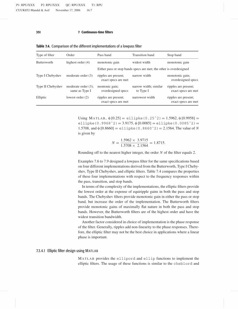
Table 7.4. Comparison of the different implementations of a lowpass filter

Type of filter Order Pass band Transition band Stop band

Butterworth highest order (4) monotonic gain widest width monotonic gain

Either pass or stop bands specs are met; the other is overdesigned

Type I Chebyshev moderate order (3) ripples are present;exact specs are met

narrow width monotonic gain;overdesigned specs

Type II Chebyshev moderate order (3);same as Type I

montonic gain;overdesigned specs

narrow width; similarto Type I

ripples are present;exact specs are met

Elliptic lowest order (2) ripples are present;exact specs are met

narrowest width ripples are present;exact specs are met

Using M A T L A B , � [0.25] = ellipke(0.25ˆ2)= 1.5962, � [0.9958] =ellipke(0.9968ˆ2)= 3.9175, � [0.0085] = ellipke(0.0085ˆ2)=1.5708, and � [0.8660] = ellipke(0.8660ˆ2)= 2.1564. The value of Nis given by

N = 1.5962 × 3.9715

1.5708 × 2.1564= 1.8715.

Rounding off to the nearest higher integer, the order N of the filter equals 2.

Examples 7.6 to 7.9 designed a lowpass filter for the same specifications basedon four different implementations derived from the Butterworth, Type I Cheby-shev, Type II Chebyshev, and elliptic filters. Table 7.4 compares the propertiesof these four implementations with respect to the frequency responses withinthe pass, transition, and stop bands.

In terms of the complexity of the implementations, the elliptic filters providethe lowest order at the expense of equiripple gains in both the pass and stopbands. The Chebyshev filters provide monotonic gain in either the pass or stopband, but increase the order of the implementation. The Butterworth filtersprovide monotonic gains of maximally flat nature in both the pass and stopbands. However, the Butterworth filters are of the highest order and have thewidest transition bandwidth.

Another factor considered in choice of implementation is the phase responseof the filter. Generally, ripples add non-linearity to the phase responses. There-fore, the elliptic filter may not be the best choice in applications where a linearphase is important.

7.3.4.1 Elliptic filter design using M ATL AB

M A T L A B provides the ellipord and ellip functions to implement theelliptic filters. The usage of these functions is similar to the cheb1ord and




0 50 100 150 200 2500

0.1778

0.40.6

0.89131Fig. 7.11. Magnitude spectrum

of the elliptic lowpass filterdesigned in Example 7.9.

cheby1 functions used to design Type I Chebyshev filters. The code to imple-ment an elliptic filter for Example 7.9 is as follows:

>> wp=50; ws=100; rp=1;rs=15;


>> [N,wn] = ellipord


% determine order and

natural freq

>> [num,den] =ellip(N,rp,rs,wn,‘s’);


coeff.

>> Ht = tf(num,den); % determine transfer

function

>> [H,w] = freqs(num,den); % determine magnitude

spectrum



Instruction II: N = 2; wn = 50;

Instruction III: num = [0.1778 0 2369.66];

den = [1.0000 48.384 2961.75];

Instruction IV: Ht = (0.1778sˆ2 + 2640)/(sˆ2 + 48.38s

+ 2962);

The magnitude spectrum is plotted in Fig. 7.11.

7.4 Frequency transformations

In Section 7.3, we designed a collection of specialized CT lowpass filters. Inthis section, we consider the design techniques for the remaining three cat-egories (highpass, bandpass, and bandstop filters) of CT filters. A commonapproach for designing CT filters is to convert the desired specifications intothe specifications of a normalized or prototype lowpass filter using a frequencytransformation that maps the required frequency-selective filter into a lowpassfilter. Based on the transformed specifications, a normalized lowpass filter isdesigned using the techniques covered in Section 7.3. The transfer functionH (S) of the normalized lowpass filter is then transformed back into the originalfrequency domain. Transformation for converting a lowpass filter to a highpass




filter is considered next, followed by the lowpass to bandpass, and lowpass tobandstop transformations.

7.4.1 Lowpass to highpass filter

The transformation that converts a lowpass filter with the transfer function H (S)into a highpass filter with transfer function H (s) is given by

S = �p

s, (7.67)

where S = � + j� represents the lowpass domain and s = � + j� representsthe highpass domain. The frequency � = �� represents the pass-band cornerfrequency for the highpass filter. In terms of the CTFT domain, Eq. (7.67) canbe expressed as follows:

� = −�p

�or � = −�p

�. (7.68)

Figure 7.12 shows the effect of applying the frequency transformation inEq. (7.68) to the specifications of a highpass filter. Equation (7.68) maps thehighpass specifications in the range −∞ < � ≤ 0 to the specifications of alowpass filter in the range 0 ≤ � < ∞. Similarly, the highpass specificationsfor the positive range of frequencies (0 < � ≤ ∞) are mapped to the lowpassspecifications within the range −∞ ≤ � < 0. Since the magnitude spectra aresymmetrical about the y-axis, the change from positive � frequencies to negative� frequencies does not affect the nature of the filter in the entire domain.

Highpass to lowpass transformationω = −ξp/ξ

1

ξs

ξp

pass band

stop band

transition band

Hhp(ξ)

−ξp −ξs

1−δp

1−δp

1+δp

1+δp

pass band stop bandtransitionband

ξ0

δs

δs

ξ

ω ω

|Hlp(ω)|

Fig. 7.12. Highpass to lowpasstransformation.




From Fig. 7.12, it is clear that Eq. (7.68), or alternatively Eq. (7.67), representsa highpass to lowpass transformation. We now exploit this transformation todesign a highpass filter.

Example 7.10Design a highpass Butterworth filter with the following specifications:

stop band (0 ≤ |� | ≤ 50 radians/s) −1 ≤ 20 log10 |H (�)| ≤ 0;

pass band (|� | > 100 radians/s) 20 log10 |H (�)| ≤ −15.

SolutionUsing Eq. (7.67) with �p = 100 radians/s to transform the specifications fromthe domain s = � + j� of the highpass filter to the domain S = � + j� of thelowpass filter, we obtain

stop band (∞ < |� | ≤ 2 radians/s) −1 ≤ 20 log10 |H (�)| ≤ 0;

pass band (|� | < 1 radian/s) 20 log10 |H (�)| ≤ 15.

The above specifications are used to design a normalized lowpass Butterworthfilter. Expressed on a linear scale, the pass-band and stop-band gains are givenby

(1 −�p) = 10−1/20 = 0.8913 and �s = 10−15/20 = 0.1778.

The gain terms Gp and Gs are given by

Gp = 1

(1 − �p)2− 1 = 1

0.89132− 1 = 0.2588

and

Gs = 1

(�s)2− 1 = 1

0.17782− 1 = 30.6327.


N = 1

2× ln(Gp/Gs)

ln(�p/�s)= 1

2× ln(0.2588/30.6327)

ln(1/2)= 3.4435.

We round off the order of the filter to the higher integer value as N = 4.Using the pass-band constraint, Eq. (7.31), the cut-off frequency of the

required Butterworth filter is given by

�c = �s

(Gs)1/2N= 2

(30.6327)1/8= 1.3039 radians/s.




0 50 100 150 200 2500

0.1778

0.40.6

0.89131Fig. 7.13. Magnitude spectrum

of the Butterworth highpassfilter designed in Example 7.10.

The poles of the lowpass filter are located at

S = �c exp

[j�

2+ j

(2n − 1)�

8

]

for 1 ≤ n ≤ 4. Substituting different values of n yields

S = [−0.4990 + j1.2047 −1.2047 + j0.4990 −1.2047

−j0.4990 −0.4990 − j1.2047].

The transfer function of the lowpass filter is given by

H (S) = K

(S+0.4490−j1.2047)(S+0.4490+j1.2047)(S+1.2047−j0.4990)(S+1.2047+j0.4990)

or

H (S) = K

S4 + 3.4074S3 + 5.8050S2 + 5.7934S + 2.8909.

To ensure a dc gain of unity for the lowpass filter, we set K = 2.8909. Thetransfer function of a unity gain lowpass filter is given by

H (S) = 2.8909

S4 + 3.4074S3 + 5.8050S2 + 5.7934S + 2.8909.

To derive the transfer function of the required highpass filter, we use Eq. (7.67)with �p = 100 radians/s. The transfer function of the highpass filter is given by

H (s) = H (S)|S=100/s

= 2.8909

(100/s)4 + 3.4074(100/s)3 + 5.8050(100/s)2 + 5.7934(100/s) + 2.8909

or

H (s)= s4

s4 + 2.004 × 102s3 + 2.008 × 104s2 + 1.179 × 106s + 3.459 × 107.

The magnitude spectrum of the highpass filter is given in Fig. 7.13, whichconfirms that the given specifications are satisfied.

7.4.1.1 M ATL AB code for designing highpass filters

The M A T L A B code for the design of the highpass filter required inExample 7.10 using the Butterworth, Type I Chebyshev, Type II Chebyshev,




and elliptic implementations is included below. In each case, M A T L A B auto-matically designs the highpass filter. No explicit transformations are needed.

>> % Matlab code for designing highpass filter

>> wp=100; ws=50; Rp=1; Rs=15; % design specifications

>> % Butterworth filter

>> [N, wc] =buttord(wp,ws,Rp,Rs,‘s’);

% determine order and

cut off

>> [num1,den1] =butter(N,wc,‘high’,‘s’);

% determine transfer

function

>> H1 = tf(num1,den1);

>> %%%%% % Type I Chebyshev

filter

>> [N, wn] =cheb1ord(wp,ws,Rp,Rs,‘s’);

>> [num2,den2] =cheby1(N,Rp,wn,‘high’,‘s’);


>> %%%%% % Type II Chebyshev

filter

>> [N,wn] =cheb2ord(wp,ws,Rp,Rs,‘s’) ;

>> [num3,den3] =cheby2(N,Rs,wn,‘high’,‘s’) ;


>> %%%%% % Elliptic filter

>> [N,wn] =ellipord(wp,ws,Rp,Rs,‘s’) ;

>> [num4,den4] =ellip(N,Rp,Rs,wn,‘high’,‘s’) ;


In the above code, note thatwp > ws. Also, an additional argument of‘high’is included in the design statements for different filters, which is used to specifya highpass filter. The aforementioned M A T L A B code results in the followingtransfer functions for the different implementations:

Butterworth

H (s) = s4

s4 + 2.004 × 102s3 + 2.008 × 104s2 + 1.179 × 106s + 3.459 × 107;

Type I Chebyshev H (s) = s3

s3 + 252.1s2 + 2.012 × 104s + 2.035 × 106;

Type II Chebyshev H (s) = s3 + 3.027 × 103s

s3 + 113.5s2 + 9.473 × 103s + 3.548 × 105;

elliptic H (s) = 0.8903s2 + 1501

s2 + 81.68s + 8441.




The transfer function for the Butterworth filter is the same as that derived byhand in Example 7.9.

7.4.2 Lowpass to bandpass filter

The transformation that converts a lowpass filter with the transfer function H (S)into a bandpass filter with transfer function H (s) is given by

S = s2 + �p1�p2

s(�p2 − �p1), (7.69)

where S = S = � + j� represents the lowpass domain and s = � + j� repre-sents the bandpass domain. The frequency � = �p1 and �p2 represents the twopass-band corner frequencies for the bandpass filter with �p2 > �p1. In terms ofthe CTFT variables � and � , Eq. (7.69) can be expressed as follows:

�s1 = �p1�p2 − �2

�(�p2 − �p1). (7.70)

From Eq. (7.70), it can be shown that the pass-band corner frequencies �p1 and−�p2 of the bandpass filter are both mapped in the lowpass domain to � = 1,whereas the pass-band corner frequencies −�p1 and �p2 are mapped to � = −1.Also, the pass band �p1 ≤ |� | = �p2 of the bandpass filter is mapped to thepass band −1 ≤ |� | ≤ 1 of the lowpass filter. These results can be confirmedby substituting different values for the bandpass domain frequencies � andevaluating the corresponding lowpass domain frequencies.

Considering the stop-band corner frequencies of the bandpass filter,Eq. (7.70) can be used to show that the stop-band corner frequency ±�s1 ismapped to

� =∣∣∣∣ �p1�p2 − �2

s1

�s1(�p2 − �p1)

∣∣∣∣ , (7.71)

and that the stop-band corner frequency ±�s2 is mapped to

�s2 =∣∣∣∣ �p1�p2 − �2

s2

�s2(�p2 − �p1)

∣∣∣∣ . (7.72)

As a lower value for the stop-band frequency for the lowpass filter leads tomore stringent requirements, the stop-band corner frequency for the lowpassfilter is selected from the minimum of the two values computed in Eqs (7.71)and (7.72). Mathematically, this implies that

�s = min(�s1, �s2). (7.73)

Example 7.11 designs a bandpass filter.




Example 7.11Design a bandpass Butterworth filter with the following specifications:

stop band I (0 ≤ |� | ≤ 50 radians/s) 20 log10 |H (�)| ≤ −20;

pass band (100 ≤ |� | ≤ 200 radians/s) −2 ≤ 20 log10 |H (�)| ≤ 0;

stop band II (|� | ≥ 380 radians/s) 20 log10 |H (�)| ≤ −20.

SolutionFor �p1 = 100 radians/s and �p2 = 200 radians/s, Eq. (7.70) becomes

� = 2 × 104 − �2

100�,

to transform the specifications from the domain s = � + j� of the bandpassfilter to the domain S = � + j� of the lowpass filter. The specifications for thenormalized lowpass filter are given by

pass band (0 ≤ |� | < 1 radian/s) −2 ≤ 20 log10 |H (�)| ≤ 0;

stop band (|� | ≥ min(3.2737, 3.5) radians/s 20 log10 |H (�)| ≤ −20.

The above specifications are used to design a normalized lowpass Butterworthfilter. Expressed on a linear scale, the pass-band and stop-band gains are givenby

(1 − �p) = 10−2/20 = 0.7943 and �s = 10−20/20 = 0.1.

The gain terms Gp and Gs are given by

Gp = 1

(1 − �p)2− 1 = 1

0.79432− 1 = 0.5850

and

Gs = 1

(�s)2− 1 = 1

0.17782− 1 = 99.


N = 1

2× ln(Gp/Gs)

ln(�p/�s)= 1

2× ln(0.5850/99)

ln(1/3.2737)= 2.1232.

We round off the order of the filter to the higher integer value as N = 3.Using the stop-band constraint, Eq. (7.31), the cut-off frequency of the low-

pass Butterworth filter is given by

�c = �s

(Gs)1/2N= 3.2737

(99)1/6= 1.5221 radians/s.


S = �c exp

[j�

2+ j

(2n − 1)�

6

]




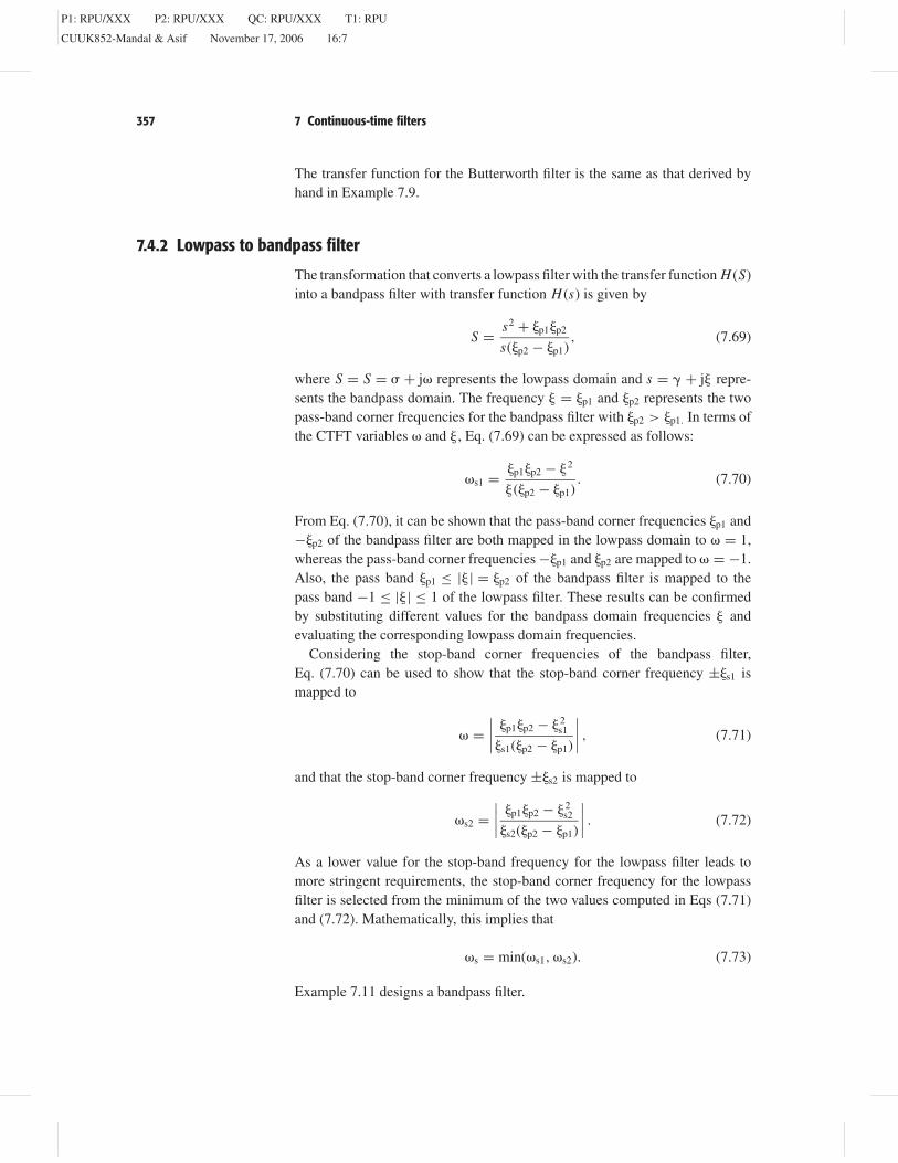
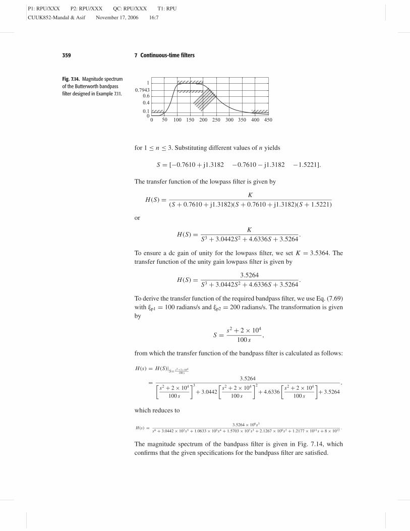
0 50 100 150 200 250 300 350 400 4500

0.1

0.40.6

0.79431

Fig. 7.14. Magnitude spectrumof the Butterworth bandpassfilter designed in Example 7.11.

for 1 ≤ n ≤ 3. Substituting different values of n yields

S = [−0.7610 + j1.3182 −0.7610 − j1.3182 −1.5221].


H (S) = K

(S + 0.7610 + j1.3182)(S + 0.7610 + j1.3182)(S + 1.5221)

or

H (S) = K

S3 + 3.0442S2 + 4.6336S + 3.5264.

To ensure a dc gain of unity for the lowpass filter, we set K = 3.5364. Thetransfer function of the unity gain lowpass filter is given by

H (S) = 3.5264

S3 + 3.0442S2 + 4.6336S + 3.5264.

To derive the transfer function of the required bandpass filter, we use Eq. (7.69)with �p1 = 100 radians/s and �p2 = 200 radians/s. The transformation is givenby

S = s2 + 2 × 104

100 s,

from which the transfer function of the bandpass filter is calculated as follows:

H (s) = H (S)|S= s2+2×104

100 s

= 3.5264[s2 + 2 × 104

100 s

]3

+ 3.0442

[s2 + 2 × 104

100 s

]2

+ 4.6336

[s2 + 2 × 104

100 s

]+ 3.5264

,

which reduces to

H (s) = 3.5264 × 106s3

s6 + 3.0442 × 102s5 + 1.0633 × 105s4 + 1.5703 × 107s3 + 2.1267 × 109s2 + 1.2177 × 1011s + 8 × 1012.

The magnitude spectrum of the bandpass filter is given in Fig. 7.14, whichconfirms that the given specifications for the bandpass filter are satisfied.




7.4.2.1 M ATL AB code for designing bandpass filters

The M A T L A B code for the design of the bandpass filter required inExample 7.11 using the Butterworth, Type I Chebyshev, Type II Chebyshev,and elliptic implementations is as follows:

>> % MATLAB code for designing bandpass filter

>> wp=[100 200]; ws=[50 380]; Rp=2;Rs=20;

% Specifications

>> % Butterworth filter

>> [N, wc] = buttord(wp,ws,Rp,Rs,‘s’);

>> [num1,den1] = butter(N,wc,‘s’);


>> % Type I Chebyshev filter

>> [N, wn] = cheb1ord(wp,ws,Rp,Rs,‘s’);

>> [num2,den2] = cheby1(N,Rp,wn,‘s’);


>> % Type II Chebyshev filter

>> [N,wn] = cheb2ord(wp,ws,Rp,Rs,‘s’);

>> [num3,den3] = cheby2(N,Rs,wn,‘s’);


>> % Elliptic filter

>> [N,wn] = ellipord(wp,ws,Rp,Rs,‘s’);

>> [num4,den4] = ellip(N,Rp,Rs,wn,‘s’);


The type of filter is specified by the dimensions of the pass-band and stop-bandfrequency vectors. Since wp and ws are both vectors, M A T L A B knows thateither a bandpass or bandstop filter is being designed. From the range of thevalues within wp and ws, M A T L A B is also able to differentiate whether abandpass or a bandstop filter is being specified. In the above example, sincethe range (50–380 Hz) of frequencies specified within the stop-band frequencyvector ws exceeds the range (100–200 Hz) specified within the pass-band fre-quency vector wp, M A T L A B is able to make the final determination that abandpass filter is being designed. For a bandstop filter, the converse would holdtrue.

The aforementioned M A T L A B code produces bandpass filters with the fol-lowing transfer functions:

Butterworth H (s) = 3.526×106s4

s6+304.4s5+1.063×105s4+1.57×107s3+2.127×109s2+1.218×1011s+8×1012;

Type I Chebyshev H (s) = 6.538 × 103s2

s4 + 80.38s3 + 4.8231 × 104s2 + 1.608 × 106s + 4 × 108;

Type II Chebyshev H (s) = 0.1s4 + 1.801 × 104s2 + 4 × 107

s4 + 1.588 × 102s3 + 5.4010 × 104s2 + 3.176 × 106s + 4 × 108;

elliptic H (s) = 0.1s4 + 1.101 × 104s2 + 4 × 107

s4 + 74.67s3 + 4.8819 × 104s2 + 1.493 × 106s + 4 × 108.




Note that the transfer function for the bandpass Butterworth filter is the sameas that derived by hand in Example 7.9.

7.4.3 Lowpass to bandstop filter

The transformation to convert a lowpass filter with the transfer function H (S)into a bandstop filter with transfer function H (s) is given by the followingexpression:

S = s(�p2 − �p1)

s2 + �p1�p2, (7.74)

where S = S = � + j� represents the lowpass domain and s = � + j� rep-resents the bandstop domain. The frequency � = �p1 and �p2 represents thetwo pass-band corner frequencies for the bandpass filter with �p2 > �p1. Notethat the transformation in Eq. (7.74) is the inverse of the lowpass to bandpasstransformation specified in Eq. (7.69).

In terms of the CTFT domain, Eq. (7.74) can be expressed as follows:

� = �(�p2 − �p1)

�p1�p2 − �2, (7.75)

which can be used to confirm that Eq. (7.74) is indeed a lowpass to bandstoptransformation.

As for the bandpass filter, Eq. (7.75) leads to two different values of thestop-band frequencies,

�s1 =∣∣∣∣�s1(�p2 − �p1)

�p1�p2 − �2s1

∣∣∣∣ and �s2 =∣∣∣∣�s2(�p2 − �p1)

�p1�p2 − �2s2

∣∣∣∣ (7.76)

for the lowpass filter. The smaller of the two values is selected as the stop-bandcorner frequency for the normalized lowpass filter. Example 7.12 designs abandstop filter.

Example 7.12Design a bandstop Butterworth filter with the following specifications:

pass band I (0 ≤ |� | ≤ 100 radians/s) −2 ≤ 20 log10 |H (�)| ≤ 0;

stop band (150 ≤ |� | ≤ 250 radians/s) 20 log10 |H (�)| ≤ −20;

pass band II (|� | ≥ 370 radians/s) −2 ≤ 20 log10 |H (�)| ≤ 0.

SolutionFor �p1 = 100 radians/s and �p2 = 370 radians/s, Eq. (7.70) becomes

� = 270�

3.7 × 104 − �2,

to transform the specifications from the domain s = � + j� of the bandstopfilter to the domain S = � + j� of the lowpass filter. The specifications for the




normalized lowpass filter are given by

pass band (0 ≤ |� | < 1 radian/s) − 2 ≤ 20 log10 |H (�)| ≤ 0;

stop band (|� | ≥ min(2.7931, 2.6471) radians/s 20 log10 |H (�)| ≤ −20.

The above specifications are used to design a normalized lowpass Butterworthfilter. Since the pass-band and stop-band gains of the transformed lowpass filterare the same as the ones used in Example 7.11, i.e.

(1 − �p) = 10−2/20 = 0.7943 and �s = 10−20/20 = 0.1,

with gain terms

Gp = 0.5850 and Gs = 99,

the order N = 3 of the Butterworth filter is the same as in Example 7.11.Using the stop-band constraint, Eq. (7.31), the cut-off frequency of the low-

pass Butterworth filter is given by

�c = �s

(Gs)1/2N= 2.6471

(99)1/6= 1.2307 radians/s.


S = �c exp

[j�

2+ j

(2n − 1)�

6

]for 1 ≤ n ≤ 3. Substituting different values of n yields

S = [−0.6153 + j0.06581 −0.6153 − j0.06581 −1.2307].


H (S) = K

(S + 0.6153 − j0.06581)(S + 0.6153 + j0.06581)(S + 1.2307)or

H (S) = K

S3 + 2.4614S2 + 3.0292S + 1.8640.

To ensure a dc gain of unity for the lowpass filter, we set K = 1.8640. Thetransfer function of the unity gain lowpass filter is given by

H (S) = 1.8640

S3 + 2.4614S2 + 3.0292S + 1.8640.

To derive the transfer function of the required bandstop filter, we use Eq. (7.74)with �p1 = 100 radians/s and �p2 = 370 radians/s. The transformation is givenby

S = 270s

s2 + 3.7 × 104,

with the transfer function of the bandstop filter is given by

H (s) = H (S)|S= 270ss2+3.7×104

= 1.8640[270s

s2+3.7×104

]3

+ 2.4641

[270s

s2+3.7×104

]2

+ 3.0292

[270s

s2+3.7×104

]+1.8640

,




0 50 100 150 200 250 300 350 400 450 5000

0.1

0.40.6

0.79431

Fig. 7.15. Magnitude spectrumof the Butterworth bandstopfilter designed in Example 7.12.

which reduces to

H (s) = s6+1.11×105s4+4.107×109s2+5.065×1013

s6+4.388×102s5+2.0737×105s4+4.302×107s3+7.673×109s2+6 × 1011s+5.065×1013.

The magnitude spectrum of the bandstop filter is included in Fig. 7.15, whichconfirms that the given specifications are satisfied.

7.4.3.1 M ATL AB code for designing bandstop filters

The M A T L A B code for the design of the bandstop filter required inExample 7.12 using the Butterworth, Type I Chebyshev, Type II Chebyshev,and elliptic implementations is as follows:

% MATLAB code for designing bandstop filter

>> wp=[100 370]; ws=[150 250]; Rp=2;

Rs=20;

% Specifications

>> % Butterworth Filter

>> [N, wn] = buttord(wp,ws,Rp,Rs,‘s’);

>> [num1,den1] = butter(N,wn, ‘stop’,‘s’);


>> % Type I Chebyshev filter

>> [N, wn] = cheb1ord(wp,ws,Rp,Rs,‘s’);

>> [num2,den2] = cheby1(N,Rp,wn,

‘stop’,‘s’);


>> % Type II Chebyshev filter

>> [N,wn] = cheb2ord(wp,ws,Rp,Rs,‘s’);

>> [num3,den3] = cheby2(N,Rs,wn,



>> % Elliptic filter

>> [N,wn] = ellipord(wp,ws,Rp,Rs,‘s’);

>> [num4,den4] = ellip(N,Rp,Rs,wn,



The aforementioned M A T L A B code produces the following transfer functions




for the four filters:

Butterworth H (s) = s6 +1.125×105s4 +4.219×109s2 +5.273×1013

s6 +430.2s5 +2.05×105s4 +4.221×107s3 +7.688×109s2 +6.049×1011s+5.273×1013;

Type I Chebyshev H (s) = 0.7943s4 + 5.957 × 104s2 + 1.117 × 109

s4 + 262.4s3 + 1.627 × 105s2 + 9.839 × 106s + 1.406 × 109;

Type II Chebyshev H (s) = 0.7943s4 + 8.015 × 104s2 + 1.406 × 109

s4 + 304.5s3 + 1.265 × 105s2 + 1.142 × 106s + 1.406 × 109;

elliptic H (s) = 0.7943s4 + 6.776 × 104s2 + 1.117 × 109

s4 + 227.5s3 + 1.568 × 105s2 + 8.53 × 106s + 1.406 × 109.

7.5 Summary

Chapter 7 defines the CT filters as LTI systems used to transform the frequencycharacteristics of the CT signals in a predefined manner. Based on the magnitudespectrum |H (�)|, Section 7.1 classifies the frequency-selective filters into fourdifferent categories.

(1) An ideal lowpass filter removes frequency components above the cut-offfrequency �c from the input signal, while retaining the lower frequencycomponents � ≤ �c.

(2) An ideal highpass filter is the converse of the lowpass filter since it removesfrequency components below the cut-off frequency �c from the input signal,while retaining the higher frequency components � ≤ �c.

(3) An ideal bandpass filter retains a selected range of frequency componentsbetween the lower cut-off frequency �c1 and the upper cutoff frequency�c2 of the filter. All other frequency components are eliminated from theinput signal.

(4) A bandstop filter is the converse of the bandpass filter, which rejects allfrequency components between the lower cut-off frequency �c1 and theupper cut-off frequency �c2 of the filter. All other frequency componentsare retained at the output of the bandstop filter.

The ideal frequency filters are not physically realizable. Section 7.2 introducespractical implementations of the ideal filters obtained by introducing ripplesin the pass and stop bands. A transition band is also included to eliminate thesharp transition between the pass and stop bands.

In Section 7.3, we considered the design of practical lowpass filters. We pre-sented four implementations of practical filters: Butterworth, Type I Chebyshev,Type II Chebyshev, and elliptic filters, for which the design algorithms werecovered. The Butterworth filters provide a maximally flat gain within the passband but have a higher-order N than the Chebyshev and elliptic filters designedwith the same specifications. By introducing ripples within the pass band,Type I Chebyshev filters reduce the required order N of the designed filter.Alternatively, Type II Chebyshev filters introduce ripples within the stop bandto reduce the order N of the filter. The elliptic filters allow ripples in both the




pass and stop bands to derive a filter with the lowest order N among the fourimplementations. M A T L A B instructions to design the four implementationsare also presented in Section 7.3.

In Section 7.4, we covered three transformations for converting a highpassfilter to a lowpass filter, a lowpass to a bandpass filter, and a bandstop to a lowpassfilter. Using these transformations, we were able to map the specifications ofany type of the frequency-selective filters in terms of a normalized lowpassfilter. After designing the normalized lowpass filter using the design algorithmscovered in Section 7.3, the transfer function of the lowpass filter is transformedback into the original domain of the frequency-selective filter.

Problems

7.1 Determine the impulse response of an ideal bandpass filter and an idealbandstop filter. In each case, assume a gain of A within the pass bands andcut off frequencies of �c1 and �c2.

7.2 Derive and sketch the location of the poles for the Butterworth filters oforders N = 12 and 13 in the complex s-plane.

7.3 Show that a lowpass Butterworth filter with an odd value of order N willalways have at least one pole on the real axis in the complex s-plane.

7.4 Show that all complex poles of the lowpass Butterworth filter occur inconjugate pairs.

7.5 Show that the locations of poles for the Type I Chebyshev polynomialTN (�) of order N is given by

�n = cos

[(2n + 1)�

2N

]

for |�| ≤ 1 and |�| > 1.

7.6 Show that the roots of the characteristic equation

1 + ε2T 2N ( j/s) = 0

for the Type II Chebyshev filter are the inverse of the roots of the charac-teristic equation

1 + ε2T 2N (s/j) = 0

for the Type I Chebyshev filter.

7.7 Design a Butterworth lowpass filter for the following specifications:

pass band (0 ≤ |�| ≤ 10 radians/s) 0.9 ≤ |H (�)| ≤ 1;

stop band (|�| > 20 radians/s) |H (�)| ≤ 0.10,




by enforcing the pass-band requirements. Repeat for the stop-bandrequirements. Sketch the magnitude spectrum and confirm that the mag-nitude spectrum satisfies the design specifications.

7.8 Repeat Problem 7.7 for the following specifications:

pass band (0 ≤ |�| ≤ 50 radians/s) −1 ≤ 20 log10 |H (�)| ≤ 0;

stop band (|�| > 65 radians/s) 20 log10 |H (�)| ≤ −25.

7.9 Repeat (a) Problem 7.7 and (b) Problem 7.8 for the Type I Chebyshevfilter.

7.10 Repeat (a) Problem 7.7 and (b) Problem 7.8 for the Type II Chebyshevfilter.

7.11 Determine the order of the elliptic filters for the specifications includedin (a) Problem 7.7 and (b) Problem 7.8.

7.12 Using the results in Problems 7.7–7.11, compare the implementationcomplexity of the Butterworth, Type I Chebyshev, Type II Chebyshev,and elliptic filters for the specifications included in (a) Problem 7.7 and(b) Problem 7.8.

7.13 By selecting the corner frequencies of the pass and stop bands, show thatthe transformation

S = s(�p2 − �p1)

s2 + �p1�p2

maps a bandstop filter into a normalized lowpass filter.

7.14 Design a Butterworth highpass filter for the following specifications:

stop band (0 ≤ |�| ≤ 15 radians/s) |H (�)| ≤ 0.15;

pass band (|�| > 30 radians/s) 0.85 ≤ |H (�)| ≤ 1.

Sketch the magnitude spectrum and confirm that it satisfies the designspecifications.

7.15 Repeat Problem 7.14 for the Type I Chebyshev filter.

7.16 Repeat Problem 7.14 for the Type II Chebyshev filter.

7.17 Design a Butterworth bandpass filter for the following specifications:

stop band I (0 ≤ |� | ≤ 100 radians/s) 20 log10 |H (�)| ≤ −15;

Pass band (100 ≤ |� | ≤ 150 radians/s) −1 ≤ 20 log10 |H (�)| ≤ 0;

stop band II (|� | ≥ 175 radians/s) 20 log10 |H (�)| ≤ −15.







7.20 Design a Butterworth bandstop filter for the following specifications:

pass band I (0 ≤ |� | ≤ 25 radians/s) −4 ≤ 20 log10 |H (�)| ≤ 0;

stop band (100 ≤ |� | ≤ 250 radians/s) 20 log10 |H (�)| ≤ −20;

pass band II (|� | ≥ 325 radians/s) −4 ≤ 20 log10 |H (�)| ≤ 0.




7.23 Determine the transfer function of the four implementations: (a) Butter-worth, (b) Type I Chebyshev, (c) Type II Chebyshev, and (d) elliptic, ofthe lowpass filter specified in Problem 7.7 using M A T L A B . Plot the fre-quency characteristics and confirm that the specifications are satisfied bythe designed implementations.

7.24 Determine the transfer function of the four implementations: (a) Butter-worth, (b) Type I Chebyshev, (c) Type II Chebyshev, and (d) elliptic, ofthe lowpass filter specified in Problem 7.8 using M A T L A B . Plot the fre-quency characteristics and confirm that the specifications are satisfied bythe designed implementations.

7.25 Determine the transfer function of the four implementations: (a) Butter-worth, (b) Type I Chebyshev, (c) Type II Chebyshev, and (d) elliptic, ofthe highpass filter specified in Problem 7.14 using M A T L A B . Plot thefrequency characteristics and confirm that the specifications are satisfiedby the designed implementations.

7.26 Determine the transfer function of the four implementations (a) Butter-worth, (b) Type I Chebyshev, (c) Type II Chebyshev, and (d) elliptic, ofthe bandpass filter specified in Problem 7.17 using M A T L A B . Plot thefrequency characteristics and confirm that the specifications are satisfiedby the designed implementations.

7.27 Determine the transfer function of the four implementations: (a) Butter-worth, (b) Type I Chebyshev, (c) Type II Chebyshev, and (d) elliptic, ofthe bandstop filter specified in Problem 7.20 using M A T L A B . Plot thefrequency characteristics and confirm that the specifications are satisfiedby the designed implementations.

Documents

Continuous-time ﬁlters - Veřejné služby … RPU/XXX P2: RPU/XXX QC: RPU/XXX T1: RPU CUUK852-Mandal & Asif November 17, 2006 16:7 324 Part II Continuous-time signals and systems