Continuous Probability, RVs, Distributions

EECS 126 Fall 2019

September 17, 2019

Agenda

Announcements

ReviewContinuous Probability DefinitionsCumulative Distribution Functions

DistributionsUniformExponentialGaussian

Analogs to Discrete Probability / RVs

Derived Distributions

Announcements

I HW3 AND Lab2 are due Friday (9/20).

I Feel free to come to Lab Party with HW questions onThursday!

I HW4 will be optional to give you more time to study. We stillrecommend reading and attempting the problems.

I Midterm 1 is coming up quick on 9/26! You can find pastexams on the Exams page of the website.

Probability Densities

In a continuous space, we describe distributions with probabilitydensity functions (PDFs) rather than assigned probability values.

A valid probability density of a continuous random variable X in R,fX (x), requires

I Non-negativity: ∀x ∈ R fX (x) ≥ 0

I Normalized:∫R fX (x)dx = 1

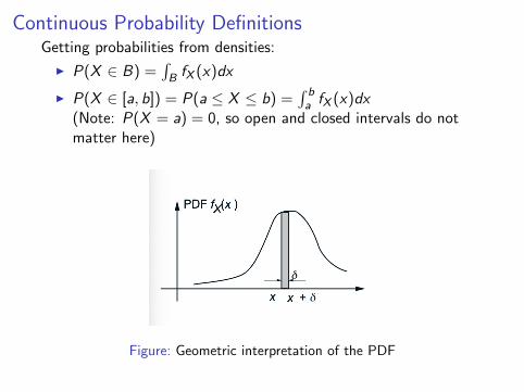
Continuous Probability DefinitionsGetting probabilities from densities:

I P(X ∈ B) =∫B fX (x)dx

I P(X ∈ [a, b]) = P(a ≤ X ≤ b) =∫ ba fX (x)dx

(Note: P(X = a) = 0, so open and closed intervals do notmatter here)

Figure: Geometric interpretation of the PDF

Questions

Suppose we uniformly sample a point in a ball of radius 1. What isthe

I Probability of picking the origin?

I Probability density of picking the origin?

I Probability of picking a point on the surface?

I Probability of picking a point within a radius of 12?

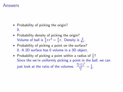
Answers

I Probability of picking the origin?0.

I Probability density of picking the origin?Volume of ball is 4

3πr3 = 4

3π. Density is 34π .

I Probability of picking a point on the surface?0. A 2D surface has 0 volume in a 3D object.

I Probability of picking a point within a radius of 12?

Since the we’re uniformly picking a point in the ball, we can

just look at the ratio of the volumes.4π3( 12)3

4π3

= 18 .

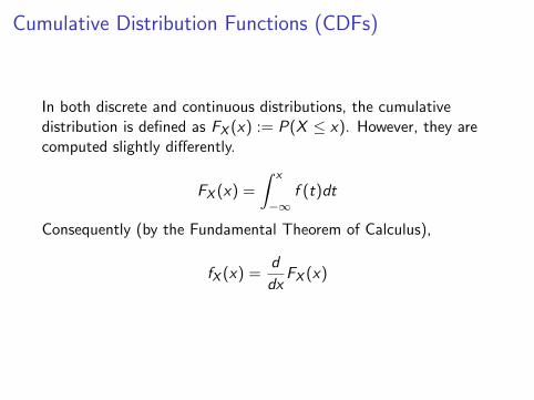
Cumulative Distribution Functions (CDFs)

In both discrete and continuous distributions, the cumulativedistribution is defined as FX (x) := P(X ≤ x). However, they arecomputed slightly differently.

FX (x) =

∫ x

−∞f (t)dt

Consequently (by the Fundamental Theorem of Calculus),

fX (x) =d

dxFX (x)

More familiar definitions

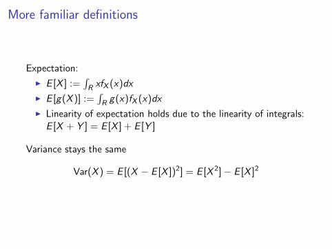
Expectation:

I E [X ] :=∫R xfX (x)dx

I E [g(X )] :=∫R g(x)fX (x)dx

I Linearity of expectation holds due to the linearity of integrals:E [X + Y ] = E [X ] + E [Y ]

Variance stays the same

Var(X ) = E [(X − E [X ])2] = E [X 2]− E [X ]2

Questions

Let R be equal to the distance from the origin of a point randomlysampled on a unit ball. What is the

I CDF of R?

I PDF of R?

I Expectation of R?

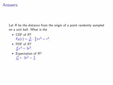
Answers

Let R be the distance from the origin of a point randomly sampledon a unit ball. What is the

I CDF of R?FR(r) = 3

4π ·43πr

3 = r3.

I PDF of R?ddr r

3 = 3r2.

I Expectation of R?∫ 10 r · 3r2 = 3

4 .

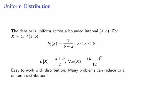
Uniform Distribution

The density is uniform across a bounded interval (a, b). ForX ∼ Unif (a, b)

fX (x) =1

b − a, a < x < b

E [X ] =a + b

2, Var(X ) =

(b − a)2

12

Easy to work with distribution. Many problems can reduce to auniform distribution!

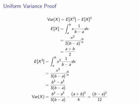
Uniform Variance Proof

Var(X ) = E [X 2]− E [X ]2

E [X ] =

∫ b

ax

1

b − adx

=x2

2(b − a)|ba

=a + b

2

E [X 2] =

∫ b

ax2

1

b − adx

=x3

3(b − a)|ba

=b3 − a3

3(b − a)

Var(X ) =b3 − a3

3(b − a)− (a + b)2

4=

(b − a)2

12

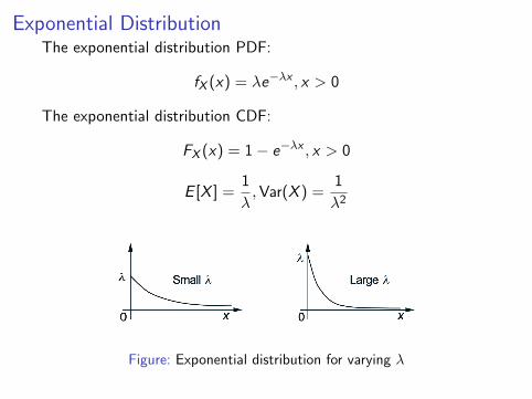
Exponential DistributionThe exponential distribution PDF:

fX (x) = λe−λx , x > 0

The exponential distribution CDF:

FX (x) = 1− e−λx , x > 0

E [X ] =1

λ,Var(X ) =

1

λ2

Figure: Exponential distribution for varying λ

Memoryless Property

The defining characteristic of the exponential is the memorylessproperty. Recall the memoryless property is:

P(X > x + a|X > x) = P(X > a)

Think about banging your head on the wall.

What distribution does this remind you of?

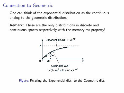
Connection to Geometric

One can think of the exponential distribution as the continuousanalog to the geometric distribution.

Remark: These are the only distributions in discrete andcontinuous spaces respectively with the memoryless property!

Figure: Relating the Exponential dist. to the Geometric dist.

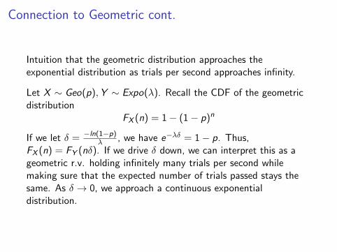
Connection to Geometric cont.

Intuition that the geometric distribution approaches theexponential distribution as trials per second approaches infinity.

Let X ∼ Geo(p),Y ∼ Expo(λ). Recall the CDF of the geometricdistribution

FX (n) = 1− (1− p)n

If we let δ = −ln(1−p)λ , we have e−λδ = 1− p. Thus,

FX (n) = FY (nδ). If we drive δ down, we can interpret this as ageometric r.v. holding infinitely many trials per second whilemaking sure that the expected number of trials passed stays thesame. As δ → 0, we approach a continuous exponentialdistribution.

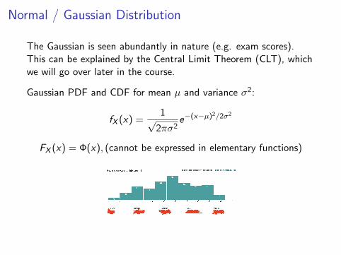
Normal / Gaussian Distribution

The Gaussian is seen abundantly in nature (e.g. exam scores).This can be explained by the Central Limit Theorem (CLT), whichwe will go over later in the course.

Gaussian PDF and CDF for mean µ and variance σ2:

fX (x) =1√

2πσ2e−(x−µ)

2/2σ2

FX (x) = Φ(x), (cannot be expressed in elementary functions)

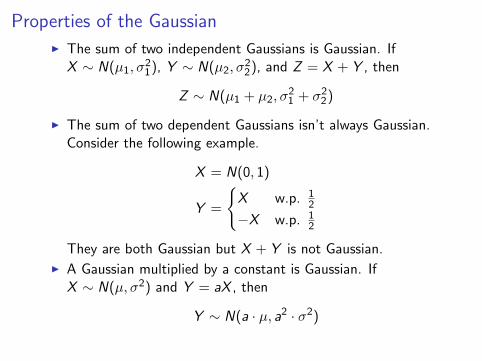
Properties of the Gaussian

I The sum of two independent Gaussians is Gaussian. IfX ∼ N(µ1, σ

21), Y ∼ N(µ2, σ

22), and Z = X + Y , then

Z ∼ N(µ1 + µ2, σ21 + σ22)

I The sum of two dependent Gaussians isn’t always Gaussian.Consider the following example.

X = N(0, 1)

Y =

{X w.p. 1

2

−X w.p. 12

They are both Gaussian but X + Y is not Gaussian.

I A Gaussian multiplied by a constant is Gaussian. IfX ∼ N(µ, σ2) and Y = aX , then

Y ∼ N(a · µ, a2 · σ2)

Scaling to the Standard Gaussian

I The properties on the previous slide allow us to convert anyGaussian into the standard Gaussian.

I If X ∼ N(µ, σ2), then

Z =X − µσ

is distributed with Z ∼ N(0, 1).

I Intuition: I got 1 SD on midterm 1.

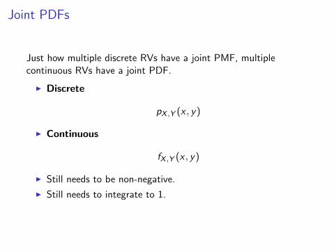
Joint PDFs

Just how multiple discrete RVs have a joint PMF, multiplecontinuous RVs have a joint PDF.

I Discrete

pX ,Y (x , y)

I Continuous

fX ,Y (x , y)

I Still needs to be non-negative.

I Still needs to integrate to 1.

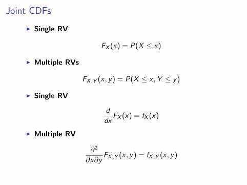
Joint CDFs

I Single RV

FX (x) = P(X ≤ x)

I Multiple RVs

FX ,Y (x , y) = P(X ≤ x ,Y ≤ y)

I Single RV

d

dxFX (x) = fX (x)

I Multiple RV

∂2

∂x∂yFX ,Y (x , y) = fX ,Y (x , y)

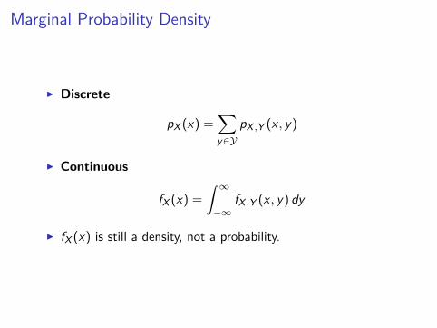
Marginal Probability Density

I Discrete

pX (x) =∑y∈Y

pX ,Y (x , y)

I Continuous

fX (x) =

∫ ∞−∞

fX ,Y (x , y) dy

I fX (x) is still a density, not a probability.

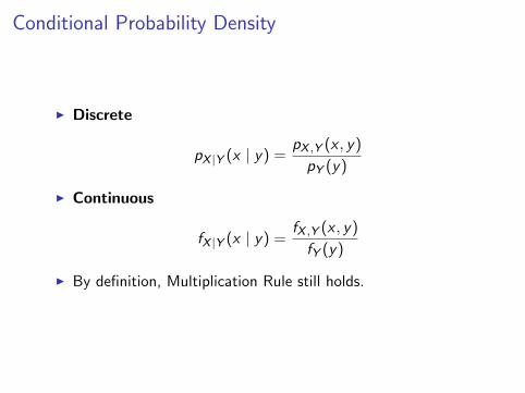
Conditional Probability Density

I Discrete

pX |Y (x | y) =pX ,Y (x , y)

pY (y)

I Continuous

fX |Y (x | y) =fX ,Y (x , y)

fY (y)

I By definition, Multiplication Rule still holds.

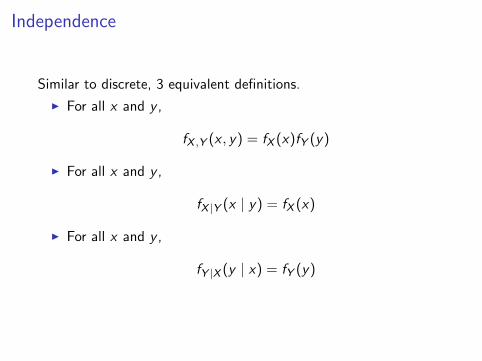
Independence

Similar to discrete, 3 equivalent definitions.

I For all x and y ,

fX ,Y (x , y) = fX (x)fY (y)

I For all x and y ,

fX |Y (x | y) = fX (x)

I For all x and y ,

fY |X (y | x) = fY (y)

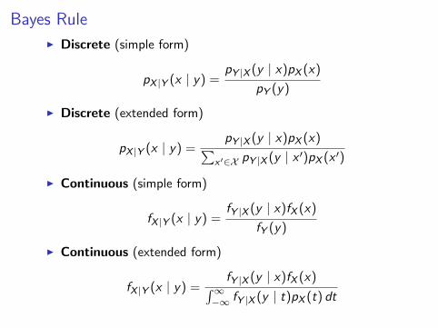
Bayes Rule

I Discrete (simple form)

pX |Y (x | y) =pY |X (y | x)pX (x)

pY (y)

I Discrete (extended form)

pX |Y (x | y) =pY |X (y | x)pX (x)∑

x ′∈X pY |X (y | x ′)pX (x ′)

I Continuous (simple form)

fX |Y (x | y) =fY |X (y | x)fX (x)

fY (y)

I Continuous (extended form)

fX |Y (x | y) =fY |X (y | x)fX (x)∫∞

−∞ fY |X (y | t)pX (t) dt

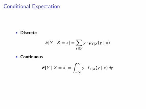
Conditional Expectation

I Discrete

E [Y | X = x ] =∑y∈Y

y · pY |X (y | x)

I Continuous

E [Y | X = x ] =

∫ ∞−∞

y · fY |X (y | x) dy

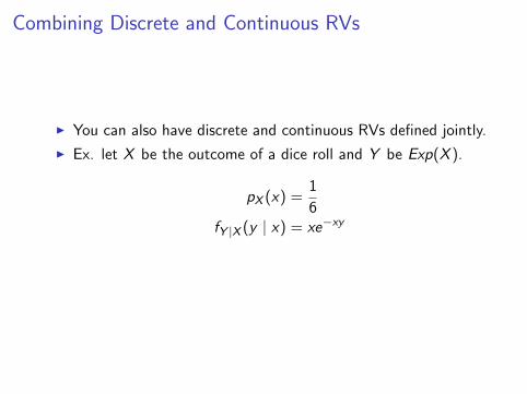
Combining Discrete and Continuous RVs

I You can also have discrete and continuous RVs defined jointly.

I Ex. let X be the outcome of a dice roll and Y be Exp(X ).

pX (x) =1

6fY |X (y | x) = xe−xy

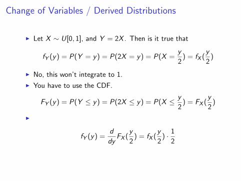
Change of Variables / Derived Distributions

I Let X ∼ U[0, 1], and Y = 2X . Then is it true that

fY (y) = P(Y = y) = P(2X = y) = P(X =y

2) = fX (

y

2)

I No, this won’t integrate to 1.

I You have to use the CDF.

FY (y) = P(Y ≤ y) = P(2X ≤ y) = P(X ≤ y

2) = FX (

y

2)

I

fY (y) =d

dyFX (

y

2) = fX (

y

2) · 1

2

References

Introduction to probability. DP Bertsekas, JN Tsitsiklis - 2002