Embed Size (px)
Citation preview

Continuous Blending of Dry Pharmaceutical
Powders
by
Lakshman PernenkilB. Tech & M.Tech, Chemical Engineering, IIT Madras, India, 2003
Submitted to the Department of Chemical Engineeringin partial fulfillment of the requirements for the degree of
Doctor of Philosophy in Chemical Engineering Practice
at the
MASSACHUSETTS INSTITUTE OF TECHNOLOGY
May 2008
c© Massachusetts Institute of Technology 2008. All rights reserved.
Author . . . . . . . . . . . . . . . . . . . . . . . . . . . . . . . . . . . . . . . . . . . . . . . . . . . . . . . . . . . . . .Department of Chemical Engineering
May 8, 2008
Certified by. . . . . . . . . . . . . . . . . . . . . . . . . . . . . . . . . . . . . . . . . . . . . . . . . . . . . . . . . .Charles L. Cooney
Robert T. Haslam (1911) Professor of Chemical EngineeringThesis Supervisor
Accepted by . . . . . . . . . . . . . . . . . . . . . . . . . . . . . . . . . . . . . . . . . . . . . . . . . . . . . . . . .William M. Deen
Carbon P. Dubbs ProfessorChairman, Department Committee on Graduate Students

2
Continuous Blending of Dry Pharmaceutical Powders
by
Lakshman Pernenkil
B. Tech & M.Tech, Chemical Engineering, IIT Madras, India, 2003
Submitted to the Department of Chemical Engineeringon May 8, 2008, in partial fulfillment of the
requirements for the degree ofDoctor of Philosophy in Chemical Engineering Practice
Abstract
Conventional batch blending of pharmaceutical powders coupled with long qualityanalysis times increases the production cycle time leading to strained cash flows.Also, scale-up issues faced in process development causes delays in transforming adrug in research to a drug under commerical production. Continuous blending isas an attractive alternative design choice to batch process and is examined in thiswork. This work proposes to examine the feasibility of applying continuous blendingin pharmaceutical manufacturing.
Two kinds of blenders, a double helical ribbon blender and a Zigzag R© blender werechosen as experimental systems representing high shear and moderate shear equip-ment. This work first focuses on developing a process understanding of continuousblending by examining the flow behavior of powders in experimental blenders usingimpulse stimulus response experiments and subsequent residence time distributionanalysis.
Powder flow behavior was modeled using an residence time distribution modelslike axial dispersion models. These flow behavior studies were followed by blenderperformance studies. The dependence of the mixing performance of the continuousblending system on different operational variables like rotation rates of mixing ele-ments and raw material properties like particle size, shape and cohesion were studied.
Mean residence time and time period of fluctuation in the concentration of activeingredient coming at the inlet were the two most important operational variables thataffected blender performance. Larger particles and particles with less cohesion wereseen to mix well with higher dispersion coefficients in a ribbon blender.
A residence time distribution based process model for continuous blending wasinvestigated and shown to depict the process well within experimental errors in de-termining the parameters of the residence time distribution model. The predictivecapability of the process model was found to dependent on the scale of scrutiny of thepowder mixture in the blender. Choosing the correct scale of scrutiny was demon-strated to be of critical importance in determination of blend quality.
Growing pressures on pharmaceutical industry due to patent expirations has forcedmanufacturers to look beyond the US and EU for potential manufacturing locations
3

in addition to invest in novel manufacturing methods and technologies. The cap-stone work in this thesis proposes a framework that managers of pharmaceuticaland biologics manufacturing can utilize to identify critical issues in globalization ofmanufacturing and in making strategic manufacturing location decisions.
Thesis Supervisor: Charles L. CooneyTitle: Robert T. Haslam (1911) Professor of Chemical Engineering
4

Dedicated to Amma and Pappa,
the beacons of light in my life . . .
5

6
0.1 Acknowledgments
I would like to thank Professor Cooney whose staunch support, cheerful optimism and
constant encouragement has been a catalyst in the successful completion of my thesis
work. I believe that the emphasis he placed on asking the right questions and on
employing creativity and structured thinking in solving problems has prepared me well
for my professional career. I am very grateful to him for the exposure he gave me
to the pharmaceutical industry through his teachings, interactions and introductions.
The right mix of scientific understanding and pragmatic thinking he has imparted in
me has been immensely helpful in the construction of my perspectives and thoughts.
I would like to extend my gratitude to my thesis committee - Professors Jeff Tester
and Alan Hatton - for their critical and valuable feedback on my thesis progress from
time to time. I thank all my teachers who taught me in the graduate core curriculum in
my first year and showed me the importance of diligence, hard work and intelligence.
I specially thank my Professors at MIT Sloan for imparting a sense of pragmatism to-
wards my engineering thinking. I would like to specially thank Professor Don Lessard
of MIT Sloan School of Management for his inputs, feedback and encouragement to-
wards my capstone paper.
Without the financial support of and constant feedback from the Consortium for
the Advancement of Manufacturing of Pharmaceuticals (CAMP), this work would not
have been realized. I thank CAMP and it’s member companies - Abbott, Bristol-Myers
Squibb, GlaxoSmithKline, Johnson and Johnson, Novartis, Roche, Sanofi-Aventis and
Wyeth - for extending their support for this work. In particular, I would like to express
my gratitude to Dr. Rajeev Garg, Dr. Steve Laurenz, Dr. John Levins, Dr. Keith
Hill, Dr. G.K. Raju and Dr. Michael Hoffmann for sharing their views and opinions
from time to time on the project. I would also like to thank Dr. Tom Chirkot and
Patterson-Kelley & Co. for their help in the pilot plant scale experiments. Andy
Gallant of the Central Machine Shop at MIT was very instrumental in designing the
lab-scale blender used in this work and I would like to thank him and his team for
their support.
7

I would like to specially thank Dr. Samuel Ngai, my labmate, friend and mentor
who constantly encouraged me to push my boundaries and think outside the box. I
also would like to thank my labmates Dr. Reuben Domike, Dr. Steven Hu, Daniel
Webere, Yu Pu, Matt Abel, Mridula Pore for engaging me in discussions within and
outside of research work. I would like to specially thank my UROPs (undergraduate
researchers) - Farzad Jalali Yazdi, Jason Whittaker, Sohrab Singh Virk, Louis Perna
and Yiqun Bai - for their patient and dedicated hard work in helping me complete
many critical parts of my experimental work. Also, I would like to thank Professor
Cooney’s administrative assistants over the years, Brett, Karen and Rosangela for
their support. I also would like to thank all my friends and classmates who have
made my graduate student life very memorable.
I want to end with some personal notes of acknowledgment. First, I want to
thank my dear brother who has been a source of joy in my life. I want to thank my
best friend, beloved fiancee and wife-to-be, for all her love and affection. Finally, no
words of gratitude can match what my parents have sacrificed to give me a chance to
complete my education and succeed in my endeavors. It is in humble reverence, that
I have dedicated this Thesis to them.
8

Contents
0.1 Acknowledgments . . . . . . . . . . . . . . . . . . . . . . . . . . . . . 7
1 Introduction 25
1.1 Secondary Pharmaceutical Manufacturing . . . . . . . . . . . . . . . 25
1.2 Challenges in Batch Manufacturing . . . . . . . . . . . . . . . . . . . 27
1.3 Continuous Manufacturing of Pharmaceuticals . . . . . . . . . . . . . 27
1.3.1 Definition of Continuous Processing . . . . . . . . . . . . . . . 28
1.3.2 Benefits of Continuous Processing . . . . . . . . . . . . . . . . 28
1.4 Powder Blending . . . . . . . . . . . . . . . . . . . . . . . . . . . . . 32
1.5 Thesis Outline . . . . . . . . . . . . . . . . . . . . . . . . . . . . . . . 33
2 Literature Review 35
2.1 Prior Reviews . . . . . . . . . . . . . . . . . . . . . . . . . . . . . . . 36
2.2 Theoretical Developments . . . . . . . . . . . . . . . . . . . . . . . . 37
2.2.1 Ideal Continuous Blender . . . . . . . . . . . . . . . . . . . . . 37
2.2.2 Non-Ideal Continuous Blender . . . . . . . . . . . . . . . . . . 38
2.3 Studies on Continuous Powder Blending . . . . . . . . . . . . . . . . 48
2.3.1 Powders in Continuous Blending Studies . . . . . . . . . . . . 48
2.3.2 Feeding in Continuous Blending Systems . . . . . . . . . . . . 49
2.3.3 Process Monitoring of Continuous Blending . . . . . . . . . . 54
2.3.4 Process Control of Continuous Blending . . . . . . . . . . . . 58
2.3.5 Experimental Studies on Continuous Blending . . . . . . . . . 58
2.4 Research on Continuous and Batch Blending . . . . . . . . . . . . . . 71
2.4.1 Powder Kinematics and Dynamics . . . . . . . . . . . . . . . . 77
9
2.4.2 General Monitoring Techniques . . . . . . . . . . . . . . . . . 80
2.5 Conclusion . . . . . . . . . . . . . . . . . . . . . . . . . . . . . . . . . 88
3 Thesis Objectives 91
3.1 Specific Objectives . . . . . . . . . . . . . . . . . . . . . . . . . . . . 91
3.1.1 Investigation of powder flow behavior . . . . . . . . . . . . . . 92
3.1.2 Understanding macroscopic blending behavior . . . . . . . . . 92
3.1.3 Analyzing economics of continuous blending . . . . . . . . . . 92
3.1.4 Framework for Globalization of Manufacturing . . . . . . . . . 93
4 Method of Approach 95
4.1 Choice of Continuous Blender . . . . . . . . . . . . . . . . . . . . . . 95
4.1.1 Patterson Kelley ZigZag Blender . . . . . . . . . . . . . . . . 95
4.1.2 Double Helical Ribbon Blender . . . . . . . . . . . . . . . . . 97
4.2 Powder Feeders . . . . . . . . . . . . . . . . . . . . . . . . . . . . . . 98
4.3 Sampling and Analytical Techniques . . . . . . . . . . . . . . . . . . 99
4.3.1 Light Induced Fluorescence, LIF . . . . . . . . . . . . . . . . . 99
4.3.2 Near Infra-red (NIR) Spectroscopy . . . . . . . . . . . . . . . 101
4.3.3 Ultra-Violet Absorption Spectroscopy . . . . . . . . . . . . . . 105
4.4 API and Excipients . . . . . . . . . . . . . . . . . . . . . . . . . . . . 106
4.4.1 Caffeine . . . . . . . . . . . . . . . . . . . . . . . . . . . . . . 107
4.4.2 Acetaminophen . . . . . . . . . . . . . . . . . . . . . . . . . . 109
4.4.3 Lactose . . . . . . . . . . . . . . . . . . . . . . . . . . . . . . 109
4.4.4 Microcrystalline cellulose . . . . . . . . . . . . . . . . . . . . . 110
4.4.5 Magnesium Stearate, MgSt . . . . . . . . . . . . . . . . . . . . 111
4.5 Flow Behavior Experiments . . . . . . . . . . . . . . . . . . . . . . . 114
4.5.1 Axial Dispersion Model . . . . . . . . . . . . . . . . . . . . . . 114
4.5.1.1 Closed-Closed Boundary Condition . . . . . . . . . . 115
4.5.1.2 Open-Open Boundary Condition . . . . . . . . . . . 115
4.5.2 Determination of Residence Time Distribution . . . . . . . . . 116
4.5.3 Summary . . . . . . . . . . . . . . . . . . . . . . . . . . . . . 117
10

4.6 Blending Experiments . . . . . . . . . . . . . . . . . . . . . . . . . . 117
4.6.1 Theoretical Variance Reduction Ratio . . . . . . . . . . . . . . 117
4.6.2 The Random Mixture Limit . . . . . . . . . . . . . . . . . . . 119
4.6.3 Summary . . . . . . . . . . . . . . . . . . . . . . . . . . . . . 120
5 Patterson Kelley Zigzag Blender 121
5.1 Flow Behavior Experiments . . . . . . . . . . . . . . . . . . . . . . . 123
5.1.1 Confirmation of Steady State . . . . . . . . . . . . . . . . . . 123
5.1.2 RTD Experiments . . . . . . . . . . . . . . . . . . . . . . . . . 123
5.1.3 Analysis of Data . . . . . . . . . . . . . . . . . . . . . . . . . 124
5.2 Blending Experiments . . . . . . . . . . . . . . . . . . . . . . . . . . 125
5.2.1 Two Component Blending . . . . . . . . . . . . . . . . . . . . 126
5.2.1.1 Varying Rotation Rates . . . . . . . . . . . . . . . . 126
5.2.1.2 Varying Throughput . . . . . . . . . . . . . . . . . . 127
5.2.2 Three Component Experiments . . . . . . . . . . . . . . . . . 127
5.2.3 Analysis of Data . . . . . . . . . . . . . . . . . . . . . . . . . 129
5.2.3.1 Two Component Blending - Varying Rotation Rates 129
5.2.3.2 Two Component Blending - Varying Throughput . . 131
5.2.3.3 Three-component Blending . . . . . . . . . . . . . . 131
6 Zigzag Blender Performance 135
6.1 Results of Flow Behavior Experiments . . . . . . . . . . . . . . . . . 135
6.1.1 Confirmation of Steady State . . . . . . . . . . . . . . . . . . 135
6.1.2 RTD of API in Zigzag Blender . . . . . . . . . . . . . . . . . . 136
6.1.2.1 Effect of Intensifier Bar Rotation Rate . . . . . . . . 136
6.1.2.2 Effect of External Shell Rotation Rate . . . . . . . . 137
6.1.2.3 Effect of Caffeine Content . . . . . . . . . . . . . . . 138
6.1.2.4 Artefacts of the LIF Data Collection Method . . . . 139
6.2 Results of Blending Experiments . . . . . . . . . . . . . . . . . . . . 140
6.2.1 Varying Rotation Rates in Two Component Blending . . . . . 140
6.2.1.1 Response Surface Analysis of VRR . . . . . . . . . . 141
11

6.2.1.2 Effect of Intensifier Bar Rotation Rate . . . . . . . . 143
6.2.1.3 Effect of External Shell Rotation Rate . . . . . . . . 143
6.2.1.4 Effect of Caffeine Content . . . . . . . . . . . . . . . 144
6.2.2 Varying Throughput in Two Component Blending . . . . . . . 144
6.2.2.1 PCA of RSD and Operational Variables . . . . . . . 146
6.2.2.2 Effect of External Shell Rotation Rate . . . . . . . . 148
6.2.2.3 Effect of Total Throughput . . . . . . . . . . . . . . 149
6.2.3 Three Component Blending . . . . . . . . . . . . . . . . . . . 149
6.2.3.1 PCA of Spectral RSD with Shell Rotation Rate . . . 150
6.2.3.2 Effect of MgSt on Caffeine RSD . . . . . . . . . . . . 150
6.2.3.3 Effect of MgSt on MgSt RSD . . . . . . . . . . . . . 152
6.2.3.4 Effect of MgSt RSD on Caffeine RSD . . . . . . . . . 153
6.3 Summary of Results . . . . . . . . . . . . . . . . . . . . . . . . . . . 153
7 Double Helical Ribbon Blender 155
7.1 Flow Behavior Experiments . . . . . . . . . . . . . . . . . . . . . . . 156
7.1.1 Fill Weight Experiments . . . . . . . . . . . . . . . . . . . . . 156
7.1.2 RTD Experiments . . . . . . . . . . . . . . . . . . . . . . . . . 158
7.1.3 Analysis of Data . . . . . . . . . . . . . . . . . . . . . . . . . 159
7.1.3.1 Fill Weight Experiments . . . . . . . . . . . . . . . . 159
7.1.3.2 Residence Time Distribution . . . . . . . . . . . . . 160
7.2 Blending Experiments . . . . . . . . . . . . . . . . . . . . . . . . . . 160
7.2.1 Two Component Experiments . . . . . . . . . . . . . . . . . . 161
7.2.2 Three Component Experiments . . . . . . . . . . . . . . . . . 163
7.2.3 Analysis of Data . . . . . . . . . . . . . . . . . . . . . . . . . 164
7.2.3.1 Two Component Blending . . . . . . . . . . . . . . . 164
7.2.3.2 Three Component Blending . . . . . . . . . . . . . . 165
8 Ribbon Blender Performance 167
8.1 Results on Flow Behavior Experiments . . . . . . . . . . . . . . . . . 167
8.1.1 Fill Weight Experiments . . . . . . . . . . . . . . . . . . . . . 167
12

8.1.1.1 Effect of Initial Fill Weight . . . . . . . . . . . . . . 168
8.1.1.2 Effect of Flow Rate on Fill Weight . . . . . . . . . . 171
8.1.1.3 Effect of Shaft Rotation Rate on Fill Weight . . . . . 172
8.1.1.4 Effect of Angle of Incline on Fill Weight . . . . . . . 172
8.1.2 RTD of API in Ribon Blender . . . . . . . . . . . . . . . . . . 173
8.1.2.1 Effect Shaft Rotation Rate on Mean Residence Time 174
8.1.2.2 Effect of Angle of Incline on Mean Residence Time . 174
8.1.2.3 Effect of Flow Rate on Mean Residence Time . . . . 177
8.1.2.4 Effect Shaft Rotation Rate on Dispersion Coefficient 177
8.1.2.5 Effect of Flow Rate on Dispersion Coefficient . . . . 178
8.1.2.6 Effect of Angle of Incline on Dispersion Coefficient . 178
8.2 Results of Blending Experiments . . . . . . . . . . . . . . . . . . . . 180
8.2.1 Two Component Experiments . . . . . . . . . . . . . . . . . . 180
8.2.1.1 PCA of VRR . . . . . . . . . . . . . . . . . . . . . . 180
8.2.1.2 Effect of Dispersion Coefficient . . . . . . . . . . . . 180
8.2.1.3 Effect of Shaft Rotation Rate . . . . . . . . . . . . . 181
8.2.1.4 Effect of Flow Rate . . . . . . . . . . . . . . . . . . . 182
8.2.1.5 Effect of Mean Residence Time . . . . . . . . . . . . 183
8.2.1.6 Effect of Disturance Time Period . . . . . . . . . . . 184
8.2.2 Three Component Blending . . . . . . . . . . . . . . . . . . . 184
8.2.2.1 Effect of MgSt on API RSD . . . . . . . . . . . . . . 185
8.2.2.2 Effect of Residence Time on API RSD and MgSt RSD 186
8.3 Summary of Results . . . . . . . . . . . . . . . . . . . . . . . . . . . 187
9 The Effect of Microscale Properties on Macroscopic Phenomena 189
9.1 Effect of Particle Size . . . . . . . . . . . . . . . . . . . . . . . . . . . 189
9.1.1 Effect of Size on Bodenstein Number . . . . . . . . . . . . . . 190
9.1.2 Effect of Size on Dispersion Coefficient . . . . . . . . . . . . . 190
9.1.3 Effect of Size on Variance Reduction Ratio . . . . . . . . . . . 191
9.2 Effect of Microscale Properties . . . . . . . . . . . . . . . . . . . . . . 192
13
9.2.1 Effect of Cohesion and Adhesion Surface Energy . . . . . . . . 194
9.2.2 Effect of Particle Shape . . . . . . . . . . . . . . . . . . . . . 196
9.2.3 Effect of Lubricant . . . . . . . . . . . . . . . . . . . . . . . . 196
9.3 Theoretical and Experimental Performance . . . . . . . . . . . . . . . 197
9.3.1 Prediction of VRR from Axial Disperision RTD Model . . . . 198
9.3.2 Theoretical prediction of VRR from Experimental RTD . . . . 202
9.3.3 Comparing of Theoretical Predictions with Experimental VRR 202
9.3.4 Sources of Error in Theoretical Prediction . . . . . . . . . . . 202
9.4 Effect of Scale of Scrutiny . . . . . . . . . . . . . . . . . . . . . . . . 204
9.4.1 Theoretical Calculation of Scale of Scrutiny . . . . . . . . . . 205
9.4.2 RSD from Moving Averages . . . . . . . . . . . . . . . . . . . 205
10 Path for Future Research 209
10.1 Path for Continuous Blending Research . . . . . . . . . . . . . . . . . 209
10.1.1 Blender Design . . . . . . . . . . . . . . . . . . . . . . . . . . 210
10.1.2 Material Properties . . . . . . . . . . . . . . . . . . . . . . . . 211
10.1.3 Environmental Variables . . . . . . . . . . . . . . . . . . . . . 212
10.1.4 Analytical Techniques . . . . . . . . . . . . . . . . . . . . . . 212
10.2 Transforming Batch to Continuous . . . . . . . . . . . . . . . . . . . 213
10.2.1 Crystallization . . . . . . . . . . . . . . . . . . . . . . . . . . 214
10.2.2 Granulation . . . . . . . . . . . . . . . . . . . . . . . . . . . . 214
10.2.3 Drying . . . . . . . . . . . . . . . . . . . . . . . . . . . . . . . 214
10.2.4 Milling . . . . . . . . . . . . . . . . . . . . . . . . . . . . . . . 215
10.3 Economic Analysis of Continuous Blending . . . . . . . . . . . . . . . 215
11 A Framework for Global Pharmaceutical Manufacturing Strategy 217
11.1 Overview of Manufacturing . . . . . . . . . . . . . . . . . . . . . . . 218
11.1.1 Differences between Pharmaceuticals and Biologics . . . . . . 218
11.1.2 Pharmaceutical Manufacturing Output . . . . . . . . . . . . . 219
11.1.3 Asia and Eastern Europe Manufacturing Output . . . . . . . . 222
11.2 Prior Literature . . . . . . . . . . . . . . . . . . . . . . . . . . . . . . 226
14
11.2.1 Determinants of Manufacturing Location . . . . . . . . . . . . 226
11.2.2 Frameworks for Global Strategy . . . . . . . . . . . . . . . . . 227
11.3 Objectives and Scope . . . . . . . . . . . . . . . . . . . . . . . . . . . 232
11.4 The Growing Influence of Emerging Economies . . . . . . . . . . . . . 232
11.4.1 Factor Cost Advantages . . . . . . . . . . . . . . . . . . . . . 235
11.4.2 Labor Productivity . . . . . . . . . . . . . . . . . . . . . . . . 238
11.5 A Life-cycle Model for Globalization of Manufacturing . . . . . . . . 239
11.5.1 Model for Pharmaceuticals . . . . . . . . . . . . . . . . . . . . 240
11.5.2 Model for Biologics . . . . . . . . . . . . . . . . . . . . . . . . 242
11.6 A Framework for Global Manufacturing Strategy . . . . . . . . . . . 243
11.6.1 Industry Level Framework . . . . . . . . . . . . . . . . . . . . 243
11.6.1.1 Scale . . . . . . . . . . . . . . . . . . . . . . . . . . . 243
11.6.1.2 Scope . . . . . . . . . . . . . . . . . . . . . . . . . . 244
11.6.1.3 Risk . . . . . . . . . . . . . . . . . . . . . . . . . . . 245
11.6.1.4 Regulations . . . . . . . . . . . . . . . . . . . . . . . 246
11.6.2 Geographic Region Level Framework . . . . . . . . . . . . . . 247
11.6.2.1 Factor Cost Advantages . . . . . . . . . . . . . . . . 247
11.6.2.2 Tax Policy and Regulations . . . . . . . . . . . . . . 248
11.6.2.3 Country risk profile . . . . . . . . . . . . . . . . . . . 251
11.6.2.4 Infrastructure . . . . . . . . . . . . . . . . . . . . . . 251
11.6.2.5 Knowledge and Skills of Local Population . . . . . . 252
11.6.3 Deriving Implications of the Framework on Biologics Companies 252
11.7 Case Studies on Applying the Framework . . . . . . . . . . . . . . . . 257
11.7.1 Location Decision for Amgen . . . . . . . . . . . . . . . . . . 257
11.7.2 Location Decision for Novo Nordisk . . . . . . . . . . . . . . . 258
11.8 Impact and Summary . . . . . . . . . . . . . . . . . . . . . . . . . . . 259
11.9 Acknowledgments . . . . . . . . . . . . . . . . . . . . . . . . . . . . . 261
12 Conclusion 263
A Nomenclature 267
15

16
List of Figures
1-1 A Schematic of Secondary Pharmaceutical Manufacturing . . . . . . . 26
1-2 Challenges in Pharmaceutical Manufacturing . . . . . . . . . . . . . . 26
1-3 Powder Blending at the Interface . . . . . . . . . . . . . . . . . . . . 32
2-1 Scale and Intensity of Segregation . . . . . . . . . . . . . . . . . . . . 39
2-2 Perfect and Random Mixtures . . . . . . . . . . . . . . . . . . . . . . 39
2-3 Structurally Different Powder Blends . . . . . . . . . . . . . . . . . . 40
4-1 Picture of Zigzag Blender . . . . . . . . . . . . . . . . . . . . . . . . 96
4-2 Double Helical Ribbon Blender . . . . . . . . . . . . . . . . . . . . . 97
4-3 Logarithmic LIF Calibration Curve . . . . . . . . . . . . . . . . . . . 100
4-4 Exponential LIF Calibration Curve . . . . . . . . . . . . . . . . . . . 100
4-5 LIF Signal Ratio Calibration Curve . . . . . . . . . . . . . . . . . . . 101
4-6 PLS Calibration Plot for Caffeine and Lactose DCL14 Mixture . . . . 103
4-7 Three Component PLS Calibration Plot for Caffeine . . . . . . . . . . 104
4-8 Three Component PLS Calibration Plot for MgSt . . . . . . . . . . . 105
4-9 UV Calibration of Caffeine in Water (272 nm) . . . . . . . . . . . . . 106
4-10 Mass Volume Curve for Caffeine . . . . . . . . . . . . . . . . . . . . . 108
4-11 ESEM of Avicel MCC PH102 . . . . . . . . . . . . . . . . . . . . . . 111
4-12 Effect of Input Fluctuation . . . . . . . . . . . . . . . . . . . . . . . . 119
5-1 Zigzag Blender with LIF Sensors . . . . . . . . . . . . . . . . . . . . 121
5-2 Schematic of NIR on Zigzag Blender . . . . . . . . . . . . . . . . . . 122
5-3 NIR Setup on the Zigzag Blender . . . . . . . . . . . . . . . . . . . . 123
17

5-4 RTD of Plug Flow and Ideal Mixer in Series . . . . . . . . . . . . . . 125
5-5 Three component mixing . . . . . . . . . . . . . . . . . . . . . . . . . 128
5-6 LIF Linear Calibration on Zigzag Blender . . . . . . . . . . . . . . . 129
5-7 Spectral RSD from PCA . . . . . . . . . . . . . . . . . . . . . . . . . 132
6-1 Mean Residence Times in the Zigzag Blender . . . . . . . . . . . . . . 136
6-2 Effect of Intensifer Bar Rotation Rate on RTD . . . . . . . . . . . . . 137
6-3 Effect of Shell Rotation Rate on RTD . . . . . . . . . . . . . . . . . . 138
6-4 Effect of Caffeine Content on RTD . . . . . . . . . . . . . . . . . . . 138
6-5 Experimental and Fitted RTD . . . . . . . . . . . . . . . . . . . . . . 140
6-6 VRR in Zigzag Blender from LIF data . . . . . . . . . . . . . . . . . 141
6-7 VRR in Zigzag Blender from Solution UV Analysis . . . . . . . . . . 143
6-8 RSD of Caffeine from LIF - Throughput Experiments . . . . . . . . . 145
6-9 RSD of Caffeine from Solution Analysis for Throughput Experiments 145
6-10 Mean Caffeine Content: from LIF vs from Solution Analysis . . . . . 146
6-11 RSD of Caffeine: from LIF vs from Solution Analysis . . . . . . . . . 147
6-12 PCA of RPM, Throughput and LIF Caffeine RSD . . . . . . . . . . . 147
6-13 Loading Plot with Residence Times, Flow Rate and RPM . . . . . . . 148
6-14 Loading plot for Caffeine RSD, MgSt Content and Shell Rotation Rate 151
6-15 Loadings plot for MgSt RSD, MgSt Content, Caffeine RSD and Shell
Rotation Rate . . . . . . . . . . . . . . . . . . . . . . . . . . . . . . . 151
7-1 Schematic of Ribbon Blender Experimental Set-up . . . . . . . . . . . 155
7-2 Input Fluctuations of API Content to the Ribbon Blender . . . . . . 162
8-1 Time Evolution of Flow Rate in Ribbon Blender . . . . . . . . . . . . 168
8-2 Maximum and Minimum Fill Weight at 10 RPM (Manual Feeding) . 169
8-3 Dependence of Fill Weight on Initial Conditions - Manual Feeding . . 169
8-4 Dependence of Fill Weight on Initial Conditions - Automatic Feeder . 170
8-5 Repeatability of Fill Weights . . . . . . . . . . . . . . . . . . . . . . . 170
8-6 Steady State Fill Weights at Zero Degree Incline . . . . . . . . . . . . 171
18
8-7 Steady State Fill Weights at -5 Degree Incline . . . . . . . . . . . . . 172
8-8 Steady State Fill Weights at +5 Degree Incline . . . . . . . . . . . . . 173
8-9 Non-linear Regression of Dispersion Model . . . . . . . . . . . . . . . 174
8-10 Mean Residence Times from NIR Data . . . . . . . . . . . . . . . . . 175
8-11 Mean Residence Time: 0 Degree Incline . . . . . . . . . . . . . . . . . 175
8-12 Mean Residence Time: -5 Degree Incline . . . . . . . . . . . . . . . . 176
8-13 Mean Residence Time: +5 Degree Incline . . . . . . . . . . . . . . . . 177
8-14 Dispersion Coefficients at Zero Degree Incline . . . . . . . . . . . . . 178
8-15 Dispersion Coefficients at -5 Degree Incline . . . . . . . . . . . . . . . 179
8-16 Dispersion Coefficients at +5 Degree Incline . . . . . . . . . . . . . . 179
8-17 Loadings Plot of VRR, Mean Residence Time and Dispersion Coefficient181
8-18 Loadings Plot of VRR and Operational Variables . . . . . . . . . . . 182
8-19 Variance Reduction Ratio vs Mean Residence Time . . . . . . . . . . 183
8-20 VRR vs Residence Time to Fluctuation Time Period Ratio . . . . . . 184
8-21 Effect of MgSt on Caffeine RSD in Ribbon Blender . . . . . . . . . . 185
8-22 Effect of MgSt on Acetaminophen RSD in Ribbon Blender . . . . . . 186
8-23 Effect of MgSt on MgSt RSD in Ribbon Blender . . . . . . . . . . . . 187
9-1 Effect of Particle Size on Bodenstein Number . . . . . . . . . . . . . 190
9-2 Effect of Particle Size on Dispersion Coefficient . . . . . . . . . . . . 191
9-3 Effect of Particle Size on VRR, Tf=30s . . . . . . . . . . . . . . . . . 192
9-4 Effect of Particle Size on VRR, Tf=50s . . . . . . . . . . . . . . . . . 193
9-5 Effect of Time Period of Fluctuation on Theoretical VRR, 45 ≤ D ≤
150µm . . . . . . . . . . . . . . . . . . . . . . . . . . . . . . . . . . . 193
9-6 Effect of Time Period of Fluctuation on Theoretical VRR, 150 ≤ D ≤
250µm . . . . . . . . . . . . . . . . . . . . . . . . . . . . . . . . . . . 194
9-7 Loadings Plot of Effect of Excipients and APIs . . . . . . . . . . . . . 195
9-8 Non-linear Regression of Axial Dispersion Model with NIR Data . . . 198
9-9 Over-prediction of Variance Reduction Ratio . . . . . . . . . . . . . . 199
9-10 Axial Dispersion RTD with Magnitude Dependent Gaussian Noise . . 200
19

9-11 Predicted Blender Response Without Noise Addition in the RTD Model201
9-12 Predicted Blender Response With Noise Added to the Dispersion Model201
9-13 Theoretical and Experimental Variance Reduction Ratio Tf = 25s . . 203
9-14 Theoretical and Experimental Variance Reduction Ratio Tf = 60s . . 204
9-15 RSD from Moving Average Model . . . . . . . . . . . . . . . . . . . . 206
9-16 Comparison of Offline vs Online VRR . . . . . . . . . . . . . . . . . . 207
11-1 Schematic of Pharmaceutical Manufacturing . . . . . . . . . . . . . . 219
11-2 Schematic of Biologics Manufacturing . . . . . . . . . . . . . . . . . . 219
11-3 Pharmaceutical Output and Value Added for OECD Countries . . . . 221
11-4 PPP-Adjusted Output and Value Added for OECD Countries . . . . 221
11-5 Pharmaceutical Output for US, EU and Japan . . . . . . . . . . . . . 222
11-6 PPP-Adjusted Output for US, EU and Japan . . . . . . . . . . . . . 223
11-7 Pharmaceutical Output for Asia . . . . . . . . . . . . . . . . . . . . . 223
11-8 PPP-Adjusted Output for Asia . . . . . . . . . . . . . . . . . . . . . 224
11-9 Pharmaceutical Output for Eastern Europe . . . . . . . . . . . . . . . 225
11-10PPP-Adjusted Output for Eastern Europe . . . . . . . . . . . . . . . 225
11-11Ferdows [30] Model for Organizing Manufacturing Plants . . . . . . . 229
11-12Shi and Gregory [92] Model for Organizing Manufacturing Plants . . 230
11-13Output and In-Country Market Demand for 2002 . . . . . . . . . . . 233
11-14Output and In-Country Market Demand Growth for 2002 . . . . . . . 234
11-15Pharmaceutical Manufacturing Establishments . . . . . . . . . . . . . 235
11-16Employees in Pharmaceutical Manufacturing . . . . . . . . . . . . . . 236
11-17Factor Cost Percentages on a PPP basis for Eastern Europe . . . . . 237
11-18Factor Cost Percentages on a PPP basis for Asia . . . . . . . . . . . 237
11-19PPP-Adjusted Value Added Per Employee as a Percentage of that in
the US . . . . . . . . . . . . . . . . . . . . . . . . . . . . . . . . . . . 238
11-20Global Expansion Model for Pharmaceutical Manufacturing . . . . . 241
11-21Global Expansion Model for Biologics Manufacturing . . . . . . . . . 241
20

11-22An Industry-Level Framework for Global Manufacturing Strategy, Ex-
tension from [59] . . . . . . . . . . . . . . . . . . . . . . . . . . . . . 244
11-23A Geographic Region Level Framework for Global Manufacturing Strat-
egy . . . . . . . . . . . . . . . . . . . . . . . . . . . . . . . . . . . . . 247
11-24Strategic Implications Based on Proposed Framework . . . . . . . . . 254
11-25Application of the Proposed Framework for Amgen Inc. . . . . . . . . 259
11-26Application of the Proposed Framework for Novo Nordisk A/S . . . . 260
21

22

List of Tables
2.1 Theoretical Models from Literature . . . . . . . . . . . . . . . . . . . 43
2.2 Powders in Continuous Blending . . . . . . . . . . . . . . . . . . . . . 51
2.3 Feeding in Continuous Blending Work . . . . . . . . . . . . . . . . . 55
2.4 Continuous Blending Work from Literature . . . . . . . . . . . . . . . 61
2.5 Past reviews on Powder Blending . . . . . . . . . . . . . . . . . . . . 72
2.6 Monitoring Techniques in Literature . . . . . . . . . . . . . . . . . . . 82
4.1 LIF Calibration Parameters . . . . . . . . . . . . . . . . . . . . . . . 101
4.2 PLS Calibration of NIR Spectra . . . . . . . . . . . . . . . . . . . . . 103
4.3 Properties of APIs and Excipients Used . . . . . . . . . . . . . . . . . 113
6.1 ANOVA of Response Model . . . . . . . . . . . . . . . . . . . . . . . 142
6.2 Statistics of Individual Effects on VRR . . . . . . . . . . . . . . . . . 142
7.1 Excipient Massing for Manual Feeding . . . . . . . . . . . . . . . . . 157
7.2 API and Lubricant Feeding Profile Masses . . . . . . . . . . . . . . . 161
7.3 API Feeding Time Profiles . . . . . . . . . . . . . . . . . . . . . . . . 162
11.1 Average PPP Conversion Factors, 1997-2002 [2] . . . . . . . . . . . . 220
11.2 Characteristics of Ferdows Factory Model [30] . . . . . . . . . . . . . 231
11.3 Tax Savings Calculations . . . . . . . . . . . . . . . . . . . . . . . . . 249
11.4 Top Revenue Generating Biologics Companies of 2007 . . . . . . . . . 255
23

24

Chapter 1
Introduction
Conventional batch processing compels pharmaceutical manufacturers to carry large
inventories and to install huge equipment. This increased capital and operational
cost reduces bottom-line returns on the product. With an increased pressure on
pharmaceutical production, there is a desire to cut manufacturing costs. Continuous
processes are known to operate with minimal capital and operating cost. The PAT
guidance issued by the FDA clearly states the development of continuous processing
as an avenue for improving efficiency and managing variability.
1.1 Secondary Pharmaceutical Manufacturing
Secondary Pharmaceutical Manufacturing refers to all the processing steps after the
active pharmaceutical ingredient (or API), that delivers the requisite therapeutic
effect on the human body, has been chemically synthesized. Most often, the API
is crystallized into a dry powder that is then sent to the secondary manufacturing
facility, where it is formulated with other ingredients, broadly called excipients, and
manufactured in a form that is consumed by the end user, the patient.
Oral solid dosage forms, like tablets and capsules are the most popular forms
of delivery of a pharmaceutical product because of a number of advantages. Solid
dosage forms are easy to pack, store, transport, deliver, and consume. Moreover, the
integrity of the dose (quality and quantity) can be preserved in its intended form, if
25

the formulation (or mixing API with excipients and sythesizing the product) is done
properly. The stability of the API can be enhanced as the API can be prevented
from coming in contact with the atmosphere by the presence of excipients. The
availability and delivery of the API can also be enhanced if the excipients dissolve
and/or disintegrate in the human body very quickly and efficiently. Clearly, solid
dosage forms are the most popular choice for delivering pharmaceutical products.
Figure 1-1: A Schematic of Secondary Pharmaceutical Manufacturing
Secondary pharmaceutical manufacturing involves many steps in the process.
These steps generally include, crystallization, drying, milling, blending, compaction,
coating and packaging and are schematically represented in figure 1-1. Pharmaceu-
tical products are manufactured in batches or lots that can vary in size from 100
kg for special pharmaceutical products with very small market size to 10 tons for
blockbuster drugs. Batch processing is a good process choice if the size of the batch
is below a certain critical value. Over this critical size of the batch, the cost of batch
manufacturing tends to be higher and efficiency tends to be lower than the alterna-
tive choice of continuous manufacturing. There are many other challenges that batch
manufacturing faces and is the described below and depicted in figure 1-2.
Figure 1-2: Challenges in Pharmaceutical Manufacturing
26

1.2 Challenges in Batch Manufacturing
There are a number of challenges that batch manufacturing faces. Batch processes
involve scale-up by volume and mass at some point of time in the process development.
Usually, batch processes are synthesized in the lab scale and then tested at the pilot
plant scale and transfered to the plant scale. The chemical engineering thumb rule
of 10× scale-up at each stage holds only to a certain extent in the pharmaceutical
industry, where, sometimes, due to issues in scale-up, the pilot-plant scale volumes
are maintained in production scale.
Since pharmaceutical products are stringently regulated and mandated to adhere
to strict quality levels, the pharmaceutical industry ensures quality by testing the
product at various stages of the manufacture. As a result of this quality-by-inspection
paradigm, a lot of work-in-progress material is held in the manufacturing site, since
product cannot proceed without passing the quality inspections conducted by the
quality control laboratory.
Such delays in quality assurance increases the cycle times of pharmaceutical prod-
ucts and the cost of manufacturing these products. The inefficiencies in manufacturing
are not only limited to the operations, but also to understanding of the phenomena
in the manufacturing process. Lack of in-depth understanding of process behavior
and lack of in-process controls leads to batch to batch variations that are tightly reg-
ulated by the FDA. Also, batch manufacturing poses a considerable risk of material
contamination since processes are not closed systems.
1.3 Continuous Manufacturing of Pharmaceuticals
The aforementioned and many more challenges that the pharmaceutical industry was
facing at the turn of the millenium prompted the FDA to issue an advisory guide-
line on changing the course of pharmaceutical manufacturing[33]. In this guideline,
the FDA recommended that pharmaceutical industry identify newer technologies and
methodologies of manufacture of drugs and specifically refered to continuous manu-
27

facturing as a process choice for the pharmaceutical industry.
1.3.1 Definition of Continuous Processing
Continuous processing is defined as:
Processing of raw materials without interruption and with continuity of
production over a sustained period of time.1
This translates to balancing the throughput of all the unit operations in a processing
line in order to maximize total capacity, capital utilization and the yield and quality
of the product while minimizing cycle time and inventory.
1.3.2 Benefits of Continuous Processing
Continuous processing offers many benefits over conventional batch processing. The
collective thoughts and opinions from literature and CAMP proceedings2 have been
listed below. Whereever possible, metrics to assess the level and quality of these
benefits have been listed alongwith the corresponding benefits.
1. Minimization of uncertainty in scale-up: Scale-up is easily carried out in a
continuous processing by one of the two methods.
• Extension of operation: By extending the duration of operation, the vol-
ume of the product can be scaled up without actual scale up of equipment.
• Parallel units: Parallel continuous processing units can be employed to
meet increased demands of the product, again avoiding issues in scale-up.
These two options for scale-up potentially decreases the time for translating the
process from phase II clinical trial production to commercial-scale production.
Metric - RSD. The relative standard deviation is a measure of the uniformity of
the mixture. If it remains unchanged on scale-up, then it represents reduction
in scale-up uncertainty.
1CAMP workshop on Continuous Manufacturing, April 20042ibid.
28

2. Reduced space and capital requirements : Continuous processing units can be
used to produce large volumes with small size equipment. Hence, the require-
ments on space and capital are reduced. Also, this arrangement is suitable
to introduce modular manufacturing which offers significant reduction in costs
apart from standardising the process resulting in better management of vari-
ability.
Metric: Size. The size of the process equipment and auxiliaries are directly
proportional to the space and capital requirements.
3. Support of operation with minimum residence time: Continuous processing op-
eration works with minimal material hold-up hence reducing the cost of work-
in-process.
Metric: Mean residence time. The processing time for unit amount of material
in each unit operation can all be added to to measure the reduction in time of
operation.
4. Extension of operation from 8/1 to 24/7 : Continuous processing makes it easy
to run the process over longer durations enabling increased throughput while
avoiding scale-up problems as discussed above.
5. Oppotunity for improved control : Unlike a batch process, where process vari-
ables are controlled to follow a pre-determined time-evolution profile, a contin-
uous process is fairly simple to control as the process is at steady state most of
the time.
Metric: Fraction of Rework or Recalled Product. The fraction of product re-
worked or recalled can be reduced by effective control system and hence can
represent the efficacy of the control systems in use.
6. Opportunity for improvement through PAT : PAT offers numerous opportuni-
ties for implementation in continuous processes to enable continued process
improvement via improved process understanding. In addition, continuous pro-
cesses supplemented with relevant PAT can aim to achieve real-time release of
29

drug products and decrease the possibility of human error faster than batch
processes.
7. Lean manufacturing : As discussed before, continuous processes can be used to
produce large volume products by increasing the duration of production. This
results in a process with reduced capital investment as the process equipment
are small in size while improving asset utilization. This increases the capital
productivity and process efficiency.
Metric: Capital productivity. Capital productivity defined as value of product
processed per $ of annualized capital cost on the process can be used to indicate
an increase in asset utilization.
8. Reduction in cycle time and work-in-process : This is closely related to the idea
of lean manufacturing. As continuous process works with smaller quantities of
materials than a batch process and this reduction in material held in work-in-
process coupled with quicker turnover of product reduces cycle times and can
potentially increase the profitability of the manufacturing unit.
Metric: Cycle Time. Production cycle time per unit weight of the product can
be used as a metric for evaluating the benefit of reduced operating cycle time.
9. Enhanced materials containment : Continuous processes have the ability to op-
erate as a closed system with relatively less number of material input and output
points. This assists in containing potent active pharmaceuticals and minimizing
risks involved in employee exposure. Additionally, in a multi-product facility,
the potential for product mixing is minimized.
10. Synergy with exisiting unit operations : Some processes currently employed in
the pharmaceutical manufacturing are already continuous or semi-continuous.
Introducing continuous processes adjacent to already continuous processes cre-
ates a synergetic effect on process efficiency.
11. Quality benefits from consistent operations : The variability in the outcome of a
process can arise both from raw material and process variations. Controlling a
30
continuous process in order to reduce temporal variability results in consistent
operation of the process at all times. This consistency is in consonance with
the FDA’s policy of encouraging pharmaceutical manufacturers to build quality
into a product by design rather than by testing into it
Metric: Variance Reduction Ratio. As discussed later, the variance reduction
ratio is a measure of the performance of mixing operations and can be used to
measure the benefits accrued from consistency of operations over time.
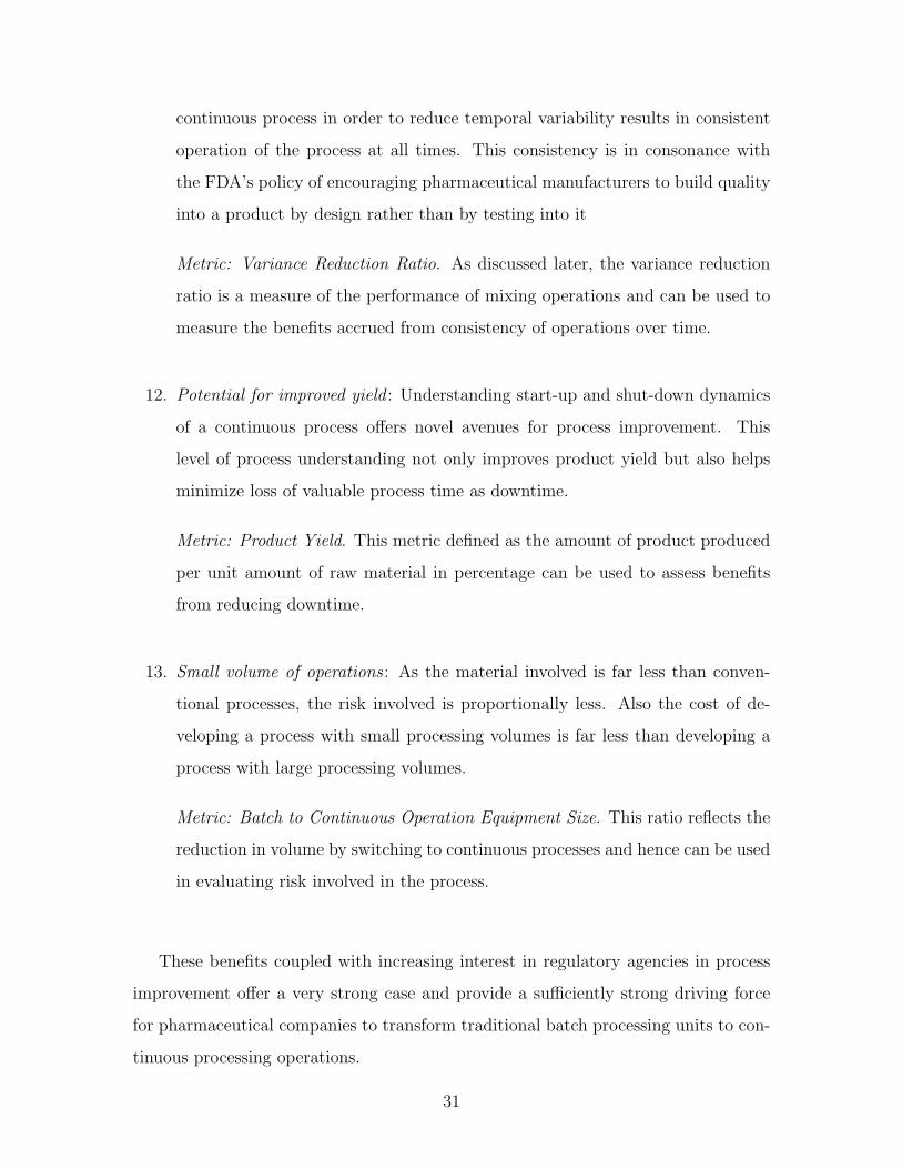
12. Potential for improved yield : Understanding start-up and shut-down dynamics
of a continuous process offers novel avenues for process improvement. This
level of process understanding not only improves product yield but also helps
minimize loss of valuable process time as downtime.
Metric: Product Yield. This metric defined as the amount of product produced
per unit amount of raw material in percentage can be used to assess benefits
from reducing downtime.
13. Small volume of operations : As the material involved is far less than conven-
tional processes, the risk involved is proportionally less. Also the cost of de-
veloping a process with small processing volumes is far less than developing a
process with large processing volumes.
Metric: Batch to Continuous Operation Equipment Size. This ratio reflects the
reduction in volume by switching to continuous processes and hence can be used
in evaluating risk involved in the process.
These benefits coupled with increasing interest in regulatory agencies in process
improvement offer a very strong case and provide a sufficiently strong driving force
for pharmaceutical companies to transform traditional batch processing units to con-
tinuous processing operations.
31
1.4 Powder Blending
Blending of powders is a crucial unit operation in many industries like the manufacture
of chemicals, construction materials, plastics and drugs. Batch blending has been in
use in a large number of processes especially when small volumes of materials are
processed; as a consequence there is a vast experience in handling powders in batches.
However, some high volume materials are often blended continuously. Instead of
debating which method of processing is better, one can view these two methods as
complementary process design choices that need to be made based on the economics
of the process aligned with appropriate quality specifications.
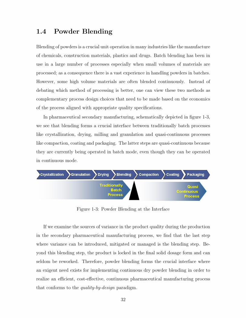
In pharmaceutical secondary manufacturing, schematically depicted in figure 1-3,
we see that blending forms a crucial interface between traditionally batch processes
like crystallization, drying, milling and granulation and quasi-continuous processes
like compaction, coating and packaging. The latter steps are quasi-continuous because
they are currently being operated in batch mode, even though they can be operated
in continuous mode.
Figure 1-3: Powder Blending at the Interface
If we examine the sources of variance in the product quality during the production
in the secondary pharmaceutical manufacturing process, we find that the last step
where variance can be introduced, mitigated or managed is the blending step. Be-
yond this blending step, the product is locked in the final solid dosage form and can
seldom be reworked. Therefore, powder blending forms the crucial interface where
an exigent need exists for implementing continuous dry powder blending in order to
realize an efficient, cost-effective, continuous pharmaceutical manufacturing process
that conforms to the quality-by-design paradigm.
32

1.5 Thesis Outline
This thesis begins with an extensive literature review of the published research work
on continuous dry powder blending in chapter 2. The literature review focuses on
the reported research and results on continuous blending achieved thus far, followed
by an analysis of areas where continuous blending phenomena can borrow ideas from
work on dry powder batch blending. Before presenting the conclusions on literature
review, this chapter also takes a peek at the various non-invasive analytical techniques
that were used to examine the quality of a powder mixture.
In chapter 3, The thesis goal is then discussed along with a proposed specfic
objectives and path of research. In chapter 4, the choices of the powder blending
systems, choices of powders, choices of process analytical techniques and the two
types of experiments that were performed on all the blenders and powders using the
analytical techniques are described in detail. The theories behind evaluating these
RTD and blending experiments are also described.
The experimental work on the Patterson-Kelley Zigzag R© blender and the analsis of
the data collected are then described in chapter 5. The results of these experiments are
described in chapter 6, where first the results from RTD experiments are described and
followed by the results from blending experiments. The effect of operational variables
on the blender performance is then described along with the effect of lubricant on
blending performance.
The experimental work on double helical ribbon blender and the analysis of the
data collected was described in chapter 7. Residence time distribution experiments
were performed with different combinations of excipients and APIs. The flow behavior
of powder in the ribbon blender is also described with the effect of fill weight on the
different operational parameters, fill weight, angle of incline and shaft rotation rate.
The effect of variance reduction ratio on the operational parameters and mainly mean
residence time is described and time period of disturbance is described in chapter 8.
The connection between microscopic properties and macroscopic phenomena in
continuous blending is described in chapter 9. The effect of particle size, cohesion
33

and shape are discussed. The effect of scale of scrutiny and the predictive capability
of blending models from residence time distributions are also discussed.
Finally, the path for future research in this growing area of pharmaceutical con-
tinuous processing is described in chapter 10, while chapter 11 focuses on developing
and applying a strategic framework for pharmaceutical manufacturing strategies be-
fore the conluding the thesis in chapter 12.
34

Chapter 2
Literature Review
The research on powder blending focused on developing a fundamental perspective
and aid predictive modeling of these processes and devices. Within this framework,
batch blending of powders received considerable attention compared to continuous
blending. This review reflects on the principles and knowledge accumulated over the
past half-century in the area of continuous powder blending.
Much of the initial research on continuous blending of powders focused on extend-
ing the principles of continuous liquid blending and teasing out the design principles
based on response-stimulus experiments. Though powder behavior was poorly un-
derstood from a fundamental standpoint, it might be expected that a number of the
principles behind powder blending in batch systems would play an important role
in continuous systems. For example, the mechanisms of convective mixing, diffusive
mixing and shear mixing would be present in continuous blending systems as well.
For example, convective mechanism or blending of powders due to bulk movement of
powder is a dominant mechanism in V and Y blenders. Diffusive mechanism of mix-
ing refers to the random movement of powders across slip planes or failure zones and
on the free exposed surface of the powder is a dominant mechanism in drum and agi-
tated blenders. Shear mechanism, which is predominant in pin mill and other milling
devices, results in mixing of powders from the agglomeration and de-agglomeration
of powders.
A batch blending system that can be run in continuous mode can be expected
35
to possess similar mixing mechanisms. This is because in such continuous blend-
ing systems, a net axial flow is superimposed on the existing batch system to yield
a continuous flow. We can, therefore, extend the studies on powder movement in
batch blenders and use this knowledge carefully in designing experimental studies on
continuous blending. Therefore, this review also examines the fundamental mixing
mechanism studies and their conclusions for batch blending systems with the idea of
finding areas of application of these concepts in continuous blending.
2.1 Prior Reviews
A previous review, by Williams [105], on continuous mixing of solids presented the
current thinking on the topic. A number of developments have occurred since then
and this review examines these developments as well. Also, this review differs from
previous reviews in that it emphasizes on applying principles of batch blending to
continuous blending. This review is organized into three parts. The first part details
the theoretical work that set the stage in understanding and characterizing continuous
blending. This theoretical background is of immense use in establishing design and
performance limits on continuous blenders as well as to develop process models for
continuous blending.
The main focus of the published literature was to study continuous blending in a
classical black box type analysis without giving much importance to the interactions
of the material in the blender. The second part illustrates the experimental studies
that were performed to understand continuous blending systems and to examine the
theory proposed. This part tries to extract some conclusions on a number of studies
on continuous blending. The third part examines the research on batch blending
and mixing mechanisms with the aim of identifying areas of possible complementary
exchange and use of ideas between batch and continuous blending. Our goal in this
chapter is to bring together the knowledge from over 50 publications and establish a
platform on which the attributes of continuous blending can be understood across a
wide range of applications.
36

2.2 Theoretical Developments
The earliest work on continuous blending addressed the assessment of the performance
of a continuous blender. Beaudry defined blender efficiency for continuous and semi-
continuous blenders based on the variance reduction ratio [5]. The variance reduction
ratio (VRR) is the ratio of the variance of the input stream to that of the output
stream of the blender and provides a key performance metric in continuous flow
systems. The variance of a stream is a measure of the spread of the composition of
the component of interest in that stream. Hence, the variance reflects the intensity
of segregation of the mixture in that stream and the VRR reflects the performance
of the blender in reducing this intensity of segregation. Clearly, we can see that a
higher VRR corresponds to better performance of the blender.
In the pharmaceutical industry, the acceptance of a good blend is usually based
on the relative standard deviation (RSD) of the concentration of the component of
interest in the blend, usually the active pharmaceutical ingredient (or API). A higher
variance reduction ratio in a blender gives a powder with lower variance at the output
and hence a blend with lower relative standard deviation. This connection between
the variance reduction ratio and the size of the blender will be discussed in detail
later.
2.2.1 Ideal Continuous Blender
The idea of ideal mixing as developed by Danckwerts [21, 22] was extended to free-
flowing non-segregating powders [106, 107]. It was shown that batch to batch vari-
ations can be reduced by feeding the batches semi-continuously to the blender [36].
The VRR in continuous blenders as derived by Danckwerts was derived as a limiting
case of the semi-continuous blender VRR where an infinitesimal amount of material
is simultaneously fed into and removed from the blender.
Based on the idea of the distribution of residence times in a blender, a model
was developed assuming that the objective of a blending process was to reduce the
output variance of the constituent component in the streams fed into the blender.
37

This variance reduction ratio defined by equation (2.1), was related to the feed char-
acteristics [22, 105, 106] by assuming an ideal blender with exponential decaying or
Poisson distribution of residence times. The feed was assumed to fluctuate with a fi-
nite correlation between two different times and the correlation was assumed to decay
in a geometric progression as given by equation (2.2) with increasing time of scrutiny.
V RR =σ2i
σ2o
= 1− τ · log a (2.1)
R(r) =cov(xt, xt+r)
var(xt)= ar (2.2)
where ‖a‖ < 1 is the serial correlation coefficient, is the standard deviation of the
concentration of a component of interest in the mixture, is the mean residence time
of the blender and subscript i is for input, o for output, t for time, r is the window
of observation. In order to describe the non-idealities in the blending process, the
residence time distribution (RTD) was modeled using delay and dead volume [107,
109], tanks in series [109] or dispersion models [1, 91, 96].
2.2.2 Non-Ideal Continuous Blender
Segregation of constituents in blending plays a very important role in powder blend-
ing. In order to characterize the homogeneity and structure of the blend at the output,
it is important to understand and assess the performance of the blender based on the
intensity and scale of segregation. While intensity of segregation is a measure of the
spread of the concentration of the component of interest in the mixture, the scale
of segregation reflects the correlation of the composition of that component in that
mixture (as a function of time for continuous systems and as a function of space for
batch systems).
Scale and intensity of segregation, therefore, describe the amount of unmixed
material within the mixture. A good mixture will have a small scale of segregation
and a low intensity of segregation (c.f. figure 2-1). The role of a mixer is to reduce
38

Figure 2-1: Scale and Intensity of Segregation
the scale of segregation and to lower the intensity of segregation. As the scale of
examination of the powder depicted in figure 2-1 varies, the observed variance changes
accordingly. This scale of examination, called scale of scrutiny [61, 62, 63, 72, 85, 88],
is an important experimental variable. Usually, the scale of scrutiny is determined
by the aim of the blending process. In pharmaceutical manufacturing, the scale of
scrutiny is usually chosen to be 3× the equivalent mass of the tablet or capsule.
Figure 2-2: Perfect and Random Mixtures
The best mixture that can be achieved by any physically realizable blender is the
random mixture shown in figure 2-2. Ghaderi [34] proved that the VRR in a continu-
ous blender was limited by that of a random mixture, first proposed by Weinekotter
39

and Reh [104], by variographic analysis. Therefore, an ideal blender cannot reduce
the variance below this limit. Also, it is clear that the structure of the two blends in
figure 2-3 is markedly different though the variances of both are the same. Clearly,
the second mixture has a different correlation or scale of segregation. Therefore, time
series analysis of the variances or variographic characterization and frequency domain
analysis of composition or power density spectrum analysis were used to determine
the intensity and scale of segregation during the blending process [34, 104].
Figure 2-3: Structurally Different Powder Blends
The general relation between the VRR and a general RTD, E(t), is given by
equation (2.3)
1
V RR= 2
∞∫t=0
∞∫τ=0
E(t)E(t+ τ)R(τ) dτ dt (2.3)
Also according to Danckwerts [22], the scale of segregation, Io is defined by equa-
tion (2.4).
Io =
∞∫τ=0
R(τ) dτ (2.4)
Weinektter and Reh [104] showed that the Fourier transform of the autocorrelation
40

function as in equation (2.5) could be employed to determine the scale and intensity
of segregation.
Gf (f) = 4
∞∫τ=0
R(τ) cos(2πfτ) dτ (2.5)
In the frequency domain, the area under the one-sided power density spectrum
equation (2.6), gave the intensity of segregation while the value at zero frequency
gave the scale of segregation given by equation (2.7).
σ2 =
∞∫0
Gf df (2.6)
I0 =Gf (f = 0)
4σ2(2.7)
This analysis was applied to understand the effect of the feeder fluctuations on
segregation. Two important conclusions that evolved from these developments are:
first, an ideal blender is constrained to reduce the variance to that of a random
mixture under ideal feeding conditions. For non-segregating, equal sized particles,
a random mixture is the mixture with the smallest attainable variance from any
physically realizable blending process [28]. As a result, an ideal powder blender
cannot reduce the variance beyond the random mixture limit for free-flowing non-
segregating powders. Second, an ideal blender is constrained in its performance to
smooth only high frequency fluctuations from the feeder. This means that an ideal
powder blender behaves as a low pass filter with the mean residence time as the time
constant or the inverse of the mean residence time as the cut-off frequency. Hence,
an ideal blender’s performance is a function of the feeder consistency.
Fokker-Planck equations (c.f. equation (2.8)) were used to model the dynamics of
mixing in a continuous rotary powder blender [48]. FPEs were written for each of the
component and were solved using void fraction of each component as the dependent
variable varying over time and space. The FPEs for the two components were coupled
41

at the exit of the blender by adjusting for the opening (or weir height). It was shown
that the ratio of the mean residence time to the time period of the fluctuation in the
feed is the most important parameter determining the variance reduction ratio.
∂C
∂t= −ν ∂C
∂z+D
∂2C
∂z2(2.8)
where C is the concentration of a component being mixed in the blender, ν is the
transport coefficient, D is the dispersion coefficient and z is the axial distance from
one end of the blender.
In a recent publication, Markov chains were applied to model continuous blending
of fine powders by Berthiaux et al., [6]. The continuous blender was assumed to
be made up of a series of well mixed states. The probability of material in a state
remaining in the same state in the next time step was ps. The probability of the
material in a state moving to the next state in the next time step was pf. The
probability of the material in a state moving to the previous state in the next time
step was pb. The ratio of pf/pb depends on the angle of the blades installed while
ps depends on the fill level of the mixture (or layer height). Obviously, these three
probabilities are exhaustive and hence add up to unity. Also, the exit of the material
out of the blender depended on the exit probability, w, which in turn depends on the
geometry and size of the outlet (weir height and area of opening). Simulations were
performed with sinusoidal feeding of one of the components. The general conclusions
from the simulations were that the frequency of the disturbance entering the blender
along with the mean residence time determines the variance reduction ratio. The
effect of the design of the exit of the blender (geometry and size) is significant in
continuous powder blender design and operation.
42

Tab
le2.
1:T
heo
reti
cal
Model
sfr
omL
iter
ature
Ob
ject
ive
Meth
od
Com
ments
Refs
.
Per
form
ance
ofco
n-
tinuou
sble
nder
s
Mas
sbal
ance
onth
eco
nti
nuou
s
ble
nder
An
index
ofp
erfo
rman
cefo
r
sem
i-co
nti
nuou
san
dco
nti
nuou
s
ble
nder
s
[5]
Char
acte
riza
tion
of
mix
ing
pro
cess
es
Mas
sbal
ance
onco
nti
nuou
s
ble
nder
s
Defi
nes
inte
nsi
tyan
dsc
ale
ofse
g-
rega
tion
and
scal
eof
scru
tiny
dis
-
cuss
ed
[22]
Per
form
ance
ofco
n-
tinuou
sble
nder
s
Res
pon
sest
imulu
sm
ethod
An
expre
ssio
nfo
rp
erfo
rman
ce
ofa
mix
erbas
edon
frac
tion
of
mix
erac
ting
idea
lly
was
der
ived
and
phen
omen
olog
ical
expla
na-
tion
sw
ere
not
pro
vid
ed
[106
]
Con
tinued
onN
ext
Pag
e...
43
Ob
ject
ive
Meth
od
Com
ments
Refs
.
Impro
vem
ent
over
bat
chble
ndin
g
Sta
tist
ical
Anal
ysi
sT
heo
reti
cal
per
form
ance
ofse
mi-
conti
nuou
sble
ndin
gop
erat
ion
was
der
ived
and
found
tob
e2
tim
esth
atof
abat
chble
nder
.
Mor
eove
r,ir
onin
gou
tof
the
bat
chto
bat
chva
riat
ions
reduce
s
the
volu
me
offa
iled
pro
duct
unit
s
consi
der
ably
[36]
Char
acte
rizi
ng
the
random
vari
atio
ns
in
able
nder
outp
ut
Pow
erden
sity
spec
trum
and
var-
iogr
aphic
anal
ysi
s
The
assu
mpti
onof
VR
Rof
aco
n-
tinuou
sble
nder
tob
eth
esu
mof
ara
ndom
bac
kgr
ound
ban
dlim
-
ited
whit
enoi
sean
da
reduct
ion
vari
ance
ofth
efe
edin
duce
dfluc-
tuat
ions
was
theo
reti
cally
and
ex-
per
imen
tally
just
ified
.
[34,
104]
Con
tinued
onN
ext
Pag
e...
44

Ob
ject
ive
Meth
od
Com
ments
Refs
.
Char
acte
riza
tion
of
ble
nder
per
form
ance
usi
ng
dis
per
sion
model
Sti
mulu
sre
spon
sean
alysi
s:R
TD
anal
ysi
s
Adis
per
sion
model
for
free
flow
ing
pow
der
sin
conti
nuou
s
ble
nder
sw
asdev
elop
edbas
ed
onth
eco
nti
nuum
appro
xim
atio
n.
This
appro
xim
atio
nre
lies
onth
e
diff
usi
onm
echan
ism
ofth
epar
ti-
cle
onth
efr
eesu
rfac
ean
dth
edi-
lati
onon
the
par
tof
the
mix
ture
due
toag
itat
ion
[91,
96]
Char
acte
riza
tion
of
ble
nder
per
form
ance
usi
ng
Fok
ker
Pla
nck
Model
Sti
mulu
sre
spon
sean
alysi
s:R
TD
anal
ysi
s
Fok
ker-
Pla
nck
equat
ions
wer
e
use
dto
det
erm
ine
the
outp
ut
conce
ntr
atio
ndis
trib
uti
onfo
r
aim
puls
ein
put
and
this
was
rela
ted
toth
ere
siden
ceti
me
dis
trib
uti
onan
dit
sst
atis
tica
l
mom
ents
[67]
Con
tinued
onN
ext
Pag
e...
45

Ob
ject
ive
Meth
od
Com
ments
Refs
.
Char
acte
riza
tion
of
ble
nder
per
form
ance
usi
ng
Fok
ker
Pla
nck
Model
Sti
mulu
sre
spon
sean
alysi
s:R
TD
anal
ysi
s
Fok
ker-
Pla
nck
equat
ions
wer
e
use
dto
des
crib
eth
era
ndom
mix
-
ing
ofp
owder
s.T
he
sam
eth
eory
was
use
dto
defi
ne
segr
egat
ion
kin
etic
sduri
ng
mix
ing
[93]
Char
acte
riza
tion
of
ble
nder
per
form
ance
usi
ng
Fok
ker
Pla
nck
Model
Sti
mulu
sre
spon
sean
alysi
s:R
TD
anal
ysi
s
Tw
oF
okke
r-P
lanck
equat
ions
wer
eso
lved
num
eric
ally
for
two
com
pon
ents
.O
ne
com
pon
ent
was
fed
sinuso
idal
lyto
contr
ol
the
dis
turb
ance
ente
ring
the
ble
nder
.R
atio
ofre
siden
ceti
me
top
erio
dof
osci
llat
ion
ofth
e
feed
dis
turb
ance
was
found
tob
e
crit
ical
par
amet
er
[48]
Con
tinued
onN
ext
Pag
e...
46

Ob
ject
ive
Meth
od
Com
ments
Refs
.
Ble
nder
Model
ing
us-
ing
Mar
kov
Chai
ns
Mar
kov
chai
ns
The
ble
nder
was
model
edas
a
Mar
kov
pro
cess
.T
he
tran
siti
on
pro
bab
ilit
ies
for
the
ble
nder
suse
d
by
(Wei
nek
’ott
eran
dR
eh[1
04])
was
use
din
det
erm
inin
gth
etr
an-
siti
onpro
bab
ilit
ym
atri
x.
The
de-
sign
ofth
eou
tlet
alon
gw
ith
resi
-
den
ceti
me
and
tim
ep
erio
dof
os-
cillat
ion
ofth
efe
edw
ere
found
to
be
crit
ical
par
amet
ers
[6]
End
ofT
able
47

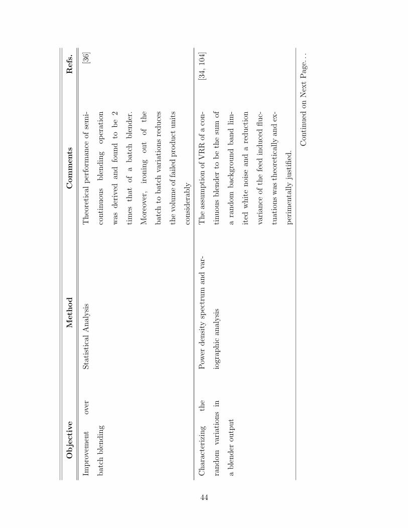
A list of the theoretical developments in the published literature is given in Ta-
ble 2.1. Attempts of using classical RTD models as mentioned before have been made
in a number of studies. As in the case of fluids, dispersion superimposed on plug-flow
was used to determine the profile of a tracer injected at the input. The profile was
solved for by using classic Danckwerts’ boundary conditions on the dispersion equa-
tion for plug flow. The resulting relation between the coefficient of dispersion and the
variance of the tracer as a function of distance from the input was used in determin-
ing the VRR [14, 91, 96]. These models work fairly well for non-cohesive powders.
However, concerns over their applicability for cohesive powders remain unanswered.
2.3 Studies on Continuous Powder Blending
A number of experimental studies were carried out on continuous blending systems.
However, none of these studies examined pharmaceutical powders or pharmaceutical
powder mixing closely.
2.3.1 Powders in Continuous Blending Studies
The published experimental studies on continuous powder blending fall into two broad
categories. One set was based on testing the applicability and validity of the theoreti-
cal developments on continuous blending while the other was aimed at characterizing
and understanding the performance of continuous powder blenders for different pow-
ders and look for patterns that could be used as generic design rules. Table 2.2 lists
the powders described in the literature under continuous blending. Free flowing non-
segregating type materials are the most common powders studied. A majority of the
powder systems were granular sand or silica with sugar or salt as tracer. Some of the
uncommon powders that were reported include chocolate, urania, thoria, zircon and
coal. The particle sizes of the powders investigated vary from as small as 0.5µm to as
large as 2cm. It is interesting to observe that pharmaceutical powders have not been
reported in continuous blenders.
48
2.3.2 Feeding in Continuous Blending Systems
As discussed before, a continuous blender’s performance is dependent on the feeding
characteristics. The intensity and scale of segregation was shown to be dependent
on the scale of scrutiny for powders. Scale of scrutiny also determines the feed ac-
curacy demanded. Therefore, feeding mechanism and monitoring techniques play a
substantial role in design and investigation of continuous blending systems. Table
2.3 makes a comparison between the feeding mechanism and the sampling and an-
alytical technique used in monitoring various experiments carried out in continuous
powder blending. Different powder feeding systems and their modes of operation
were described by Weinekotter and Gericke [103]. A continuous powder feeding sys-
tem consists of three distinct parts, the feeder unit, the measurement unit and the
control unit. The feeder unit produces the requisite volumetric or gravimetric flow of
the powder by screw, vibrating, rotary valve, belt, agitator, disc feeders. The mea-
surement unit measures the volume of flow from geometry and operating conditions
of the feeder or the weight of flow from direct measurement. The control unit controls
the feeder drive to regulate the feeding rate.
Three kinds of feeding systems were described by Weinekotter and Gericke [103]:
individual autonomous feeding, recipe feeding and proportional feeding. Individual
autonomous feeding systems control the feeding rates of each powder stream inde-
pendently. Recipe feeding systems maintain constant percentage proportions of the
ingredients but the overall volumetric flow rate is adjusted depending on disturbances.
Proportional feeding systems control the feeding rates based on one the flow rate of
the primary ingredient which acts as a master while the other controllers act as slaves.
The measurement and control system for feeding systems can be performed vol-
umetrically or gravimetrically. Two types of gravimetric feeding systems were re-
ported [103]. Weigh belt feeders operate with the powder flowing from a hopper on
to a belt and the weight measurement performed on the hopper or on the belt. Loss-
in-weight or differential feeders operate with two hoppers connected with a powder
volumetric flow device. The first hopper refilling the second till an upper limit is
49

reached. The second hopper, whose weight is monitored, then starts feeding contin-
uously via a screw feeder. As the weight of the powder in the second hopper falls
below a lower limit, the first hopper restarts its refilling operation.
Volumetric feeding was found to be less reliable than weigh feeding using a vi-
brated hopper delivering directly onto a moving belt on a weigh machine [41, 103].
Pulsed input was also used as a reliable experimental feeding technique [106]. It was
easy to introduce and control the fluctuations thus facilitating the study of blender
performance with the feeding mechanism.
50
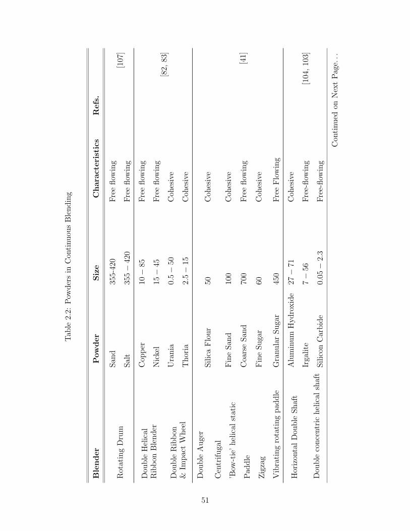
Tab
le2.
2:P
owder
sin
Con
tinuou
sB
lendin
g
Ble
nder
Pow
der
Siz
eC
hara
cteri
stic
sR
efs
.
San
d35
5-42
0F
ree
flow
ing
Rot
atin
gD
rum
Sal
t35
5−
420
Fre
eflow
ing
[107
]
Dou
ble
Hel
ical
Cop
per
10−
85F
ree
flow
ing
Rib
bon
Ble
nder
Nic
kel
15−
45F
ree
flow
ing
Dou
ble
Rib
bon
Ura
nia
0.5−
50C
ohes
ive
[82,
83]
&Im
pac
tW
hee
lT
hor
ia2.
5−
15C
ohes
ive
Dou
ble
Auge
rSilic
aF
lour
50C
ohes
ive
Cen
trif
uga
l
’Bow
-tie
’hel
ical
stat
icF
ine
San
d10
0C
ohes
ive
Pad
dle
Coa
rse
San
d70
0F
ree
flow
ing
[41]
Zig
zag
Fin
eSuga
r60
Coh
esiv
e
Vib
rati
ng
rota
ting
pad
dle
Gra
nula
rSuga
r45
0F
ree
Flo
win
g
Hor
izon
tal
Dou
ble
Shaf
tA
lum
inum
Hydro
xid
e27−
71C
ohes
ive
Irga
lite
7−
56F
ree-
flow
ing
[104
,10
3]
Dou
ble
conce
ntr
ichel
ical
shaf
tSilic
onC
arbid
e0.
05−
2.3
Fre
e-flow
ing
Con
tinued
onN
ext
Pag
e...
51

Ble
nder
Pow
der
Siz
eµm
Chara
cteri
stic
sR
efs
.
Rot
atin
gdru
mR
edan
dw
hit
eZ
eolite
pel
lets
(40%
Silic
aan
d
40%
Alu
min
a)
L=
3000
;D
=15
00F
ree
flow
ing
[96]
Rot
atin
gdru
mL
imes
tone
Vble
nder
Cop
per
40−
200
Fre
eflow
ing
[68,
70]
Plo
ugh
shar
em
ixer
Quar
tz
Dol
omit
e35
7F
ree
flow
ing
Dol
omit
e35
9F
ree
flow
ing
Dry
pow
der
335
Fre
eflow
ing
Bal
liti
ni
200
Fre
eflow
ing
Ric
eL
=50
00D
=20
00F
ree
flow
ing
Rot
atin
gD
rum
Lig
nit
e96
00F
ree
flow
ing
As
rep
orte
din
[91]
Zir
con
1700
Fre
eflow
ing
Coa
l27
00F
ree
flow
ing
Ilm
enit
e20
0F
ree
flow
ing
Ric
e20
00F
ree
flow
ing
Oat
s20
00F
ree
flow
ing
Con
tinued
onN
ext
Pag
e...
52

Ble
nder
Pow
der
Siz
eµm
Chara
cteri
stic
sR
efs
.
Pol
yst
yre
ne
H=
1900
L=
3600
Fre
eflow
ing
Soda
137
Fre
eflow
ing
San
d15
00F
ree
flow
ing
Coa
l50
0−
2000
0F
ree
flow
ing
Rot
atin
gD
rum
Pot
ato
star
ch15−
100
Fre
eflow
ing
As
rep
orte
din
[91]
Oat
groa
ts20
00F
ree
flow
ing
Coa
lw
ith
min
eral
6000−
1500
0F
ree
flow
ing
Gla
ssb
eads
3000
Fre
eflow
ing
Rot
atin
gD
rum
Mai
zest
arch
15C
ohes
ive
[48]
Cal
cium
Car
bon
ate
2C
ohes
ive
Co-
rota
ting
twin
scre
wC
hoco
late
10C
ohes
ive
[109
]
Plo
wsh
are
Cru
shed
Mai
ze37
0F
ree
flow
ing
[65,
66]
Mot
ionle
ssst
atic
Red
whea
tL
=64
50D
=29
00F
ree
flow
ing
[14]
Luci
te31
75−
5770
Fre
e-flow
ing
End
ofT
able
53

2.3.3 Process Monitoring of Continuous Blending
Early monitoring techniques for blending with one soluble component were based on
weighing the sample from a thief probe before and after dissolution. Some of the
recent advances in electronics encouraged more sophistication in monitoring experi-
mental powder blending. Power density spectrum analysis could be easily carried out
with electronic monitoring and modern day computing power. Optical imaging, opti-
cal reflectance, and positron emission and particle tracking (PEPT) were some of the
techniques reported for blend uniformity monitoring in continuous powder blending.
For powder systems where the tracer was optically different from the bulk, optical
laser and optical image techniques (reflectance based and color analysis based) were
used. This technique is amenable and reliable for online monitoring of powder blend-
ing if one of the components in the blend differs from the other constituents in color.
In the PEPT technique, gamma rays are emitted by a tracer particle followed by
capture of these rays in a positron camera. The position and velocity of the tracer
particle can then be reconstructed. This technique, however, is not amenable for
online monitoring as it involves usage of very special equipment and handling of ra-
dioactive tracers. A description of monitoring techniques in literature can be found
in tables 2.3 and 2.6.
54
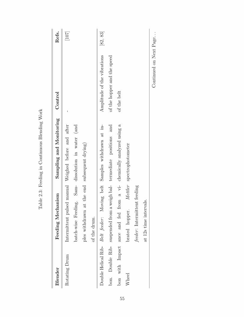
Tab
le2.
3:F
eedin
gin
Con
tinuou
sB
lendin
gW
ork
Ble
nder
Feedin
gM
ech
anis
mSam
pli
ng
and
Monit
ori
ng
Contr
ol
Refs
.
Rot
atin
gD
rum
Inte
rmit
tent
puls
edm
anual
bat
ch-w
ise
Fee
din
g.Sam
-
ple
sw
ithdra
wn
atth
een
d
ofth
edru
m.
Wei
ghed
bef
ore
and
afte
r
dis
solu
tion
inw
ater
(and
subse
quen
tdry
ing)
-[1
07]
Dou
ble
Hel
ical
Rib
-
bon
.D
ouble
Rib
-
bon
wit
hIm
pac
t
Whee
l
Bel
tfe
eder
:M
ovin
gb
elt
susp
ended
from
aw
eigh
bal
-
ance
and
fed
from
avi-
bra
ted
hop
per
.M
ettl
er
feed
er:
Inte
rmit
tent
feed
ing
at12
sti
me
inte
rval
s.
Sam
ple
sw
ithdra
wn
atin
-
term
edia
tep
osit
ions
and
chem
ical
lyan
alyze
dusi
ng
a
spec
trop
hot
omet
er
Am
plitu
de
ofth
evib
rati
ons
ofth
ehop
per
and
the
spee
d
ofth
eb
elt
[82,
83]
Con
tinued
onN
ext
Pag
e...
55
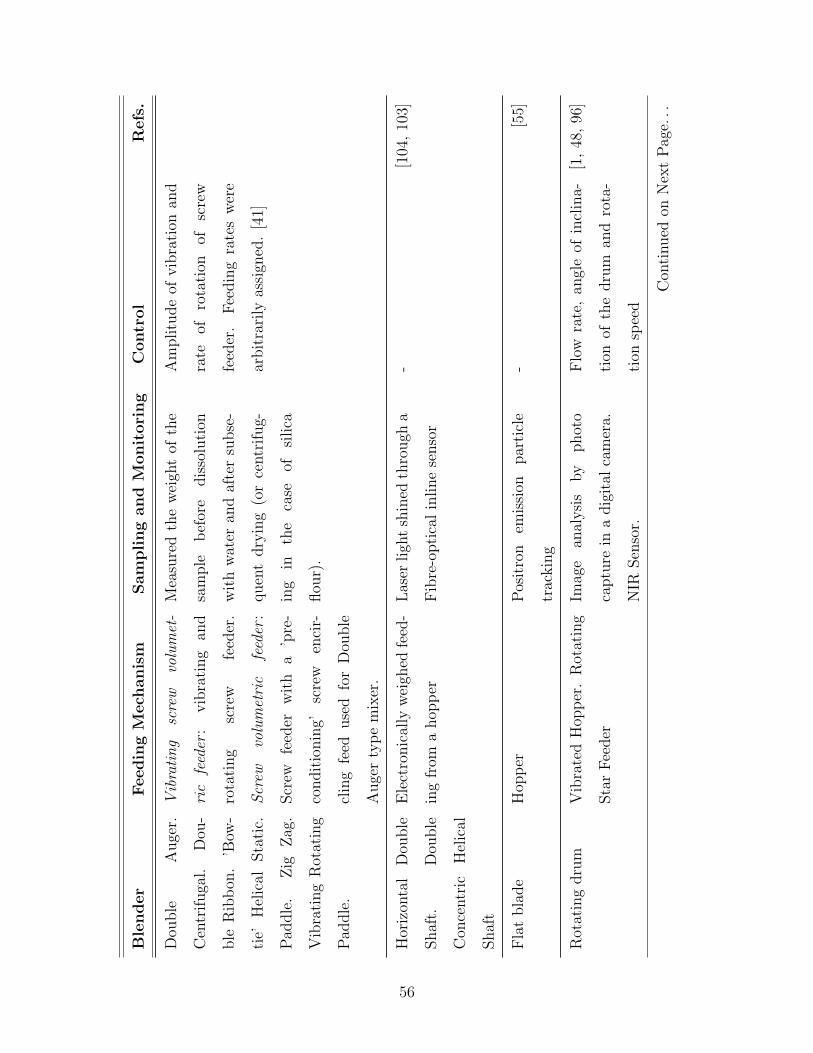
Ble
nder
Feedin
gM
ech
anis
mSam
pli
ng
and
Monit
ori
ng
Contr
ol
Refs
.
Dou
ble
Auge
r.
Cen
trif
uga
l.D
ou-
ble
Rib
bon
.’B
ow-
tie’
Hel
ical
Sta
tic.
Pad
dle
.Z
igZ
ag.
Vib
rati
ng
Rot
atin
g
Pad
dle
.
Vib
rati
ng
scre
wvo
lum
et-
ric
feed
er:
vib
rati
ng
and
rota
ting
scre
wfe
eder
.
Scr
ewvo
lum
etri
cfe
eder
:
Scr
ewfe
eder
wit
ha
’pre
-
condit
ionin
g’sc
rew
enci
r-
clin
gfe
eduse
dfo
rD
ouble
Auge
rty
pe
mix
er.
Mea
sure
dth
ew
eigh
tof
the
sam
ple
bef
ore
dis
solu
tion
wit
hw
ater
and
afte
rsu
bse
-
quen
tdry
ing
(or
centr
ifug-
ing
inth
eca
seof
silica
flou
r).
Am
plitu
de
ofvib
rati
onan
d
rate
ofro
tati
onof
scre
w
feed
er.
Fee
din
gra
tes
wer
e
arbit
rari
lyas
sign
ed.
[41]
Hor
izon
tal
Dou
ble
Shaf
t.D
ouble
Con
centr
icH
elic
al
Shaf
t
Ele
ctro
nic
ally
wei
ghed
feed
-
ing
from
ahop
per
Las
erligh
tsh
ined
thro
ugh
a
Fib
re-o
pti
cal
inline
senso
r
-[1
04,
103]
Fla
tbla
de
Hop
per
Pos
itro
nem
issi
onpar
ticl
e
trac
kin
g
-[5
5]
Rot
atin
gdru
mV
ibra
ted
Hop
per
.R
otat
ing
Sta
rF
eeder
Imag
ean
alysi
sby
phot
o
captu
rein
adig
ital
cam
era.
NIR
Sen
sor.
Flo
wra
te,
angl
eof
incl
ina-
tion
ofth
edru
man
dro
ta-
tion
spee
d
[1,
48,
96]
Con
tinued
onN
ext
Pag
e...
56
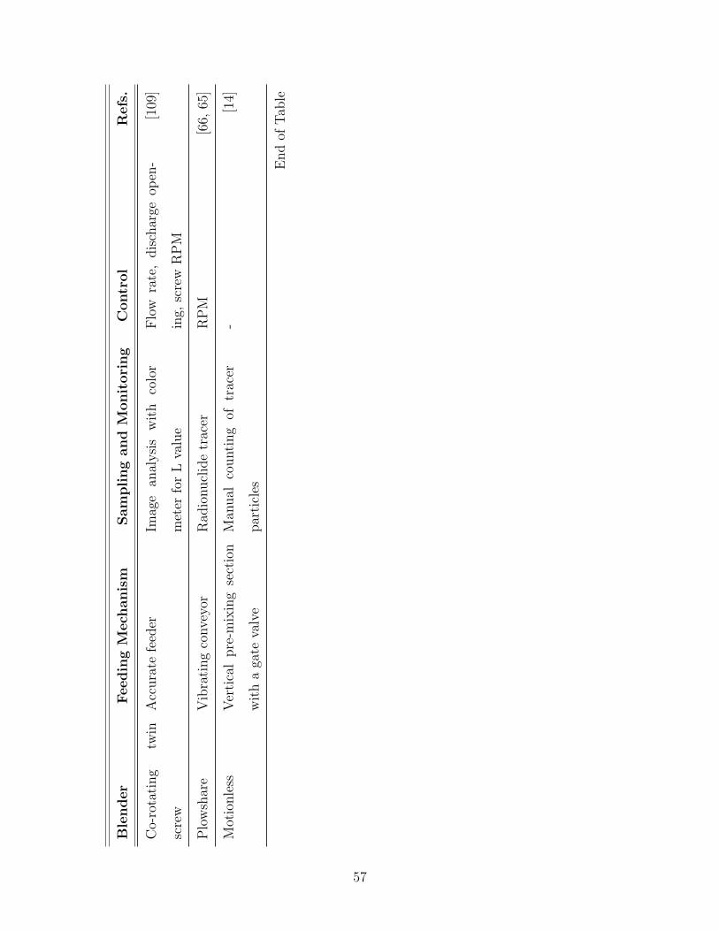
Ble
nder
Feedin
gM
ech
anis
mSam
pli
ng
and
Monit
ori
ng
Contr
ol
Refs
.
Co-
rota
ting
twin
scre
w
Acc
ura
tefe
eder
Imag
ean
alysi
sw
ith
colo
r
met
erfo
rL
valu
e
Flo
wra
te,
dis
char
geop
en-
ing,
scre
wR
PM
[109
]
Plo
wsh
are
Vib
rati
ng
conve
yor
Rad
ionucl
ide
trac
erR
PM
[66,
65]
Mot
ionle
ssV
erti
cal
pre
-mix
ing
sect
ion
wit
ha
gate
valv
e
Man
ual
counti
ng
oftr
acer
par
ticl
es
-[1
4]
End
ofT
able
57
Two kinds of analytical techniques are seen in powder blending research. The
first set of monitoring techniques is used for monitoring powder flow behavior in
blenders include techniques like positron emission and particle tracking and magnetic
resonance imaging. These complicated monitoring techniques usually are unfavorable
to be used in control systems for industrial application but are useful research tools
for understanding the fundamental behavior of powders in blenders. Another set of
analytical techniques are those that can be implemented as a process analytical tool in
an industrial manufacturing line process. These include technologies like light induced
fluorescence, near infrared spectrometry and optical reflectance. These are simpler
that the previous set of techniques and therefore can be applied in an industrial
process.
2.3.4 Process Control of Continuous Blending
Control strategies in many of these studies focused mainly on varying the operational
parameters such as flow rate, speed of the blender (RPM) and fill percent to control
the performance in the blender. None of these studies reported dynamic control of
the blend homogeneity. However, these studies did attempt to draw correlations
between the performance and these operational parameters. The usefulness of such
correlations is limited to the systems under consideration and is discussed later.
2.3.5 Experimental Studies on Continuous Blending
A summary of the conclusions from the investigations on continuous powder blenders
is tabulated in table 2.4. The qualitative and quantitative results from these stud-
ies show that, for non-cohesive systems, a response stimulus methodology explained
the behavior of the blenders fairly and also took into account the variations caused
by the feeding system. Some of the parameters reported in literature include frac-
tion of blender behaving ideally, delay, dead volume and dispersion coefficient. The
variation of these design parameters with operating parameters was either presented
graphically or by response surface methods. The fill percent proportional to the gate
opening in the blender of the rotating drum and twin screw blenders showed an op-
58
timum between 40-60% for many systems reported. For rotating drum blenders, the
dependence of the dispersion coefficient on the flow rate and rotational speed was pro-
portionally sub-linear. Correlations between dispersion coefficients, mean residence
times and the operational parameters like powder properties, blender geometry and
operating variables were proposed and were best fit curves for only the systems un-
der study and for certain regimes of flow in the drums (e.g. slow, avalanche flow).
Thus, extending these to other types of powders, blend geometries and regimes of
flow without considering the corresponding changes particle-particle interactions is
not justified. Further investigations must focus on developing a general correlation
between parameters of residence time distributions, operational parameters and par-
ticle properties. These correlations must be based on universal aspects of powder
behavior like forces between particles, segregation potential based on difference on
particle properties and finally the geometry of the blending system.
From the frequency domain analysis, it was shown that an ideal blender acted as a
low pass filter allowing the low frequency fluctuations from the feeder to pass through.
The structure of the mixture was predicted given the feeder auto-correlogram and
the RTD of the blender. The RTD was compared with a dispersion model and this
approach worked fairly well in explaining the observations.
In order to capture the dependence of agglomeration of cohesive powders, agglom-
erate particle size, Poole et al., [82, 83]. used in determining the random mixture
limit. De-agglomeration was another viable alternative that they investigated. It was
seen that de-agglomeration generally resulted in increased blend uniformity. How-
ever, no quantitative relations were reported relating the cohesive powder behavior
in this study. In order to deal with the uncertain behavior of cohesive powders some
studies have resorted to response-surface experimental methodology attempting to
explain the behavior of powders in continuous screw blenders. They performed ex-
periments with different operating points and tried to determine a linear or quadratic
dependence of mean residence time and fraction of the blender acting as a plug flow
device with operational parameters like gate opening (equivalent to fill percent inside
the blender), flow rate and so on. While these methods gave a functional relation
59

between the operational parameters and the behavior of the blender, these are sta-
tistically fitted functions and hence may not be extrapolated to other ranges of the
parameters.
The performance of commercial continuous blenders was evaluated for cohesive
powders [41]. Based on experiments on seven types of continuous blenders fed with
a vibrating hopper volumetric feeder, the blenders were ranked for cohesive powders
based on the variance of the exit stream. Harwood et al. concluded that centrifugal
blenders worked very well for cohesive powders while screw auger, paddle and ribbon
blenders gave above average performance. Use of particle emission and positron
tracking in determining the powder flow profiles and residence time were reported [53,
57, 54, 55, 56, 58]. Motionless blenders for free-flowing powders were studied [14, 39].
However, these blenders choke when cohesive powders are used [41].
Merz et al., [65, 66] used radionuclide tracers to investigate the residence time
distribution and used the dispersion model for calculating the effect of the shaft
rotation rate and influence of internal mixing geometries. It was pointed out that
by installing motionless weirs in the blender the dispersion coefficient was increased
significantly at high rotation rates. At low rotation rates, the dispersion coefficient
was hindered by the placement of weirs. The mean residence time was found to reach
a maximum at 1.4 times the critical rotation rate (The critical rotation rate being
defined as the rate at which the gravitational force is balanced by the centrifugal
force).
60
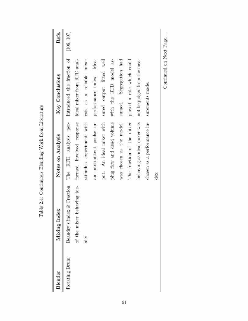
Tab
le2.
4:C
onti
nuou
sB
lendin
gW
ork
from
Lit
erat
ure
Ble
nder
Mix
ing
Index
Note
son
Analy
sis
Key
Concl
usi
on
sR
efs
.
Rot
atin
gD
rum
Bea
udry
’sin
dex
&F
ract
ion
ofth
em
ixer
beh
avin
gid
e-
ally
The
RT
Dan
alysi
sp
er-
form
edin
volv
edre
spon
se
stim
ulu
sex
per
imen
tw
ith
anin
term
itte
nt
psu
lse
in-
put.
An
idea
lm
ixer
wit
h
plu
gflow
and
dea
dvo
lum
e
was
chos
enas
the
model
.
The
frac
tion
ofth
em
ixer
beh
avin
gas
idea
lm
ixer
was
chos
enas
ap
erfo
rman
cein
-
dex
Intr
oduce
dth
efr
acti
onof
idea
lm
ixer
from
RT
Dan
al-
ysi
sas
are
liab
lem
ixer
per
form
ance
index
.M
ea-
sure
dou
tput
fitt
edw
ell
wit
hth
eR
TD
model
as-
sum
ed.
Seg
rega
tion
had
pla
yed
aro
lew
hic
hco
uld
not
be
judge
dfr
omth
em
ea-
sure
men
tsm
ade.
[106
,10
7]
Con
tinued
onN
ext
Pag
e...
61
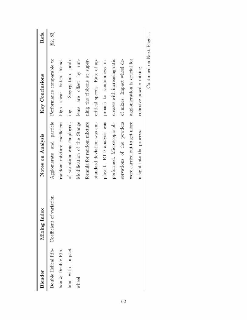
Ble
nder
Mix
ing
Index
Note
son
Analy
sis
Key
Concl
usi
on
sR
efs
.
Dou
ble
Hel
ical
Rib
-
bon
&D
ouble
Rib
-
bon
wit
him
pac
t
whee
l
Coeffi
cien
tof
vari
atio
nA
gglo
mer
ate
and
par
ticl
e
random
mix
ture
coeffi
cien
t
ofva
riat
ion
was
emplo
yed.
Modifi
cati
onof
the
Sta
nge
form
ula
for
random
mix
ture
stan
dar
ddev
iati
onw
asem
-
plo
yed.
RT
Dan
alysi
sw
as
per
form
ed.
Mic
rosc
opic
ob-
serv
atio
ns
ofth
ep
owder
s
wer
eca
rrie
dou
tto
get
mor
e
insi
ght
into
the
pro
cess
.
Per
form
ance
com
par
able
to
hig
hsh
ear
bat
chble
nd-
ing.
Seg
rega
tion
pro
b-
lem
sar
eoff
set
by
run-
nin
gth
eri
bb
ons
atsu
per
-
crit
ical
spee
ds.
Rat
eof
ap-
pro
ach
tora
ndom
nes
sin
-
crea
ses
wit
hin
crea
sing
rati
o
ofm
ixes
.Im
pac
tw
hee
lde-
aggl
omer
atio
nis
cruci
alfo
r
cohes
ive
pow
der
mix
ing
[82,
83]
Con
tinued
onN
ext
Pag
e...
62

Ble
nder
Mix
ing
Index
Note
son
Analy
sis
Key
Concl
usi
on
sR
efs
.
1.D
ouble
Auge
r
2.C
entr
ifuga
l
3.D
ouble
Rib
-
bon
4.’B
ow-t
ie’
He-
lica
lSta
tic
5.P
addle
6.Z
igZ
ag
7.V
ibra
ting
Rot
atin
g
Pad
dle
1.F
ract
ion
ofon
eof
the
pow
der
mat
eria
ls
2.Sta
ndar
ddev
iati
on
over
ase
tof
sam
ple
s
1.E
mer
gence
pro
file
sof
the
conce
ntr
atio
ns
as
frac
tion
sw
ere
plo
tted
2.M
ixer
sw
ere
ranke
din
the
order
ofin
crea
sing
stan
dar
ddev
iati
ons
for
cohes
ive-
cohes
ive,
cohes
ive-
free
flow
-
ing
and
free
-flow
ing
free
-flow
ing
pow
der
syst
ems
resp
ecti
vely
The
dou
ble
auge
r,vib
rati
ng
rota
ting
pad
dle
and
dou
ble
ribb
onble
nder
sw
ere
inth
e
mid
toupp
erp
erfo
rman
ce
range
for
mos
tp
owder
s.
The
dou
ble
hel
ical
stat
ic
mix
erch
oked
for
cohes
ive
pow
der
s.T
he
centr
ifuga
l
mix
erp
erfo
rmed
wel
lfo
r
cohes
ive
syst
ems.
Zig
-zag
ble
nder
isunsu
itab
lefo
rco
-
hes
ive
segr
egat
ing
syst
ems.
[41]
Con
tinued
onN
ext
Pag
e...
63

Ble
nder
Mix
ing
Index
Note
son
Analy
sis
Key
Concl
usi
on
sR
efs
.
1.H
oriz
onta
l
Dou
ble
Shaf
t
2.D
ouble
Con
-
centr
icH
eli-
cal
Shaf
t
1.In
tensi
tyof
segr
ega-
tion
from
vari
ance
2.Sca
leof
segr
egat
ion
from
corr
elat
ion
func-
tion
3.V
aria
nce
reduct
ion
ra-
tio
VR
R
Fro
mth
eR
TD
anal
ysi
s,th
e
inte
nsi
tyof
segr
egat
ion
(or
vari
ance
)is
calc
ula
ted.
The
scal
eof
segr
egat
ion
isca
l-
cula
ted
from
the
area
un-
der
the
curv
eof
the
pow
-
der
den
sity
spec
trum
.T
he
VR
Ris
calc
ula
ted
and
plo
t-
ted
asa
funct
ion
ofth
eB
o-
den
stei
nnum
ber
(als
oth
e
Pec
let
num
ber
)an
dth
ep
e-
riod
offluct
uat
ion
inth
e
feed
.
Aco
nti
nuou
sm
ixer
can
dam
pen
the
dis
turb
ance
s
that
are
only
inth
ehig
h
freq
uen
cyra
nge
(hen
ceac
t-
ing
asa
low
pas
sfilt
er).
The
tim
ep
erio
dof
dis
tur-
ban
cem
ust
be
less
than
the
resi
den
ceti
me
ofth
e
mix
er.
Opti
miz
atio
nof
feed
ing
syst
emby
allo
win
g
only
hig
hfr
equen
cydis
tur-
ban
ces
thro
ugh
the
feed
eris
anes
senti
alpar
tof
mix
er
des
ign.
[104
,10
3]
Con
tinued
onN
ext
Pag
e...
64

Ble
nder
Mix
ing
Index
Note
son
Analy
sis
Key
Concl
usi
on
sR
efs
.
Fla
tbla
de
Non
eF
low
pat
hs
wer
ege
ner
ated
exp
erim
enta
lly
and
qual
ita-
tive
des
crip
tion
ofth
em
ix-
ing
phen
omen
onw
asgi
ven.
PE
PT
can
be
use
dto
study
the
flow
pat
tern
san
dre
si-
den
ceti
me
dis
trib
uti
ons
of
pow
der
sin
conti
nuou
sm
ix-
ers.
[55]
Rot
atin
gdru
mD
isp
ersi
onco
effici
ent
The
resp
onse
toa
trac
er
intr
oduce
din
the
feed
is
trac
ked
and
the
outp
ut
is
sub
ject
edto
resi
den
ceti
me
anal
ysi
s.D
isp
ersi
onco
effi-
cien
tis
calc
ula
ted
by
fitt
ing
anax
ial
dis
per
sion
model
toth
eex
per
imen
tal
obse
r-
vati
ons.
RT
Dcu
rves
for
vari
ous
flow
rate
san
dat
vari
ous
sam
pling
poi
nts
alon
gth
e
lengt
hof
the
dru
mw
ere
re-
por
ted.
The
shap
esof
the
RT
Dar
ese
lf-s
imilar
(non
-
segr
egat
ing
par
ticl
es).
Var
i-
atio
nof
dis
per
sion
coeffi
-
cien
tw
ith
flow
rate
,R
PM
and
incl
inat
ion
angl
ew
as
rep
orte
d.
[96]
Con
tinued
onN
ext
Pag
e...
65

Ble
nder
Mix
ing
Index
Note
son
Analy
sis
Key
Concl
usi
on
sR
efs
.
Rot
atin
gdru
mD
isp
ersi
onco
effici
ent
PE
PT
was
use
dto
trac
kth
e
par
ticl
esan
ddis
per
sion
co-
effici
ent
for
bat
hc
mix
ing
in
adru
mw
asca
lcula
ted.
Dis
-
per
sion
coeffi
cien
tsfo
rro
-
tati
ng
dru
mm
ixin
gof
other
par
ticl
esy
stem
sre
por
ted
else
wher
ew
ere
calc
ula
ted.
Cor
rela
tion
sfr
omlite
ratu
re
for
dis
per
sion
coeffi
cien
t
wer
ere
por
ted
asa
funct
ion
offlow
rate
,ge
omet
ryof
the
dru
m,
par
ticl
esi
ze,
angl
eof
incl
inat
ion
dy-
nam
ican
gle
ofre
pos
ean
d
rota
tion
alsp
eed.
Anew
corr
elat
ion
for
bot
hbat
ch
and
conti
nuou
sdis
per
sion
was
dev
elop
edfr
omex
-
per
imen
tal
dat
aof
seve
ral
auth
ors.
[91]
Con
tinued
onN
ext
Pag
e...
66
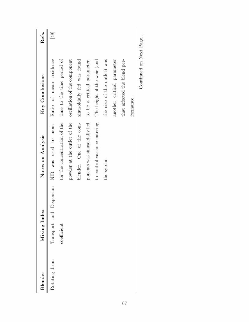
Ble
nder
Mix
ing
Index
Note
son
Analy
sis
Key
Concl
usi
on
sR
efs
.
Rot
atin
gdru
mT
ransp
ort
and
Dis
per
sion
coeffi
cien
t
NIR
was
use
dto
mon
i-
tor
the
conce
ntr
atio
nof
the
pow
der
atth
eou
tlet
ofth
e
ble
nder
.O
ne
ofth
eco
m-
pon
ents
was
sinuso
idal
lyfe
d
toco
ntr
olva
rian
ceen
teri
ng
the
syte
m.
Rat
ioof
mea
nre
siden
ce
tim
eto
the
tim
ep
erio
dof
osci
llat
ion
ofth
eco
mp
onen
t
sinuso
idal
lyfe
dw
asfo
und
tob
ea
crit
ical
par
amet
er.
The
hei
ght
ofth
ew
eir
(and
the
size
ofth
eou
tlet
)w
as
anot
her
crit
ical
par
amet
er
that
affec
ted
the
ble
nd
per
-
form
ance
.
[48]
Con
tinued
onN
ext
Pag
e...
67

Ble
nder
Mix
ing
Index
Note
son
Analy
sis
Key
Concl
usi
on
sR
efs
.
Co-
rota
ting
twin
scre
w
-R
esid
ence
tim
ean
alysi
s
from
was
hou
tex
per
imen
t
was
per
form
ed.
Del
ay
and
dea
dvo
lum
em
odel
and
tanks
inse
ries
model
wer
euse
din
expla
inin
g
the
exp
erim
enta
lre
sult
s.
Res
pon
sesu
rfac
ean
alysi
s
was
per
form
edon
the
effec
t
offe
edra
tes
and
RP
M
onre
siden
ceti
me
and
gate
open
ing
onfr
acti
onal
tubula
rity
.
The
mix
erco
mpri
sed
of
forw
ard
conve
yin
g,non
-
conve
yin
gan
dre
vers
ese
c-
tion
s.T
he
tanks
inse
-
ries
model
was
fitt
edw
ith
one
par
amet
er(n
um
ber
of
tanks
fixed
).Sta
tist
ical
in-
fluen
ces
offe
edra
tean
d
scre
wR
PM
onm
ean
res-
iden
ceti
me
and
ofga
te
open
ing
onfr
acti
onal
tubu-
lari
tyw
asob
serv
ed.
Are
-
spon
sesu
rfac
em
odel
was
use
dto
expla
inth
ere
sult
s.
Non
-dim
ensi
onal
RT
Dw
as
iden
tica
lfo
rhig
han
dlo
w
feed
rate
case
s.
[109
]
Con
tinued
onN
ext
Pag
e...
68

Ble
nder
Mix
ing
Index
Note
son
Analy
sis
Key
Concl
usi
on
sR
efs
.
Plo
wsh
are
Dis
per
sion
coeffi
cien
tR
esid
ence
tim
ean
aly-
sis
usi
ng
radio
nucl
ide
trac
er.D
isp
ersi
onm
odel
for
mix
ing
was
use
d.
RP
M
was
the
only
oper
atio
nal
vari
able
chan
ged
duri
ng
the
exp
erim
ent.
Eff
ect
of
pre
sence
ofin
tern
alw
eirs
was
exam
ined
Diff
eren
tplo
wco
nfigu
ra-
tion
sga
vediff
eren
tm
ean
resi
den
ceti
mes
and
stan
-
dar
ddev
iati
ons.
The
dis
-
per
sion
coeffi
cien
tin
the
pre
sence
ofin
tern
alw
eir
was
hig
her
than
that
init
s
abse
nce
only
atve
ryhig
h
rota
tion
rate
s.T
he
loca
tion
ofth
ein
tern
alw
eir
was
the
poi
nt
wher
eth
ere
siden
ce
tim
edis
trib
uti
onch
ange
d
its
shap
e.T
he
mea
nre
s-
iden
ceti
me
had
am
axi-
mum
ata
par
ticu
lar
rota
-
tion
rate
,ab
ove
the
crit
i-
cal
rota
tion
alra
te.
Inth
e
pre
sence
ofw
eirs
,th
em
ean
resi
den
ceti
me
had
am
axi-
mum
atm
uch
alo
wer
rota
-
tion
rate
.
[66,
65]
Con
tinued
onN
ext
Pag
e...
69

Ble
nder
Mix
ing
Index
Note
son
Analy
sis
Key
Concl
usi
on
sR
efs
.
Mot
ionle
ssD
isp
ersi
onco
effici
ent
Res
iden
ceti
me
anal
ysi
s
from
impuls
etr
acer
ex-
per
imen
tw
asco
nduct
ed.
Dis
per
sion
model
was
use
d
toex
pla
inth
ere
sult
s.H
old
up
tim
esfo
rfo
rva
riou
s
wei
ghts
ofpar
ticl
esw
as
rep
orte
d
Dis
per
sion
model
expla
ins
the
mix
ing
offr
ee-fl
owin
g
par
ticl
esin
mot
ionle
ssm
ix-
ers.
The
rela
tion
bet
wee
n
appar
ent
linea
rve
loci
tyan
d
dis
per
sion
was
inve
stig
ated
and
was
found
toin
crea
se
wit
hlinea
rve
loci
tyin
a
non
-lin
ear
man
ner
.T
he
num
ber
ofm
ixin
gel
emen
ts
(hel
ices
)in
crea
sed
the
dis
-
per
sion
coeffi
cien
t.
[14]
End
ofT
able
70
2.4 Research on Continuous and Batch Blending
As discussed in the introduction, powder blending has predominantly been a batch
process both in practice and research. These research efforts, on batch blenders that
can operate in continuous mode also, could prove valuable in understanding the be-
havior of powders in continuous mode. An attempt to understand how to supplement
continuous blending research from batch blending research would be supported by re-
viewing literature on batch blending. As many reviews tabulated in table 2.5 have
appeared before in literature, we chose not to include this in this review.
A number of reviews [28, 29, 61, 62, 63, 72, 85, 88, 102] focus on the various mixing
indices in use in industry and research, the mechanisms of mixing, the directions that
research had taken at the time of the review and some empirical rules to choose and
design blenders. Weidenbaum [102] reviewed about 75 papers before 1960 while Fan
et al., [28] reviewed over 200 papers in 1970 in their review. Though the number
of published papers in this area has not grown phenomenally, a shift in the areas of
emphasis is visible. The earlier reviews [28, 102] detailed the state of the knowledge
on blending like empirical kinetic equations, computer simulations of the stochastic
blending process, the selection criteria for blenders. The later reviews [29, 61, 62,
63, 72, 85, 88] emphasized fluidized beds, contact number based indices and the
concept of ordered mixing for cohesive powders. The series of reviews on solid and
liquid blending [61, 62, 63, 72, 88] detailed the blending equipment in the agricultural
industry. Williams reviewed the continuous blending literature and presented the
theoretical analysis discussed previously [105].
As noted earlier, blenders that can operate in both batch and continuous modes
can be expected to have similar powder behavior. Therefore, an understanding of the
mixing mechanisms in these batch blenders would, at least qualitatively, give some
guiding principles e.g. the effect of blades on powders, the effect of geometry of the
blender and the powder-powder and powder-wall interactions for designing continuous
blending systems.
71

Tab
le2.
5:P
ast
revie
ws
onP
owder
Ble
ndin
g
Focu
sT
yp
eM
ixers
Ref.
toC
onti
nuous
Ble
ndin
gR
efs
.
Rev
iew
oflite
ra-
ture
onso
lids
mix
-
ing
from
1958
-
1970
.C
atal
ogu-
ing
mix
ing
indic
es,
mix
ing
par
amet
ers,
rate
law
s,m
ixer
se-
lect
ion
crit
eria
and
sim
ula
tion
sin
mix
-
ing
rese
arch
Bat
chan
dco
n-
tinuou
s
Rib
bon
,F
low
,C
ircu
lati
on,
Gra
vit
y,C
entr
ifuga
l,M
o-
tion
less
Lit
tle
emphas
ison
conti
n-
uou
sm
ixin
g.A
list
ing
ofge
ner
alcr
iter
iafo
rse
-
lect
ing
mix
ers
was
com
-
piled
.Sol
ids
han
dling
pro
b-
lem
sw
ere
hig
hligh
ted
[28]
Con
tinued
onN
ext
Pag
e...
72

Focu
sT
yp
eM
ixers
Ref.
toC
onti
nuous
Ble
ndin
gR
efs
.
Con
tinuou
sm
ixin
g
ofso
lids
Bat
chan
dco
n-
tinuou
s
Dru
m,
Rib
bon
Mat
hem
atic
alan
alysi
sof
stim
ulu
s-re
spon
sean
alysi
s
for
conti
nuou
sm
ixer
was
give
n.
Qual
itat
ive
com
par
i-
son
bet
wee
nco
nti
nuou
san
d
bat
chm
ixer
sfo
rp
owder
s
was
mad
e
[105
]
Con
tinued
onN
ext
Pag
e...
73

Focu
sT
yp
eM
ixers
Ref.
toC
onti
nuous
Ble
ndin
gR
efs
.
Pow
der
mix
ing
mec
han
ism
s
Bat
chB
laded
,P
addle
,F
ludiz
ed
bed
Dep
enden
ceof
pow
der
ten-
sile
stre
ngt
hon
the
form
a-
tion
offa
ilure
zones
was
des
crib
ed.
Con
vect
ive
ef-
fect
son
flow
ofp
owder
over
bla
des
and
reci
rcula
-
tion
ofp
owder
over
the
bla
des
was
dis
cuss
ed.
Inte
r-
par
ticl
ep
erco
lati
onan
ddif
-
fusi
vem
ixin
gm
echan
ism
s
wer
edes
crib
ed.
An
exte
n-
sion
ofth
ean
alysi
sof
mix
-
ing
mec
han
ism
toco
hes
ive
and
adhes
ive
syst
ems
was
qual
itat
ivel
ym
ade.
[9,
10,
11,
46,
53,
57]
Con
tinued
onN
ext
Pag
e...
74

Focu
sT
yp
eM
ixers
Ref.
toC
onti
nuous
Ble
ndin
gR
efs
.
Lit
erat
ure
surv
ey
onp
owder
mix
ing
Bat
chan
dC
on-
tinuou
s
-E
xte
nsi
velite
ratu
resu
rvey
and
com
pre
hen
sive
clas
si-
fied
list
of65
0re
fere
nce
sin
Pow
der
mix
ing
bef
ore
1975
[16]
Rev
iew
onth
e
met
hods
ofm
ixer
des
ign
and
geom
e-
trie
s
Bat
chG
ravit
yfo
rce,
Pel
let,
Nau
-
tam
ix,
pneu
mat
ic,
fluid
ized
bed
,si
lo
Char
acte
rize
sble
nder
sde-
pen
din
gon
the
dom
inan
t
forc
eof
mix
ing
-gr
av-
ity,
push
and
centr
ifuga
l.
Know
ledge
arou
nd
mix
ing
tim
esan
dp
ower
requir
e-
men
tsth
atgo
into
mix
er
des
ign
are
dis
cuss
ed.
The
role
offr
icti
onal
forc
esin
the
wor
kdon
eon
mix
ing
is
also
dis
cuss
ed.
[69]
Con
tinued
onN
ext
Pag
e...
75
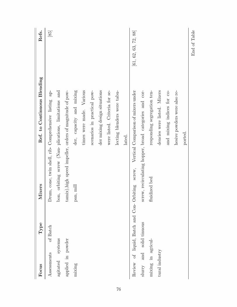
Focu
sT
yp
eM
ixers
Ref.
toC
onti
nuous
Ble
ndin
gR
efs
.
Ass
essm
ents
of
agit
ated
syst
ems
applied
inp
owder
mix
ing
Bat
chD
rum
,co
ne,
twin
shel
l,ri
b-
bon
,or
bit
ing
scre
w(N
au-
tam
ix),
hig
hsp
eed
imp
elle
r,
pan
,m
ill
Com
pre
hen
sive
list
ing
ap-
plica
tion
s,lim
itat
ions
and
order
sof
mag
nit
ude
ofp
ow-
der
,ca
pac
ity
and
mix
ing
tim
esw
ere
mad
e.V
ario
us
scen
ario
sin
pra
ctic
alp
ow-
der
mix
ing
des
ign
situ
atio
ns
wer
elist
ed.
Cri
teri
afo
rse
-
lect
ing
ble
nder
sw
ere
tabu-
late
d.
[85]
Rev
iew
ofliquid
,
slurr
yan
dso
lid
mix
ing
inag
ricu
l-
tura
lin
dust
ry
Bat
chan
dC
on-
tinuou
s
Orb
itin
gsc
rew
,V
erti
cal
scre
w,
reci
rcula
ting
hop
per
,
fluid
ized
bed
Com
par
ison
ofm
ixer
sunder
bro
adca
tego
ries
and
cor-
resp
ondin
gse
greg
atio
nte
n-
den
cies
wer
elist
ed.
Mix
ers
and
mix
ing
indic
esfo
rco
-
hes
ive
pow
der
sw
ere
also
re-
por
ted.
[61,
62,
63,
72,
88]
End
ofT
able
76

2.4.1 Powder Kinematics and Dynamics
Bridgwater [9, 10] discussed the various blending mechanisms in a batch blender and
the influence of particle and blender properties on them. It was shown that slip planes
or failure zones are formed when a blade moves in the powder. The creation of these
zones generates the degrees of freedom for the powder to move in bulk (convection)
and for particles to randomly move across these zones (diffusion). Some effort on
predicting slip planes will be discussed later. However, it was suggested that in
a fundamental mathematical model of a mixer, the mean failure zone height and
spacing measured in the same direction would be the characteristic length scales.
The formation of slip planes in convective mixers was shown to be a crucial step in
the process of blending. Novosad et al., [73, 74, 75, 76, 77] attempted to theoretically
predict the slip planes (and the accompanying failure zones) for non-segregating,
free-flowing powders. A blade rotating in a bed of powder was visually examined
from outside and the slip planes were predicted using classical powder mechanical
constructions. It was reported that theoretical predictions were possible to the zones
adjoining and close to the blade (in the fore and the hind). For far away zones,
the shape of the slip planes could not be predicted accurately. A state of limiting
equilibrium was assumed to exist with an active lateral pressure and inertial forces
were neglected. This assumption implied that the static and dynamic slip planes
would be of the same shape. With the knowledge of these planes, the shear stress
on the blade was also predicted using geometrical methods. The results agreed with
analytical Mohr’s circle method very closely. The theoretical stresses were then used
to develop correlations between the shaft torque on the powder as a function of
the geometry of the shaft, the properties of the granular material and wall, and
the position of the blade. The correlation developed showed fair agreement with
experiments.
Muller et al., studied the effect of internal mixing elements on blending [68, 70]. In
the same studies, the effect or rotation rate of blending elements, fill volume, particle
size distribution of tracer and bulk powder were also studied. The effect of torque and
77
work of mixing powders were examined for different internal elements. In a review,
the principles of batch mixer design and geometry were studied and correlations for
operational parameters and mixer performance indicators were reported for different
types of mixer geometries [69],
Cooker and Nedderman [19, 18] reported a theoretical analysis of powder dynamics
in a a more complicated geometry of the vertical helical ribbon agitator (HRA). In a
more recent study, the torque on high shear impellers was theoretically predicted [49].
They also experimentally verified and found that their model represented the torque
behavior fairly well. Extensions of these theoretical methods for cohesive powders
were not found. However, a model by Kocova and Pilpel [50] showed that principle
of corresponding states could be applied for predicting the tensile stresses in cohesive
powders. The tensile stresses in cohesive powders were related to the inter-particle
distances and the surface asperities of the powder.
A series of related studies on blending mechanisms using positron emission parti-
cle tracking gave an insight into the complex nature of interactions that occur inside
the blender. PEPT technique was used to study the powder movement profiles (ra-
dial and angular displacement and velocities) in various blenders (ploughs, bars and
agitators) [12, 46, 53, 57, 54, 55, 56, 58]. The position of the tracer at different times
inside the blender was used in estimating particle movement parameters like the mean
radial displacement and axial dispersion coefficient for different blender operational
variables. As these parameters were calculated from basic particle movement exper-
iments, these hold great value in characterizing the efficacy of the blender mixing
elements in the absence of theoretical models. Also, these experiments predicted the
occupancy of the tracer at different points of the blender, thereby giving important
information on deposits and dead volumes inside the blender. Using the movement
of particles, axial dispersion coefficients and mean radial displacements were deter-
mined from first hand experimental information. These investigations therefore are
important in independently determining axial dispersion coefficient rather than from
parameter fitting in residence time distribution experiments. Even though these stud-
ies have been performed on batch blenders, there are some ongoing efforts [53] to
78

implement this technique in understanding continuous blending systems.
Magnetic resonance imaging (MRI) was used by many authors in characterizing
the segregation of granules in rotating drum [42, 43] and tumbling blenders [94]. In
order to make the powder amenable to MRI, it was doped with PDMS oil. MRI
was used to generate the 3D velocity field of the powder in the blender. The images
were used to calculate segregation index (defined as the ratio of the standard devi-
ation of the observed image intensity to its mean). While the results are specific to
the batch blenders in consideration, these techniques may be used to test the flow
fields of powders in continuous blenders with internal blending elements. Also, MRI
gives a 3D image of the content uniformity of the powder inside the blender. The
main disadvantage in using this technique is that after doping with an MRI sensitive
substance, the powder’s flow characteristics might change considerably and therefore
must be investigated before applying this technique.
As the VRR depends on the RTD of the powder in the blender, the movement
of powder inside the blender, which is reflected by the RTD, determines the blend-
ing efficacy. Therefore, quantitative predictions of the movement of powder inside
the blender under the influence of the blending elements would prove invaluable as
these can then be used to predict the RTD of the powder inside the blender. No
studies were found that related and predicted the VRR of the continuous blender
to the powder movement inside the blender. Predictions of powder movement based
on tracking the individual particle motion (discrete element methods) have been re-
ported and used [15]. But these methods have been successful for small numbers
of particles and for simple geometries. As the number of particles that can be used
in DEM simulations is limited and maintaining geometric similarity would require a
large number of particles in simulation, the DEM simulation results can only be qual-
itatively used in understanding the powder movement in industrial blenders. Even
to pursue DEM simulation of a smaller number of particles in a small blender, the
computational effort required is considerable and may be challenging to realize this
in the near future.
79

2.4.2 General Monitoring Techniques
It is clear that an understanding of the complicated relations between the performance
of blender and the powder movement in the blender is sine qua non for predictive
modeling and design of a continuous blender. Also, it is clear that the powder move-
ment inside the blender is related to various particle parameters like particle size,
shape, topology, geometry, cohesiveness and operational parameters like flow rate, fill
percent and blender speed. As developing mathematical models for such complicated
systems is difficult, qualitative understanding by monitoring the powder behavior
and blender performance forms a crucial step in the research phase. Non-invasive
techniques that do not disturb the powder during monitoring are very valuable and
present two main advantages; they reflect the powder behavior without affecting it;
and have an immense potential for being incorporated into a control system loop of
continuous blending systems in a manufacturing set up. Various monitoring tech-
niques used by authors in the past have been listed in table 2.6. These monitoring
techniques fall into two categories - powder behavior sensing techniques and blender
performance monitoring techniques.
Powder flow behavior sensors like positron emission particle tracking and mag-
netic resonance imaging, as discussed earlier, depict the movement of powder in the
blenders. Other powder behavior sensors have also been reported. A thermistor and
tribo-electric probe was used to detect the dead volume or deposits in a blender [90].
This sensor was used to determine an agitation coefficient that reflected the extent
of agitation as a function of the distance from the agitation blade. Some other tech-
niques like capacitive probing and radio pill tracking were reported to assess blender
voidage and powder movement [86]. Very few techniques were applied for cohesive
powders.
Techniques like near infra red spectroscopy (NIR) and light induced fluorescence
(LIF) have been used to predict the blend homogeneity in tumbling blenders [40, 52].
These techniques were reported to be fast and accurate. However, these techniques
were not used for monitoring blend homogeneity in a continuous blender. These
80

sensors can be easily connected to a control system loop and hence are very amenable
for automation.
81
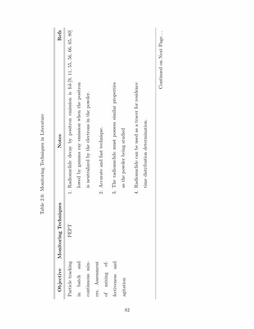
Tab
le2.
6:M
onit
orin
gT
echniq
ues
inL
iter
ature
Ob
ject
ive
Monit
ori
ng
Tech
niq
ues
Note
sR
efs
Par
ticl
etr
ackin
g
inbat
chan
d
conti
nuou
sm
ix-
ers.
Ass
essm
ent
ofm
ixin
gef
-
fect
iven
ess
and
agit
atio
n
PE
PT
1.R
adio
nucl
ide
dec
ayby
pos
itro
nem
issi
onis
fol-
low
edby
gam
ma
ray
emis
sion
when
the
pos
itro
n
isneu
tral
ized
by
the
elec
tron
sin
the
pow
der
.
2.A
ccura
tean
dfa
stte
chniq
ue.
3.T
he
radio
nucl
ide
must
pos
sess
sim
ilar
pro
per
ties
asth
ep
owder
bei
ng
studie
d
4.R
adio
nucl
ide
can
be
use
das
atr
acer
for
resi
den
ce
tim
edis
trib
uti
ondet
erm
inat
ion.
[9,
11,
55,
56,
66,
65,
80]
Con
tinued
onN
ext
Pag
e...
82

Ob
ject
ive
Monit
ori
ng
Tech
niq
ues
Note
sR
efs
Par
ticl
etr
ackin
g
inbat
chan
d
conti
nuou
sm
ix-
ers.
Ass
essm
ent
ofm
ixin
gef
-
fect
iven
ess
and
agit
atio
n
MR
I1.
Hydro
gen
nucl
eire
sonat
ew
ith
exte
rnal
mag
net
ic
fiel
dgi
vin
gth
ep
osit
ion
ofth
ehydro
gen
atom
s
2.P
owder
was
dop
edw
ith
anor
ganic
oil
that
isM
RI
sensi
tive
and
the
pow
der
mov
emen
tw
asfo
llow
ed
inth
em
ixer
3.Is
com
par
able
toth
e“f
reez
ing”
and
imag
ing
tech
-
niq
ue
and
isal
sofa
ster
[94]
Par
ticl
etr
ackin
g
inbat
chan
d
conti
nuou
sm
ix-
ers.
Ass
essm
ent
ofm
ixin
gef
-
fect
iven
ess
and
agit
atio
n
Rad
iopill
1.A
radio
freq
uen
cytr
ansm
itte
ris
inse
rted
into
the
pow
der
mas
san
dan
aeri
alnet
wor
kis
use
dto
de-
tect
the
pos
itio
nan
dve
loci
tyof
the
pill
2.U
sefu
lto
give
bulk
pow
der
mov
emen
tch
arac
ter-
isti
cslike
circ
ula
tion
velo
citi
es,
angu
lar
velo
citi
es
and
aver
age
velo
citi
es
3.Saf
eras
the
met
hod
does
not
invo
lve
radio
acti
ve
subst
ance
s
[17]
Con
tinued
onN
ext
Pag
e...
83

Ob
ject
ive
Monit
ori
ng
Tech
niq
ues
Note
sR
efs
Par
ticl
etr
ackin
g
inbat
chan
d
conti
nuou
sm
ix-
ers.
Ass
essm
ent
ofm
ixin
gef
-
fect
iven
ess
and
agit
atio
n
Ther
mis
tor
1.A
Ther
mis
tor
wit
hep
oxy
coat
ing
pro
tect
ing
the
core
was
use
d
2.T
he
Tri
bo-
elec
tric
senso
rw
asa
stai
nle
ssst
eel
pro
be
that
was
sensi
tive
inth
enA
curr
ent
leve
ls
3.T
he
curr
ent
and
the
resi
stan
cefr
omT
her
mis
tor
was
use
dto
calc
ula
teth
ehea
ttr
ansf
erco
effici
ent
bet
wee
nth
eT
her
mis
tor
and
the
pow
der
was
ex-
per
imen
tally
4.A
nag
itat
ion
index
was
defi
ned
bas
edon
diff
eren
ce
inth
ehea
ttr
ansf
erco
effici
ent
inst
atic
pow
der
and
the
agit
ated
pow
der
[90]
Con
tinued
onN
ext
Pag
e...
84

Ob
ject
ive
Monit
ori
ng
Tech
niq
ues
Note
sR
efs
Par
ticl
etr
ackin
g
inbat
chan
d
conti
nuou
sm
ix-
ers.
Ass
essm
ent
ofm
ixin
gef
-
fect
iven
ess
and
agit
atio
n
Cap
acit
orse
nso
r1.
Ach
arge
tran
sfer
typ
ese
nso
rw
asuse
2.V
oidag
ew
asm
easu
red
atdiff
eren
tp
osit
ions
ofth
e
bla
de
angl
eas
mix
ing
pro
ceed
ed
[86]
Sam
pling
and
Char
acte
riza
-
tion
ofm
ixin
g
pro
cess
NIR
1.A
NIR
spec
trop
hot
omet
eris
use
dw
ith
afib
erop
-
tic
pro
be
wit
hw
hic
hth
eco
nce
ntr
atio
ns
ofth
e
sam
ple
sar
eca
libra
ted
2.T
he
scan
tim
eis
ofth
eor
der
of15
seco
nds
toob
-
tain
stat
isti
cally
good
resu
lts.
3.A
ccura
tem
easu
rem
ents
ofsa
mple
conce
ntr
atio
ns
wer
ep
ossi
ble
[40,
48]
Con
tinued
onN
ext
Pag
e...
85

Ob
ject
ive
Monit
ori
ng
Tech
niq
ues
Note
sR
efs
Sam
pling
and
Char
acte
riza
-
tion
ofm
ixin
g
pro
cess
LIF
1.U
Vligh
tis
shin
edon
the
sam
ple
whic
hre
flec
ts
ligh
tat
low
erfr
equen
cies
whic
his
mea
sure
dan
d
calibra
ted.
2.T
he
met
hod
isfa
stco
mpar
edto
NIR
mea
sure
men
t
tech
niq
ues
3.N
otal
lp
owder
sfluor
esce
[52]
Sam
pling
and
Char
acte
riza
-
tion
ofm
ixin
g
pro
cess
FT
IR1.
Con
sist
sof
aF
ouri
erT
ransf
orm
Ram
anSp
ec-
trop
hot
omet
erw
ith
aF
ibre
opti
cpro
be
2.Sig
nal
was
wea
ker
than
that
inN
IRsp
ectr
osco
py
but
was
less
com
plica
ted
and
was
easi
lyuse
din
anal
ysi
s
[98]
Con
tinued
onN
ext
Pag
e...
86

Ob
ject
ive
Monit
ori
ng
Tech
niq
ues
Note
sR
efs
Sam
pling
and
Char
acte
riza
-
tion
ofm
ixin
g
pro
cess
Opti
cal
senso
r1.
Col
ordiff
eren
ceb
etw
een
the
com
pon
ents
use
dto
find
the
hom
ogen
eity
ofble
nd
2.F
iber
opti
cpro
bes
can
tran
smit
the
ligh
tw
ithou
t
any
noi
seco
rrupti
on
[47,
104,
103,
109]
End
ofT
able
87
2.5 Conclusion
Continuous dry powder blending offers many benefits. Employing parallel units avoids
scale up issues. Capital and space requirements are considerably reduced. As the
process is under steady state, process control using process analytical techniques is
easily implemented. Material containment is achieved reducing cross-contamination
of products and employee exposure. Also material in work-in-process being small in
quantity, there is considerable increase in flexibility and decrease in risk.
Industrially, batch blending systems were used to handle small volumes. Continu-
ous blending is a very good option for materials processed in large volumes. Continu-
ous powder blending needs accurate feeding systems. It also increases the complexity
in analysis by introducing flow in spatial dimension. Little emphasis was laid on
research in continuous powder blending compared to batch blending. But now, with
the advancement in electronics, online monitoring and control has become quick and
reliable. Feeding systems using electronic weigh feeders have also been shown to be
reliable. Therefore, continuous powder blending is an attractive alternative for large
volume processing in the pharmaceutical industry where traditionally batch blend-
ing is in place. However, investigations on the behavior of cohesive pharmaceutical
powders in these systems need to be pursued.
This paper reviews the developments in continuous blending since the last review
of Williams. The following conclusions can be made on state of the current research
on continuous blending:
1. A continuous blender can only reduce the short-term (high frequency) fluctu-
ations introduced by the feeding mechanism. Hence the design of the feeding
system takes a critical role in design of continuous blenders. The demand posed
on the blender performance can be greatly reduced by designing a feeding sys-
tem that is consistent and accurate.
2. The formation of slip planes (powder failure zone) in the powders due to the
movement of the blender mixing elements combined with the powder proper-
ties like the size, shape and topology determines the powder movement inside
88
the blender. This in turn determines the RTD of the powder in the blender.
Therefore, the mean failure zone height and spacing are important characteristic
length scales in blender design
3. Techniques like PEPT and MRI offer the advantage of visualizing the dynamics
in 3D while blending is in progress. The effect of powder properties and blender
operational parameters on powder movement and blending performance can be
studied in real time using these techniques giving useful insights on the efficacy
of the blender. These techniques offer the additional advantage of determining
parameters like dispersion coefficient from average particle movement inside the
blender. These parameters can then be used in predicting the RTD and hence
the size of the blender for a given load and VRR requirement
4. Cohesive powders are very common in many industries like pharmaceuticals.
These powders, which fall in the size range 0.5 - 200 µm, need to be investi-
gated in continuous blenders. Consistent feeding of powders that do not flow
freely is a considerable challenge in feeding system design. Studies on cohesive
powders should concentrate on designing an efficient feeding system that deliv-
ers the consistency demanded by the continuous blender. Also, the mechanisms
of mixing for cohesive powders in such continuous blenders are not clear. Ef-
forts must be directed towards investigating the movement of these powders in
continuous blenders
In a review on continuous mixing of solids, Williams [105] commented that predic-
tion of blender performance from a fundamental particle movement study in continu-
ous blenders were valuable but not practical. As process understanding is important
to minimize the risk of operations in the pharmaceutical industry, understanding
particle interactions and translating these microscopic interactions into macroscopic
powder behavior is necessary.
Though mathematical modeling and prediction of the blender performance may be
very difficult, the current available technology can be used effectively in performing
a multi-scale analysis of the behavior of powders in continuous blenders. Further
89

research is needed in establishing a connection between the particle characteristics,
blender operational parameters and the particle movement under the influence of the
blender mixing elements with the performance of the continuous blender.
90
Chapter 3
Thesis Objectives
The main goal of this thesis was to test and understand a continuous blending sys-
tem for mixing dry pharmaceutical powders. A satisfactory understanding of the
continuous blending process should uncover the underlying relationships between the
properties of raw materials, the qualtiy attributes of the product of the process and
the operating conditions.
Ngai [71] used a multi-scale analysis framework to establish the relationships be-
tween fundamental particle parameters like size, cohesion/adhesion surface energies
and friction with macroscopically observed phenomena occuring during batch mix-
ing. In this work, we utilised a similar framework to understand the dependence
of the performance of continuous dry powder blending system with blender design
parameters, operating variables and material properties. However, as noted later the
main approach in this work is experimental in nature whereby various particle and
operational parameters are varied experimentally and the experimental blending per-
formance determined. The work was pursued in two parts catering to two different
objectives as outlined below. A third objective based on the management education
of the program focused on creating and applying a framework for internationalization
of pharmaceutical and biologics manufacturing.
3.1 Specific Objectives
In order to achieve the aforementioned goal of developing a phenomenological un-
derstanding of dry powder continuous blending and its impact in pharmaceutical
91

manufacturing, the following objectives are proposed.
3.1.1 Investigation of powder flow behavior
The flow behavior of powders in different blender geometries was to be studied using
stimulus-response techniques. These studies were to focus on understanding the effect
of particle-particle interactions alongwith the influence of material properties on the
performance of dry powder blending blending. Residence time distributions of the
continuous blenders was to be modeled using simple models like Dispersion model.
It was expected that the parameters in such models (for e.g., axial dispersion co-
efficient) could be a function of the macroscopic and microscopic properties of the
powders and the conditions under which the experiments were conducted. It was
proposed to study this underlying dependence of dispersion coefficient on fundamen-
tal particle properties like cohesion and adhesion surface energies, particle sizes and
operational variables like rotation rates and flow rates of the material in the blender.
3.1.2 Understanding macroscopic blending behavior
The macroscopic behavior of continuous dry powder blending system will be studied.
The influence of design parameters and operating variables on process performance
will be assessed. The phenomenological, microscopic understanding from the last
phase will be integrated with the operational, macroscopic understanding of the cur-
rent phase to tease out key design principles in continuous dry powder blending.
A relationship for theoretically estimating the VRR was described in equation (2.3).
This was to be utilised in predicting the performance of the continuous blending sys-
tem and compared with the experimental VRR. A valid prediction of the continuous
blenders performance was expected to be a critical tool in both design and control of
the continuous blending process.
3.1.3 Analyzing economics of continuous blending
The economic analysis of implementing dry powder continuous blending in the phar-
maceutical industry will need focus on integrating and translating the potential de-
92

crease in capital investment and production cycle times into financial benefits. This
analysis should serve to justify the value addition in implementing continuous powder
blending.
The current manufacturing paradigm in the pharmaceutical industry is one of
quality-by-inspection. Under this paradigm, the product is rigorously tested for quality
at several stages of the manufacturing process. This adds considerable delay in the
production cycle causing increased work-in-progress inventories. The FDA recently
recommended moving to a new paradigm, one of quality-by-design. Under this new
paradigm, quality of the product would have to be built in the design phase and
the product would need very minimal quality assurance steps in the manufacturing
process. Continuous manufacturing in general and continous blending in particular
are processes that are amenable to the quality-by-design paradigm. The economic
argument for implementing continuous blending will not be investigated in this thesis.
3.1.4 Framework for Globalization of Manufacturing
While technology and processed based competitive advantage of pharmaceutical com-
panies was the primary focus of this thesis, the capstone project aimed to identify a
framework for globalization of pharmaceutical and biologics manufacturing that could
be useful for operations managers in making the right location choices.
93

94

Chapter 4
Method of Approach
Domike [25] and Ngai [71] have shown the importance of particle adhesion and cohe-
sion on the macroscopic behavior of powders in processes like blending and phenom-
ena like flow of powders in piles and heaps. This multiscale analysis framework can
be utilised in understanding the behavior and pharmaceutical powders in continuous
blending systems. In order to experimentally understand the effect of operational
variables and particle parameters, two different blenders and six different powders
(API and Excipients) were investigated over a range of operational variables.
4.1 Choice of Continuous Blender
Literature on continuous mixing argued that mixers imparting high shear and flu-
idization energy while mixing the powders caused problems with segregation. On the
other hand mixers imparting low shear by convection avoid segregation problems but
mix the powders only to a certain degree of performance. In this work a high shear
fludizing mixer and moderate shear mixer were examined. A Patterson Kelley & Co.
ZigzagR© blender and a ribbon blender designed in-house were chosen as the choices
for the blending system.
4.1.1 Patterson Kelley ZigZag Blender
A plant scale ZigzagR© blender (at Patterson-Kelley & Co., East Stroudsburg, PA.),
shown in figure 4-1, consists of a drum section that houses an intensifier bar and a
V section which drives the powder from the inlet to the outlet. The design of the
95
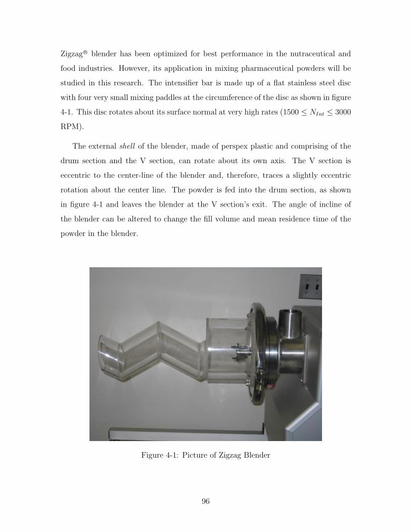
ZigzagR© blender has been optimized for best performance in the nutraceutical and
food industries. However, its application in mixing pharmaceutical powders will be
studied in this research. The intensifier bar is made up of a flat stainless steel disc
with four very small mixing paddles at the circumference of the disc as shown in figure
4-1. This disc rotates about its surface normal at very high rates (1500 ≤ NInt ≤ 3000
RPM).
The external shell of the blender, made of perspex plastic and comprising of the
drum section and the V section, can rotate about its own axis. The V section is
eccentric to the center-line of the blender and, therefore, traces a slightly eccentric
rotation about the center line. The powder is fed into the drum section, as shown
in figure 4-1 and leaves the blender at the V section’s exit. The angle of incline of
the blender can be altered to change the fill volume and mean residence time of the
powder in the blender.
Figure 4-1: Picture of Zigzag Blender
96
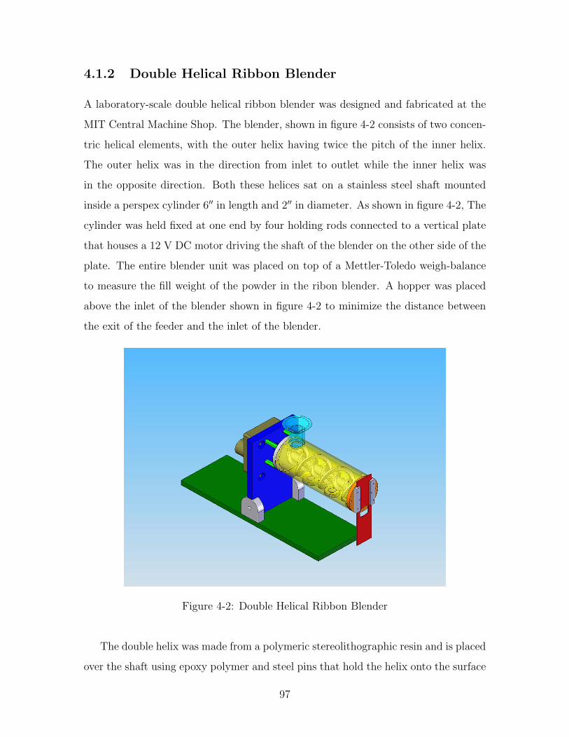
4.1.2 Double Helical Ribbon Blender
A laboratory-scale double helical ribbon blender was designed and fabricated at the
MIT Central Machine Shop. The blender, shown in figure 4-2 consists of two concen-
tric helical elements, with the outer helix having twice the pitch of the inner helix.
The outer helix was in the direction from inlet to outlet while the inner helix was
in the opposite direction. Both these helices sat on a stainless steel shaft mounted
inside a perspex cylinder 6′′ in length and 2′′ in diameter. As shown in figure 4-2, The
cylinder was held fixed at one end by four holding rods connected to a vertical plate
that houses a 12 V DC motor driving the shaft of the blender on the other side of the
plate. The entire blender unit was placed on top of a Mettler-Toledo weigh-balance
to measure the fill weight of the powder in the ribon blender. A hopper was placed
above the inlet of the blender shown in figure 4-2 to minimize the distance between
the exit of the feeder and the inlet of the blender.
Figure 4-2: Double Helical Ribbon Blender
The double helix was made from a polymeric stereolithographic resin and is placed
over the shaft using epoxy polymer and steel pins that hold the helix onto the surface
97

of the shaft. The length of the blender was chosen to be 6′′ and the diameter to be
2′′ by computing the hold-up volume required for an average mean residence time of
30s at 50% fill volume of lactose with a bulk density of 610 kg/m3 at a nominal flow
rate of 5 kg/hr. The pitch of the inner helix was set to twice that of the outer helix
with the expectation that, for every single rotation of the shaft, the powder in the
inner zone would“mix” with 2× the powder in the outer zone giving rise to increased
back-mixing. The process of fabricating the helical ribbon constrained increasing the
inner pitch any more than twice that of the outer pitch. A clearance of 0.5 mm was
kept between the wall of the blender and the outer helical ribbon. A radial clearance
of 5 mm was maintained between the two concentric inner and the outer helix in
order to have a buffer zone of powder mass where free surface is created due to the
opposing movements of the two helices.
The angle of incline of the blender could be set anywhere between −45◦ to +45◦
about the plate that holds the blender and the motor in place. Three quartz glass
windows are provided at the bottom side of the cylindrical perpex shell, in order to
measure the concentration of components using various analytical techniques. The
blender’s exit end cap has two open slots through which powder would flow out when
the blender is in action. A gate to close either of the exits was present, although,
it was never used and the blender was always run with the exit under fully open
conditions.
4.2 Powder Feeders
Feeding (dispensing) system plays a very critical role in determining the performance
of the overall blending system. An imprecise feeder can cause a blender to under-
perform, simply because the blender is unable to reduce the variance introduced by
the feeder in the inlet stream. Literature suggested that loss-in-weight (LIW) feeders
deliver material at very high precision and accuracy at all flow rates. Hence, LIW
feeders from Schenck Accurate Inc., Whitewater, WI, were used to feed the excipients
and APIs in this work. Schenck Accurate MechatronR© feeders were used to feed pow-
ders to the Patterson Kelley ZigzagR© blenders and Tuf-flexR© feeder was used to feed
98

the double helical ribbon blender. These feeders consist of counterbalanced hoppers
from which helix draws the powder out. An internal control system (Intecont PlusR©)
controls the feeding rate with a PID control algorithm, utilising the weight of the
counterbalanced hopper as the response from the system.
The MechatronR© feeders delivered three different flow rates ranges: 40 to 60 kg/hr,
0.5 to 5 kg/hr and 0.05 to 1 kg/hr. Different materials were fed at different rates,
depending on the concentrations of the ingredients, to the ZigzagR© blender. The
Tuf-flexR© feeder was rated between 1 and 10 kg/hr and was used to feed only the
excipient.
4.3 Sampling and Analytical Techniques
Two non-destructive analytical techniques were used in this work. Light Induced
Fluorescence works on the principle of excitation and relaxation of electrons from
and to ground state molecular orbitals. Near Infra-red Spectroscopy works on the
principle of vibrational excitation and relaxation of molecules.
4.3.1 Light Induced Fluorescence, LIF
When high energy radiation (like the photons in UV wavelength range of the electro-
magnetic spectrum) impinge on molecules with high resonance energies (like aromatic-
ring containing caffeine and acetaminophen) electrons are excited to higher energy
levels [52]. Relaxation of these electrons to lower energy levels occurs by emission
of a low wavelenghth radiation, a process called called fluorescence. At low enough
concentrations of the fluorescing molecule, the intensity of the emitted radiation is
proportional to the concentration of the fluorescing ingredient. Thus, this signal can
be used as a proxy for concentration of that ingredient in a mixture, especially a
powder mixture. However, this linearity in fluorescent signal to the the concentration
is lost at higher concentrations.
An LIF sensor, developed by Lai et al. [52] and manufactured by Honeywell Au-
tomation, (Honeywell, Morristown, NJ), was used to measure the concentration of
the active ingredient and has been described in detail elsewhere [52]. Caffeine was
99

Figure 4-3: Logarithmic LIF Calibration Curve
measured using XF-01 filter sets procured from Omega Filters (Omega Filters, Brat-
tleboro, VT). A fiber optic probe extension was used to reach the quartz glass near
the exit under the blender. The LIF signal was calibrated to the concentration of caf-
feine by shining LIF through a quartz glass window on premixed caffeine and lactose
of different concentrations.
Figure 4-4: Exponential LIF Calibration Curve
The calibration curve was found to be very non-linear and is shown in figures 4-3,
4-4 and 4-5. Two kinds of calibrations were pursued. In the first type, the signal was
100

directly calibrated to the concentration of caffeine, while in the second type the signal
was ratioed with background signal at 100% lactose concentration and this ratio was
calibrated with the concentration of caffeine. Figures 4-3, 4-4 and 4-5 show these
calibration curves. The calibration equations, parameters and R2 values are given in
table 4.1.
Figure 4-5: LIF Signal Ratio Calibration Curve
Table 4.1: LIF Calibration Parameters
# Equation Parameters R2
1 C = αSigβ α = 3× 10⁻¹⁹ β = 11.58 0.9701
2 C = α exp (β · Sig) α = 1.6× 10⁻⁴ β = 0.33 0.9992
3 C = α exp(β SigSig0
)α = 1.6× 10⁻⁶ β = 8.49 0.9992
4.3.2 Near Infra-red (NIR) Spectroscopy
The Equipartition Theorem states that the thermal energy of a substance is parti-
tioned equally into translational, vibrational and rotational energy states. Collisions
between molecules lead to exchanges in translational energies. When light falls on a
substance, some of it is absorbed by the molecules in the substance thereby exciting
some of the molecules into higher vibrational energy states. These molecules then
101
relax from the higher vibrational states by emitting electromagnetic radiation in the
Near Infrared (NIR) range. At low concentrations it has been shown by Kubelka and
Munk that the absorbance, log 1R
, is proportional to the concentration as described
by Olinger et al. [78]. R is the reflectance of the light falling on the sample and
absorbance is related to the concentration of a component in the mixture. Since
every compound has distinct vibrational energy states determined by the chemical
structure of the molecule, the NIR spectrum of a mixture carries information on all
the components in the mixture.
However, the observed spectra consist of a number of overlapping bands arising
from overtones and anharmonicities of the vibrational states. Therefore, the ab-
sorbance over the entire near-infra red range 1100−2500 cm-1 is measured to capture
the spectra of all the components. A calibration curve can be generated relating
the NIR spectra to the concentrations. However, as mentioned, the overtones and
anharmonicities of the spectra cause considerable analytical errors when multiple lin-
ear regression (MLR) is used[108]. Therefore, a partial least squares regression of
projections to latent structures (PLS) model is used to calibrate the NIR spectra to
concentrations [7, 8, 64].
An Axsun NIR Spectrometer (from Axsun Technologies, Billerica, MA) was em-
ployed in the experimental work. The spectrometer consists of a laser light source
inside a main block connected to an IntegraSpec R© integrating sphere via a fiber op-
tic cable. This integrating sphere collects the reflected light and transmits the light
through fiber optic cables to the photomultipliers in the main block. The collected
intensity is converted to absorbance after ratioing with the background taken using a
Spectralon sample (which has a reflectivity of 1.) The collected spectra are processed
using multivariate statistics software called SIMCA-P+ (Umetrics Inc., Kinnelon,
NJ). Data processing and subsequent analysis is described below.
Partial Least Squares by Projection to Latent Structures (PLS) is used to cali-
brate the NIR sensor. The experimental technique involved pre-blending mixtures
of different APIs and different excipients in a V-blender for half an hour and then
taking 25 NIR spectra by dividing the powder from the V-blender into two samples of
102

Figure 4-6: PLS Calibration Plot for Caffeine and Lactose DCL14 Mixture
approximately equal weight at the same location as the collection during the blending
process. Each of these spectra are first converted scaled to a unit variance, then a first
derivative 11 point Savitzky-Golay transform is applied. Following this, a standard
normal variate transform is applied. These transformed spectra are devoid of errors
arising from changes in density, particle size and external light.
PLS regression on this data model that had R2 values between 0.95 and 0.98.
Figure 4-6 shows an example PLS calibration plots where the predicted and actual
concentrations of the mixture are plotted on X and Y axis. The number of terms, R2
values and Q2 which is a measure statistically accuracy of the predictions is given in
table 4.2
Table 4.2: PLS Calibration of NIR Spectra
# API Excipient Ncomp R2 Q2
1 Caffeine DCL 11 3 0.991 0.991
2 Caffeine DCL 14 4 0.987 0.987
3 Caffeine MCC 2 0.973 0.973
103

# API Excipient Ncomp R2 Q2
4 Acetaminophen DCL 11 1 0.99 0.99
5 Acetaminophen DCL 14 3 0.987 0.987
6 Acetaminophen MCC 2 0.983 0.983
Three component calibration was performed by blending varying concentrations of
Magnesium Stearate, Caffeine and Lactose DCL-11 in a V-blender for half hour. The
mixture was divided into two samples by collecting the powder in the two different
legs of the V blender into two differnt weighing dishes. The powder samples from the
blender were placed on the quartz glass window of the ribbon blender and 25 NIR
spectra were taken for each sample. The concentration of MgSt was varied between
0.01, 0.02, 0.03, 0.25, 0.5 and 0.75 and caffeine was varied between 0.05, 0.1, 0.2, 0.3
and 0.25, 0.5 and 0.75. The PLS calibration of the multicomponent NIR spectra after
pre-processing gave a PLS model with an R2 value of 0.90 for Caffeine and 0.93 for
MgSt as shown in figures 4-7 and 4-8
Figure 4-7: PLS Calibration for Caffeine in (Caffeine+Lactose+MgSt) Three Com-ponent System
It was hypothesized that the pre-blended powder mixture had not achieved steady
state in the batch V-blender due to the presence of MgSt due to inadequate blending
time. This was expected to have caused the calibration model to yield an unsatis-
104
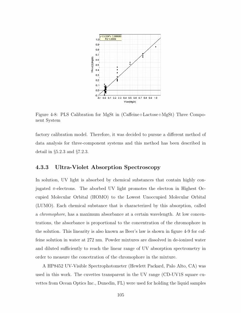
Figure 4-8: PLS Calibration for MgSt in (Caffeine+Lactose+MgSt) Three Compo-nent System
factory calibration model. Therefore, it was decided to pursue a different method of
data analysis for three-component systems and this method has been described in
detail in §5.2.3 and §7.2.3.
4.3.3 Ultra-Violet Absorption Spectroscopy
In solution, UV light is absorbed by chemical substances that contain highly con-
jugated π-electrons. The aborbed UV light promotes the electron in Highest Oc-
cupied Molecular Orbital (HOMO) to the Lowest Unoccupied Molecular Orbital
(LUMO). Each chemical substance that is characterized by this absorption, called
a chromophore, has a maximum absorbance at a certain wavelength. At low concen-
trations, the absorbance is proportional to the concentration of the chromophore in
the solution. This linearity is also known as Beer’s law is shown in figure 4-9 for caf-
feine solution in water at 272 nm. Powder mixtures are dissolved in de-ionized water
and diluted sufficiently to reach the linear range of UV absorption spectrometry in
order to measure the concetration of the chromophore in the mixture.
A HP8452 UV-Visible Spectrophotometer (Hewlett Packard, Palo Alto, CA) was
used in this work. The cuvettes transparent in the UV range (CD-UV1S square cu-
vettes from Ocean Optics Inc., Dunedin, FL) were used for holding the liquid samples
105
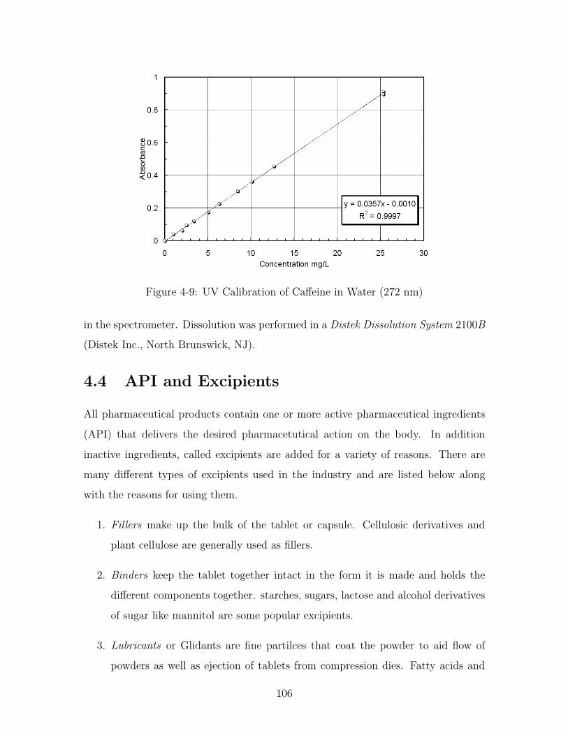
Figure 4-9: UV Calibration of Caffeine in Water (272 nm)
in the spectrometer. Dissolution was performed in a Distek Dissolution System 2100B
(Distek Inc., North Brunswick, NJ).
4.4 API and Excipients
All pharmaceutical products contain one or more active pharmaceutical ingredients
(API) that delivers the desired pharmacetutical action on the body. In addition
inactive ingredients, called excipients are added for a variety of reasons. There are
many different types of excipients used in the industry and are listed below along
with the reasons for using them.
1. Fillers make up the bulk of the tablet or capsule. Cellulosic derivatives and
plant cellulose are generally used as fillers.
2. Binders keep the tablet together intact in the form it is made and holds the
different components together. starches, sugars, lactose and alcohol derivatives
of sugar like mannitol are some popular excipients.
3. Lubricants or Glidants are fine partilces that coat the powder to aid flow of
powders as well as ejection of tablets from compression dies. Fatty acids and
106
their salts like magnesium stearate and silica are a few popular lubricants.
4. Coatings prevent attack of tablets by moisture and aid in consumption of tablets
by changing their taste. Coatings are usually cellulose derivatives and some-
times made up of proteins from corn
5. Flavors, Colors and Sweeteners are added in small quantities to enhance the
look, feel and taste of the tablet or capsule and usually do not serve any other
purpose.
Domike [25] and Ngai [71] have studied the interparticle forces of adhesion for caf-
feine and popularly used excipients in the pharmaceutical industry, micro-crystalline
cellulose and lactose. As one of the goals of the project is to understand the effect
of microscopic properties of powders on the macroscopic phenomena in continuous
blending, the choice of API and excipients was made based on the availability of
experimentally determined microscopic properties like cohesion, adhesion surface en-
ergies and friction coefficients of powders. Table 4.3 shows the various properties of
relevance of individual powders used in this work. The mean and standard deviations
of the cohesion energies per unit area are shown under µ and σ respectively.
4.4.1 Caffeine
Anhydrous Caffeine (1,3,7-trimethyl Xanthine) is a xanthine alkaloid and a central
nervous system stimulant. USP grade caffeine powder was obtained from Sigma
Aldrich (Sigma Inc., St. Louis, MO.) Caffeine is a white powder that has a melting
point of 238◦C. ESEM pictures of caffeine particles are shown in [71]. Caffeine is
an irregularly shaped particle that has particle size of 196 µm with a very large
standard deviation of about 100 µm. Caffeine is not a free flowing powder and
usually agglomerates in the presence of atmospheric moisture. Therefore, caffeine
was manually de-agglomerated before all experiments. The density of caffeine varied
between 0.41 g/cc and 0.53 g/cc depending on whether the caffeine powder was outside
exposed to the atmosphere for a long time (overnight) or was freshly removed from
an air-tight container. The mass-volume curve is shown in figure 4-10.
107

Figure 4-10: Mass Volume Curve for Caffeine Stored Outside and Inside an AirtightContainer
108
4.4.2 Acetaminophen
Acetaminophen (N-(4-hydroxyphenyl)-Acetamide) is widely used as an analgesic and
anti-pyretic and is the active ingredient in the popular OTC drug Tylenol R©. Ac-
etaminophen was obtained from Sigma Aldrich (Sigma Inc, St. Louis, MO) and is a
white powder with a melting point of 169◦C. Acetaminophen has a bulk density of
1.293g/cc. Acetaminophen agglomerates in the presence of moisture and anhydrous
acetaminophen was used in all the experiments. Acetaminophen, too, was de-clumped
as and when required.
4.4.3 Lactose
Lactose (a disaccharide that consists of β-D-galactose and β-D-glucose molecules
bonded through a β1-4 glycosidic linkage, 4-o-β-D-pyranosyl D-Glucose) is a white
powder that is found in both amorphous and crystalline forms depending on the
process of synthesis. Spray dried lactose usually gives spherical particles, that has
superior flow characteristics and at the same time is cohesive enough to act as a binder
in the tablet. Two grades of direct compressible lactose (DCL) have been used in this
work. Both these grades were procured from DMV-International (DMV-Fonterra
Excipients, Delhi, NY). The bulk density of both the grades of lactose was 0.61g/cc.
Lactose is less cohesive than microcrystalline cellulose with a mean cohesion surface
energy of 0.52 and a standard deviation of 0.41 mJ/m2.
1. Direct Compressible Lactose (DCL) - 11 has a mean particle size of 100µm with
a standard deviation of 50µm with a log-normal distribution. DCL-11 is spray
dried lactose and contains a mixture of α-lactose monohydrate crystals with
some amorphous lactose. DCL-11 consists of spherical particles that has very
good flow characteristics. However, DCL-11 possesses the tendency of caking
in the presence of moisture and gravity. This mild caking tendency was not a
problem in delivering the material through the Schenck Accurate R© feeder since
the design of the feeder takes this caking into account and the hopper walls in
the feeder massaged the powder thereby breaking the agglomerates. An SEM
109

image of DCL-11 is shown in [24].
2. Direct Compressible Lactose (DCL) - 14 has a mean particle size of 110µm
with a standard deviation of 70µm with a log-normal distribution. DCL-14 is
also a spray-dried grade of lactose consisting of a mixture of α-lactose monohy-
drate crystals mixed with greater proportions of amorphous lactose. While the
characteristics of this grade of lactose is similar to that of DCL-11, the particle
sizes distribution is considerable wider. DCL-14 posed a reduced risk of caking
in the feeder due to the presence of a wider distribution of particles reducing
the possibility of increased stresses in the material. For some of the experi-
ments, DCL 14 was sieved into powders of two different particle size ranges
40 ≤ D50 ≤ 150µm and 150 ≤ D50 ≤ 250µm. Both these powders were
evaluated for the effect of particle size on blending. An SEM image of DCL-11
is shown in [24].
3. HMS Impalpable Lactose has a mean particle size of 90µm. HMS Impalpable
lactose is α-lactose monohydrate in amorphous form. It is non-spherical and
has a higher surface area compared to other grades of lactose. HMS lactose
flows very irregularly and agglomerates very easily. These powders were tested
in both types of blenders in this work. The powder due to its inability to
flow easilty clogged the ribbon blender, but performed very well in the Zigzag R©
blender. The powder required considerable amount of shear forces to mobilize
and the the Zigzag R© blender supplied the required energy to move and blend
this excipient.
4.4.4 Microcrystalline cellulose
Cellulose is a biopolymer present widely present in plants and plant extracts. Cellulose
is a long chain polymeric polysaccharide carbohydrate of β-D-Glucose, is generally
used as a filler in tablets. Microcrystalline Cellulose facilitates quicker disintegration
of tablets exposing the API to the liquids in the body in addition to acting as a
undigested dietary fiber. Two grades of cellulose were used in this work. MCC
110

comparatively more cohesive than lactose. The cohesive surface energy of MCC has
a mean of 1.58 and standard deviation of 0.96 mJ/m2.
1. Avicel R© microcrystalline cellulose PH-102 has a mean particle size of 100µm is
an irregular sized particle with a flat flaky microscopic structure as shown in the
ESEM picture figure 4-11. Avicel R© was procured from FMC Biopolymer(FMC
Biopolymer, Philadelphia, PA) and has bulk density of 0.3 g/cc. Avicel R© flow
behavior is very erratic and is highly influenced by moisture. In the absence of
moisture, electrostatic forces on Avicel R© particles cause it to flow erratically.
Avicel R© usually has a moisture content of 3 − 5% by weight.
Figure 4-11: ESEM of Avicel MCC PH102
2. Celphere R© microcrystalline cellulose CP-102 has a mean particle size of 150µm
is an spherical particle as described in [31]. Celphere R© was procured from Asahi
Kasei (Asahi Corp.,Tokyo, Japan) and has bulk density of 0.83 g/cc. Celphere R©
flow behavior is less erratic than Avicel. However, Celphere R© is less frequently
used in the pharmaceutical formulations than Avicel R©/
4.4.5 Magnesium Stearate, MgSt
Magnesium Stearate (MgSt) is a white amorphous powder comprising of fine particles
in the size range 20 to 70 µm. It is a generally recognized as safe (GRAS) substance
and is sourced from vegetable oil or animal fat. The MgSt used in all our experiments
111

were vegetable sourced and were procured from Sigma Aldrich (Sigma, St. Louis,
MO). MgSt is used as a lubricant in the pharmaceutical industry and aids in the
flowability of powders. It also aids in the ejection of the table from the tablet die and
acts by coating the surface of the die with fine particles of MgSt which reduce the
cohesive forces between the tablet and the die wall [101].
112
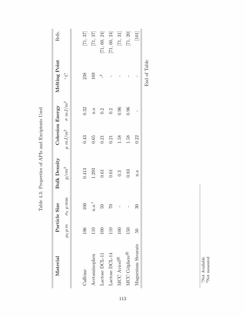
Tab
le4.
3:P
rop
erti
esof
AP
Isan
dE
xci
pie
nts
Use
d
Mate
rial
Part
icle
Siz
eB
ulk
Densi
tyC
ohesi
on
Energ
yM
elt
ing
Poin
tR
efs.
µVµm
σVµm
mg/cm
3µmJ/m
2σmJ/m
2◦C
Caff
eine
196
100
0.41
30.
430.
3223
8[7
1,37
]
Ace
tam
inop
hen
110
n.a
.11.
293
0.65
n.a
169
[71,
37]
Lac
tose
DC
L-1
110
050
0.61
0.21
0.2
-2[7
1,60
,24
]
Lac
tose
DC
L-1
411
070
0.61
0.21
0.2
-[7
1,60
,24
]
MC
CA
vic
elR ©
100
-0.
31.
580.
96-
[71,
31]
MC
CC
elpher
eR ©
150
-0.
831.
580.
96-
[71,
20]
Mag
nes
ium
Ste
arat
e50
30n.a
0.22
--
[101
]
End
ofT
able
1N
otA
vaila
ble
2N
otm
easu
red
113

4.5 Flow Behavior Experiments
Simple impulse response experiments with an impulse input of the active ingredient
in a continuous blender where the excipient is constantly flowing through the system
can be used to compute the residence time distribution of the active in the blender.
This residence time distribution can then be abstracted to a fewer set of parameters
like the Axial Dispersion Coefficient (or simply Dispersion Coefficient, D) and the
velocity (or space time if length of the blender is fixed, also called the Transport
Coefficient, T ) which is useful in comparing and understanding the mobility of the
active ingredient in the blender.
4.5.1 Axial Dispersion Model
In axially mixed systems, such as a double helical ribbon blender and rotating drum
blender, the residence time distribution can be modeled using an axial dispersion
model [81, 104, 103, 48]. In moderate to high shear mixing systems like the NautamixR©
and the ZigzagR© blenders, the residence time distribution normally follows a ideal
blender followed by plug flow blender model [47].
Axial dispersion model given by equation 2.8 describe the movement of powders in
axially mixed systems. Following Fogler [32] non-dimensionalized this Fokker Planck
Equation using, θ = tVL
, ζ = xL
, Ψ = CM/V
and Bo = V LD , where Bo is the Bodenstein
number (Peclet number for liquids), L is the length of the mixer and V is the average
(mean) velocity of the powder in the mixer, we get equation (4.1).
∂Ψ
∂ θ= −∂Ψ
∂ ζ+
1
Bo
∂2 Ψ
∂ ζ2(4.1)
The initial condition for solving this equation is given by.
Ψ(0+, 0
)= 0 (4.2)
We can solve this PDE given the boundary conditions for an impulse input. There
are three different kinds of boundary conditions called the Danckwerts’ Boundary
114

Conditions.
4.5.1.1 Closed-Closed Boundary Condition
When dispersion does not occur both upstream and downstream of the mixing sec-
tion in a blender (i.e. points upstream to tracer addition and downstream to tracer
measurement), the boundary conditions are called closed-closed boundary conditions.
Mathematically this is represented by,
[− 1
Bo
∂Ψ
∂ ζ
]0
+ [Ψ]0 = 1 (4.3)[∂Ψ
∂ ζ
]1
= 0 (4.4)
Using the closed-closed boundary conditions in equations (4.3) and (4.4), and the
initial condition from equation (4.2), the dispersion equation (4.1) can only be solved
numerically.
4.5.1.2 Open-Open Boundary Condition
Dispersion occurs both upstream and downstream of the mixing section in a blender
(i.e. points upstream to tracer addition and downstream to tracer measurement), the
boundary conditions are called closed-closed boundary conditions. Mathematically
this is represented by,
[∂Ψ
∂ ζ
]0+
=
[∂Ψ
∂ ζ
]0−
(4.5)
[Ψ]0+ = [Ψ]0− (4.6)[∂Ψ
∂ ζ
]1+
=
[∂Ψ
∂ ζ
]1−
(4.7)
[Ψ]1+ = [Ψ]1− (4.8)
Using the closed-closed boundary conditions in equations (4.5) to (4.8), and the
initial condition from equation (4.2), the dispersion equation (4.1) be solved un-
der certain conditions to give the concentration at the exit of the blender E (t) =
115
Ψ(ζ = 1, θ = t
τ
).
E (t) =1
2 τ√(
πBo
) (tτ
)3 exp
(−(1−
(tτ
))2(4 tτBo
) )(4.9)
This model is true only if the length of the blender is considerably larger than the
characteristic length of dispersion. In many of the real blending cases, this condition
is satisfied. The most important parameter in this model is the Bodenstein number
and can be estimated by performing non-linear regression of the observed response
to a unit impulse in the continuous blender.
4.5.2 Determination of Residence Time Distribution
The response from Impulse response experiments are usually concentration curves as
a function of time, beginning with time t = 0 when the tracer (API in the case of
determining RTD of blending of powders) is introduced. The concentration curves
can be converted to residence time distribution and the mean residence time by two
different methods. In the first method, both the RTD and mean residence time can
be computed using the equations (4.10) and (4.11).
E(ti) =C(ti)∑
iC(ti)(ti − ti−1)(4.10)
〈t〉 =∑i
tiE(ti)(ti − ti−1) (4.11)
Alternatively, we can estimate the space time τ of the tracer (API) and the Boden-
stein number Bo in the blender by using equation (4.9), but by taking into account
a multiplying factor A that converts concentration curves into residence time distri-
bution. We note that parameter A is a measure of the area under the concentration
curve given by the denominator in the equation (4.10). Therefore, we can use the
concentration curves to estimate A, τ and Bodenstein number (or D) at the same
time as shown in equation (4.12)
116

C (t) =A
2 τ√(
πBo
) (tτ
)3 exp
(−(1−
(tτ
))2(4 tτBo
) )(4.12)
4.5.3 Summary
The approach, therefore, consisted of measuring the impusle response of the con-
tinuous blending system, modeling the residence time distribution with simple RTD
models, like Axial Dispersion models, and subsequently predicting the variance re-
duction ratios for sinusoidal and other kinds of inputs to the blender. Experiments
will be performed with different combinations of excipients and APIs in order to un-
derstand the effect the cohesive and adhesive forces on the behavior of powders in
continuous blenders.
4.6 Blending Experiments
Two component and three component blending experiments can be carried out to
assess the performance of a continuous blending system. Literature suggested that a
continuous blender mixing non-segregating, non-cohesive powders can reduce variance
introduced by disturbances of time periods less than the mean residence time of the
continuous blender. A model for the blender would relate the performance of the
blender to the flow behavior in the blender and the input characteristics at the feeder.
4.6.1 Theoretical Variance Reduction Ratio
The variance reduction ratio of a continuous dry powder blender with a residence
time distribution E(t) and a feeding input with autocorrelation R(t′) is given by
equation (2.3). The output of a continuous blending system depends on the forc-
ing function (feeding input) and the system response of the blender to that forcing
function. In other words, one other way to arrive at equation (2.3), is by taking
the convolution integral of the input forcing function, Cin (t) and RTD, E (t) and
subsequently taking the variance ratio at steady state of the output.
117

Cout (t) = E (t) ⊗ Cin (t) (4.13)
⇒ Cout (t) =
t∫0
E (t′) Cin (t− t′) dt′ (4.14)
=
t∫0
E (t− t′) Cin (t′) dt′ (4.15)
V RR =var (Cout,ss (t))
var (Cin (t))(4.16)
When the blender is an ideal blender, the residence time distribution follows and
exponential decay as discussed by Danckwerts [21] and given by equation (4.17). For
a sinusoidal forcing function, given by equation (4.18), we can compute the auto-
correlation from equation (2.2) to give:
Eideal (t) =1
τexp
(− tτ
)(4.17)
Cin (t) = b sin
(2π
t
td
)(4.18)
Rin (t′) =
limT→∞
1T
T∫0
Cin (t)Cin (t+ t′) d t
σ2(4.19)
⇒ Rin (t′) = cos
(2πt′
td
)(4.20)
Then, we can use either equation (4.15) with (4.16) or equation (4.20) with (2.3)
and compute the VRR to be:
V RRsin = 1 +
(τ
td
)2
(4.21)
where τ = WF
is the space time of the blender, W is the fill weight of the blender,
F is the flow rate of the powder in the blender, td is the time period of the forcing func-
tion (disturbance) entering the blender. As we see from equation (4.21), the Variance
reduction ratio is proportional to the residence time and inversely proportional to
the time period disturbance. Equation (4.21) suggests that an ideal blender behaves
as a first order low pass filter, allowing disturbances with time periods greater than
118

space time (τ , which in this case is the mean residence time too) to pass through the
blender. All disturbances whose time-periods are lesser than τ , the blender reduces
the fluctuations at those frequencies as shown in figure 4-12.
Figure 4-12: Effect of Input Fluctuation
4.6.2 The Random Mixture Limit
However, powders are made up of discrete particles and arranging them in a uniform
mixture with a variance of zero takes an inordinate amount of energy. Also, once
this uniform state is achieved any force acting on the powder mixture will tend to
destabilise the mixture and cause the mixture’s variance to increase. Lacey [51],
proved the existence of a limit to which powders can be mixed and called this limit
an “ideal” random mixture shown in figure 2-2. In an ideal random mixture, the
distribution of the components is determined by simple random chance and hence
is the best mixture one can achieve by imparting energy to a completely segregated
mixture. Lacey showed that the variance of the random mixture and a completed
segregated mixture is given by equations (4.22) and (4.23) respectively,
σ2rand =
p q
n(4.22)
σ2seg = p q (4.23)
119

where p and q = 1−p are the number fractions of the particles of components 1 and
2 and n is the number of particles in a single sample from the mixture whose variance
is being determined. Equation (4.22) considers the particles in a powder mixture to
be monodisperse of a single particle size. Stange [95] modified this equation (4.22)
for powders with a particle size distribution and showed that the random mixture
variance for components 1 and 2 with coefficient of variance in particle sizes cp = σp
mp
and cq = σq
mqare given by equation (4.24)
σ2rand =
p q
M
[pmq
(1 + c2q
)+ q mp
(1 + c2p
)](4.24)
where M is the mass of the particles in a single sample, σp & σq and mp & mq are
the standard deviation and mean value estimates of the particle size distributions of
components 1 and 2 respectively.
Therefore, we see that the variance reduction ratio in equation (2.3) has a limit
determined by the random mixture and hence the variance reduction ratio with this
random mixture limit becomes,
1
V RR= 2
∞∫t=0
∞∫τ=0
E(t)E(t+ τ)R(τ) dτ dt +σ2rand
σ2in
(4.25)
4.6.3 Summary
Therefore, two component blending experiments were carried out in continuous blenders
and where possible, theoretical modeling of the VRRs from RTD models was carried
out using the equations described above. The excipients and active ingredients de-
scribed in §4.4 were used in the blending experiments. The effects of operational vari-
ables and particle (raw material) properties were delineated by experimental obser-
vations on continuous blending. The predictions of performance from equation (4.25)
were compared with the experimental blending performance thereby validating the
modeling of the continuous blending process.
120
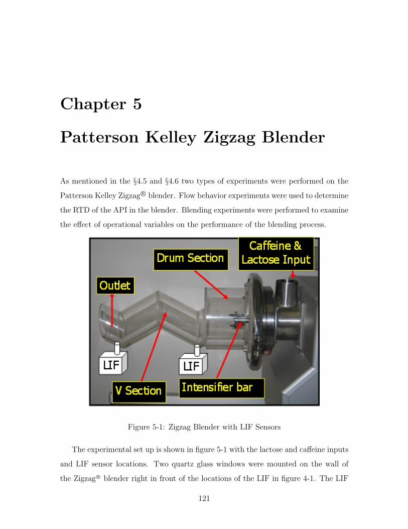
Chapter 5
Patterson Kelley Zigzag Blender
As mentioned in the §4.5 and §4.6 two types of experiments were performed on the
Patterson Kelley Zigzag R© blender. Flow behavior experiments were used to determine
the RTD of the API in the blender. Blending experiments were performed to examine
the effect of operational variables on the performance of the blending process.
Figure 5-1: Zigzag Blender with LIF Sensors
The experimental set up is shown in figure 5-1 with the lactose and caffeine inputs
and LIF sensor locations. Two quartz glass windows were mounted on the wall of
the ZigzagR© blender right in front of the locations of the LIF in figure 4-1. The LIF
121

sensor was triggered by a metallic detector that triggered the proximity sensor of the
LIF unit. The data was collected on two computers that communicated with the RF
devices of the two LIF units separately.
Figure 5-2: Schematic of the Placement of NIR sensor on the Zigzag Blender, courtesy:Bart Johnson, Axsun Tech. Inc.
The experimental set up was slightly modified when LIF and NIR sensors were
incorporated at the end of the blender. As shown in figure 5-2 and 5-3, the NIR sensor
was placed beneath a quartz glass plate adjacent to the LIF sensor. An air nozzle
operated by a solenoid valve and controlled by a computer communicating with the
NIR sensor was placed above the quartz glass window as shown in figure 5-3. The
solenoid valve purged the quartz glass with a compressed air burst to remove the
powder from the surface of the quartz glass. This air purge was triggered after at 3
second delay of the NIR sensor scan. The total scan time (inclusive of the collection
of three spectra) of the NIR sensor was 5 seconds and hence the collection frequency
was 0.2 Hz.
122

Figure 5-3: NIR Setup on the Zigzag Blender
5.1 Flow Behavior Experiments
Investigation of flow behavior was done in two parts. In the first part, steady state
in the blender was confirmed. In the second part the flow behavior was determined
by RTD experiments.
5.1.1 Confirmation of Steady State
In all the residence time distribution experiments performed, the output from the
blender was collected for a period of 10 minutes and the mass of the powder collected
was measured. This was compared with the total flow rate fed into the blender. The
equivalence of the input and output flow rates was assumed to indicate achievement
of steady state.
5.1.2 RTD Experiments
Determination of flow behavior through residence time experiments were performed
with caffeine as the API and HMS Impalpable Lactose as the excipient. The total
throughput was fixed at 50 kg/hr and a shot of caffeine corresponding to 3% of the
lactose present in the blender over a period of 3× the mean residence time (estimated
from flow rate and theoretical fill volume from the vendor) was administered. The
concentration of the API at the end of the drum section and at the exit of the Zigzag R©
was monitored using an LIF sensor. The LIF sensor was configured in such a way
that it would be triggered when the quartz glass window described in §4.1 passes
directly in front of the LIF sensor collection window.
123

The intensifier bar rotation rate was varied between 1500 and 3000 RPM and the
external shell rotation rate was varied between 25 and 50 RPM. The concentration
of the API (caffeine) was changed from 1% to 3%. These three factors were changed
in a full factorial design, with one repeat and one center point. The LIF responses,
however, could not be converted to concentrations since a priori calibration of the
LIF signal with concentration was not carried out with the Zigzag R© blender.
5.1.3 Analysis of Data
In confirming achievement of steady state, the mass of the powder collected 15 minutes
after feeding the impulse shot of caffeine was collected for ten minutes. The flow rate
was computed and compared with the total mass flow rate through the blender.
Since, LIF calibration was not carried out on the impulse response data, raw
LIF data from those experiments were statistically regressed with an empirical res-
idence time distribution and these results were graphically presented to understand
the spread and dead volume in the blender. However, LIF data from blending was
used to determine the residence time distribution, by converting the blending data
from LIF to concentrations by using an exponential fit of the ratio of the LIF sig-
nal to the LIF signal for the pure excipient (0% API). The exponential calibration
parameters for each run were determined separately and the data was converted to
concentrations.
In order to model the residence time distribution at the exit of the Zigzag R© blender
two models were employed. The first model was a log-normal distribution that was
used for RTD obtained from impulse response experiments, shown in equation (5.1).
This empirical distribution was regressed statistically based on the observations on
the data.
E (θ) =1
θ σ√
2 πexp
(− (log(θ)− µ)2
2σ2
)(5.1)
Another RTD model was used for determining the residence time distribution
from blending data (from varying throughput experiments). This model consisted of
a plug flow (delay) and mixed flow (ideal) blender in series was used. It was expected
124

Figure 5-4: RTD of Plug Flow and Ideal Mixer in Series
that the drum section and the V-section would act as an ideal and plug flow blender
respectively. This is graphically depicted in 5-4 and the equation for this residence
time distribution is given in equation (5.2).
E (t) =1
τdexp
(−t− τv
τd
)(5.2)
where τd is the residence time in the drum section (corresponding to the residence
time in the ideal blender and τv is the residence time in the V-section of the blender.
5.2 Blending Experiments
Three sets of blending experiments were performed in the Zigzag R© blender. In the first
set, caffeine and HMS impalpable lactose were mixed while the operational variables
like shell and intensifier bar rotation rates and caffeine content in the blend were
varied in the experimental design. In the second set of experiments, caffeine and HMS
lactose were blended with variations in the overall throughput rate and external shell
rotation rate. In the final set of experiments, caffeine, lactose and magnesium sterate
were blended in the Zigzag R© blender.
125

5.2.1 Two Component Blending
Caffeine and HMS impalpable lactose were mixed in the Zigzag R© blender. Similar
to the residence time distribution experiments on the Zigzag R© blender, the total
throughput (flow) rate was maintained constant at 50 kg/hr. The angle of incline of
the blender was fixed at 0◦. In all two component blending experiments, 15 − 20 gm
samples at 3 minute intervals were collected at the exit of the blender. LIF sensor
was used to monitor the progress of the blending system.
5.2.1.1 Varying Rotation Rates
In this set of experiments, a 2-level, 3-factor full factorial experimental design was
created by changing the external shell rotation rate from 25 to 50 RPM, the internal
intensifier bar rotation rate 1500 to 3000 RPM and the caffeine content from 1% to
3% by weight. Two LIF sensors were placed as shown in figure 5-3, one at the end of
the drum section and one at the end of the V section. Quartz glasses were mounted
to let the UV light through the walls for exciting the powder. A metallic plate on the
blender triggered the LIF sensor to radiate the sample with UV light and collect the
ensuing fluorescent response. This ensured that the LIF collected one data point per
rotation of the blender.
15 to 20 g powder samples were collected at the exit of the blender. These were
weighed and dissolved in 500 mL of de-ionized water in the Distek R© dissolution sys-
tem. Lactose and caffeine are both soluble in water and the solution diluted 20×, 30×
and 40× depending on the expected concentration of caffeine in the powder mixture.
The expected concentrations of caffeine in the powder mixture were estimated from
the mean concentration of caffeine at steady state for samples collected at steady
state, 12× this mean concentration for samples collected during the transient period,
and 0% caffeine concentration for the samples collected before caffeine flow rate was
started and after the caffeine flow rate was cut off. The concentration of caffeine in
solution was determined by UV absorption spectroscopy using the calibration curve
described in §4.3.
126

5.2.1.2 Varying Throughput
In this set of experiments, a 3-level, 2-factor full factorial experimental design was
created by changing the external shell rotation rate between 37.5, 50 and 75 RPM
and the total throughput (flow rate) between 40, 50 and 60 kg/hr. The intensifier
bar rotation rate was fixed at 3000 RPM, so was the angle of incline at 0◦ and the
caffeine content at 3%. For this set of experiments, the powder was allowed to fall on
a quartz glass plate below which a LIF sensor was placed to collect the fluorescent
response as shown in figure 5-1. The calibration curve #3 in §4.3 and in table 4.1 was
used to convert LIF signal to caffeine content. The LIF sensor collection frequency
was set at 1 Hz.
15 − 20 g powder samples were collected at 3 minute intervals at the exit of the
blender. These samples were then weighed and dissolved in 500 mL of de-ionized wa-
ter in the Distek R© dissolution system. Similar to the experiments on varying rotation
rates, the solutions were diluted to 20×, 30× and 40× depending on the expected
concentration of caffeine in the powder mixture. The expected concentrations of caf-
feine in the powder mixture were estimated from the mean concentration of caffeine
at steady state for samples collected at steady state, 12× this mean concentration for
samples collected during the transient period, and 0% caffeine concentration for the
samples collected before caffeine flow rate was started and after the caffeine flow rate
was cut off. For some solutions, the linear range was achieved only at 80× the dilu-
tion in de-ionized water at dissolution. The concentrations of caffeine in the diluted
solutions were determined by UV absorption spectroscopy using the calibration curve
described in §4.3.
5.2.2 Three Component Experiments
Pharmaceutical dry powder blending involves mixing multiple components with dif-
ferent physical and chemical properties for various reasons. A continuous blender
should be able to blend multiple components simultaneously or sequentially as the
process demands. In order to investigate the effect of three-component mixing on the
performance of continuous blender, three components were blended in the Zigzag R©
127

blender.
Figure 5-5: Schematic of Three Component Mixing in Zigzag Blender
Caffeine and HMS Impalpable Lactose were used as the API and excipient and
magnesium stearate (MgSt) was used as the lubricant. The introduction of the lubri-
cant was decided to be carried out at the end of the drum section, i.e. at the interface
(connection joint) of the drum and the V-section. This decision was taken with the
prior knowledge that the lubricant would overcoat the caffeine and lactose particles
causing a very strong potential for segregation. Therefore, the lubricant was made
not to see the drum section where the powder was fluidized and dispersed using the
intensifer bar. This arrangement is schematically shown in figure 5-5.
The concentrations of MgSt was varied between 0.5 and 1.5% In this set of exper-
iments, a 3 level, 2 factor full factorial experimental design was created by changing
the concentration of MgSt between 0.5%, 1% and 1.5% by weight and the external
shell rotation rate between 37.5, 50 and 75 RPM. The intensifier bar rotation rate was
fixed at 3000 RPM, the angle of incline at 0◦, the caffeine content at 3% by weight
and the total flow rate at 50 kg/hr.
NIR and LIF sensors were placed beneath a quartz glass plate near the exit of the
blender on which powder fell after exiting from the blender as shown in figure 5-3.
An air purge (blowing a gust of of compressed air) was connected via a solenoid value
which was triggered by the NIR sensor after a delay of 5 seconds from the time instant
of scanning the powder for NIR spectrum. Therefore, the frequency of sampling for
the NIR sensor was 0.2 Hz. The LIF sensor collection frequency was set to 1 Hz.
128

5.2.3 Analysis of Data
Different data analysis methodologies were carried out depending on the type of
experiments and the kind of data collected. LIF data were converted using a linear
calibration plot for the blending experiments where the caffeine content was varied
between 1% and 3% for different external shell rotation rates and internal intensifer
bar rotation rates.
5.2.3.1 Two Component Blending - Varying Rotation Rates
The experiments where external and internal rotation rates were varied, LIF data was
collected for caffeine contents of 1%, 1.5% and 3%. The steady state LIF signal values
for each of these concentrations were linearly regressed after subtracting the baseline
LIF signal at 0% caffeine that was obtained before caffeine flow rate was started into
the blender. This is done because of the fact that LIF signal at very small changes
in concentration is linear in nature. The linear calibration curve is specific to the
Zigzag R© blender experiments and was not used elsewhere.
Figure 5-6: Linear Calibration of Baseline Adjusted LIF signal on Zigzag Blender
The LIF sensors measures the fluorescence from caffeine and collects the signal as
a fraction of total collection capacity. This fraction can be calibrated to the caffeine
concentration. Generally, the LIF signal is non-linear over the entire range of 0 to
3%. However, within 1 to 3% the LIF signal can be approximated to linear if the
129
baseline is adjusted. Figure 5-6 shows this calibration line. Using this calibration
plot the LIF data can then be converted to caffeine concentrations at the position of
the LIF sensor.
The variance at the output was computed from the concentration data at steady
state obtained from LIF described above. The variance introduced at the input
was computed flow rate the data obtained from the Schenck Accurate Mechatron R©
feeders. The time stamped flow rate data were converted to mass fractions of caffeine
every second. This inlet data was used in computing the variance in the input caffeine
concentrations. The computed VRR ( = σ2in/σ
2out) was compared to a target variance
reduction where the outlet variance was set to an RSD = σtar
µ= 3%. Also, the RSD
was computed from the variance in the outlet caffeine concentration. The caffeine
concentrations obtained by dissolving the powder samples in water and running UV
spectroscopy were used in determining the VRR in the same manner.
A response surface model was used to determine the effect of independent op-
erational variables (external shell rotation rate and internal intensifier bar rotation
rates). On performing a response surface analysis on the dissolution assay data, a four
term second order model fitted the data within 5% level of significance. Tip speed
was found to interact with shell speed and shell speed was found to have a non-linear
(quadratic) influence. This response surface is shown in figure 5. The model equation
that was used to fit the data is given in equation (5.3).
V RR = A+B ·RPMshell+C ·Conc2caf +D ·RPM2shell+E ·RPMshell ·RPMint (5.3)
where A, B, C, D and E are constants whose sign determines the direction of
correlation (positive or negative) to the respective operational variables (or their
quadratic terms). The response surface was plotted as a function of the independent
variables, Conc and RPMshell for three different values of RPMint.
130

5.2.3.2 Two Component Blending - Varying Throughput
The experiments where the throughput rates were varied with fixed caffeine content
in all the runs, were analyzed by taking ratios of the observed LIF signal with the
LIF signal at 0% caffeine content. This ratio was exponentially calibrated with the
highest and lowest caffeine contents and the calibration curve so created for each
individual run was used in determining the caffeine concentrations. The time data of
caffeine concentrations was then used to determine RSD of the powder at the exit.
Caffeine concentrations from dissolution analysis of the powder samples collected in
the blending experiments were also used to determine RSD.
Since, response surface analysis with two factors (operational variables) changed
would have not have a serious statistical validity, a Principal Component Analysis of
the data matrix comprising of the operational variables (total throughput, external
shell rotation rate, total mean residence time, mean residence time in the drum and
v sections and the RSDs computed from LIF and dissolution assays) was carried out.
SIMCA-P+ (Umetrics Inc., Kinnelon, NJ) was used to perfrom the PCA analysis
and using this software, the first two principal component loadings were plotted in a
loadings bi-plot to assess the correlations between operational variables (independent
variables like total throughput and shell rotation rate and dependent variables like
residence times) and the observed RSD of caffeine at the exit of the blender. In
order to achive statistical accuracy, all the principal components till the number of
independent variables in each dataset were calculated and only the first two principal
components were utilized.
5.2.3.3 Three-component Blending
NIR and LIF data were collected from the three component blending experiments.
The data from LIF were converted to concentrations of caffeine by first taking the ratio
of the observed signal during blending to the LIF signal at 0% caffeine content. This
ratio was calibrated using an exponential calibration function between the highest
concentration (5%) and lowest (0%) concentration of caffeine and corresponding signal
ratios at these two concentrations. The calibration function was then used to convert
131

the LIF signals to concentrations and RSD at steady state for LIF was determined.
This RSD was used in the principal component analysis described in this section later
on.
The collected NIR data were processed using SIMCA-P+ (from Umetrics Inc.,
Kinnelon, NJ). The spectra were first converted to have unit variance over all the
wavelengths for each spectrum. These univariate spectra were then transformed by
taking a 11 point Savitzky-Golay first derivative and were normalized using the Stan-
dard Normal Variate (SNV) spectral transform. These transforms are regularly used
in the literature and have been discussed in detail elsewhere [64, 7].
The transformations used here remove two important sources of noise in the spec-
tral data. The first source arises from the variations in the density and particle size
of the powder in the NIR scan area. It was studied that changes in particle size and
density shifted baselines and offsets in NIR spectra. First derivative transformations
removed these baseline shifts. SNV transformation normalized all the spectra to a
unit variance within each wavelength.
Pure component spectra of MgSt, caffeine and lactose were taken at the end of
all the three component blending experiments on the Zigzag R© blender on the quartz
glass plate. The aforementioned transformations on the spectra were carried out on
the entire set of blending spectra and pure component spectra.
Figure 5-7: Computation of Spectral RSD from Principal Component Analysis
132

On computing first three principal components of the spectral data over all the
experimental runs, it was observed that in general three components explained the
variance in the spectra to about 95 − 99%. The loadings curve of the first two
principal components indicated maxima over the peaks corresponding to caffeine and
magnesium stearate spectral loading curve respectively. This indicated that the first
two principal components represented chemometric contributions from caffeine and
MgSt and hence were used in determining the spectral RSD.
The spectral RSD was computed by calculating the variance in the principal com-
ponent score corresponding to caffeine (first component) and subtracting the variance
observed at the 0% caffeine. The square root of this variance was divided by the ab-
solute value of the difference between the mean principal component score observed
at 0% caffeine and mean principal component score observed at steady state. The
spectral RSD computed this way shown in figure 5-7, was expected to reflect the real
chemometric RSD of caffeine in the mixture, since the errors arising from density
and particle size fluctuations were removed by the spectral transformations. The ex-
act same procedure was followed for determining the RSD of MgSt and the second
principal component score was used to determine the spectral RSD of MgSt.
133

134

Chapter 6
Zigzag Blender Performance
Data from the flow behavior and blending experiments on the Zigzag R© blender were
analyzed as discussed in the last chapter. The residence time distributions at the
drum and the exit were plotted with shell rotation rate, intensifer bar rotation rate
and caffeine content as parameters. The effects of each of these variables was studied.
6.1 Results of Flow Behavior Experiments
Flow behavior experiments consisted mainly of residence time distribution exper-
iments. Residence time distributions were computed from both impulse response
experiments and blending experiments for varying throughput rate experiments as
described in the previous chapter. The effect of external shell rotation rate, internal
intensifier bar and caffeine content is described in the sections below.
6.1.1 Confirmation of Steady State
Steady state in flow rate was achieved within the first ten minutes of the blending run.
The flow rates of material at the exit of the blender 15 minutes into the experimental
run was observed to vary within 3 − 5% of the nominal total throughput. This
balance of flow rates indicated that steady state was indeed achieved in the blender.
Fill weights could not be measured in the blender due to engineering problems in
weighing the blender in real time.
135
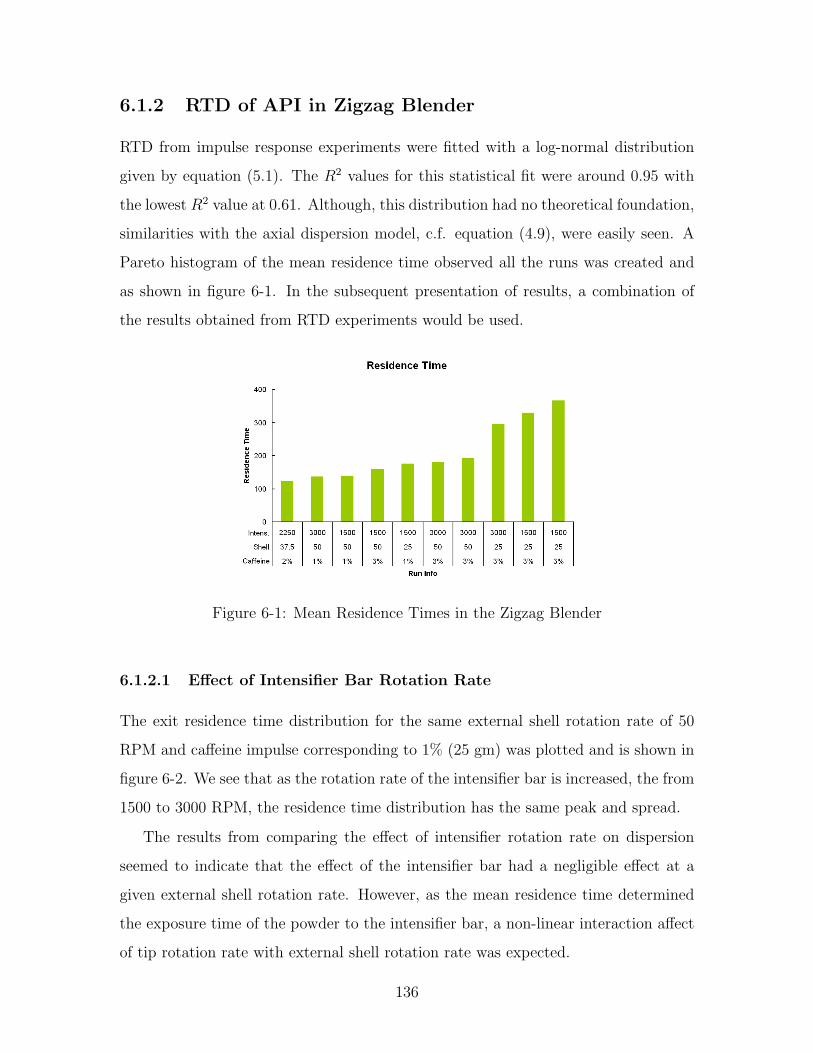
6.1.2 RTD of API in Zigzag Blender
RTD from impulse response experiments were fitted with a log-normal distribution
given by equation (5.1). The R2 values for this statistical fit were around 0.95 with
the lowest R2 value at 0.61. Although, this distribution had no theoretical foundation,
similarities with the axial dispersion model, c.f. equation (4.9), were easily seen. A
Pareto histogram of the mean residence time observed all the runs was created and
as shown in figure 6-1. In the subsequent presentation of results, a combination of
the results obtained from RTD experiments would be used.
Figure 6-1: Mean Residence Times in the Zigzag Blender
6.1.2.1 Effect of Intensifier Bar Rotation Rate
The exit residence time distribution for the same external shell rotation rate of 50
RPM and caffeine impulse corresponding to 1% (25 gm) was plotted and is shown in
figure 6-2. We see that as the rotation rate of the intensifier bar is increased, the from
1500 to 3000 RPM, the residence time distribution has the same peak and spread.
The results from comparing the effect of intensifier rotation rate on dispersion
seemed to indicate that the effect of the intensifier bar had a negligible effect at a
given external shell rotation rate. However, as the mean residence time determined
the exposure time of the powder to the intensifier bar, a non-linear interaction affect
of tip rotation rate with external shell rotation rate was expected.
136
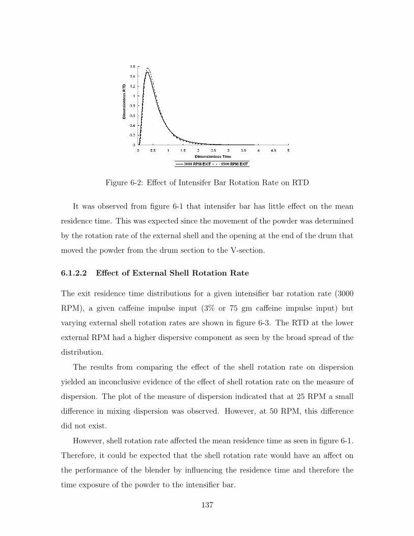
Figure 6-2: Effect of Intensifer Bar Rotation Rate on RTD
It was observed from figure 6-1 that intensifer bar has little effect on the mean
residence time. This was expected since the movement of the powder was determined
by the rotation rate of the external shell and the opening at the end of the drum that
moved the powder from the drum section to the V-section.
6.1.2.2 Effect of External Shell Rotation Rate
The exit residence time distributions for a given intensifier bar rotation rate (3000
RPM), a given caffeine impulse input (3% or 75 gm caffeine impulse input) but
varying external shell rotation rates are shown in figure 6-3. The RTD at the lower
external RPM had a higher dispersive component as seen by the broad spread of the
distribution.
The results from comparing the effect of the shell rotation rate on dispersion
yielded an inconclusive evidence of the effect of shell rotation rate on the measure of
dispersion. The plot of the measure of dispersion indicated that at 25 RPM a small
difference in mixing dispersion was observed. However, at 50 RPM, this difference
did not exist.
However, shell rotation rate affected the mean residence time as seen in figure 6-1.
Therefore, it could be expected that the shell rotation rate would have an affect on
the performance of the blender by influencing the residence time and therefore the
time exposure of the powder to the intensifier bar.
137

Figure 6-3: Effect of Shell Rotation Rate on RTD
6.1.2.3 Effect of Caffeine Content
The exit residence time distributions for a given intensifier bar rotation rate (3000
RPM) and a given external shell rotation rate of 50 RPM but two different caffeine
impulse inputs (3% or 75 gm and 1% or 25 gm caffeine impulse inputs) are shown
in firure 6-4. The RTD at both the levels of caffeine showed no significant difference
as evinced by the spreads of the two RTDs. When the measure of dispersion, given
by (σ2/t2m), was plotted vis-a-vis the caffeine impulse input loading for differing shell
rotation rates (25 and 50 RPM) and intensifier bar rotation rates (1500 and 3000
RPM), the difference observed was not significant.
Figure 6-4: Effect of Caffeine Content on RTD
138

The results from comparing the effect of caffeine content on the measure of disper-
sion seemed to indicate either negligible effect or lack thereof within the experimental
variance. However, higher caffeine contents required longer clearance times as seen
in figure 6-1. Therefore, it could be expected that the caffeine content would have
an affect on the performance of the blender by influencing the residence time and
therefore the time exposure of the powder to the intensifier bar. Also, API content is
inversely proportional to the RSD of the powder mixture and hence a higher variance
in mixtures with higher caffeine content would still give acceptable mixtures. In other
words, it would be easier to mix caffeine at 3% than caffeine at a concentration of 1%
since the equal RSD for both mixtures allows higher variance in 3% mixture than the
1% mixture.
6.1.2.4 Artefacts of the LIF Data Collection Method
The technique employed to measure LIF signal introduced errors in the data collected.
Due to the geometry of the blender, the LIF sensor was placed close to the quartz
glass windows in the Zigzag R© blender shown in the figure 5-1, on one side of the
blender. This arrangement caused two important errors.
1. It was observed that in consequent rotations of the external shell, the pow-
der layer varied in depth and thickness on the quartz glass. This error was
suspected when the observation that some rotations went past the LIF sensor
without complete powder coverage was made. The reason for this variation in
the depth of the quartz glass arises from the fact that powder moves in cascades
or avalanches in the V-section of the Zigzag R© blender causing powder to fall
erratically on the quartz window.
2. It was observed that the powder layer in contact with the quartz glass window
was not being replenished during subsequent rotations of the Zigzag R© blender.
This observation was made, only after the LIF data were collected. The LIF
data collected and a statistical log-normal curve-fit is shown in figure 6-5. This
example showed that a number of LIF scans passed before powder replenished on
139

Figure 6-5: Experimental RTD and Log-Normal Statistical Regression in ZigzagBlender
the quartz glass window as evinced by the static signal for about 3-5 rotations.
This static nature of the signal gave rise to additional errors in computing the
measure of dispersion in the blender using the log-normal RTD curve.
As a result of these issues, the RTD analyses from impulse-response experiments
were not expected to match the experimentally determined performance characteris-
tics of blending performance in the Zigzag R© blender.
6.2 Results of Blending Experiments
LIF data and dissolution assay of powder samples were analyzed for determination of
the variance reduction in the Zigzag R© blender. The variance reduction ratios from LIF
and dissolution assays for two component blending and from NIR for three-component
systems were analyzed. Response surface analysis and Principal component analysis
was carried out on the VRR data for two component blender as described in §5.2.3.
6.2.1 Varying Rotation Rates in Two Component Blending
The VRRs from LIF data for two component (Caffeine + Lactose) blending were
plotted as a histogram as shown in figure 6-6 for all the experimental runs. The VRRs
from dissolution assay for two component blending Caffeine+Lactose were plotted as
a histogram as shown in figure 6-7.
140

Figure 6-6: VRR in Zigzag Blender from LIF data
These histograms were arranged in a Pareto format with the highest From both fig-
ures, it was found that the observed VRR was higher than the target VRR computed
as described in §5.2.3 for most of runs. It was also found that the higher intensifier
bar speed exceeded the target VRR compared to the lower intensifier speeds and that
the target was easily achieved at higher caffeine contents than at lower caffeine con-
tents. Response surface analysis provided a mathematical process of analyzing these
effects.
6.2.1.1 Response Surface Analysis of VRR
Equation (5.3) was statistically regressed with the VRR data obtained from dissolu-
tion. It was decided to use the dissolution data than the LIF data as the expected
error from the LIF data was higher than that in the dissolution assay data as dis-
cussed in the previous section. SAS (SAS Institute, Cary, NC) was used to perform
the statistical regression of the VRR from dissolution. ANOVA was performed and
the results were tablulated in 6.1. It was found that the model has a very high
significance Pr > F = 0.0005 � 0.05 at 95% level of confidence.
141

Table 6.1: ANOVA of Response Model
Source Sum of Squares F Pr > F
Model 537.1 42.9 0.0005
Error 15.6
Corrected Total 552.7
Since the model was found to be highly significant, the significance for individual
effects were calculated. The magnitude and direction of various effects, rotation rate
of the external shell RPMShell, rotation rate of the intensifier bar RPMint, caffeine
content Conc and their quadratic combinations of these effects as shown in equa-
tion (5.3), were tabulated in table 6.2.
Table 6.2: Statistics of Individual Effects on VRR
Variable Parameter Estimate t Pr > | t |
Intercept A 67.88 4.41 0.007
RPMshell B −4.17 −4.63 0.006
Conc2 C −3625.65 -2.43 0.060
RPM2shell D 0.052 4.32 0.008
RPMshell ·RPMint E 0.00023 11.34 < .0001
End of Table
All parameters were significant except the coefficient C, corresponding to the
effect of caffeine content. This effect failed the 95% test by a very small margin
and potentially could still be an important significant effect. Intensifier rotation rate
showed a positive effect and the external shell rotation rate showed a quadratic effect
on the variance reduction ratio.
142
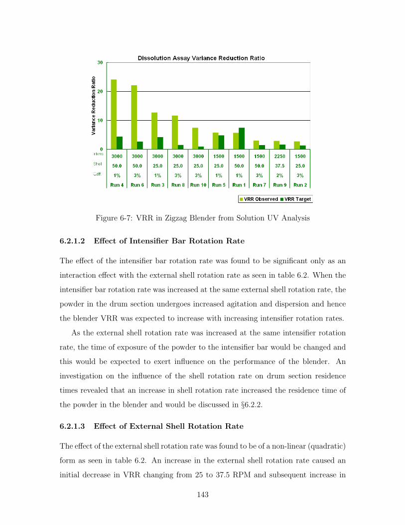
Figure 6-7: VRR in Zigzag Blender from Solution UV Analysis
6.2.1.2 Effect of Intensifier Bar Rotation Rate
The effect of the intensifier bar rotation rate was found to be significant only as an
interaction effect with the external shell rotation rate as seen in table 6.2. When the
intensifier bar rotation rate was increased at the same external shell rotation rate, the
powder in the drum section undergoes increased agitation and dispersion and hence
the blender VRR was expected to increase with increasing intensifier rotation rates.
As the external shell rotation rate was increased at the same intensifier rotation
rate, the time of exposure of the powder to the intensifier bar would be changed and
this would be expected to exert influence on the performance of the blender. An
investigation on the influence of the shell rotation rate on drum section residence
times revealed that an increase in shell rotation rate increased the residence time of
the powder in the blender and would be discussed in §6.2.2.
6.2.1.3 Effect of External Shell Rotation Rate
The effect of the external shell rotation rate was found to be of a non-linear (quadratic)
form as seen in table 6.2. An increase in the external shell rotation rate caused an
initial decrease in VRR changing from 25 to 37.5 RPM and subsequent increase in
143

changing from 37.5 to 50 RPM.
The non-linear effect of the external shell rotation rate was attributed to two
factors. First, as discussed above, a change in the external shell rotation rate changed
the residence time (increasing Shell RPM increased residence times) and second, a
change external shell rotation rates changed the dynamic angle of repose and thereby
changed the fill weight of the powder in the blender. It was found that these effects
worked to counterbalance each other and cause the non-linearity observed in the effect
of the external shell rotation rate.
6.2.1.4 Effect of Caffeine Content
The effect of caffeine content on VRR failed to be statistically significant at the 95%
level of statistical significance. However, an increase in the caffeine content was found
to decrease the variance reduction ratio. At the outset, this effect seemed to indicate
that increased caffeine content lead to decreased VRR. But theory indicated that
increase in concentration of the API should increase the VRR if the input variance
were identical.
Now, the feeder was known to perform better and introduce less variance at higher
concentrations. As a result of this effect from the feeder, VRR at higher concentra-
tions might have been lower. This was confirmed when we examined the difference of
Target and Observed VRRs shown in figures 6-6 and 6-7. This difference was higher
for 3% indicating that the performance was better at 3% since a higher difference
indicates a better reduction compared to the target variance.
6.2.2 Varying Throughput in Two Component Blending
Relative standard deviations (RSDs) of caffeine content for these blending experi-
ments were computed by converting LIF data to concentrations as described in §5.2.3.
These RSDs of caffeine content were plotted on a histogram as shown in 6-8. Caffeine
content were also determined from dissolving powder samples and subsequent UV
spectrometry on the samples. These concentrations were also used in determining
the RSD and were displayed graphically in a histogram format as shown in 6-9.
144

Figure 6-8: RSD of Caffeine from LIF - Throughput Experiments
Figure 6-9: RSD of Caffeine from Solution Analysis for Throughput Experiments
145

The correlation between the mean values and RSDs of caffeine content determined
from both these techniques were plotted as shown in figures 6-10 and 6-11. It was
found that RSDs computed from LIF and UV spectrometric analysis were very dif-
ferent. The mean values, however, had a very good correlation. Only three powder
samples at steady state were collected and this sample set did not give enough statis-
tical significance to the results from Dissolution analysis. As a result it was found that
the variance observed in the dissolution data were much larger than that observed in
the LIF data as shown in figure 6-11. Therefore, in the subsquent analyses, only the
RSD computed from LIF data were used.
Figure 6-10: Mean Caffeine Content: from LIF vs from Solution Analysis
6.2.2.1 PCA of RSD and Operational Variables
In order to understand the effect of operational variables on the RSD of the powder
mixture computed by converting LIF data to caffeine concentrations, principal com-
ponent analysis was performed as described in §5.2.3. Figure 6-12 the loadings plot
of various variables that affect the blending process. These are rotation rate of the
external shell, the total throughput rate, the mean residence time in the drum section
and the mean residence time in the V Section.
146

Figure 6-11: RSD of Caffeine: from LIF vs from Solution Analysis
Figure 6-12: Loadings Plot of Caffeine RSD - Rotation Rate and Total Flow Rate
147

6.2.2.2 Effect of External Shell Rotation Rate
The scalar product of the position vectors (from the origin in the loadings score plot)
of different variables on a loadings score plot determined the sign and extent of the
correlation between two variables. As the direction and magnitude of the position
vectors of The external shell rotation rate and RSD from LIF had positive scalar
product c.f. figure 6-12, the effect of Shell RPM on RSD of LIF within this experi-
mental design was positive. This meant that as rotation rate of the shell increased,
the RSD of caffeine increased or the quality of the mixture deteriorated.
Figure 6-13: Loadings Plot with RSD, Total Flow Rate, Mean Residence Times andShell Rotation Rate
In order to understand this effect, correlation between V-section residence time
and RPM was examined. From the figure, it was seen that these variables were
highly correlated, since the vectors have the same magnitude and direction. The
drum section, v section and total mean residence times were plotted as a function
of external shell rotation rates as shown in figure 6-13. Clearly this indicated that
an increase in the external shell rotation rate, increased the mean residence time in
the V-section causing an increase in the RSD of the powder mixture observed. Our
expectation was that as the residence time in the V-section increased, powder that
148

was mixed in the drum section began to segregate due to convective and gravity forces
and hence an increase in RSD was observed.
6.2.2.3 Effect of Total Throughput
The direction and magnitude of the position vectors of total flow rate and RSD
indicated that these variables were positively correlated. This meant that as the
total flow rate increased, the observed RSD from LIF data also increased.
To understand this, the effect of flow rate on drum section residence time was
observed. It was found that the drum section mean residence time and the flow rate
were negatively correlated. This meant that an decrease in the total flow rate caused
an increase in the drum section mean residence time which caused a decrease in the
RSD of the mixture due to reduced mixing time in the drum section.
6.2.3 Three Component Blending
Spectral RSDs that act as proxies for the actual RSDs of Magnesium Stearate and
Caffeine were computed as described in section §5.2.3. Since these RSDs were com-
puted on the principal components of transformed spectra, these did not represent
the real RSDs of the individual components, caffeine and MgSt. However, since
spectral data carried chemometric information, RSDs of the spectral principal com-
ponents were expected to reflect the trends in the RSDs of the individual component
concentrations in the powder mixture.
PCA was performed on different set of variables in order to understand the influ-
ence of different variables on the blending performance. PCA was performed on the
following sets of combinations of variables:
• Shell rotation rate, MgSt content and Caffeine spectral RSD.
• Shell rotation rate, MgSt content and MgSt Spectral RSD.
• Shell rotation rate, MgSt Content, MgSt Spectral RSD and Caffeine Spectral
RSD.
149
The effect of operational variables on these proxy spectral RSDs were investigated
by PCA analysis again described in §5.2.3. It is important to note that the spectral
RSDs in the results described below were all proxy RSDs computed from principal
components and are only a measure of the actual concentration RSD.
6.2.3.1 PCA of Spectral RSD with Shell Rotation Rate
As seen before, shell rotation rate had a positive effect of caffeine spectral RSD which
meant that as the rotation rate increased, the spectral RSD of Caffeine increased or
the blend quality deteriorated. In the two component blending scenario, increase in
shell rotation rate lead to an increase in V-section residence time and it was suspected
that the same effect was causing this correlation in these three component blending
experiments.
The effect of V-section mean residence time on the RSD computed from LIF
measurements made on the three component blending experiments shown in Figure
6-14 reinforce the results from the two component experiments c.f. figure 6-12. As
the V-section residence time increased, the spectral RSD of caffeine increased. Since
MgSt was introduced at the end of the drum section (i.e. after caffiene was mixed with
lactose in the drum section), and since MgSt lubricated particles by coating caffeine
and lactose with MgSt particles thereby decreasing cohesion and friction, the mixture
segregated in the V-section since the time of exposure to the tumbling section under
an increased segregation potential was more during its sojourn in the V-section.
6.2.3.2 Effect of MgSt on Caffeine RSD
The results from PC analysis of MgSt content on caffeine spectral RSD was plotted
on a loadings plot as shown in figure 6-14. It was found that the scalar product of
the position vectors of caffeine spectral RSD and MgSt content was positive which
indicated a positive correlation. In fact it was found that the position vectors were
approximately of same magnitude and in the same direction, which indicated that
these were very strongly correlated.
This effect of MgSt content on caffeine spectral RSD could be explained by the
150

Figure 6-14: Loading plot for Caffeine RSD, MgSt Content and Shell Rotation Rate
Figure 6-15: Loadings plot for MgSt RSD, MgSt Content, Caffeine RSD and ShellRotation Rate
151

microscopic behavior of how MgSt particles interact with caffeine and lactose par-
ticles. Caffeine and lactose particles were coated by fine MgSt particles during the
blending process in the V-section. MgSt coated caffeine and lactose particles lost
their cohesive and adhesive strength due to the reduced cohesion between MgSt -
Caffeine and MgSt - Lactose. This reduction in cohesion increased the potential for
lactose and caffeine particles to segregate in the V-section, where the only forces of
mixing were gravity forces, which increased segregation in the V-section. Increased
segregation resulted in a deteriorated mixture quality at the end of V-section (i.e.
higher caffeine spectral RSD).
6.2.3.3 Effect of MgSt on MgSt RSD
The results from PC analysis of MgSt content on MgST spectral RSD was plotted on
a similar loadings plot as before as shown in figure 6-15. It was found that the scalar
product of the position vectors of MgSt content and MgSt spectral RSD was positive
which indicated a positive correlation. The scalar product of the position vectors of
MgSt spectral RSD and shell rotation rate was found to be negative which indicated
a negative correlation.
It was expected that as MgSt content increased, the spectral RSD of MgSt would
decrease since RSD has a direct inverse proportionality with mean MgSt content.
However, the variance in MgSt content was found to exceed this inverse proportion-
ality leading to a positive correlation between MgSt content and MgSt RSD. It was
not clear if this was a result of preferential coating of MgSt on caffiene or lactose over
the other causing an increased spectral RSD.
The effect of RPM (which was positively correlated with the V-section residence
time) on the MgSt spectral RSD was positive, indicating that an increased residence
time in the V-section decreased the spectral RSD of MgSt, i.e, gave rise to a better
blend homogeneity with respect to MgSt RSD. However, at this point it was foreseen
that an increase in shell RPM would decrease the spectral RSD of MgSt, but might
cause problems with caffeine spetral RSD and this is discussed below.
152

6.2.3.4 Effect of MgSt RSD on Caffeine RSD
The results from PC analysis of MgSt content, MgSt spectral RSD and shell rotation
rate on caffeine spectral RSD was shown in a loadings plot in figure 6-15. It was
found that the scalar product of the position vectors of MgSt spectral RSD and
caffeine spectral RSD was negative which indicated a negative correlation between
the lubricant and API RSD.
As MgSt spectral RSD increased, the spread of MgSt in the powder mixture
decreased. This meant that fewer caffeine and lactose particles were coated with MgSt
thereby maintaining the cohesive and adhesive forces between caffeine and lactose at
their original levels leading to retained blend homogeneity in caffeine at the end of
the blender or in other words a decreased spectral RSD of caffeine.
We also observed that an increase in RPM (which lead to an increase in the
residence time in the V-section) decreased the spectral RSD of MgSt but increased
the spectral RSD of caffeine. In other words, increased time spent in the V-section
deteriorated the mixture quality in terms of caffeine spectral RSD, but increased the
spread of MgSt as evinced by decreased spectral RSD of MgSt with increased RPM
of the shell.
6.3 Summary of Results
The Zigzag R© blender was shown to exceed the performance achievable in batch blend-
ing. It was shown that the blending system could be monitored in real time using
a non-invasive technique like LIF. Effect of external shell rotation rate and internal
intensifier bar rotation rate, and total throughput of material through the blender
were also delineated. It was shown that residence time in the drum and V-sections
were affected by the shell rotation rates and flow rate of the material in the blender.
The effect of three component blending was also examined and it was shown that
lubricant like MgSt coult be monitored in real time. It was shown that the definition
of blend homogeneity with respect to one component in a multi-component blending
system does not necessarily mean homogeniety in another. In fact, it was shown that
153

an increase in RSD of the lubricant leads to a decrease in the RSD of the active. This
meant that there were trade-offs involved in the optimization of blending processes.
What could be good for one component need not necessarily be good for the rest of
the mixture.
Finally, a pilot scale Zigzag R© blender was tested and operated for blending two
and three component mixtures. It was shown that online monitoring of this system is
possible and that the blender and feeder system should be considered a single entity
while designing the blending process.
154
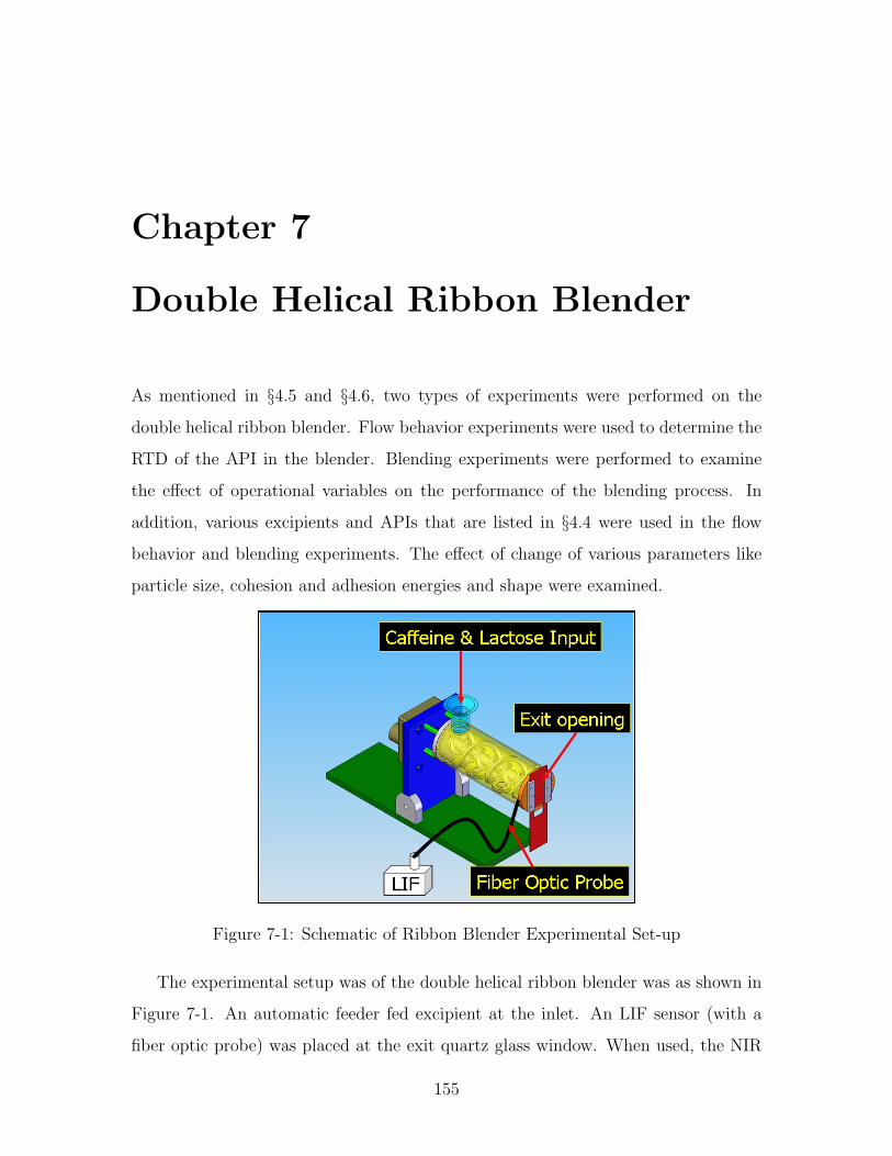
Chapter 7
Double Helical Ribbon Blender
As mentioned in §4.5 and §4.6, two types of experiments were performed on the
double helical ribbon blender. Flow behavior experiments were used to determine the
RTD of the API in the blender. Blending experiments were performed to examine
the effect of operational variables on the performance of the blending process. In
addition, various excipients and APIs that are listed in §4.4 were used in the flow
behavior and blending experiments. The effect of change of various parameters like
particle size, cohesion and adhesion energies and shape were examined.
Figure 7-1: Schematic of Ribbon Blender Experimental Set-up
The experimental setup was of the double helical ribbon blender was as shown in
Figure 7-1. An automatic feeder fed excipient at the inlet. An LIF sensor (with a
fiber optic probe) was placed at the exit quartz glass window. When used, the NIR
155
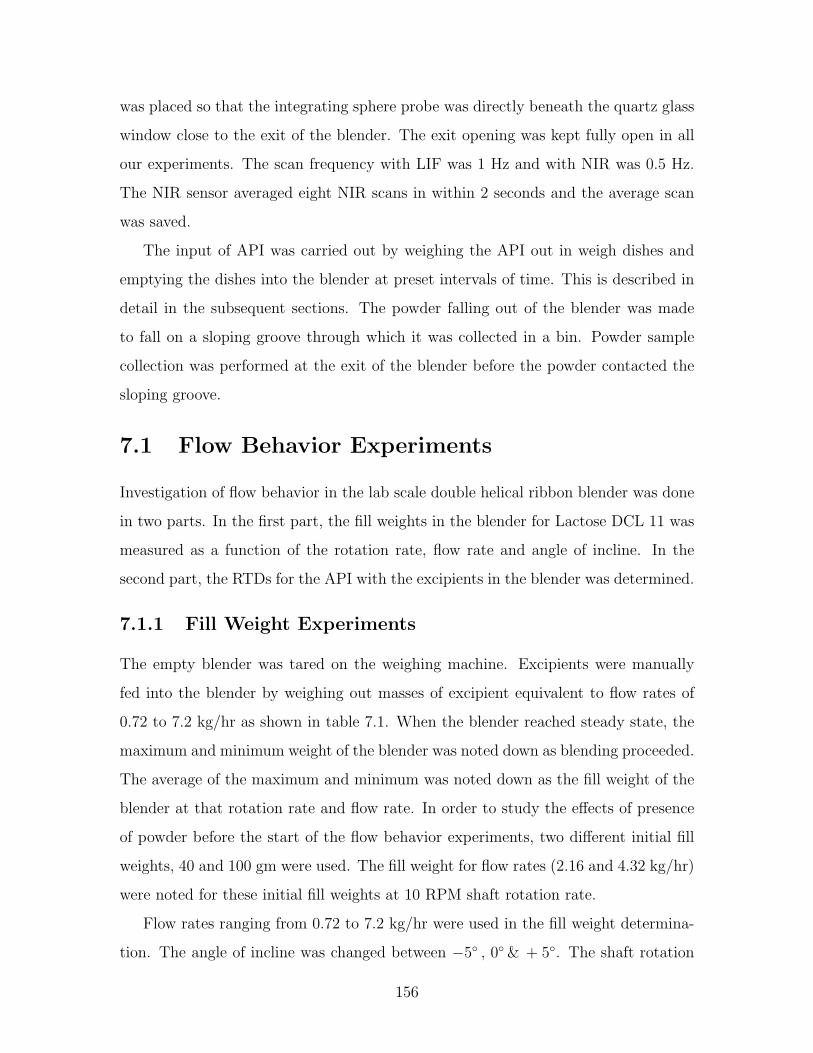
was placed so that the integrating sphere probe was directly beneath the quartz glass
window close to the exit of the blender. The exit opening was kept fully open in all
our experiments. The scan frequency with LIF was 1 Hz and with NIR was 0.5 Hz.
The NIR sensor averaged eight NIR scans in within 2 seconds and the average scan
was saved.
The input of API was carried out by weighing the API out in weigh dishes and
emptying the dishes into the blender at preset intervals of time. This is described in
detail in the subsequent sections. The powder falling out of the blender was made
to fall on a sloping groove through which it was collected in a bin. Powder sample
collection was performed at the exit of the blender before the powder contacted the
sloping groove.
7.1 Flow Behavior Experiments
Investigation of flow behavior in the lab scale double helical ribbon blender was done
in two parts. In the first part, the fill weights in the blender for Lactose DCL 11 was
measured as a function of the rotation rate, flow rate and angle of incline. In the
second part, the RTDs for the API with the excipients in the blender was determined.
7.1.1 Fill Weight Experiments
The empty blender was tared on the weighing machine. Excipients were manually
fed into the blender by weighing out masses of excipient equivalent to flow rates of
0.72 to 7.2 kg/hr as shown in table 7.1. When the blender reached steady state, the
maximum and minimum weight of the blender was noted down as blending proceeded.
The average of the maximum and minimum was noted down as the fill weight of the
blender at that rotation rate and flow rate. In order to study the effects of presence
of powder before the start of the flow behavior experiments, two different initial fill
weights, 40 and 100 gm were used. The fill weight for flow rates (2.16 and 4.32 kg/hr)
were noted for these initial fill weights at 10 RPM shaft rotation rate.
Flow rates ranging from 0.72 to 7.2 kg/hr were used in the fill weight determina-
tion. The angle of incline was changed between −5◦ , 0◦& + 5◦. The shaft rotation
156
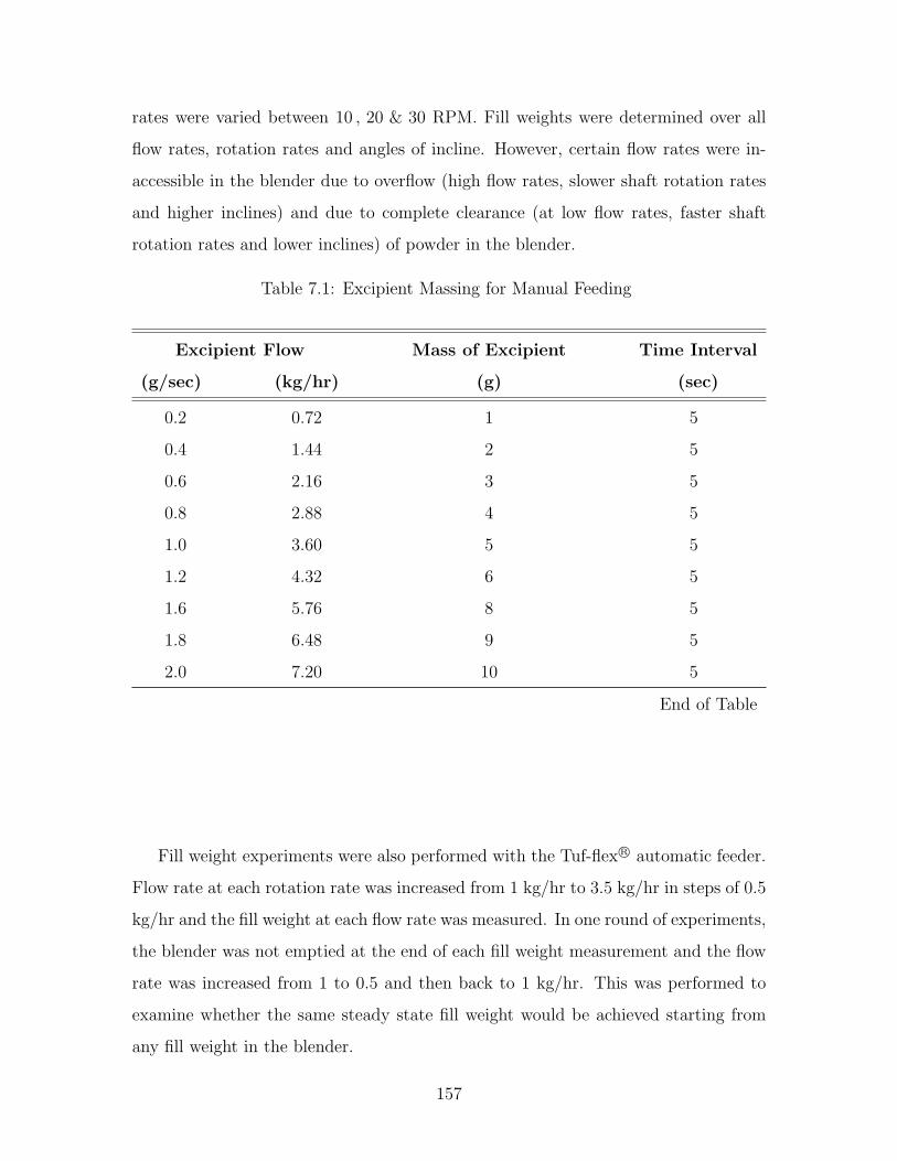
rates were varied between 10 , 20 & 30 RPM. Fill weights were determined over all
flow rates, rotation rates and angles of incline. However, certain flow rates were in-
accessible in the blender due to overflow (high flow rates, slower shaft rotation rates
and higher inclines) and due to complete clearance (at low flow rates, faster shaft
rotation rates and lower inclines) of powder in the blender.
Table 7.1: Excipient Massing for Manual Feeding
Excipient Flow Mass of Excipient Time Interval
(g/sec) (kg/hr) (g) (sec)
0.2 0.72 1 5
0.4 1.44 2 5
0.6 2.16 3 5
0.8 2.88 4 5
1.0 3.60 5 5
1.2 4.32 6 5
1.6 5.76 8 5
1.8 6.48 9 5
2.0 7.20 10 5
End of Table
Fill weight experiments were also performed with the Tuf-flex R© automatic feeder.
Flow rate at each rotation rate was increased from 1 kg/hr to 3.5 kg/hr in steps of 0.5
kg/hr and the fill weight at each flow rate was measured. In one round of experiments,
the blender was not emptied at the end of each fill weight measurement and the flow
rate was increased from 1 to 0.5 and then back to 1 kg/hr. This was performed to
examine whether the same steady state fill weight would be achieved starting from
any fill weight in the blender.
157
7.1.2 RTD Experiments
Determination of residence time distribution was carried out by perfroming impulse
response experiments. Before the installation of the feeder, manual feeding of both
the excipient and API was carried out by weighing out masses of excipient equivalent
to flow rates of 1.08, 2.16, 4.32 and 7.2 kg/hr. In each experiment, LIF monitoring
started at time t = 0. The excipients were weighed out in weigh boats and emptied
into the blender at regular, pre-determined intervals of time. Before the feeder was
installed, Lactose DCL 14 was used after sieving the powder so that two cuts were
obtained. The first cut had particle sizes between 45 and 150µm and the second cut
had particle sizes between 150 and 250µm.
The fill weight of the blender was noted at steady state, as the average between
the higher and lower values in the blender. The fill weight fluctuates in the blender
due to the discrete nature of powder flow at the exit and inlet of the blender. The
space time for the blender was estimated by dividing the fill weight at steady state
with flow rate at the inlet.
A shot of API (Caffeine in this case) corresponding to 3% by mass of the powder in
the blender over 3× the mean residence time (using τ , the space time, as an estimate
of mean residence time) was fed at the inlet of the blender and the time of the impulse
shot was noted. LIF signal was collected at a frequency of 1 Hz and was converted
to concentrations using the calibration curve #2 from table 4.1. The concentrations
were converted to residence time distributions using two different methods discussed
in §7.1.3.
An automatic feeder was installed to feed the excipient at the inlet of the blender.
The feeder delivered flowrates between 1 to 10 kg/hr. Lactose DCL-11, Lactose DCL-
14, MCC Avicel PH-102, and MCC Celphere CP-102 were used as excipients in this
set of experiments. Caffeine and Acetaminophen were used as two different APIs.
NIR monitoring in each experiment started at t = 0. The fill weight of the blender
was noted at steady state, as the average between the higher and lower values in the
blender. The fill weight fluctuates in the blender due to the discrete nature of powder
158

flow at the exit and inlet of the blender. The space time for the blender was estimated
by dividing the fill weight at steady state with flow rate at the inlet.
A shot of API (Caffeine or Acetaminophen) corresponding to 3% by mass of the
powder in the blender over 3× the mean residence time, (using τ , the space time, as
an estimate of mean residence time) was fed at the inlet of the blender and the time
of the impuse shot was noted. NIR spectra were collected at a frequency of 0.5 Hz
and these spectra were converted to concentration using the PLS models described in
§4.3. The angle of incline in the presence of the automatic feeder was fixed at 0◦. All
the types of excipients described in this chapter were used. The concentration were
subsequently converted to residence time distributions using the methods discussed
in §4.5.
7.1.3 Analysis of Data
The fill weight data was used to compute the space times in the blender. The impulse
response data were used to compute the Bodenstein number and mean residence time.
These methods of analysis of data are described below.
7.1.3.1 Fill Weight Experiments
The average fill weights in the blender at a particular flow rate, rotation rate and
angle of incline, were used in computing the space time. Space time was computed
by dividing the fill weight at steady state in the blender by the flow rate at the inlet.
These space times were used to determine the API shot corresponding to 3% by mass
of the powder in the blender over 3× the space time in the blender.
The fill weights were plotted as a function of the shaft rotation rates, the flow
rates and angles of incline to examine the effect of each of these variables. The effect
of initial fill weight was also examined. The steady state fill weights for the same flow
rates were plotted for different initial weights. Also, a closed loop of changing initial
fill weights based on the steady state fill weight achieved by an earlier flow rate was
plotted.
159

7.1.3.2 Residence Time Distribution
The LIF data from impulse response experiments were converted to concentration
using calibration #1 in table 4.1. The converted concentrations were then converted
to residence time distribution using equation (4.10) and (4.11). The residence time
distribution was normalized using the space time and the subsequent dimensionless
residence time was statistically regressed with equation (4.9). In this regression, the
Bodenstein numbers for each of the experiments were determined. The dispersion
coefficients were determined using the length of the blender L = 6′′ and mean velocity
of the powder in the blender V = Lτ, where τs is the space time in the blender.
The NIR data were first pre-processed by taking 11-point Savitszky-Golay first
derivative followed by a standard normal variate transform described in §4.3. The pre-
processed data were converted to concentration of the API using the PLS calibration
models from SIMCA-P+ given summarized in table 4.2. The converted concentrations
were directly regressed with equation (4.12) to obtain the parameters A, τ , Bo.
A principal component analysis using SIMCA-P+ was carried out on the Boden-
stein number along with the mean residence time and rotation rate, fill weight and
the types of excipients and API. It was expected that this analysis would yield the
effect of particle and operational parameters on the bodenstein number and mean
residence time.
7.2 Blending Experiments
Powder blending experiments were performed in two sets. In the first set, two com-
ponent blending experiments were carried out in the ribbon blender. Both Caffeine
and Acetaminophen were used in combination with Lactose DCL-11 and DCL-14
and MCC Avicel PH-102 excipients. In the second set, three component experiments
with magnesium stearate were examined. Acetaminophen and caffeine were mixed
separately with Lactose DCL-11 and Magnesium Stearate (MgSt).
160
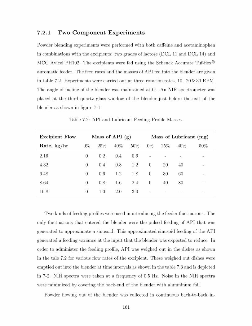
7.2.1 Two Component Experiments
Powder blending experiments were performed with both caffeine and acetaminophen
in combinations with the excipients: two grades of lactose (DCL 11 and DCL 14) and
MCC Avicel PH102. The excipients were fed using the Schenck Accurate Tuf-flex R©
automatic feeder. The feed rates and the masses of API fed into the blender are given
in table 7.2. Experiments were carried out at three rotation rates, 10 , 20 & 30 RPM.
The angle of incline of the blender was maintained at 0◦. An NIR spectrometer was
placed at the third quartz glass window of the blender just before the exit of the
blender as shown in figure 7-1.
Table 7.2: API and Lubricant Feeding Profile Masses
Excipient Flow Mass of API (g) Mass of Lubricant (mg)
Rate, kg/hr 0% 25% 40% 50% 0% 25% 40% 50%
2.16 0 0.2 0.4 0.6 - - - -
4.32 0 0.4 0.8 1.2 0 20 40 -
6.48 0 0.6 1.2 1.8 0 30 60 -
8.64 0 0.8 1.6 2.4 0 40 80 -
10.8 0 1.0 2.0 3.0 - - - -
Two kinds of feeding profiles were used in introducing the feeder fluctuations. The
only fluctuations that entered the blender were the pulsed feeding of API that was
generated to approximate a sinusoid. This approximated sinusoid feeding of the API
generated a feeding variance at the input that the blender was expected to reduce. In
order to administer the feeding profile, API was weighed out in the dishes as shown
in the tale 7.2 for various flow rates of the excipient. These weighed out dishes were
emptied out into the blender at time intervals as shown in the table 7.3 and is depicted
in 7-2. NIR spectra were taken at a frequency of 0.5 Hz. Noise in the NIR spectra
were minimized by covering the back-end of the blender with alumninum foil.
Powder flowing out of the blender was collected in continuous back-to-back in-
161

Figure 7-2: Input Fluctuations of API Content to the Ribbon Blender
tervals of 10 s each for one run at each rotation rate. This process yielded about 5
to 10 gm of powder in the sample vials. The spectra of these powder samples were
taken offline by placing the sample vial on the NIR sensor window and scanning the
NIR spectrum (after taking a background with the Spectralon tablet inside the vial).
This process gave an averaged concentration of the API in a powder sample corre-
sponding to 3× the dose size that the FDA requires for validation of the blending
process. Hence offline spectra of these powder samples were expected to reflect the
blend quality as required by the FDA.
Table 7.3: API Feeding Time Profiles
Profile Time Period Time Instant Concentration
0s 0%
5s 25%
Normal Peak 25s10s 40%
15s 40%
20s 25%
Continued on next page...
162

Profile Time Period Time Instant Concentration
25s 0%
0s 0%
10s 25%
20s 40%
Extended Peak 60s 30s 50%
40s 40%
50s 25%
60s 0%
End of Table
7.2.2 Three Component Experiments
Magnesium stearate (MgSt) was blended in the continuous blender with both active
ingredients caffeine and acetaminophen with the excipient DCL-11 in three component
blending experiments. The active ingredients were weighed out according to the Mass
of API column in table 7.2 and corresponding lubricant masses was added on top of
the active ingredient according to the Mass of lubricant column in the same table.
The lubricant masses corresponded to a concentration of 1.5% of magnesium stearate
by mass.
The Normal peak time profile feeding from table 7.3 was followed in feeding the
API and lubricant that had been weighed out together in the same weigh boats.
Only one rotation rate of the shaft - 10 RPM - was used for both caffeine and ac-
etaminophen. Excipient Lactose DCL-11 was fed in accordance to the feed rates
mentioned in table 7.3. Magnesium stearate was weighed out in dishes along with
caffeine or acetaminophen, whichever was the API, in accordance to the masses given
in the table 7.3. These dishes were emptied out to the blender at a frequency corre-
sponding to the normal peak wave (Tf = 25s) in intervals of 5 seconds.
NIR spectra of the powder at the quartz glass window closest to the exit was col-
lected. Powder samples were also collected in a fashion similar to the two component
163
experiments. One set of powder samples corresponding to each rotation rate were
collected for both the APIs. These powder samples were equivalent to 3× the dose
size of the tablet as mandated by the FDA. Hence offline spectra of these powder
samples were expected to reflect the blend quality as required by the FDA.
7.2.3 Analysis of Data
The PLS calibration method was used to convert the NIR data to concentrations.
Variance reduction ratios were computed based on these concentrations. In order to
address the effect of scale of scrutiny a 15 point moving average model was used to
smooth the data. These methods and reasoning behind utilising these methods of
analysis of data is described below.
7.2.3.1 Two Component Blending
Just like the NIR data from impulse response experiments, the NIR data were first pre-
processed by taking 11-point Savitszky-Golay first derivative followed by a standard
normal variate transform described in §4.3. The pre-processed data were converted
to concentration of the API using the PLS calibration models from SIMCA-P+ given
summarized in table 4.2.
Variance reduction ratio was computed by dividing the input variance by the the
variance of 100 sample points at steady state computed by converting the NIR spectra
to concentrations. Theoretical variance reduction ratio was computed using equation
(4.25). The random mixture variance was computed by calculating the number of
particles that the NIR spectrometer scans in each scan. The diameter of the NIR
spectrometer scan window was 1mm. The penetration depth was known to be close
to 2mm. With this estimate, the number of particles was computed using the particle
size distribution of the excipients and API was found to be 12, 000. Using this as the
number of particles in equation (4.22), the random mixture variance was determined
and used in computing the theoretical variance reduction ratio.
The number of points in the moving average model was determined as follows. The
mass of powder examined at each NIR scan was determined. The size of the scan
164
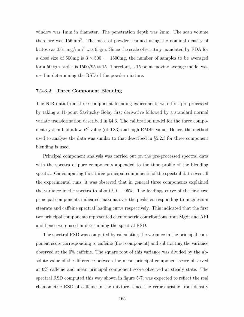
window was 1mm in diameter. The penetration depth was 2mm. The scan volume
therefore was 156mm3. The mass of powder scanned using the nominal density of
lactose as 0.61 mg/mm3 was 95gm. Since the scale of scrutiny mandated by FDA for
a dose size of 500mg is 3 × 500 = 1500mg, the number of samples to be averaged
for a 500gm tablet is 1500/95 ≈ 15. Therefore, a 15 point moving average model was
used in determining the RSD of the powder mixture.
7.2.3.2 Three Component Blending
The NIR data from three component blending experiments were first pre-processed
by taking a 11-point Savitszky-Golay first derivative followed by a standard normal
variate transformation described in §4.3. The calibration model for the three compo-
nent system had a low R2 value (of 0.83) and high RMSE value. Hence, the method
used to analyze the data was similar to that described in §5.2.3 for three component
blending is used.
Principal component analysis was carried out on the pre-processed spectral data
with the spectra of pure components appended to the time profile of the blending
spectra. On computing first three principal components of the spectral data over all
the experimental runs, it was observed that in general three components explained
the variance in the spectra to about 90 − 95%. The loadings curve of the first two
principal components indicated maxima over the peaks corresponding to magnesium
stearate and caffeine spectral loading curve respectively. This indicated that the first
two principal components represented chemometric contributions from MgSt and API
and hence were used in determining the spectral RSD.
The spectral RSD was computed by calculating the variance in the principal com-
ponent score corresponding to caffeine (first component) and subtracting the variance
observed at the 0% caffeine. The square root of this variance was divided by the ab-
solute value of the difference between the mean principal component score observed
at 0% caffeine and mean principal component score observed at steady state. The
spectral RSD computed this way shown in figure 5-7, was expected to reflect the real
chemometric RSD of caffeine in the mixture, since the errors arising from density
165

and particle size fluctuations were removed by the spectral transformations. The ex-
act same procedure was followed for determining the RSD of MgSt and the second
principal component score was used to determine the spectral RSD of MgSt.
166

Chapter 8
Ribbon Blender Performance
The experiments described in chapter 7 and the analysis described in §7.1.3 and §7.2.3
were carried out. The effect of operational variables like shaft rotation rate, flow rate
of excipient, angle of incline on the flow behavior and blending performance were
studied.
8.1 Results on Flow Behavior Experiments
The steady state fill weight suggested a dependence on the initial fill weight in the
blender. In order to establish qualify this dependence, the steady state fill weights
were determined by running the blender in a cycle from 1 kg/hr to 3.5 kg/hr and then
back to 1 kg/hr in a loop. From the RTD data, strong effects on mean residence time
were detected from shaft rotation rate and flow rate, but insignificant dependence of
Bodenstein number on operational variables was detected.
8.1.1 Fill Weight Experiments
Fill weight experiments were performed in the presence and absence of the automatic
excipient feeder. In the absence of the automatic feeder, the effect of inital fill weight
was examined by setting different initial fill weights. When the automatic feeder was
used, a cycle experiment where the flow rate was increased from 1 to 3.5 kg/hr and
then back to 1 kg/hr was performed as described in the chapter 7.
When the blender was manually fed, the fill weight fluctuated between a maximum
and a minimum. This fluctuation was also seen in the evolution of flow rate with
167
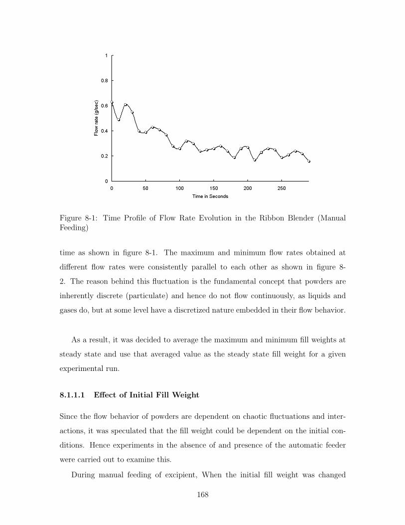
Figure 8-1: Time Profile of Flow Rate Evolution in the Ribbon Blender (ManualFeeding)
time as shown in figure 8-1. The maximum and minimum flow rates obtained at
different flow rates were consistently parallel to each other as shown in figure 8-
2. The reason behind this fluctuation is the fundamental concept that powders are
inherently discrete (particulate) and hence do not flow continuously, as liquids and
gases do, but at some level have a discretized nature embedded in their flow behavior.
As a result, it was decided to average the maximum and minimum fill weights at
steady state and use that averaged value as the steady state fill weight for a given
experimental run.
8.1.1.1 Effect of Initial Fill Weight
Since the flow behavior of powders are dependent on chaotic fluctuations and inter-
actions, it was speculated that the fill weight could be dependent on the initial con-
ditions. Hence experiments in the absence of and presence of the automatic feeder
were carried out to examine this.
During manual feeding of excipient, When the initial fill weight was changed
168

Figure 8-2: Maximum and Minimum Fill Weight at 10 RPM (Manual Feeding)
Figure 8-3: Dependence of Fill Weight on Initial Conditions
169

Figure 8-4: Steady State Fill Weights: Changing Initial Conditions with AutomaticFeeder
Figure 8-5: Repeatability of Fill Weights
170

from 40 gm to 100 gm the fill weight changed nominally as shown in figure 8-3. The
difference between the observed steady state fill weights at these two initial conditions
seemed quite small (only 6%.) The automatic feeder was used to feed lactose DCL
14 to the blender and a cycle experiment of increased and decreasing the flow rates
was performed. No considerable effect of changing initial fill weights in the blender
as shown in figure 8-4. Therefore, it was concluded that the scale of operation of the
blender did not give rise to fluctuations in the fill weights to a large extent. A repeat
experiment on determining fill weights showed that the linearity of fill weight was
very repeatable as shown in figure 8-5.
8.1.1.2 Effect of Flow Rate on Fill Weight
As flow rate was increased, the fill weight in the blender increased linearly as shown in
figures 8-5, 8-6, 8-7, and 8-8. This was in agreement with the fact that ribbon blender
was a moderate shear equipment and no deformation or particle size reduction causing
changes in density occured. Therefore, a linear change in the fill volume with flow rate
was expected. However, at +5◦ a change in the slope of the linear curve of fill weight
vs flow rate was observed at all rotation rates and this effect would be discussed later.
Figure 8-6: Steady State Fill Weights at Zero Degree Incline
171

8.1.1.3 Effect of Shaft Rotation Rate on Fill Weight
As the rotation rate increased, the fill weight in the blender decreased. This could
be explained due to the fact that as rotation rate increased, the rate of removal from
the blender increased causing a fall in the fill weight of the powder in the blender.
However, it was observed that all the three angles of incline did not show the same
effect with rotation rate and would be discussed below.
Figure 8-7: Steady State Fill Weights at -5 Degree Incline
8.1.1.4 Effect of Angle of Incline on Fill Weight
At 0◦ the fill weight linearity with flow rate had different X-intercepts at different
rotation rates as shown in figure 8-6. This was due to the fact at very low flow rates
the blender was cleared of all powder at 20 and 30 RPM causing X intercept to be
0 or positive. At 10 RPM the blender the fill weight of the blender was non-zero at
very low flow rates and this limit was shown to be 10% of the maximum fill weight
in the blender.
At−5◦ the fill weight linearity with flow rate had the same X-intercepts at different
rotation rates and was at 0% as shown in figure 8-7. This was due to the fact at very
172

Figure 8-8: Steady State Fill Weights at +5 Degree Incline
low flow rates the blender was cleared of all powder at all rotation rates causing X
intercept to be 0.
At +5◦ the fill weight linearity with flow rate changed slopes as flow rates increased
as shown in figure 8-8. The effect of 20 and 30 RPM were not very different above this
critical flow rate. It was observed that the second window of the blender (c.f. figures
4-2 and 7-1 became active and powder began flowing out of the second window. This
caused a reduction in the slope of the fill weight vs flow rate line as more flow rate
was required to achieve a certain fill weight after the critical flow rate.
8.1.2 RTD of API in Ribon Blender
The impulse response experimental data from LIF and NIR experiments were con-
verted to concentrations and the axial dispersion model was used to fit the data as
shown in figure 8-9. It was observed that this axial dispersion model could statistically
explain over 85% of the variance in all the observed data. Many of the experimental
RTDs had an R2 value of 0.9 or higher using the open-open axial disperion model
(c.f. equation (4.9)). The fitted values of Bo and τ were analyzed in terms of their
dependence on different operational parameters.
173
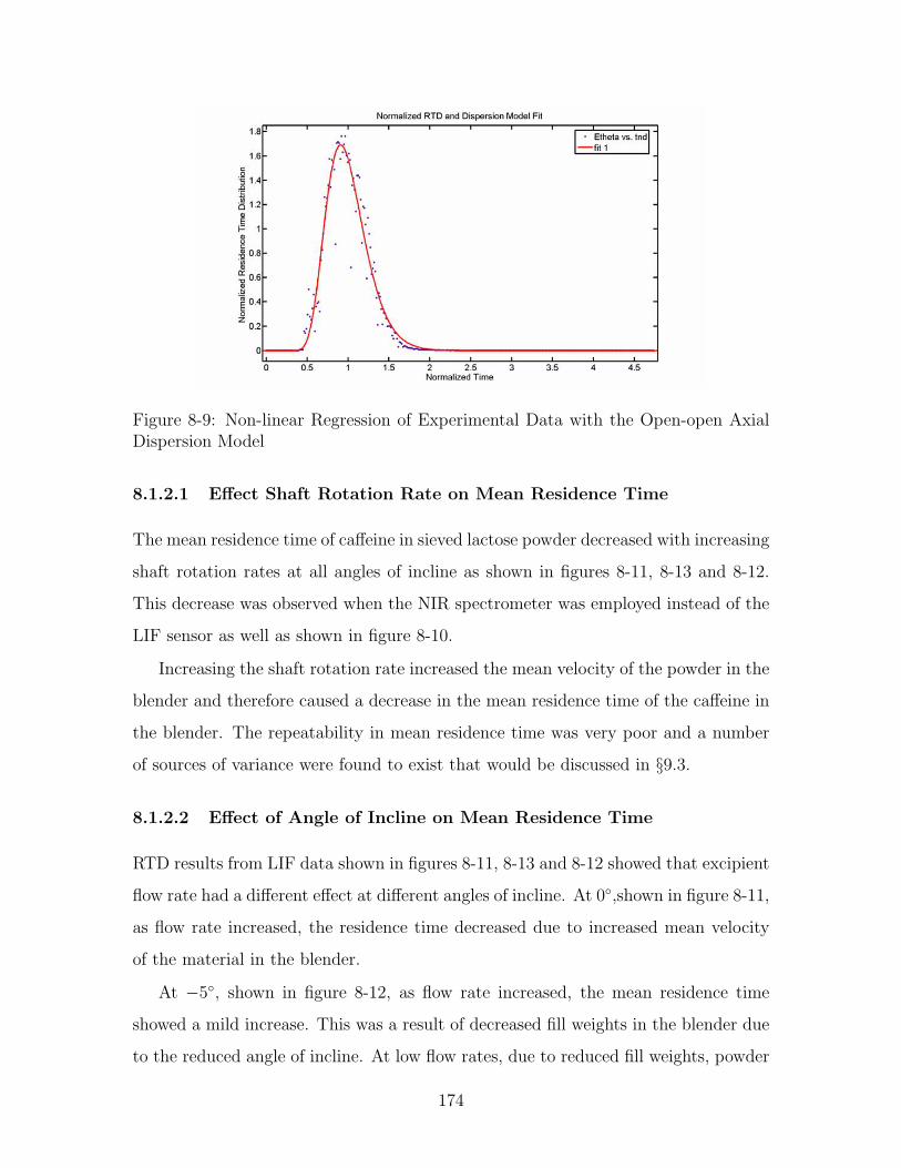
Figure 8-9: Non-linear Regression of Experimental Data with the Open-open AxialDispersion Model
8.1.2.1 Effect Shaft Rotation Rate on Mean Residence Time
The mean residence time of caffeine in sieved lactose powder decreased with increasing
shaft rotation rates at all angles of incline as shown in figures 8-11, 8-13 and 8-12.
This decrease was observed when the NIR spectrometer was employed instead of the
LIF sensor as well as shown in figure 8-10.
Increasing the shaft rotation rate increased the mean velocity of the powder in the
blender and therefore caused a decrease in the mean residence time of the caffeine in
the blender. The repeatability in mean residence time was very poor and a number
of sources of variance were found to exist that would be discussed in §9.3.
8.1.2.2 Effect of Angle of Incline on Mean Residence Time
RTD results from LIF data shown in figures 8-11, 8-13 and 8-12 showed that excipient
flow rate had a different effect at different angles of incline. At 0◦,shown in figure 8-11,
as flow rate increased, the residence time decreased due to increased mean velocity
of the material in the blender.
At −5◦, shown in figure 8-12, as flow rate increased, the mean residence time
showed a mild increase. This was a result of decreased fill weights in the blender due
to the reduced angle of incline. At low flow rates, due to reduced fill weights, powder
174

Figure 8-10: Mean Residence Times from NIR Data
Figure 8-11: Mean Residence Times (0◦)
175

Figure 8-12: Mean Residence Time (−5◦)
did not come in contact with the inner ribbon of the blender and hence the residence
time was lower than what was observed at 0◦ and 5◦. But as the flow rate increased
fill weights increased, which lead the powder to come in contact with the inner ribbon
thereby increasing the mean residence time of powder in the blender.
At +5◦, shown in figure 8-13, a similar phenomenon, as was observed in the fill
weights, was seen. The mean residence times increased from low flow rates to a
critical flow rate after which the the mean residence times began to decrease with
incresing flow rate. It was observed that this maximum occured at the point where
the second exit in the ribbon blender as shown in figures 4-2 and 7-1 was activated
and powder began flowing out of the second exit as well. After the second window
was active, the mean residence times began decreasing with increasing flow rate due
to increased mean velocities of the particles in the blender. As with the observations
on fill weights, 20 and 30 RPM were found to give similar mean residence times at
higher flow rates.
176

Figure 8-13: Mean Residence Times (+5◦)
8.1.2.3 Effect of Flow Rate on Mean Residence Time
Increasing Flow rate was expected to decrease the mean residence time of caffeine in
the blender. However, this effect was found to interact with the shaft rotation rate
and the angle of incline. When angle of incline was increased, a maximum in mean
residence time was observed near the critical flow rate where the second window was
activated. When the angle of incline was decreased, the inner ribbon was not activated
due to low fill weights and hence caused an increase in mean residence times as flow
rates increased. It was found that within a given regime of operation, increasing flow
rates decreased mean residence times due to increased mean velocities of particles in
the blender.
8.1.2.4 Effect Shaft Rotation Rate on Dispersion Coefficient
Dispersion coefficients were computed using experimentally determined mean resi-
dence times and Bodenstein numbers as described in §7.1.3. As rotation rates were
increased, the dispersion coefficient at +5◦ and −5◦ (c.f. figures 8-15 and 8-16) an-
gles of incline showed an increase at higher flow rates. This was attributed to the
increase in fill weight of the powder in the blender which resulted in increased mixing
177

by both the inner and outer helices. The overall effect of rotation rates on dispersion
coefficient at different angles of incline, however, was found to be inconclusive.
Figure 8-14: Dispersion Coefficient of Caffeine in Sieved Lactose (0◦ Incline)
8.1.2.5 Effect of Flow Rate on Dispersion Coefficient
The effect of flow rate, as seen in the graphs plotting dispersion coefficients with
flow rate and rotation rates for different angles of incline in figures 8-14, 8-15 and 8-
16, on dispersion coefficient was very negligilble. The disperion coefficient remained
independent of the flow rate over all the experiments.
8.1.2.6 Effect of Angle of Incline on Dispersion Coefficient
Decreasing the angle of incline from 0◦ to −5◦ was found to have a large effect of
dispersion coefficients. The dispersion coefficients at −5◦ and 30 RPM averaged at 1
cm2/s while at 0◦ and +5◦ the dispersion coefficients were considerably less ( ≈ 0.5
cm2/s) as seen by comparing figures 8-14, 8-15 and 8-16. However, the errors in
the estimating dispersion coefficients from the RTD are considerably higher, casting
doubts on the validity of this effect.
178
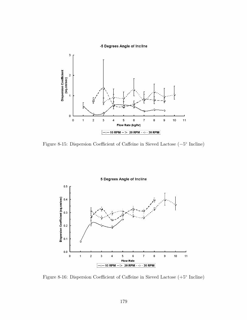
Figure 8-15: Dispersion Coefficient of Caffeine in Sieved Lactose (−5◦ Incline)
Figure 8-16: Dispersion Coefficient of Caffeine in Sieved Lactose (+5◦ Incline)
179

8.2 Results of Blending Experiments
Blending experiments were performed as described in chapter 7 and the data was
analyzed as described in §7.2.3. The angle of incline was fixed at 0◦ and the two exits
of the blender were completely opened for all the blending experiments. For the two
component experiments, the effect of rotation rate, time period of fluctuation and
mean residence time and dispersion coefficient on variance reduction ratio was ex-
amined. For the three component experiments, the comparison between the spectral
RSDs in the presence and absence of the third component was examined.
8.2.1 Two Component Experiments
Blending experiments were performed with three excipients, two APIs and at two
different feeding fluctuation frequencies. From the RTD experiments, it was gleaned
that the mean residence time was the factor that varied the most while dispersion
coefficient was predominantly invariant within many of the experiments. It was there-
fore expected that dispersion coefficient would have little effect on variance reduction
ratio within the range of experiments performed.
8.2.1.1 PCA of VRR
Principal component analysis of variance reduction ratio data, axial dispersion coeffi-
cients and mean residence times was performed on all the experiments. It was found
that the mean residence time had the strongest correlation with VRR as shown by
figure 8-17 where the position vector of the variable, VRR has a positive scalar prod-
uct with the position vector of mean residence time, indicating that a higher mean
residence time increases the variance reduction ratio. The scalar product of the po-
sition vector of dispersion coefficient is almost orthogonal to the position vector of
variance reduction ratio.
8.2.1.2 Effect of Dispersion Coefficient
The effect of dispersion coefficient was shown to be negligible on variance reduction
ratio in the experimental design space of the set of experiments performed in this
180

Figure 8-17: Loadings Plot of VRR, Mean Residence Time and Dispersion Coefficient
work. The reason behind this negligible effect can be reasoned out by taking recourse
to the fact that the dispersion coefficients in our work did not vary greatly, but were
bounded between 0.1 and 2 cm2/sec. Also, considering equations (4.9) and (4.25), it
was seen that such a small variation in dispersion coefficient would have very small
effect on the variance reduction ratio since variance reduction ratio was proportional
to√Bo exp−Bo which did not exhibit strong changes in VRR even though Bo varied
10× within the experimental space. However, as we shall see later, mean residence
time had a strong effect on VRR and also varied from 25 secs to 90 sec in our
experiments.
8.2.1.3 Effect of Shaft Rotation Rate
Principal component analysis of variance reduction ratio, shaft rotation rates, flow
rate, and fill weight and mean residence time was carried out. The resulting loading
plot showed that the variance reduction ratio has a negative correlation with the shaft
rotation rate and fill weight. This was evident from the negative scalar product of
the position vectors of VRR with shaft rotation rate and fill weight as shown in figure
8-18. As an aside, it was found that the shaft rotation rate correlated negatively with
181

the mean residence time and this was in agreement with the results from the RTD
analysis where an increase in shaft rotation rate resulted in decreased mean residence
times and fill weights.
Figure 8-18: Loadings plot of VRR, Mean Residence Time, Flow Rate and Fill Weight
8.2.1.4 Effect of Flow Rate
Principal component analysis of variance reduction ratio, shaft rotation rates, flow
rate, and fill weight and mean residence time was carried out. The resulting loading
plot showed that the variance reduction ratio has a negative correlation with the flow
rate and fill weight. This was evident from figure 8-18 where the position vectors of
the points flow rate and fill weight have a negative scalar product with the position
vector of VRR. As an aside, it was found that the shaft rotation rate correlated
negatively with the mean residence time and this was in agreement with the results
from the RTD analysis where an increase in flow rate resulted in decreased mean
residence times and fill weights at 0◦ incline.
182
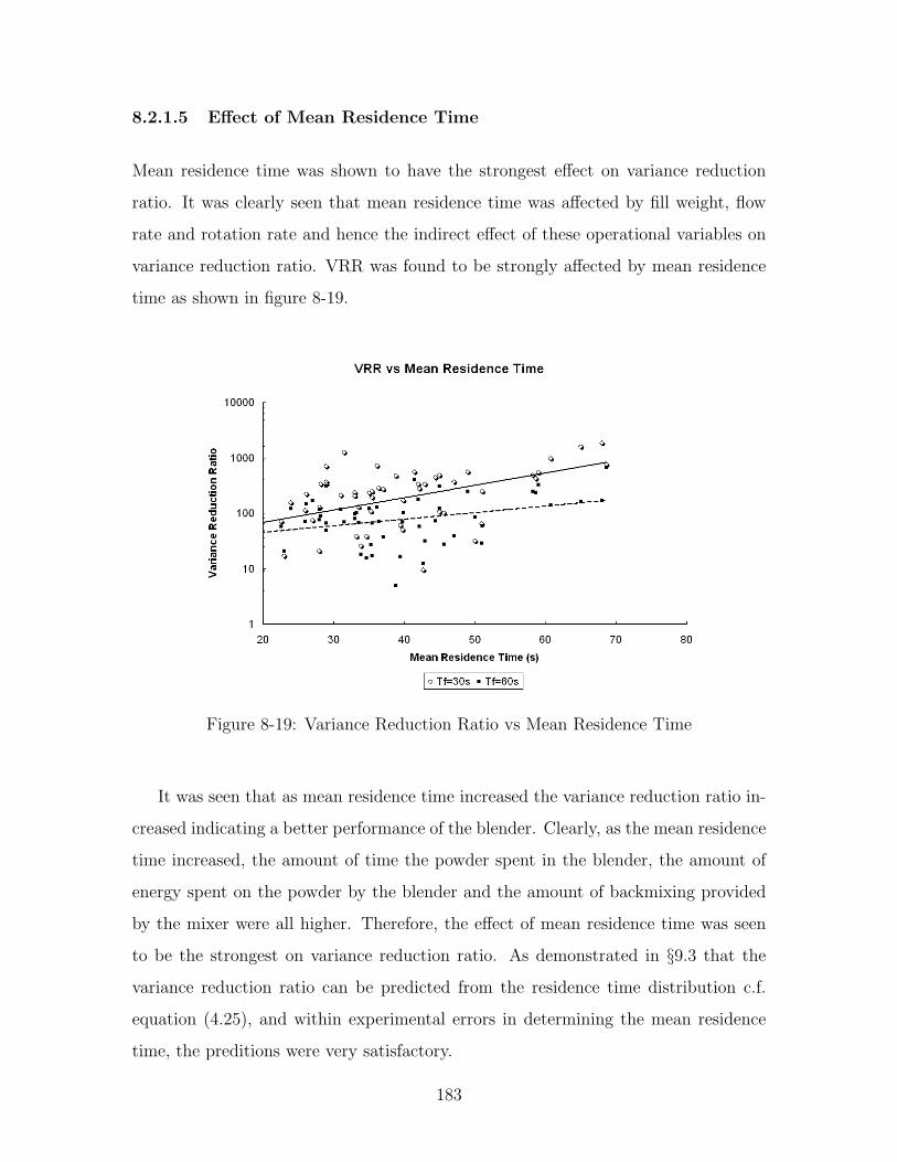
8.2.1.5 Effect of Mean Residence Time
Mean residence time was shown to have the strongest effect on variance reduction
ratio. It was clearly seen that mean residence time was affected by fill weight, flow
rate and rotation rate and hence the indirect effect of these operational variables on
variance reduction ratio. VRR was found to be strongly affected by mean residence
time as shown in figure 8-19.
Figure 8-19: Variance Reduction Ratio vs Mean Residence Time
It was seen that as mean residence time increased the variance reduction ratio in-
creased indicating a better performance of the blender. Clearly, as the mean residence
time increased, the amount of time the powder spent in the blender, the amount of
energy spent on the powder by the blender and the amount of backmixing provided
by the mixer were all higher. Therefore, the effect of mean residence time was seen
to be the strongest on variance reduction ratio. As demonstrated in §9.3 that the
variance reduction ratio can be predicted from the residence time distribution c.f.
equation (4.25), and within experimental errors in determining the mean residence
time, the preditions were very satisfactory.
183

8.2.1.6 Effect of Disturance Time Period
The effect of time period of the fluctuations introduced into the blender on variance
reduction ratio was expected to be in agreement with equation (4.21) where the
variance reduction ratio was proportional to the ratio of mean residence time to time
period of fluctuation entering the blender. It was found that the variance reduction
decreased with increasing fluctuation time period in line with the effect that as the
time period of fluctuation entering the blender increased, the blender was unable
to reduce and modulate the disturbances leading to increased VRRs. It was also
found that the VRR decreased with increasing ratios of mean residence time to time
period of fluctuations entering the blender as shown in figure 8-20. The theoretical
predictions of VRR and dependence on Tm
Tfwill be discussed in §9.3.
Figure 8-20: VRR vs Tm
Tf
8.2.2 Three Component Blending
Three component experimental data and offline samples were collected and analyzed
as described in §7.2 and §7.2.3. The spectral RSD computed from principal compo-
nents of the blending spectra were used to understand the effect of three component
blending as described in §7.2.3. In order to understand the difference between two
184

and three component blending, spectral RSD from the two component blending spec-
tra of experimental runs corresponding to the three component blending experiments
were also computed.
8.2.2.1 Effect of MgSt on API RSD
MgSt was found to have deteriorating effect on the spectral RSDs of caffeine and
acetaminophen. The spectral RSD of caffeine was found to increase when caffeine
was blended with MgSt and lactose DCL-11 as shown in figure 8-21. However, it was
noted that the increase in the spectral RSDs of caffeine upon addition of MgSt was
not very significant at both 4.32 and 8.64 kg/hr.
Figure 8-21: Effect of MgSt on Caffeine RSD in Ribbon Blender
The spectral RSD of acetaminophen was also found to increase when acetaminophen
was blended with lactose DCL-11 and MgSt, as shown in figure 8-22. The increase in
RSD of acetaminophen when MgSt was added was very significant at both 4.32 and
8.64 kg/hr. MgSt decreases the cohesion between particles by means of forming a
thin layer (coat) of MgSt particles around the API and excipient particles. MgSt was
found to have the strongest effect on Acetaminophen because cohesion between ac-
etaminophen particles were brought down from a value of 0.65 to a low of 0.22 mJ/m2
185

compared to a drop from 0.43 to 0.22 mJ/m2 for caffeine. This decrease caused con-
siderable demixing along the length of the blender and therefore resulted in increased
spectral RSDs for acetaminophen.
Figure 8-22: Effect of MgSt on Acetaminophen RSD in Ribbon Blender
8.2.2.2 Effect of Residence Time on API RSD and MgSt RSD
As flow rate increased, the residence time at a given rotation rate of the shaft de-
creased. Hence, from figures 8-21 and 8-22 we found that an decrease in the residence
time increased the spectral RSD of caffeine and acetaminophen. The presence of
MgSt exacerbated the increase in acetaminophen RSD because of reasons already
discussed.
The spectral RSD of magnesium stearate decreased, as shown in figure 8-23, when
blended with acetaminophen, with a decrease in mean residence time (i.e., increase
in flow rate). This decrease in spectral RSD of MgSt implied a well-distributed
MgSt coating on acetaminophen than that of caffeine. Therefore, the RSDs of ac-
etaminophen increased more than that of caffeine due to the addition of MgSt.
186

Figure 8-23: Effect of MgSt on MgSt RSD in Ribbon Blender
8.3 Summary of Results
It was shown that since powders were comprised of discrete particles, the achievement
of steady state and the measurement of fill weights needed averaging over a maximum
and minimum observed fill weights at steady state. Nevertheless, the averaged fill
weights were linearly proportional to flow rate and inversely proportional to rotation
rate. The mean residence times decreased with increasing the shaft rotation rates.
The dependence of dispersion coefficients on operational variables was found to be
inconclusive. There was no apparent trend that was consistent with the physics
of the process and it was expected that it could be a paramater dependent on the
fundamental particle properties than the macroscopic operational variables.
It was shown that the variance reduction ratio was a strong function of mean
residence time and fluctuation time period and was found to be proportional to the
ratio of Tm to Tf . Within the experimenal design space, the axial dispersion coef-
ficient was found not to have a significant effect on variance reduction ratio. The
operational variables like flow rate, shaft rotation rate and fill weight were affecting
the variance reduction ratio only through mean residence time. The effect of three
187

component blending showed that the spread of the third component, lubricant in this
case, dictated the homogeneity of the API. An increase in lubricant deteriorated the
mixture quality.
188
Chapter 9
The Effect of Microscale Propertieson Macroscopic Phenomena
Much like the pheomenological behavior of fluids that depends on the molecular
properties of materials, the phenomenological behavior of powders depends on the
microscopic properties of particles composing the bulk powder. The deteremination
of this relationship is of critical importance in assuring that powder processing phe-
nomena are well understood, well characterized and well controlled. Domike [25] and
Ngain [71] related the microscopic properties of particles like particle size, cohesive
and adhesive surface energies to macroscopically observed phenomena. The effect of
particle size, cohesion and adhesion surface energies and particle shape were examined
in this work and the results are described in subsequent sections.
9.1 Effect of Particle Size
In order to understand the effect of microscopic properties on continuous blender
performance, two sets of experiments were performed. First, the particle size of the
excipient was within the same type of the excipient. Lactose DCL 14 was sieved and
was divided into excipients of two different particle size cuts 45 ≤ D ≤ 150µm
and 150 ≤ D ≤ 250µm. Impulse response experiments (described in §7.1) were
carried out with these excipients and caffeine of a fixed particle size distribution,
Dmean = 200µm and σ = 100µm. The impulse response experimental data were
converted to concentrations and subsequently regressed with the dispersion model c.f.
189

equation (4.9) as described in §7.1.3.
9.1.1 Effect of Size on Bodenstein Number
An increase in size of the excipient particles that forms the bulk of the powder mixture
resulted in a decrease in the Bodenstein number as shown in figure 9-1 at 0◦ incline.
This meant that as particle size of the excipient increased or the size ratio of excipient
to active ingredient increased, the dispersive mixing component in the Bodenstein
number increased in relation to the convective mixing component.
Figure 9-1: Effect of Particle Size on Bodenstein Number
It was expected that as particle size increased, the dispersive component of mix-
ing would be increased as larger particles were expected to overcome the forces of
cohesion and adhesion due to gravity and were expected to disperse more freely in
the mixture. However, A separate evaluation of the dispersive mixing component was
also performed as described below.
9.1.2 Effect of Size on Dispersion Coefficient
As the size of the excipient increased (or the ratio of the excipient to API particle
size increased), the dispersion coefficient increased as shown in figure 9-2. Clearly,
190

particle size played a critical role in determining the extent of dispersive mixing in
the blender. As particle size increased, Ngai [71] showed that the particle balanced
the forces of gravity with cohesive and adhesive forces. If the size was increased
even further, the cohesive effect of the particles no longer played a role in holding
the particles together and hence random movement of particles on the free surface
generated by the movement of the ribbons in the blender increased. This increased
random movement resulted in increased dispersion coefficients as shown in figure 9-2.
Figure 9-2: Effect of Particle Size on Dispersion Coefficient
9.1.3 Effect of Size on Variance Reduction Ratio
The effect of increasing the particle size of excipient at constant API particle size on
blender performance was theoretically estimated. The theoretical estimation proce-
dure was carried out on the basis of equation (4.16). The variance reduction ratio was
determined by using the experimentally determined RTD and the sinusoidal forcing
input function of equation (4.18). Two disturbance time periods, 30 and 50 seconds,
were used in determining the theroretical variance reduction ratios for the RTDs from
the two different particle size distributions (whose dispersion coefficients were shown
191

in figure 9-2).
As the particle size increased, the variance reduction ratio plotted as a function of
the mean residence time was higher for the particles of larger excipient size. This was
observed at both the disturbance time periods as shown in figures 9-3 and 9-4. The
effect of time period of fluctuation was also seen to be in consonance with observations
made before on the effect blender performance due to the time period of fluctuation.
As seen in figures 9-5 and 9-6, the variance reduction ratio decreased with in-
creasing time periof of the input fluctuations, indicating that as the time period of
fluctuations increased, the blender was unable to modulate or reduce the variance
at the inlet. This was in consonance with the observation made from literature, as
shown in equation (4.21) and from the results of blending experiments at two distinct
input fluctuation time periods as described in §7 and figure 8-20.
Figure 9-3: Effect of Particle Size on VRR Tf = 30s
9.2 Effect of Microscale Properties
The effect of microscale properties like cohesive and adhesive surface energy, effect
of shape of particle and the effect of lubricant were studied by varying the types
192

Figure 9-4: Effect of Particle Size on VRR Tf = 50s
Figure 9-5: Effect of Time Period of Fluctuation on Theoretical VRR, 45 ≤ D ≤150µm
193
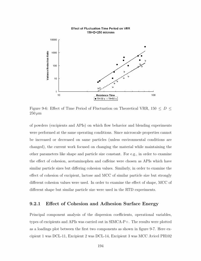
Figure 9-6: Effect of Time Period of Fluctuation on Theoretical VRR, 150 ≤ D ≤250µm
of powders (excipients and APIs) on which flow behavior and blending experiments
were performed at the same operating conditions. Since microscale properties cannot
be increased or decreased on same particles (unless environmental conditions are
changed), the current work focused on changing the material while maintaining the
other parameters like shape and particle size constant. For e.g., in order to examine
the effect of cohesion, acetaminophen and caffeine were chosen as APIs which have
similar particle sizes but differing cohesion values. Similarly, in order to examine the
effect of cohesion of excipient, lactose and MCC of similar particle size but strongly
different cohesion values were used. In order to examine the effect of shape, MCC of
different shape but similar particle size were used in the RTD experiments.
9.2.1 Effect of Cohesion and Adhesion Surface Energy
Principal component analysis of the dispersion coefficients, operational variables,
types of excipients and APIs was carried out in SIMCA-P+. The results were plotted
as a loadings plot between the first two components as shown in figure 9-7. Here ex-
cipient 1 was DCL-11, Excipient 2 was DCL-14, Excipient 3 was MCC Avicel PH102
194

and Excipient 4 was MCC Celphere CP-102. Active ingredient 1 was caffeine and 2
was acetaminophen.
All correlations were found by taking the scalar product of the position vectors
of the observed response in the loadings plot with the parameter of interest. For
example, acetaminophen (Act(2)) was found to negatively correlate with dispersion
coefficient while caffeine (Act(1)) was foung to positively correlate with dispersion
coefficient in figure 9-7. Caffeine’s cohesion energy was lesser than the cohesion en-
ergy of acetaminophen from table 4.3. As cohesion energy increases, the dispersion
coefficient decreases. Thus, this explained the reason why going from acetaminophen
to caffeine the dispersion coefficients increased.
Figure 9-7: Loadings Plot of Effect of Excipients and APIs
Similarly, excipient 2, DCL-14 was found to have a strong correlation with dis-
persion coefficient when compared with excipient 1, DCL-11. This was attributed to
the excipient to active ingredient particle size ratio. DCL-14 comprised of larger par-
ticles that gave rise to increased dispersion coefficients. Excipients 3 and 4 were both
MCC particles which had high cohesion values. As a result of high cohesion, these
excipients correlated negatively with dispersion coefficients and had approximately
195

equal scalar products. Clearly, increasing cohesion energy and dispersion coefficients
showed a negative correlation over all the materials observed. The dispersive nature
of particles therefore was strongly dependent on the microscopic surface energies of
the particle.
Changing the active ingredients, caffeine to acetaminophen, did not affect the
mean residence time since the line from API 1 to API 2 is orthogonal to mean res-
idence time, indicating a zero scalar product. Since the bulk of the powder flowing
in the blender was the excipient, it was expected that the excipient properties would
dominate the dependence of mean residence time. In going from lactose to cellulose,
where the cohesion energies were higher for cellulose, it was found to reduce the mean
residence time. However, it was noted that the bulk density of the cellulose Avicel
PH102 (excipient 3) was much lower than that of lactose which caused the powder
to exit out of the system in a shorter time.
9.2.2 Effect of Particle Shape
As the particle shape was changed by changing the excipient from needle and flat
plate MCC Avicel PH-102 particle to spherical Celphere CP-102 particles, the dis-
persion coefficient remained the same as shown in figure 9-7. However, it was found
that the mean residence time was positively correlated with spherical Celphere MCC
particles. It was found that the fill weight of the blender positively correlated with
MCC Celphere CP-102 as the density of CP-102 was much higher than density of
MCC Avicel PH-102. It was expected that a change in shape caused changes in den-
sity and increased the fill volume in the blender for the same fill weight and caused
the activated the second window at the exit. As a result, the residence times of the
particles were observed to be less for MCC Avicel PH-102 when compared with MCC
Celphere CP-102.
9.2.3 Effect of Lubricant
Magnesium stearate was shown to influence the blending process by coating the ex-
cipient and API particles with a fine layer of lubricant particles. The interaction of
196
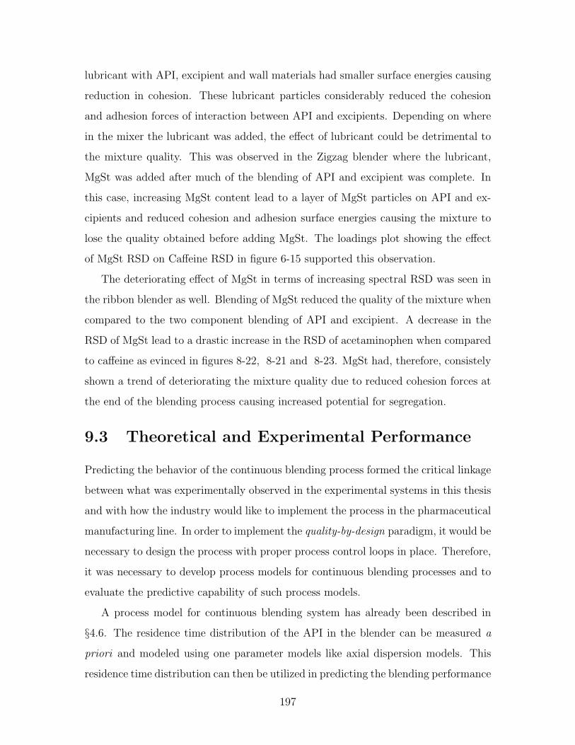
lubricant with API, excipient and wall materials had smaller surface energies causing
reduction in cohesion. These lubricant particles considerably reduced the cohesion
and adhesion forces of interaction between API and excipients. Depending on where
in the mixer the lubricant was added, the effect of lubricant could be detrimental to
the mixture quality. This was observed in the Zigzag blender where the lubricant,
MgSt was added after much of the blending of API and excipient was complete. In
this case, increasing MgSt content lead to a layer of MgSt particles on API and ex-
cipients and reduced cohesion and adhesion surface energies causing the mixture to
lose the quality obtained before adding MgSt. The loadings plot showing the effect
of MgSt RSD on Caffeine RSD in figure 6-15 supported this observation.
The deteriorating effect of MgSt in terms of increasing spectral RSD was seen in
the ribbon blender as well. Blending of MgSt reduced the quality of the mixture when
compared to the two component blending of API and excipient. A decrease in the
RSD of MgSt lead to a drastic increase in the RSD of acetaminophen when compared
to caffeine as evinced in figures 8-22, 8-21 and 8-23. MgSt had, therefore, consistely
shown a trend of deteriorating the mixture quality due to reduced cohesion forces at
the end of the blending process causing increased potential for segregation.
9.3 Theoretical and Experimental Performance
Predicting the behavior of the continuous blending process formed the critical linkage
between what was experimentally observed in the experimental systems in this thesis
and with how the industry would like to implement the process in the pharmaceutical
manufacturing line. In order to implement the quality-by-design paradigm, it would be
necessary to design the process with proper process control loops in place. Therefore,
it was necessary to develop process models for continuous blending processes and to
evaluate the predictive capability of such process models.
A process model for continuous blending system has already been described in
§4.6. The residence time distribution of the API in the blender can be measured a
priori and modeled using one parameter models like axial dispersion models. This
residence time distribution can then be utilized in predicting the blending performance
197

as described in §4.6 using equations (4.16) for determining the theoretical VRR and
(4.25) for determining the prediction intervals arising due to errors in mean residence
time.
9.3.1 Prediction of VRR from Axial Disperision RTD Model
Online process control of a continuous manufacturing process was mentioned as one
of the main advantages of shifting from batch to continuous mode of processing. In
order to implement process control, process models must be developed for designing
controllers. In chapter 8, the axial dispersion model was shown to depict the flow
behavior of the blender well. It was also discussed in §4.6, that the RTD model can be
used to predict VRR using equation (4.25). In this section, experimentally measured
RTD data were used in predicting the variance reduction ratio and effect of errors in
mean residence time were discussed.
Figure 9-8: Non-linear Regression of Axial Dispersion Model with NIR Data
When model parameters obtained from non-linear regression of experimental RTD
data with the axial dispersion model were used, the predicted VRR’s were 3− 4 orders
of magnitude higher than the experimentally observed values as depicted in figure 9-9.
This meant that the axial dispersion model overpredicted the blender performance to
a very large extent. From the statistical regression of the experimental data to axial
dispersion model shown in figure 9-8,it was suspected that the deviation from the
198

axial dispersion model was causing this over-prediction. In other words, statistical
regression of RTD data was suspected to smoothen the natural variance in the RTD
data.
Figure 9-9: Over-prediction of Variance Reduction Ratio
This hypothesis was tested, by predicting the blending profiles by first using the
axial dispersion model and then using an axial dispersion model with an addition of
magnitude dependent gaussian noise. The smoothened and noise-added RTD’s are
shown in figure 9-10. A magnitude dependent gaussian noise that was 20% of the
magnitude of the dispersion model was added as shown in the figure 9-10.
The predicted blending profiles before and after the axial dispersion model was
mixed with the aforementioned noise was shown in figures 9-11 and 9-12 respectively.
By mixing the axial dispersion model with the magnitude dependent Gaussian noise,
it was observed that the variance reduction ratios fell by 103 − 104, increasing the
possibility of matching with the experimentally observed VRRs.
This analysis showed the importance of two attributes of powder mixtures that
demand further investigation. The first attribute was the fact that use of the axial
dispersion model was smoothing and eliminating inherent variance existing in the
powder mixture. This noise arose from the chaotic behavior of powder in the blender
199

Figure 9-10: Axial Dispersion RTD with Magnitude Dependent Gaussian Noise
and due to distributions in micro-scale properties like size, shape, cohesion, adhesion
and friction. Thus, in order to improve the predictions of variance reduction ratio, it
was necessary to use data that reflected the noise and variance present in the blender.
As a result, experimentally measured residence time distributions were used as the
RTD models instead of the axial dispersion model.
The second attribute was that the scale of scrutiny of the powder mixture, as
discussed in chapter 2, should depend on the scale of segregation. Powders being
inherently discrete materials, require to be sampled at a certain scale of scrutiny to
determine the quality of the mixture. But the online non-invasive measurements on
the ribbon blender were performed at very high frequencies over very small scales
of scrutiny of the powder mixture. This was remedied by a moving average model
described after the theoretical predictions of VRR.
200
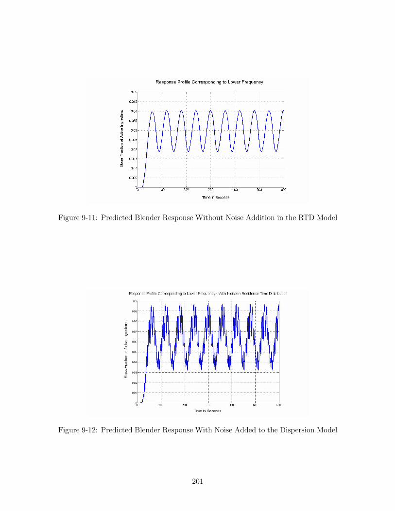
Figure 9-11: Predicted Blender Response Without Noise Addition in the RTD Model
Figure 9-12: Predicted Blender Response With Noise Added to the Dispersion Model
201
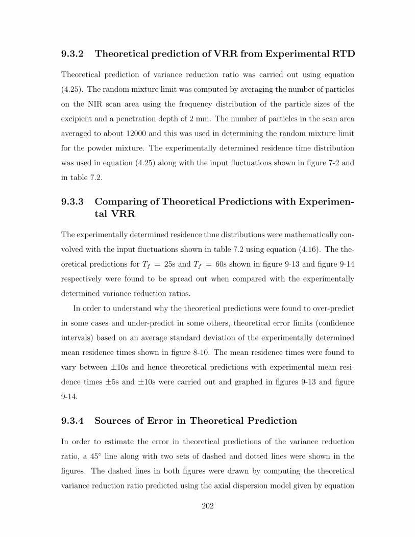
9.3.2 Theoretical prediction of VRR from Experimental RTD
Theoretical prediction of variance reduction ratio was carried out using equation
(4.25). The random mixture limit was computed by averaging the number of particles
on the NIR scan area using the frequency distribution of the particle sizes of the
excipient and a penetration depth of 2 mm. The number of particles in the scan area
averaged to about 12000 and this was used in determining the random mixture limit
for the powder mixture. The experimentally determined residence time distribution
was used in equation (4.25) along with the input fluctuations shown in figure 7-2 and
in table 7.2.
9.3.3 Comparing of Theoretical Predictions with Experimen-tal VRR
The experimentally determined residence time distributions were mathematically con-
volved with the input fluctuations shown in table 7.2 using equation (4.16). The the-
oretical predictions for Tf = 25s and Tf = 60s shown in figure 9-13 and figure 9-14
respectively were found to be spread out when compared with the experimentally
determined variance reduction ratios.
In order to understand why the theoretical predictions were found to over-predict
in some cases and under-predict in some others, theoretical error limits (confidence
intervals) based on an average standard deviation of the experimentally determined
mean residence times shown in figure 8-10. The mean residence times were found to
vary between ±10s and hence theoretical predictions with experimental mean resi-
dence times ±5s and ±10s were carried out and graphed in figures 9-13 and figure
9-14.
9.3.4 Sources of Error in Theoretical Prediction
In order to estimate the error in theoretical predictions of the variance reduction
ratio, a 45◦ line along with two sets of dashed and dotted lines were shown in the
figures. The dashed lines in both figures were drawn by computing the theoretical
variance reduction ratio predicted using the axial dispersion model given by equation
202
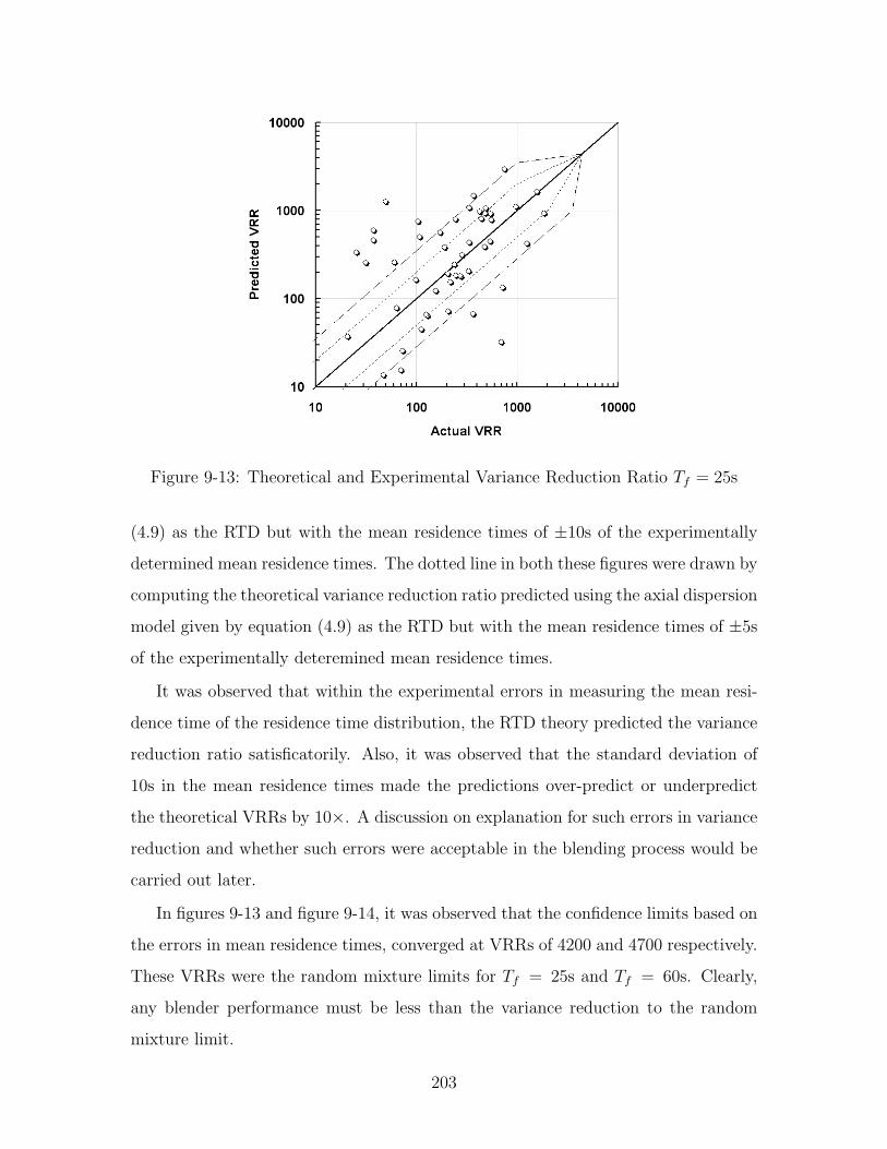
Figure 9-13: Theoretical and Experimental Variance Reduction Ratio Tf = 25s
(4.9) as the RTD but with the mean residence times of ±10s of the experimentally
determined mean residence times. The dotted line in both these figures were drawn by
computing the theoretical variance reduction ratio predicted using the axial dispersion
model given by equation (4.9) as the RTD but with the mean residence times of ±5s
of the experimentally deteremined mean residence times.
It was observed that within the experimental errors in measuring the mean resi-
dence time of the residence time distribution, the RTD theory predicted the variance
reduction ratio satisficatorily. Also, it was observed that the standard deviation of
10s in the mean residence times made the predictions over-predict or underpredict
the theoretical VRRs by 10×. A discussion on explanation for such errors in variance
reduction and whether such errors were acceptable in the blending process would be
carried out later.
In figures 9-13 and figure 9-14, it was observed that the confidence limits based on
the errors in mean residence times, converged at VRRs of 4200 and 4700 respectively.
These VRRs were the random mixture limits for Tf = 25s and Tf = 60s. Clearly,
any blender performance must be less than the variance reduction to the random
mixture limit.
203

Figure 9-14: Theoretical and Experimental Variance Reduction Ratio Tf = 60s
9.4 Effect of Scale of Scrutiny
Just as the smallest element that influences properties of and phenomena in a fluid is
a molecule, the smallest element that has significance in properties and phenomena
in powders is a particle. At the particle level, the powder mixture is completely seg-
regated, since each particle is comprised of a chemically unique species. As discussed
in the chapter 2, the scale of segregation depends on the scale of scrutiny at which
we are investigating the properties of the powder mixture.
As the scale of scrutiny decreases, the scale of segregation decreases. In other
words, if we examine the entire powder mixture, the mixture would seem to be com-
pletely mixed. However, as we divide the mixture into parts, we find that the indi-
vidual parts would be different in composition and that there would be a variance
between each of these parts. If we make these divisions all the way to the particle
level, we find that the variance between the parts (in this case individual particles) to
be the highest. Therefore, it is important to understand and decide a relevant scale
of scrutiny for examination of the powder mixture.
In the case of pharmaceutical powder mixtures, the FDA had mandated that the
204
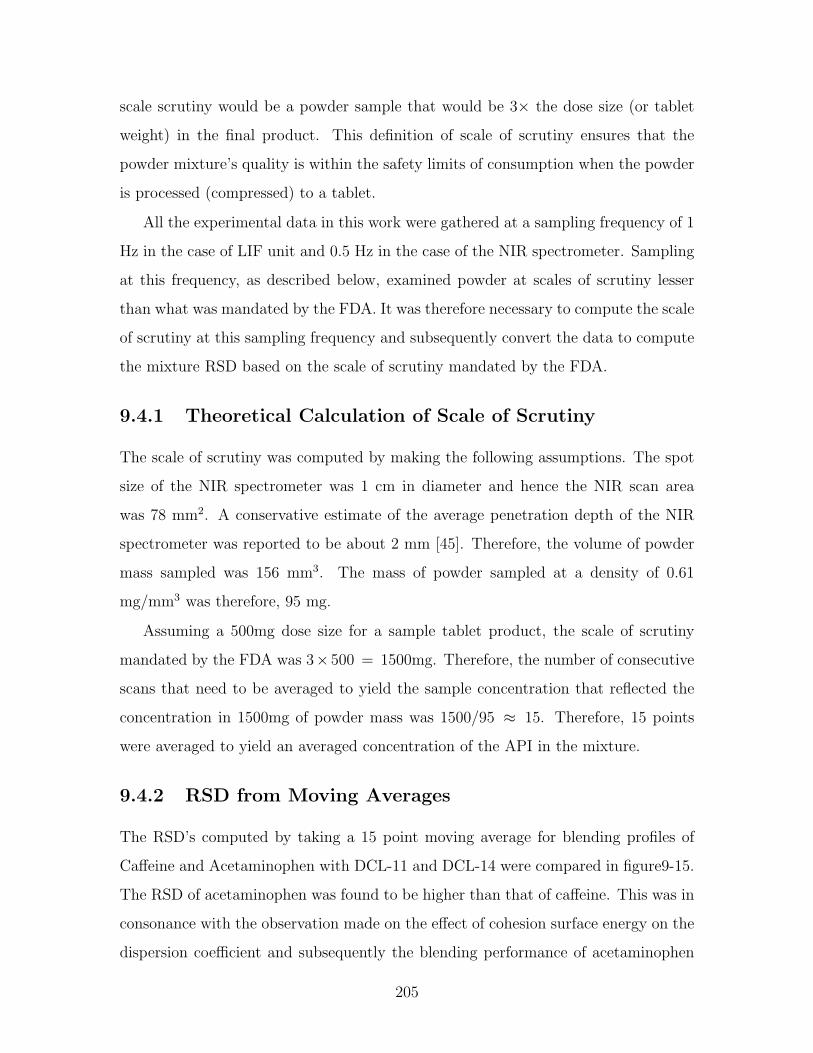
scale scrutiny would be a powder sample that would be 3× the dose size (or tablet
weight) in the final product. This definition of scale of scrutiny ensures that the
powder mixture’s quality is within the safety limits of consumption when the powder
is processed (compressed) to a tablet.
All the experimental data in this work were gathered at a sampling frequency of 1
Hz in the case of LIF unit and 0.5 Hz in the case of the NIR spectrometer. Sampling
at this frequency, as described below, examined powder at scales of scrutiny lesser
than what was mandated by the FDA. It was therefore necessary to compute the scale
of scrutiny at this sampling frequency and subsequently convert the data to compute
the mixture RSD based on the scale of scrutiny mandated by the FDA.
9.4.1 Theoretical Calculation of Scale of Scrutiny
The scale of scrutiny was computed by making the following assumptions. The spot
size of the NIR spectrometer was 1 cm in diameter and hence the NIR scan area
was 78 mm2. A conservative estimate of the average penetration depth of the NIR
spectrometer was reported to be about 2 mm [45]. Therefore, the volume of powder
mass sampled was 156 mm3. The mass of powder sampled at a density of 0.61
mg/mm3 was therefore, 95 mg.
Assuming a 500mg dose size for a sample tablet product, the scale of scrutiny
mandated by the FDA was 3×500 = 1500mg. Therefore, the number of consecutive
scans that need to be averaged to yield the sample concentration that reflected the
concentration in 1500mg of powder mass was 1500/95 ≈ 15. Therefore, 15 points
were averaged to yield an averaged concentration of the API in the mixture.
9.4.2 RSD from Moving Averages
The RSD’s computed by taking a 15 point moving average for blending profiles of
Caffeine and Acetaminophen with DCL-11 and DCL-14 were compared in figure9-15.
The RSD of acetaminophen was found to be higher than that of caffeine. This was in
consonance with the observation made on the effect of cohesion surface energy on the
dispersion coefficient and subsequently the blending performance of acetaminophen
205

Figure 9-15: RSD from Moving Average Model
compared with caffeine. Caffeine was less cohesive compared with acetaminophen and
the RSDs achieved when caffeine was used as the API were higher than the RSDs
achieved when acetaminophen was used as the API.
As mentioned in the section §7.2, powder samples were collected in glass vials at
the end of ribbon blender during some of the experiments. The collected samples
were placed on the NIR spectrometer and offline spectra were collected. These offline
spectra were converted to concentrations using the PLS calibration models shown in
table 4.2. The results from the offline sample collection and spectral analysis were
compared with the results from the 15 point moving average profiles.
The variance reduction ratios computed using these two methods shown in figure
9-16 was found to be in fair agreement with each other (considering the fact that the
variance in VRR within blending experiments was very large as evinced by figures
8-20, 9-13 and 9-14. Therefore, It was found that performing a moving average com-
putation of the blending profiles smoothed the data and matched the online observed
API concentrations with the concentrations of the offline samples.
206

Figure 9-16: Compariosn of VRR from Offline Sample Spectra and Moving Averageof Online Data for MCC Avicel
207

208

Chapter 10
Path for Future Research
Continuous dry powder blending is the starting point in a larger roadmap for trans-
forming the current manufacturing paradigm in pharmaceuticals to one that involves
continuous assessment and improvement. While the current thesis work focused on
dissecting the phenomenological behavior of pharmaceutical powder blending into
powder flow behavior and blender performance modeling and assessment, the lessons
learnt from this work will be widely applicable to other unit operations that are
potential candidates for moving from a batch mode to continuous mode of operation.
The suggested path for future research will be divided into three sections. First,
the path for future research in continuous blending of pharmaceutical powders will
be discussed. Following this, an assessment of the potential for the other unit oper-
ations in seconday pharmaceutical manufacturing to move to a continuous mode of
operation will be discussed. And, finally, a systems analysis of continuous secondary
manufacturing in pharmaceuticals will be needed to be carried out.
10.1 Path for Continuous Blending Research
The current thesis focused on one blender type in high-shear and one blender type
in moderate shear blenders. The material choices were driven by needs felt by the
industrials sponsors of the research work, in addition to prior experience in classifying
and characterizing the microscopic properties of these powders. The variables chosen
in this work were a result of both what the literature suggested to be worthwhile in
examining as well as a physical understanding of the phenomenological behavior of
209
particles in powder mixtures. However, there are many promising avenues pursuing
which might prove to be very rewarding both academically and in practice in the
industry. These avenues are discussed below.
10.1.1 Blender Design
As mentioned earlier, the choice and design of the experimental blending shrank the
experimental design space by the largest fraction. Therefore, examining different
blender types and mechanisms for mixing powders in them will be useful not only
in characterizing and benchmarking that blender type but also in understanding the
limits of the design space defined by the types, characteristics and specificationss of
materials and changeable operational and environmental parameters to be used in
process.
One of the early design decisions made in this work was to work with small quan-
tities of powder in the order of 1 − 10 kg/hr. The laboratory scale helical ribbon
blender was designed to mix powder at the current industrial production rate of
100,000 tph (tablets per hour). The decision to keep the blender size small was spec-
ulated to be one of the causes behind the wide variation in results, most importantly,
the theoretical and experimental predictions using the theories described in this work.
Thus, one of the future research goals in using double helical ribbon blender would
be to increase the volume and residence times of the powder in the blender which are
expected to reduce the variations observed in the blending process. It is envisioned
that the ribbon blender designed in this work would be appended with an extension
piece that would increase the length, volume and residence times of the the powder
in the mixture.
In addition to increasing residence times and fill weights of the powder in the
blender, recycle of powder from the exit to the entrance will also cause additional
mixing (increased back-mixing) and would approach the desired ideal blending be-
havior. Also, this recycle arrangement would extend the lower limit of API content as
two staged mixing can be carried out in such a recycle based ribbon blender. Thus,
one of the future research goals should be experimentally design and test such a
210

recycle system for powder mixing.
Literature review revealed that high shear powder blenders, like zigzag blenders,
delivered better blend performance due to the combined effects of shear, convective
and dispersive mixing and by imparting higher energies into powders. Moderate
shear mixers, like the ribbon blender, impart less energy than high shear mixers,
but work considerably well for most cohesive powders. Therefore, a change in the
internal shaft design to simple systems to incorporate newer designs like paddled,
paddled with ribbons etc., will increase the dispersion coefficient and back mixing of
the material in the blender. These changes in design of the internal blending elements
are seen as one of the future potential research directions for the work on continuous
dry powder blending.
10.1.2 Material Properties
A number of raw material properties were examined in this work. Particle size,
cohesion and adhesion and shape of particles were examined in great detail. Much
of this work was done by changing the excipients and APIs while trying to maintain
the other properties constant within reasonable experimental errors. This method of
experimentally examining the effects of microscopic properties has both merits and
demerits.
The materials used in the experiments in this work reflected the choice of excipients
and APIs with properties that mirror those available for the pharmaceutical industry.
In this sense, the work reflected the material choices faced by formulation scientists
in pharmaceutical industry and hence examined the effect of varying microscopic
properties withing these constraints of commercially available materials. However,
there is a critical need to examine the effect of varying the microscopic properties of
materials independently. This can be achieved both by experiment and simulation.
In experiment, the material properties can be modified by pre-treatment. There
are many choices for pre-treatment: solvent treatment, milling, granulation are a
few examples. However, the effect of pre-treatment will have to be characterized
before blending experiments on pre-treated materials is accomplished. Alternatively,
211

a simulation based approach would be very effective in determining the effect of
varying microscopic properties independently.
Discrete Element Method simulations, discussed in the literature review, mathe-
matically solve the kinematics and dynamics equations of particle movement in the
powder bed. These simulation techniques were used by Domike [25] and Ngai[71]
in understanding the effect of microscopic properties on macroscopic phenomena.
These multiscale analytical techniques can be employed in understanding the effect
of altering the microscopic properties like particle size, cohesion/adhesion, shape and
friction on blending by use of DEM simulations. However, DEM simulations need
long computational times for statistically valid results to be generated. Therefore, an
intermediate mesoscale modeling of the blending operation, like residence time dis-
tribution models or markov chain models could be employed to predict the blending
performance.
10.1.3 Environmental Variables
Environmental variables like humidity and temperature play a very critical role in
pharmaceutical processes. Humidity changes the moisture content of powders and
increases the cohesive forces by forming liquid bridges between particles. Tempera-
ture, can affect these liquid bridges via it’s effect on surface tension and can increase
or decrease the cohesive effect.
It was decided in the beginning not to examine the effect of controlling these en-
vironmental variables in this work. However, the final implementation of continuous
pharmaceutical processes will have to consider the effect of environmental variables.
Therefore, examining the effect of humidity on the blending process will be a neces-
sary step before implementation of continuous blending operation in pharmaceutical
secondary manufacturing.
10.1.4 Analytical Techniques
In this work, non-invasive analytical techniques like LIF and NIR spectroscopy were
employed to assess the quality of the powder mixture and the state of the blending
212

process. The measurement was carried out at the wall of the blending process and
was found to correlate fairly accurately with the bulk of the powder based on our
observations on offline and online sample analysis. However, the need for advances
in analytical techniques that can probe the bulk of the powder mixture for structure
and segregation.
Capacitive probes [86] have the potential to examine the powder bulk, but lacked
the capability to differentiate between the chemical identities and chemometric prop-
erties of APIs and excipients. It would be worthwhile to develop new analytical
techniques based on the capacitive probe principle but using spectroscopy as the
basis for differentiating the chemometric properties.
Another alternative would be to develop at-line analytical techniques like drawing
off a portion of the material from the exit for automated LIF/NIR spectral analysis
and subsequently returning the sample stream to the bulk would reflect the powder
mixtures structure better than surface measurements.
10.2 Transforming Batch to Continuous
In the introduction, it was discussed that blending was the last unit operation where
variance was introduced before the powder was finalized into the final product form,
the tablet of capsule. It was also discussed that the unit operations preceeding blend-
ing were all currently batch processes and succeeding blending were quasi-continuous
operations (operations that are inherently continuous, but being run in a batch mode
as the whole process is operated in batches).
The next step in implementing continuous manufacturing in secondary pharma-
ceutical manufacturing would be examine the transformation of these operations pre-
ceeding blending operations. As the current manufacturing processes in the pharma-
ceutical industry are all batch processes, transformation to continuous operation must
need to progress in steps. The process of implementing continuous operations will
involve a considerable amount of research effort in not only developing process un-
derstanging of each individual operations, but also a systems view of what is the best
path to implementation, in what order should the unit operations be transformed to
213

continuous mode and whether a complete rethinking and redesign of pharmaceutical
operations would be justified for improving the efficiency in manufacturing.
10.2.1 Crystallization
Continuous crystallization is a new area of research in pharmaceutical manufacturing
and is being currently investigated. Control of kinetic rates of formation of crys-
tals, the size distribution and crystal faces determine the properties of the API that
will be used in the subsequent operations. The effect of thermodynamic and kinetic
properties of mother liquors and crystals will be required for understanding and im-
plementing continuous crystallization process.
10.2.2 Granulation
Continuous granulation devices are being employed in food and construction indus-
tries. The challenges in continuous granulation are around prediction of particle size
growth, mechanical and surface properties of particles formed and understanding the
evolution of cohesion, adhesion and surface frictional energies on particles during
granulation. It is worthwhile to note that granulation is generally employed as a
corrective operation of changing particle size, shape and morphology and hence if the
crystallization step and choice of excipients are carried out optimally, milling step
could be avoided.
10.2.3 Drying
Continuous dryers are employed in many process industries where the volumes of
the product are very large. Developing process models to control the quality of the
product coming out of a continuous dryer will require development of reliable process
sensors for measuring the moisture content inside the powder bed. NIR sensors have
been used to determine moisture content, but are not reliable predictors of powder
bed moisture. The theory and design of continuous dryers and effect of particle
properties like particle size have been investigated in other process industries, notably
manufacture of chemical solids like common salt.
214

10.2.4 Milling
Continuous milling operation has been employed in a number of industries. The
challenges in continuous milling are around controlling the particle size distribution
of the product and imparting uniform energy density to particles of different sizes.
Like granulation, milling is generally employed as a corrective operation of changing
particle size, shape and morphology and hence if the crystallization step and choice
of excipients are carried out optimally, milling step could be avoided.
10.3 Economic Analysis of Continuous Blending
The economic argument for implementing continuous processes in general and con-
tinuous blending in particular in a pharmaceutical setting needs to be examined.
Further work on this area should focus on analyzing the economics of continuous pro-
cessing and need provide a framework to assess the business impact of implementing
continuous manufacturing.
215

216

Chapter 11
A Framework for GlobalPharmaceutical ManufacturingStrategy
Worldwide pharmaceutical sales for the top 11 ’big pharma’ were over $270 billion
in 2006. The year on year earnings growth was over 6.5% indicating a strong sector
with considerable potential for value creation in the developed world [89]. Devel-
oping nations like India, China, Russia and Brazil have seen significant increases in
healthcare spending in the past five years. Countries like India and China have also
become favorite destinations for some pharmaceutical companies to establish satellite
distribution locations. Since 1998, pharmaceutical industry has been experiencing
increased pressure to improve bottom-line performance in the face of drug patent
expirations. Drugs like Losec and Prilosec lost patent protection in 1999 and block-
busters like Zocor and Zoloft lost patent protection between 2005 and 2007.
This increased pressure has forced pharmaceutical companies to examine sources
of value along its entire value chain. Research and product development were always
seen as activities that added shareholder value. Pharmaceutical manufacturing was
perceived as a cost center rather than value adding activity along the pharmaceutical
value chain. Reports of manufacturing issues and increasing pressure from generics on
off patent drugs have forced pharmaceutical companies to re-examine their strategies
in manufacturing.
In addition to investing in bringing science into pharmaceutical manufacturing,
217

pharmaceutical companies have focused on an integrated strategy of building value by
expanding manufacturing to countries outside of US, EU and Japan. This capstone
project focuses on the development of the pharmaceutical manufacturing outside of
US, EU and Japan. For the purposes of this discussion, we will consider both phar-
maceutical (small molecule) and biologics (large molecule proteins) manufacturing
together unless otherwise a distinction is made.
11.1 Overview of Manufacturing
Pharmaceutical manufacturing described earlier in this thesis contains two distinct
sequence of steps called primary synthesis (of the API) and secondary manufacturing
(of the drug product) and is shown in figure 11-1. The formulated drug product is then
taken to a fill finish facility where the final product is packaged and labeled according
to the market and regulatory specifications. In biologic manufacturing, the steps
begin with either a fermentation process where genetically modified microorganisms
synthesize API or mammalian synthesis where genetically modified mammalian cells
are carefully grown in bioreactors and the complex protein products are synthesized.
This is then purified in the downstream processing stages and sent to secondary
manufacturing where the drug product is finally formulated as seen in figure 11-
2. Just like in pharmaceutical manufacturing, the last stage involves a fill-finish
process after which the product is packaged according to market needs and regulatory
specifications.
11.1.1 Differences between Pharmaceuticals and Biologics
There are a number of important distinctions between pharmaceutical (small molecule
API) and biologics (large molecule proteins) therapeutics. Small molecule manufac-
turing process is based on chemical synthesis while large molecule proteins are grown
inside genetically modified microorganisms that synthesize the therapeutic. Chemical
syntheses are much easier to replicate and transfer than microbial fermentation based
synthesis.
218

Figure 11-1: Schematic of Pharmaceutical Manufacturing
Figure 11-2: Schematic of Biologics Manufacturing
The technological complexity of biologics manufacturing and significant intellec-
tual property infringement risks and technology transfer risks are some of the chal-
lenges that biologics companies have to overcome in globalization of manufacturing.
A higher average capital outlay in biologics ($400 million compared to $100 million for
pharmaceuticals) also plays a role in determining the level and spread of globalization
of manufacturing.
11.1.2 Pharmaceutical Manufacturing Output
Data from UNIDO industrial statistics database [79] showed that the real pharma-
ceutical manufacturing output has been steadily flattening from 1997 to 2002. While
the real GDP growth has been between 0.8% and 1.5%, the Purchasing Power Parity
(PPP)-adjusted pharmaceutical manufacturing output has risen steadily as seen in
figures 11-3 and 11-4. In order to derive the PPP conversion factor for a particular
country, the ratio of Purchasing Power Parity based GDP to Real GDP was used [2]
and is shown in table 11.1.
219
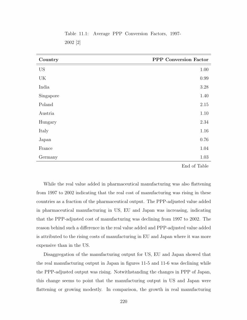
Table 11.1: Average PPP Conversion Factors, 1997-
2002 [2]
Country PPP Conversion Factor
US 1.00
UK 0.99
India 3.28
Singapore 1.40
Poland 2.15
Austria 1.10
Hungary 2.34
Italy 1.16
Japan 0.76
France 1.04
Germany 1.03
End of Table
While the real value added in pharmaceutical manufacturing was also flattening
from 1997 to 2002 indicating that the real cost of manufacturing was rising in these
countries as a fraction of the pharmaceutical output. The PPP-adjusted value added
in pharmaceutical manufacturing in US, EU and Japan was increasing, indicating
that the PPP-adjusted cost of manufacturing was declining from 1997 to 2002. The
reason behind such a difference in the real value added and PPP-adjusted value added
is attributed to the rising costs of manufacturing in EU and Japan where it was more
expensive than in the US.
Disaggregation of the manufacturing output for US, EU and Japan showed that
the real manufacturing output in Japan in figures 11-5 and 11-6 was declining while
the PPP-adjusted output was rising. Notwithstanding the changes in PPP of Japan,
this change seems to point that the manufacturing output in US and Japan were
flattening or growing modestly. In comparison, the growth in real manufacturing
220

Figure 11-3: Pharmaceutical Output and Value Added for OECD Countries
Figure 11-4: PPP-Adjusted Output and Value Added for OECD Countries
221

Figure 11-5: Pharmaceutical Output for US, EU and Japan
output from EU was significant, but on a PPP-adjusted basis EU showed similar
flattening or modest growth just like US and Japan.
11.1.3 Asia and Eastern Europe Manufacturing Output
It is important to observe that while PPP-adjustment brings out the equivalent value
of the pharmaceutical output in a given country on a uniform basis, this conversion
would mean that the pharmaceutical output from that country or region was sold in
the global market without any market frictions. Therefore, PPP-adjustment is a semi-
empirical, uniform valuation of the output and value added of the pharmaceutical
output of a particular country.
A steady growth in Asian manufacturing output was observed from 1997 to 2002
according to the UNIDO INDSTAT data shown in figures. The first observation to
make is that the real manufacturing output seemed to be flattening in India, when
compared to that in Singapore or South Korea as seen in figure 11-7. Even on a
PPP-adjusted basis, the value of the India’s pharmaceutical output, seen in figure
11-8, was growing very modestly when compared to Singapore. Clearly, Singapore
222

Figure 11-6: PPP-Adjusted Output for US, EU and Japan
Figure 11-7: Pharmaceutical Output for Asia
223
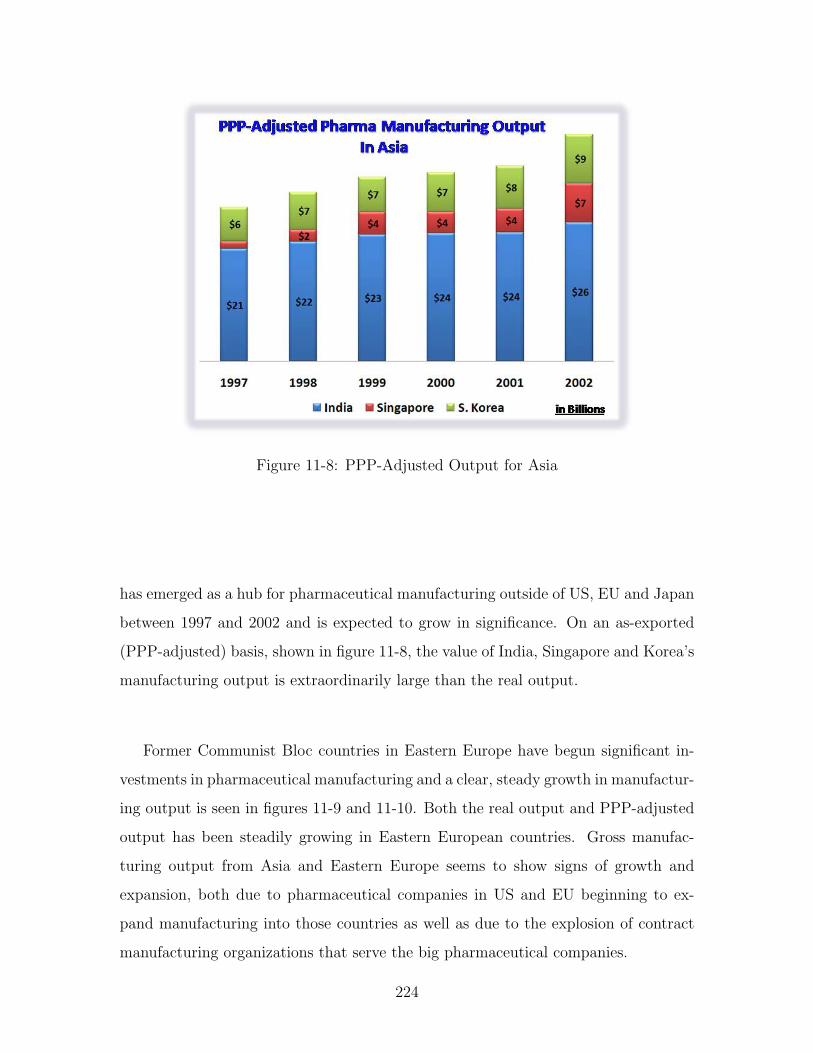
Figure 11-8: PPP-Adjusted Output for Asia
has emerged as a hub for pharmaceutical manufacturing outside of US, EU and Japan
between 1997 and 2002 and is expected to grow in significance. On an as-exported
(PPP-adjusted) basis, shown in figure 11-8, the value of India, Singapore and Korea’s
manufacturing output is extraordinarily large than the real output.
Former Communist Bloc countries in Eastern Europe have begun significant in-
vestments in pharmaceutical manufacturing and a clear, steady growth in manufactur-
ing output is seen in figures 11-9 and 11-10. Both the real output and PPP-adjusted
output has been steadily growing in Eastern European countries. Gross manufac-
turing output from Asia and Eastern Europe seems to show signs of growth and
expansion, both due to pharmaceutical companies in US and EU beginning to ex-
pand manufacturing into those countries as well as due to the explosion of contract
manufacturing organizations that serve the big pharmaceutical companies.
224

Figure 11-9: Pharmaceutical Output for Eastern Europe
Figure 11-10: PPP-Adjusted Output for Eastern Europe
225

11.2 Prior Literature
Literature on manufacturing location decisions and strategic frameworks for organiz-
ing global organizations were carefully reviewed to identify any applicable frameworks
for pharmaceutical manufacturing
11.2.1 Determinants of Manufacturing Location
Manufacturing location theories were directed towards understanding location deci-
sions made by firms seeking to minimize the cost of factor inputs (which included
the delivery cost of the manufactured goods) from the chosen location. Subsequent
theories of foreign investments and manufacturing expansions focused on identifying
the contributing factors for firm’s choice of out-of-country (particularly out-of-US)
manufacturing locations.
By dividing product life-cycle into new, maturing and standardized products, Ver-
non [99, 100] identified that the product lifecycle plays a significant role in location
decisions. The unstandardized nature of a new product like its factor inputs, man-
ufacturing process, product specifications are highly variable. The need to maintain
adequate freedom to change these characteristics defining the product (inputs, process
and specifications), relatively higher price elasticity of demand for the product given
its novelty in the market and the need to swiftly communicate and be informed by the
market precludes firms from moving manufacturing locations far off from the location
where the product was first developed. As a product matures, Vernon speculates that
the need for flexibility declines due to commitments from firms towards establishing
standards in product specifications and the manufacturing processes. Firms become
increasingly interested to invest in fixed set of manufacturing assets whence factor
costs begin to play larger role in manufacturing decisions. During this changing and
decreasingly uncertain period, manufacturing location decisions tend to move away
from the primary location where the product was developed depending on the speed
of the transition in this phase of the product cycle. Finally, as a product becomes
standardized, Vernon’s model postulates that less-developed countries might be offer-
226

ing cost competitive advantages for becoming preferred locations of manufacturing.
The standardized product and the manufacturing process give the firm the ability to
replicate the production in any location, within a certain measure of variability. The
familiarity with the market and the price competition also dictates the need for firms
to push their factor costs to more cost-efficient locations.
Subsequent studies focused on identifying the determinants of which firms pursue
foreign investments within an industry and the determinants of foreign investments
in manufacturing across industries. Horst’s [44] empirical study of the determinants
showed the impact of factors like economies of scale by virtue of firm size (viz., defined
by the firms assets), the target foreign market where the foreign investment is headed
and the profitability and experience of the firm in the production and manufacturing
of the product to be the determinants of which firms pursue foreign investments.
In a four industry study comprising of hand tools, apparel, personal computers and
electronic components, Dubois et al. [27], tested the influence of maturing product life-
cycle and process technology, market and geographic proximity, logistical complexity
and responsiveness on the decision to re-locate the manufacturing assets of a firm
in a given industry. In addition, experience and competitive priority of firms also
influenced the decision to move manufacturing assets while environment variables
like government policies, taxes, tariffs and regulations at the target locations played
a parametric role in determining location strategies in these industries.
Experience heavily affects the location decisions of manufacturing firms. In a study
analyzing 130 firms making 70,000 investments globally, Davidson [23] concluded
that while firms with limited experience in making global investments tend to limit
their subsequent investments in familiar locations they are actively operating in. On
the other hand, firms with extensive experience tend to explore and invest in more
uncertain locations and respond more efficiently to global economic opportunities.
11.2.2 Frameworks for Global Strategy
Frameworks for organizing companies globally were proposed through several works
by Porter [84], Doz et al., [26], Bartlett [3], Bartlett and Ghoshal [4], Ghoshal [35]
227

and Prahalad and Doz [87]. A sequential view of the industry, the region and the
firm were considered and the factors influencing global expansion and organization
were proposed. International managers could organize, depending on the nature of
their industry and the region specific factors, either to manage global integration or
local responsiveness. Functions that needed a local market input were high on local
responsiveness, while functions like research and development that were fairly scale
independent and needed global coordination were organized to meet global integration
as a primary goal.
Lessard [59], in extending industry level framework by Doz et al., [26], geographic
region competitiveness framework by Porter [84] and firm level organization frame-
work by Bartlett [3] and Bartlett and Ghoshal [4], proposed local to global variation
in organizing an international firm across its market spread and configuration of core
activities with the depth of the localization of its activities and the strength of the
connections of its operations. While, the aforementioned global organizing framework
considered all functions of firm, factors specific to globalization of manufacturing
were not investigated. The frameworks discussed in this work are an extension and
Lessard’s firm level internationalization, but with focus entirely on manufacturing in
pharmaceuticals and biologics.
Ferdows [30], in his factory organization model of proposed that every factory in
an organization has a purpose that the organization assigns and that every factory
has to traverse a path to become the lead factory of that company to add value to
the company’s bottom-line. In his framework, Ferdows identifies factories to be one
of six types - outpost, offshore, server, source, contributor and lead factory and these
have been shown in increasing value to the firm from bottom to top in figure 11-11.
A factory established as a minimum basic investment in a particular region to
gather market information and for keeping the organization plugged into the network
of a particular geography was termed an outpost. An outpost, according to Ferdows,
is almost always either a server or an offshore facility. An offshore location is estab-
lished with the goal of catering to the local market and present cost advantages of
selling into the local market. A server on the other hand has comparatively more
228

Figure 11-11: Ferdows [30] Model for Organizing Manufacturing Plants
freedom to improve processes and products and significantly more freedom to estab-
lish, validate and develop suppliers. A source factory, in addition to having unlimited
flexibility in defining process and product improvements, usually has limited flexibil-
ity in the development process. A contributor factory contributes significantly to the
company bottom-line by providing services similar to that of lead factory in terms
of product and process development, but is also in-line to becoming a lead factory
for the company with subsequent investments. A comparison of the various factory
types is shown in table 11.2.
In another model of coordinated manufacturing plants within a firm, Shi and Gre-
gory [92], proposed that different firms could be identified into four different types;
home exporters (for example, Boeing) where the manufacturing is in a single re-
gion or location, regional exporters (for example, pharmaceutical companies) where
manufacturing is carried out in more than one region with each region supplying
locally, globally integrated manufacturers (for example, Coca-Cola concentrate pro-
ducers and bottling companies) where manufacturing is distributed globally and the
global demand is met with an integrated manufacturing network and globally coor-
dinated manufacturers (for example, Mc Donald’s) where manufacturing is heavily
229

Figure 11-12: Shi and Gregory [92] Model for Organizing Manufacturing Plants
coordinated between different plant locations and the demand is met by varying pro-
duction between the integrated facilities as shown in figure 11-12. One of the chief
critiques of such a model is its inability to prescriptively determine which organizing
framework would best suited for a business keeping both the risks and benefits of
such an organizing framework while creating such an organization strategy.
230
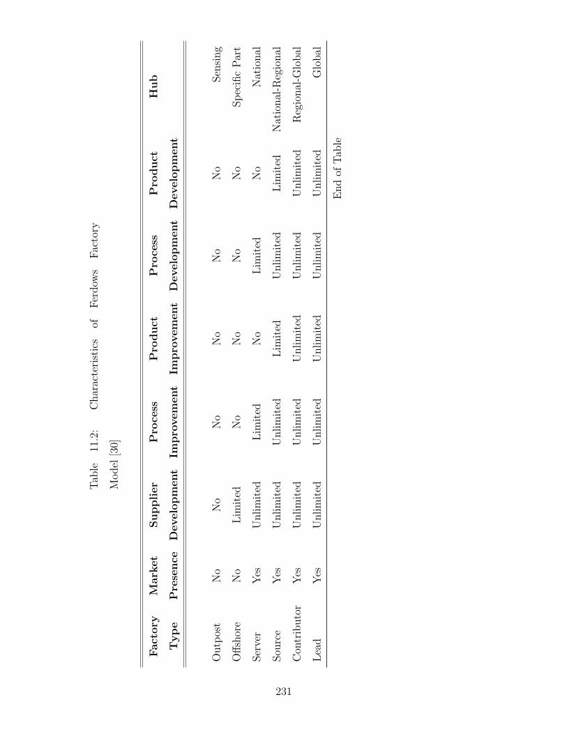
Tab
le11
.2:
Char
acte
rist
ics
ofF
erdow
sF
acto
ry
Model
[30]
Fact
ory
Mark
et
Suppli
er
Pro
cess
Pro
duct
Pro
cess
Pro
du
ctH
ub
Typ
eP
rese
nce
Develo
pm
ent
Impro
vem
ent
Impro
vem
ent
Develo
pm
ent
Develo
pm
ent
Outp
ost
No
No
No
No
No
No
Sen
sing
Off
shor
eN
oL
imit
edN
oN
oN
oN
oSp
ecifi
cP
art
Ser
ver
Yes
Unlim
ited
Lim
ited
No
Lim
ited
No
Nat
ional
Sou
rce
Yes
Unlim
ited
Unlim
ited
Lim
ited
Unlim
ited
Lim
ited
Nat
ional
-Reg
ional
Con
trib
uto
rY
esU
nlim
ited
Unlim
ited
Unlim
ited
Unlim
ited
Unlim
ited
Reg
ional
-Glo
bal
Lea
dY
esU
nlim
ited
Unlim
ited
Unlim
ited
Unlim
ited
Unlim
ited
Glo
bal
End
ofT
able
231
11.3 Objectives and Scope
There are two main objectives of this framework. First, the work proposes a global
pharmaceutical manufacturing model that has been observed so far in the market.
And second, the work proposes a new strategic lens, based on Bartlett and Ghoshal’s
framework, that a pharmaceutical or biologics company could employ to craft an
global manufacturing strategy. While the first objective identifies the path that
pharmaceutical and biologics companies have taken to reach to the current situa-
tion in global manufacturing, the latter objective builds a strategic framework that is
useful in addressing the challenges faced by companies planning on globalizing their
manufacturing plants.
The scope of this work pertains to the pharmaceuticals and biologics manufactur-
ers with a strategy to sell products in the OECD countries (especially North America,
Japan and the European Union). The manufacturing output data from UNIDO in-
dustrial statistics database [79] was limited to the available range from 1997 to 2002.
However, whenever possible, current thinking on the topic was identified by informal
interviews with professionals, managers and consultants to the pharmaceuticals and
biologics industries. Finally, this work is intended to give a prescriptive framework
for the different issues that a firm needs to think about and is in no way intended to
be predictive of what the industry is set to look like 5 or 10 years from now.
11.4 The Growing Influence of Emerging Economies
Manufacturing output growth in the emerging economies of Asia and Eastern Europe
was clearly seen in figures 11-7, 11-8, 11-9 and 11-10. However, to draw a holistic
picture we need to examine and overlay the in-country pharmaceutical demand and
demand growth with pharmaceutical manufacturing real output (unadjusted for PPP)
and output growth.
Figure 11-13 overlays the market output and market demand for the year 2002
in India, Singapore, Poland and Hungary. The market demand data were obtained
from Datamonitor industry profile reports published by Datamonitor USA [97]. We
232

Figure 11-13: Output and In-Country Market Demand for 2002
observe that in both India and Singapore, the in-country pharmaceutical market de-
mand is significantly lower than the manufacturing output. India and Singapore are
seen to be net exporters of pharmaceutical products and this can be seen as evi-
dence of expansion of manufacturing and not necessarily expansion of US/EU based
pharmaceutical companies into these countries. Manufacturing output in Poland and
Hungary were found to be lower than the in-country market demand as showing in
figure 11-13. Since these are aggregate demand and manufacturing output data, it
is important to note that these countries might be net-exporters in specific manufac-
tured pharmaceutical products or intermediates.
Figure 11-14 overlays the pharmaceutical market demand and manufacturing out-
put growth for the year 2002. Singapore has shown extraordinary growth in man-
ufacturing output in 2002 due to the specific actions of the Singapore government
towards encouraging growth of pharmaceutical manufacturing in Singapore through
various incentives that shall be discussed later on in this chapter. India exhibited
higher market demand which is believed to be related to population in India as well
as the economic growth leading to increased healthcare expenditure. Hungary and
233

Figure 11-14: Output and In-Country Market Demand Growth for 2002
Poland exhibited very close growth rates in both output and market demand meaning
that these countries might very well maintain their positions as net pharmaceutical
importers.
UNIDO INDSTAT data on pharmaceutical manufacturing establishments show
that (c.f. figure 11-15) while the number of establishments (defined as a single owner-
ship entity performing an activity in a single location) in Japan and Eastern Europe
have remained same between 1998 and 2002, the number in EU and US have been
falling considerably since 2002. At the same time, the establishments in Asia are on
the rise. It was found that this increase in Asia and other countries were not equal to
the decrease in the number of establishments in US and EU, indicating that the cost
cutting measures might be a strong impetus behind such closures since new matching
facilities were not being opened in other countries.
The number of employees in pharmaceutical manufacturing establishments pro-
vided a telling tale of how employment has been affected by the growth of manufac-
turing in Asia and other locations. Clearly, figure 11-16 shows a considerable decline
in the number of people employed in pharmaceutical manufacturing in the US, but
234

Figure 11-15: Pharmaceutical Manufacturing Establishments
the rise in employment, surprisingly is highest in Europe and not Asia or Eastern
Europe during the period 1997 to 2002. European Union employment considerably
increased during this period and is possibly due to the unionized nature of the work
force in Europe and due to the growth of Italy, Spain and Portugal as locations within
the EU where manufacturing began to pick up speed towards the end of the 1990s.
The evidence overwhelmingly points to the fact that manufacturing output is
growing without question in the emerging markets of Asia and Eastern Europe. While
it is unrealistic to expect this growth to have come solely from manufacturers in US,
EU and Japan shifting their manufacturing bases, it is very apt to expect considerable
growth in the number and exports of contract and generics manufacturers in emerging
economies.
11.4.1 Factor Cost Advantages
Countries in Asia and Europe enjoy clear factor cost advantages. In figure 11-17,
the real factor costs are shown as a fraction of the PPP-adjusted pharmaceutical
output. This analysis assumes that a company located in US or EU would be able
235

Figure 11-16: Employees in Pharmaceutical Manufacturing
to gain factor cost advantages by manufacturing at the real costs of a country in
Eastern Europe but by selling the product in the developed world. By adjusting the
pharmaceutical output with the Country PPP conversion factor, the actual value of
the pharmaceutical product could be found in order to fairly compare the factor costs
in the developed world.
The figure 11-17 shows that countries in Eastern Europe enjoy cost advantages
that are very much in line with what was found in the Asian countries like India.
A value of 10% in factor costs could be saved by manufacturing products in the
developing world and subsequently selling the products in the developed world. While
this by itself may not be a winning argument for off-shoring manufacturing or the
emergence of low-cost contract manufacturers in these developing countries, it is
nevertheless a compelling factor that contributes to the bottom-line if companies
are careful in the execution of utilizing the low cost advantage.
Another notable observation to be made from figure 11-17 is that the cost of man-
ufacturing is falling in countries like US, possibly as a combination of learning curve
effects as well as increased value capture due to growing prices of pharmaceuticals.
236

Figure 11-17: Factor Cost Percentages on a PPP basis for Eastern Europe
Figure 11-18: Factor Cost Percentages on a PPP basis for Asia
237

Figure 11-19: PPP-Adjusted Value Added Per Employee as a Percentage of that inthe US
However, if factor costs in EU countries, shown in figure 11-18, are compared with
those of US, the distinct labor cost advantage that US establishments enjoy is obvi-
ous. EU having a very high fraction of unionized work force has considerably higher
factor costs than that in the US.
11.4.2 Labor Productivity
Doubts would have to be expressed in the face of data on labor productivity about
the real value in moving manufacturing to low cost countries outside of EU and US.
While the advantages of cheaper man power cannot be easily overlooked, the fact
that the labor productivity (adjusted value added per employee as a fraction of that
contributed by an employee in the US) is abysmally low is very disconcerting if we
were to accept the assumption that eventually the cost advantages in different parts
would iron out over time.
While it is worthy to note that the extraordinary healthcare and drug costs in the
US may skew the actual value added in countries like US and EU, it is very telling to
238

observe that some of the countries only a 30% to 40% labor productivity as the US.
This brings to fore the question of low-cost advantage as a sustainable competitive
advantage for pharmaceutical companies deciding to move manufacturing to low cost
locations. As a result, it can be expected that there must be reasons other than
simply cost advantages behind why firms decide to move manufacturing to locations
outside the US and EU.
11.5 A Life-cycle Model for Globalization of Man-
ufacturing
The dependence of manufacturing location decisions taken by firms on product lifecy-
cle proposed by Vernon [99, 100] points out that lifecycle stages of the product alters
the ability of firms to take on risks of investing in new locations. A holistic perspec-
tive of manufacturing location decisions needs to take into account the industry level
constraints, firm level objectives, country level factors and product level issues.
A pharmaceutical or biologics manufacturer (referred to as the firm) disaggregates
its goal of maximizing shareholder value into market seeking and/or resource seeking
and/or efficiency seeking objectives whereby the firm maximizes expected returns for
a given level of underlying, undiversifiable risk. The magnitude of the importance
that the firm places on the three independent objectives, the ability and the appetite
of the firm to undertake risk, and the lifestage of the firm, its products and its markets
significantly set the direction and strategy of the firm.
Conceivably, at an early stage of product development, the firm, following Ver-
non’s [99, 100] model, look for talent (resource) and customers (market). At this
stage, the undiversifiable risk of product failure looms large on the firm and the firm
is heavily invested in bringing the first product to market. As the product begins to
diffuse into the market reaching peak sales, the firm begins to shift emphasis, much
like in Vernon’s model, to better resources while learning to manage said resources
efficiently. Finally, a mature, generic product would have its premium price position
considerably eroded and the onset of price competition forces firms to seek for higher
239

efficiencies. In addition to the aforementioned objectives and risk appetite of the firm,
exogenous factors like government regulations and policy both places constraints and
presents opportunities for firms. For example, while stringency of safety regulations
presents unavoidable constraints on the firm, government tax policy, incentives for
relocation and investment and so on present opportunities for value creation by the
firm. The rest of the section will focus on the implications of this lifecycle based
location model for pharmaceuticals and biologics.
11.5.1 Model for Pharmaceuticals
After a target has been identified as a cause of a particular medical condition or
disease pharmaceutical companies screen their in-house chemical compound libraries
to attack the target in order to cure the condition. These optimized leads, called New
Chemical Entities or NCEs, that attack the target is then optimized by synthetic
chemistry and are tested for efficacy in animals. When the safety profile of the NCE is
satisfactory based on animal trials, the companies begin human clinical trials in three
phases. At the end of each phase, the product is approved by the FDA depending on
the data from that stage and the company can begin selling the product after passing
scrutiny in all stages. The main challenge here is that the timeline when the patents
on the NCE expire and the timeline for drug product approval leave very little wiggle
room for pharmaceutical companies to extract value from successful, blockbuster
drug products. As soon as patents expire, a number of generics manufacturers enter
the market and the gross margins and market share of the original innovator of the
product are driven down.
As the lifecycle of the NCE progresses from being patented to subsequent loss of
patent protection, the manufacturing technologies and locations change. To begin
with, when the NCE enters the market as a drug product, its manufacturing predom-
inantly occurs in US, EU or Japan. Although, in the recent past, some intermediates
are being outsourced from contract manufacturers, this has been a relatively new
development. As the product nears patent expiration, generic companies begin to
prepare for entry and most usually have locations outside of the first location. As
240

Figure 11-20: Global Expansion Model for Pharmaceutical Manufacturing
Figure 11-21: Global Expansion Model for Biologics Manufacturing
241

the patent expires, prices and market share take a hit and the gross margins on the
product begin to fall, as shown in figure 11-20. This movement in gross margins
might also force the original innovator of the NCE to move manufacturing to newer
locations to save on the cost of goods sold on this pharmaceutical product. During
this period of transition of manufacturing from high cost to a low cost location, as
shown in figure 11-20, another NCE with higher gross margins might be introduced
in the original location (for example in the US) causing another cycle to begin for
that product.
11.5.2 Model for Biologics
A different model for biologics needs to be proposed. The biggest challenge in propos-
ing such a model for biologics manufacturing is with the fact that while pharmaceu-
ticals have seen more than 50 years of innovation based business models, biologics
have been around for less than 30 years now. In addition, pharmaceutical generic
product approvals have been ironed out a long time ago, compared to the follow-on
biologics approval regime in the US (which is still in the making as of May 2008).
Therefore, since cost-based manufacturing pressures have not yet hit biologics, manu-
facturing had been limited to US, EU and Japan thus far. However, tax holidays and
growing expertise in India, Ireland and Singapore have been encouraging biologics
manufacturers to look outside the US and EU for their manufacturing needs. Never-
theless, current thought indicated that given the extraordinary fixed costs of biologics
manufacturing, the manufacturing capacity in US and EU would always be put to
use in order to decrease the average cost of manufacturing biologics. As a result,
the proposed model, in figure 11-21, shows that as gross margins tend to decrease,
manufacturing of biologics would still be carried on in the location where the product
innovation was first carried out (US in a large number of cases). It is as yet unclear
what the future state of biologics manufacturing would be, if the US were to begin
approving follow-on biologics.
242

11.6 A Framework for Global Manufacturing Strat-
egy
Following Lessard’s [59] extension of the strategic global organizing framework pro-
posed by Porter [84], Doz et al., [26], Bartlett [3], Bartlett and Ghoshal [4], Ghoshal [35]
and Prahalad and Doz [87] organizing framework for global strategy, the firm’s indus-
try is analyzed for identifying its globalization potential with a focus on manufactur-
ing. Following this, geographic region level framework for making strategic location
decisions is presented.
11.6.1 Industry Level Framework
Four key factors need to be considered before deciding whether a particular industry
is set to extract value from globalization than another. This industry-framework
captures economies of scale and scope and the level of risk (related to both technology
transfer and intellectual property infringement) and stringency of regulations on that
industry. Four industries - beverages, pharmaceuticals, biologics and airplanes - have
been compared on a spider web diagram in figure 11-22.
11.6.1.1 Scale
Economies of scale refer to the decrease in average cost as the scale of production
increases. While this is almost always true, demand constraints limit the economies
of scale that can be achieved by global expansion of manufacturing. For example,
the beverage industry can highly utilize the economies of scale by expanding its
manufacturing (bottling) to far away regions across the globe in order to be very
close to markets and receive instant demand profiles of the local market. However,
for an industry like airplanes it would be unwise to build manufacturing sites at more
than one location, given that the overall demand in the world is constrained and that
a new facility entails huge capital investment making it difficult to recover the fixed
costs effectively.
Construed another way, a beverage manufacturer can decrease the average deliv-
ered cost of a finished product when manufacturing is spread out across the markets
243

Figure 11-22: An Industry-Level Framework for Global Manufacturing Strategy, Ex-tension from [59]
being served. Clearly, for this to be true the fixed costs of manufacturing at multiple
locations across the globe should be less than the lost market demand due to the
firm’s inability to supply efficiently. In the case of pharmaceuticals and biologics,
the initial capital expenditure is significantly higher than that in beverages. This
makes it unattractive for firms to pursue building multiple locations for the same
pharmaceutical or biologics product. However, as seen in the figure 11-22, biolog-
ics manufacturing facilities are significantly more capital investment intensive than
pharmaceutical facilities and hence have much less attractive economies of scale [13].
11.6.1.2 Scope
Economies of scope refer to the decrease in average cost as the scope (number or vari-
ety) of products manufactured at a given manufacturing facility or location increases.
Clearly, global expansion plays well with industries where the number of products
tends to be higher than usual. The beverage industry sells 7 to 8 flavors of bever-
ages that can be manufactured at a single location. Therefore, this product scope
244

in manufacturing spreads the fixed cost of manufacturing across different products
and is allows for beverage manufacturers to explore new locations that serve multiple
products to the local market.
Pharmaceutical and biologics manufacturing facilities, on the other hand, have sin-
gle product manufacturing faciliites. Between these two sub-industries, the relatively
easier to replicate chemical synthesis based pharmaceutical manufacturing facilities
are usually more broader in product scope than the dedicated manufacturing facilities
used by biologics manufacturers as seen by the increased favorability in the industry
level framework in figure 11-22. Clearly, the minimal scope of airplanes severely limit
the manufacturing location product scope in the case of the airplane manufacturers.
11.6.1.3 Risk
Presence of substantial risk in the business environment, in the process of bringing
products successfully to market, in ensuring product success in the market, in tech-
nology transfer, and in intellectual property infringement pose significant hindrances
discouraging globalization of manufacturing. The beverage industry, perhaps, has the
most amenable risk profile given the least uncertainty in technology transfer of man-
ufacturing, least risk in market share losses because of strong brand differentiation
and conspicuous lack of intellectual property risks (notwithstanding trade secrets).
In the case of airplane manufacturers, while technology transfer risks are very large,
the intellectual property assoicated with the airplanes is well protected by means of
the capital intensive nature of the business.
Pharmaceuticals and biologics manufacturers exhibit riskier profiles towards glob-
alization of manufacturing. In the case of pharmaceuticals, while the capital in-
vestments are significant, competitors can raise sufficient capital easily to invest in
pharmaceutical manufacturing facilities. However, intellectual property infringement
risks are very prevalent in this sector, especially in emerging economies that are en-
tering the WTO patent protection regime. Given the nature of the manufacturing
process, as discussed before, pharmaceutical manufacturing poses very low risk of
technology transfer.
245
The risk profile of biologics manufacturers is starkly different from pharmaceu-
ticals. There are substantial technology transfer risks in moving manufacturing lo-
cations. Many manufacturing processes that are apparently well characterized are
hardly replicatable even by the firm that had developed it in the first place. Compli-
cations in technology transfer and process qualification, validation and process control
probably are the single biggest risk that biologics manufacturers have to mitigate in
their decision to globalize manufacturing. While intellectual property infringement
risks are lower compared to pharmaceuticals, growing educated demographic in Asian
countries and a new-found love in the life sciences in these countries might change
how firms perceive intellectual property risks in the process of globalization of man-
ufacturing.
11.6.1.4 Regulations
Industries that are mandated to adhere to stringent regulations, standards and prac-
tices usually are not incentivized to expand their manufacturing globally, unless such
standards and regulations are globally harmonized and reconciled or the firm has
more and better experience in managing multiple country and regional regulations
and standards. In general, firms are better of adhering to the common minimum
standards across the entire manufacturing assets in order to be able to hold the op-
tion of moving manufactured goods from any location to any location. Even within
this perspective, a firm with headquarters in the US versus a firm operating with the
US as primary location might
A heavily regulated industry like pharmaceuticals or biologics is much less amenable
to globalization than beverage manufacturing. The general rule that many pharma-
ceutical companies in the US follow is to meet more than the common minimum
regulatory standards across the different markets and locaitons these firms operate
in so that the chance of failing to meet regulations is minimized. Such policies would
not only increase the fixed costs in building such safeguards, but also increases the
monitoring costs on the firm deciding to globalize manufacturing. Notably, pharma-
ceuticals and biologics manufacturers have been very expansive in spite of differing
246

Figure 11-23: A Geographic Region Level Framework for Global Manufacturing Strat-egy
regulations between countries, in part because of their comfort in meeting US, EU and
Japanese standards and regulations and also because of the increasing harmonization
of the standards and regulations at other locations.
11.6.2 Geographic Region Level Framework
On geographic level, firms need to think of five different sets of criteria in order to
devise a strategy for global manufacturing shown in figure 11-23. These factors can be
grouped as - Factor cost advantages, regional/country policies, taxes and regulations,
regional/country risk, infrastructure and availability of skilled human resources and
expertise in the region or country.
11.6.2.1 Factor Cost Advantages
On-going operating cost advantages will play a significant role in determining whether
a firm would build manufacturing at a particular location or not. From the UNIDO
INDSTAT data [79], factor costs of Asia/Eastern Europe were found to be at least
10% lower than those in the US (c.f. figure 11-17) and up to 50% lower than those
in EU countries (c.f. figure 11-18). While these factor cost differences are attractive
for firms looking to explore new regions, it must be cautiously mentioned that factor
247

cost advantages do not mean that moving manufacturing will be value additive to the
firm’s bottom-line. At the same time, firms would never move manufacturing to high
cost countries or countries with high growth rates in factor costs.
For biologics, it is worth mentioning the consumables for downstream processing
plays a larger role in determining factor costs and since consumables almost exclu-
sively are imported from US and EU, the advantages in materials cost is substantially
lesser. In addition, employees in biologics manufacturing are considerable more edu-
cated, decreasing the cost differential further, than in pharmaceutical manufacturing.
Finally, storage and transportation costs are substantially lesser for pharmaceuticals;
the requirements on cold chain capabilities would mean that biologics manufacturers
might have to consider building those capabilities in countries where such capabilities
are underdeveloped.
11.6.2.2 Tax Policy and Regulations
Tax holidays and reduced tax rates allow big pharmaceutical and biologics companies
to add substantial value to their bottom-line. Tax holidays are provided by national
governments to help jumpstart the local economy in a particular industry or sector
depending on the local needs and aspirations. The successful examples of tax holiday
countries include Puerto Rico (where the tax holiday status expired in 2006 for phar-
maceutical companies), Ireland (where the tax rate is currently at 10% and is set to
increase to 12.5% in 2010) and Singapore where the tax rate for manufacturers has
been 0%.
The following example shows how tax advantages arise in moving to low tax
location. Consider a blockbuster drug with $1 billion in non-US revenues. With 25%
cost of goods sold (COGS), the pre-tax income for the product would be $750 million
shown in table 11.3. If this were to be taxed at US tax rates (35% corporate tax
rate), this tax would be amount to $262.5 million. If the tax rate were to be 10%
as in Puerto Rico, the tax on this would amount to only $75 million, a tax savings
of $187.5 million on a yearly basis. Assuming 0% growth in revenues and COGS,
and a 15% weighted average cost of capital for a company like Pfizer or Merck, this
248
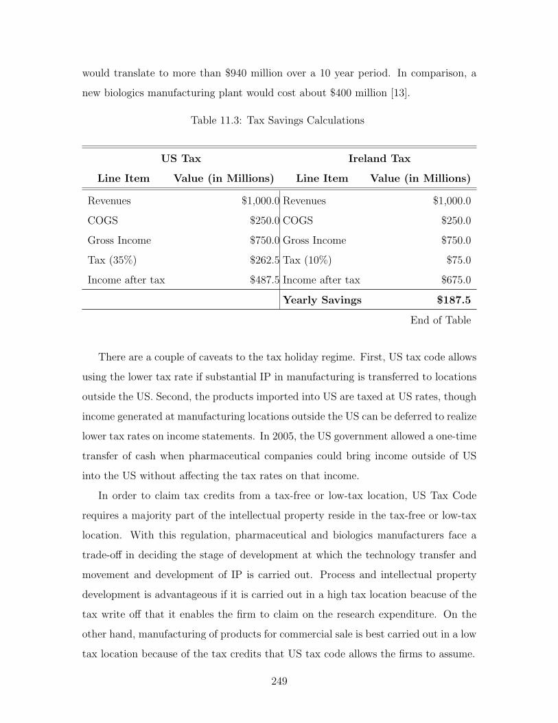
would translate to more than $940 million over a 10 year period. In comparison, a
new biologics manufacturing plant would cost about $400 million [13].
Table 11.3: Tax Savings Calculations
US Tax Ireland Tax
Line Item Value (in Millions) Line Item Value (in Millions)
Revenues $1,000.0 Revenues $1,000.0
COGS $250.0 COGS $250.0
Gross Income $750.0 Gross Income $750.0
Tax (35%) $262.5 Tax (10%) $75.0
Income after tax $487.5 Income after tax $675.0
Yearly Savings $187.5
End of Table
There are a couple of caveats to the tax holiday regime. First, US tax code allows
using the lower tax rate if substantial IP in manufacturing is transferred to locations
outside the US. Second, the products imported into US are taxed at US rates, though
income generated at manufacturing locations outside the US can be deferred to realize
lower tax rates on income statements. In 2005, the US government allowed a one-time
transfer of cash when pharmaceutical companies could bring income outside of US
into the US without affecting the tax rates on that income.
In order to claim tax credits from a tax-free or low-tax location, US Tax Code
requires a majority part of the intellectual property reside in the tax-free or low-tax
location. With this regulation, pharmaceutical and biologics manufacturers face a
trade-off in deciding the stage of development at which the technology transfer and
movement and development of IP is carried out. Process and intellectual property
development is advantageous if it is carried out in a high tax location beacuse of the
tax write off that it enables the firm to claim on the research expenditure. On the
other hand, manufacturing of products for commercial sale is best carried out in a low
tax location because of the tax credits that US tax code allows the firms to assume.
249

In the case of pharmaceuticals, given the nature of intellectual property and the
technological complexity of the process, a pharmaceutical manufacturer would incur
very minimal technology transfer cost when this technology transfer is carried out at
later stages of product development (during Phase III clinical trials, for example).
This implies that the trade-off that manufacturing strategy managers face is more
inclined towards investing in process development in a high tax location, claiming tax
credits on the research and development expenditure, then incurring some technology
transfer costs in moving the manufacturing process to a low tax location.
In the case biologics, given the nature of technological complexity of the process
and difficulties in replicability, late stage process technology transfers are signigicantly
risky, time consuming and expensive. On the other hand, by choosing to develop the
manufacturing process and carrying the process development in a low-tax location,
the firms leave valuable research and development tax credits on the table. In addi-
tion, given that biologics process development is more complex and needs a stronger
connectedness (as defined by Lessard [59]) with the product and clinical research
groups, transfering process development to a low-tax location early on in the product
life cycle might prove to be a very risky proposition.
In-country manufacturing and environmental regulations play a critical role in
determining the attractiveness of a particular location. First, the stringency of such
regulations and sophistication of the regulatory bodies determines the difficulty level
in receiving timely approval from national regulatory bodies. In recent times, many
attractive manufacturing destination countries have begun to emulate or harmonize
their regulatory regimes in alignment with the US FDA or the European EMEA.
Secondly and more importantly, the closer the regulatory standards to the US stan-
dards, the better the local expertise in understanding and following US regulations
in the manufacturing sites of those countries. Governmental incentives in the form
of land grants, sponsored training programs, matching capital investments, utility
supply guarantees etc. are some other incentives that attract pharmaceutical and
biologics manufacturers to relocate their facilities to these countries.
250

11.6.2.3 Country risk profile
Idiosyncratic country risks that cannot be diversified away play a significant role in
determining which locations pharmaceutical firms choose not to explore for manu-
facturing. Examples of non-diversifiable idiosyncratic risks include Puerto Rico for
hurricanes, Singapore for earthquakes and tropical storms, China for political risk, In-
dia for IP risk and so on. There are some other idiosyncratic risks (like exchange rate
risk and inflation risk) that can be diversified away by proper hedging mechanisms.
In addition to the country specific risks, pharmaceutical companies also need to
look at addressing supply risk by choosing one location as a sole supplier of a particular
API. Most pharmaceutical companies source intermediates and APIs from more than
one location in order to hedge the bets on supply risk.
11.6.2.4 Infrastructure
The presence of developed infrastructure to ensure continuous supply is an important
criterion firms could use to identify the locations for manufacturing. Infrastructure
includes the hard, physical infrastructure like roads, uninterrupted utilities and ser-
vices, living conditions and finally the legal infrastructure. Access to uninterrupted
utilities and services are very critical for pharmaceutical and biologics manufactur-
ing. For example, the fact that Singapore receives its water supply from Malaysia
is a critical criterion that firms need to think about when deciding locating plants
in Singapore. Access to transport infrastructure is important, not only to transport
materials but also allow people to commute or reach their workplaces uninterrupted.
A large number of biologics manufacturing companies would need to send em-
ployees from US and EU as expatriates to the manufacturing locations for training,
installation, validation and commissioning and operation of the plant. In such cases,
the living conditions and the ability of the local population to communicate in En-
glish plays an important role for unhindered operation of the plant. Finally, legal
infrastructure including an efficient police and security force and a stable legal sys-
tem would be considered in determining the location of a manufacturing plant. The
ability to gather land grants from landowners will also play a role in determining the
251

viability of a particular location.
11.6.2.5 Knowledge and Skills of Local Population
Pharmaceutical and biologics companies have differing requirements in terms of em-
ployee education levels. An average pharmaceutical manufacturing employee might
simply have to be able to read standard operating procedures and write batch records
while an employee in biologics manufacturing might need to know the science and
reasoning behind the process. For this reason, an average employee in biologics man-
ufacturing is expected to be a college graduate (80% college graduates in biologics
manufacturing). Therefore, access to and availability of educated human resources
would have to be considered especially in the case of biologics manufacturing.
The growing population of graduates and post graduates in India and China is
a testament to the growing supply of qualified labor that is increasingly demanding
challenging opportunities. The growth of contract manufacturing organizations in
India has been banking on the rise of these graduates from numerous science and
engineering colleges in India. India, Singapore and Ireland are at an advantageous
position as English is the preferred language of communication and is widely spoken
in these countries. The interest of employees in US and EU to go to manufacturing
locations as expatriates is also dependent on the infrastructure, cultural and phys-
ical proximity to the Western world, the school system and the facilities near the
manufacturing location and is a factor to be considered if there is no substantial
at-the-location expertise.
11.6.3 Deriving Implications of the Framework on BiologicsCompanies
In an attempt to test the framework’s validity, the strategic directions and implica-
tions of the manufacturing locations and positions of top 5 biologics companies by
revenue were studied. These biologics companies have had rich, distinct histories since
Genentech was founded in 1976 kickstarting the biotechnology industry. Amgen, Inc.,
Genentech, Inc., Novo Nordisk A/S, Genzyme Corporation and Biogen Idec, Inc were
252

the top product revenue companies in the biologics sector shown in table 11.4. The
revenue, %US Sales, Cost of Sales, Tax rate and the manufacturing facilities were
all gathered from the Form 10-K EDGAR filings of these companies from the US
Securities Exchange Commision website.
Amgen and Genentech had revenues that were predominantly based on US sales,
while Genzyme, Novo Nordisk and Biogen had more than 40% non-US sales. The
skewed share of US based sales at Amgen and Genentech are a direct result of some
of the marketing arrangements these pioneering companies had to enter into with big
pharma companies like Johnson & Johnson, Roch and Wyeth. Non-US Revenues from
Amgen’s top two drugs are shared with Johnson & Johnson and Wyeth Biopharma.
Genentech’s products are marketed outside of the US by Roche’s pharmaceutical
subsidiary based in Basel, Switzerland.
Cost of sales (a measure of the labor and materials cost of manufacturing) are
in the lower range for Amgen, Genentech and Biogen Idec. These values are at the
lower end of the expected 15%-25% of product revenues. Such lower end cost of sales
might arise from premium pricing of their products, efficiency in manufacturing or
better factor cost optimization. It is difficult to identify the real cost advantage that
these companies realize in their operations.
Tax rates as measured from the income statements of these companies make a
telling argument on the companies strategies to manufacture in low-tax locations.
The observations made by Grubert and Mutti [38] on the movement of firm incomes
to low tax or tax holiday locations seem to be effectively explaining the lower taxes
at Amgen and Novo Nordisk. The locations of manufacturing for Amgen’s primary
blockbuster products are based in Puerto Rico and until recently being developed in
Ireland. The tax rates of other biologics companies were significantly higher than
that of Amgen signaling that closely managed tax savings strategy is being employed
at Amgen.
It is interesting to note that if we trace the taxes on the products sold by Genentech
outside of the US and hypothetically compute the tax rate of Genentech’s product
line as if Genentech owned all teh rights to market the product, we might specu-
253

Figure 11-24: Strategic Implications Based on Proposed Framework
late consisderable reduction in Genentech’s effective tax rate. The effect of Roche’s
52% equity stake in Genentech, coupled with non-US marketing rights of Genentech’s
products by Roche, the tax rates for this hypothetical case might be lower the current
value for Genentech at 37.4%. Genentech has also secured an option to buy a plant
being built by Lonza in Singapore that is expected to be commisssioned by 2010.
This marks a diversion from Genentech’s all-US manufacturing strategy and its im-
plications are yet to be studied. However, in biologics it is very important to note
that only microbial fermentaion is usually relocated and mammalian cell synthesis is
still closely operated in US Locations.
254

Tab
le11
.4:
Top
Rev
enue
Gen
erat
ing
Bio
logi
csC
ompa-
nie
sof
2007
Am
gen
Genente
chN
ovo
Nord
isk
Genzy
me
Bio
gen
Idec
Pro
duct
Revenues
$14.
31B
$9.4
4B$6
.35
B$3
.46B
$2.1
4B
%U
SSale
s80
%10
0%31
%52
%56
%
Cost
of
Sale
s17
.8%
16.7
%24
.7%
20.7
%15
.7%
Eff
ect
ive
Tax
Rate
20.1
%37
.4%
28.6
%34
.7%
29.9
%
US,
Puer
toR
ico
Cal
ifor
nia
Den
mar
k,
US
Bel
gium
,U
SC
alif
ornia
Loca
tions
Net
her
lands
Sin
gap
ore1
Bra
zil,
Jap
anIr
elan
dN
orth
Car
olin
a
Irel
and
2C
hin
a,F
rance
Fra
nce
Net
her
lands3
End
ofT
able
1C
omm
issi
onin
gpl
anne
dby
2010
2D
isco
ntin
ued
in20
073C
omm
issi
onin
gpl
anne
dby
2009
255

The strategic implications based on the criteria proposed in the framework dis-
cussed in the previous section are shown in figure 11-24. The high margin nature of
Amgen, Genentech, Biogen’s products market proximity and access take precendence
over cost efficiency. Novo Nordisk increasingly faces pressure in its insulin-based mar-
kets with the threat of price competition from rival Eli Lilly and local manufacturers
of generic recombinant Human Insulin. At Genzyme, the orphan status of the top
selling drug shifts the emphasis from cost efficient to timely delivery of the product
to the patient. Therefore, the speculatin is that cost of sales is a driving factor in de-
termining the location for manufacturing and subsequently selling products at Novo
and to a lesser level at Genzyme and at the least level at Amgen, Genentech and
Biogen.
Tax strategies varied significantly between companies discussed here. Amgen ag-
gressive pursuit of generating shareholder value out of tax savings has substantially
paid off with its comparably low tax rates at 20%. Genentech and Biogen Idec seem to
have a different view on tax savings and have predominantly US tax rates for all their
sales. Genzyme, in spite of its presence in certain low tax locations, is yet to book
lower tax rates. It is speculated that Genentech, Genzyme and Biogen consider tax
as an integral fabric of reaching out to their consumers as a a good corporate citizen.
However, it should be duly noted that given Genentech and Biogen’s new manufac-
turing facilities in Singapore and Netherlands, the tax strategy of these companies
mught be seeing some changes.
The perspectives of these companies on how technology transfer risk, undiversi-
fiable country risk and supply chain risk should be mitigated vary from controlled
utilization of contract manufacturers with active demand and capacity planning (e.g.
Amgen),to Genentech and Biogen’s collaborative manufacturing and sharing the risk
of getting products to patients. Novo’s disaggregation of its manufacturing into sin-
gle bulk sourcing and multiple product formulation facilities essentially diversifies the
risk of a single location being hit by some uncertain event. Genzyme’s inclination to
carry out operations close to the market with demand would let us to speculate that
ensuring reliability in supply of products is an important aspect of Genzyme’s risk
256

mitigation strategy.
The infrastructure and human resource strategies were found to be similar across
these different companies. Technolgically intense biologics manufacturing process de-
mands well educated graduate and post-graduate work force unlike small molecule
pharmaceutical manufacturing. Proximity to Western culture helps in securing expa-
triates willing to travel, live and train the local talent at their manufacturing locations.
Knowledge and training in current Good Manufacturing Practices (cGMP) are criti-
cal in any company. Reliable infrastructure, utilities, land access, transportation and
cold chain capabilities
Finally, historical perspectives of the current position of these companies clarifies
the question of whether particular location decisions were strategically made and
organically grown or whether an acquisition allowed the firm access to a new location
that was not in the portfolio before. In addition, the global focus of Genzyme and
Novo from early stages of product development is a differentiating feature from Amgen
and Genentech where most initial sales and business was in US and EU.
11.7 Case Studies on Applying the Framework
Two case studies are shown below on the methodology of applying the proposed
framework. One company, Amgen, has substantial revenues generated globally, but
certain historic and product license constraints have not yet opened worldwide sales
opportunities at the moment for Amgen. On the other hand, Novo Nordisk had been
an international company with 99% of sales coming from outside of Denmark, the
home country. It is hoped that these cases will show the usefulness and relevance of
the Framework for organizing Global Manufacturing in Biologics. In pursuing this
analysis, a set of five regions/countries have been examined - US/EU, Puerto Rico,
Ireland, Singapore and India.
11.7.1 Location Decision for Amgen
Assuming US as the basis for factor costs, evidence points to at least 10% factor cost
advantage in Singapore and India. However, given Singapore’s growth in investments
257
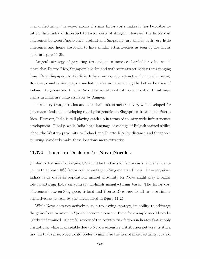
in manufacturing, the expectations of rising factor costs makes it less favorable lo-
cation than India with respect to factor costs of Amgen. However, the factor cost
differences between Puerto Rico, Ireland and Singapore, are similar with very little
differences and hence are found to have similar attractiveness as seen by the circles
filled in figure 11-25.
Amgen’s strategy of garnering tax savings to increase shareholder value would
mean that Puerto Rico, Singapore and Ireland with very attractive tax rates ranging
from 0% in Singapore to 12.5% in Ireland are equally attractive for manufacturing.
However, country risk plays a mediating role in determining the better location of
Ireland, Singapore and Puerto Rico. The added political risk and risk of IP infringe-
ments in India are undiversifiable by Amgen.
In country transportation and cold chain infrastructure is very well developed for
pharmaceuticals and developing rapidly for generics at Singaprore, Ireland and Puerto
Rico. However, India is still playing catch-up in terms of country-wide infrastrucutre
development. Finally, while India has a language advantage of Enlgish trained skilled
labor, the Western proximity to Ireland and Puerto Rico by distance and Singapore
by living standards make those locations more attractive.
11.7.2 Location Decision for Novo Nordisk
Similar to that seen for Amgen, US would be the basis for factor costs, and allevidence
points to at least 10% factor cost advantage in Singapore and India. However, given
India’s large diabetes population, market proximity for Novo might play a bigger
role in entering India on contract fill-finish manufacturing basis. The factor cost
differences between Singapore, Ireland and Puerto Rico were found to have similar
attractiveness as seen by the circles filled in figure 11-26.
While Novo does not actively pursue tax saving strategy, its ability to arbitrage
the gains from taxation in Special economic zones in India for example should not be
lightly undermined. A careful review of the country risk factors indicates that supply
disruptions, while manageable due to Novo’s extensive distribution network, is still a
risk. In that sense, Novo would prefer to minimize the risk of manufacturing location
258
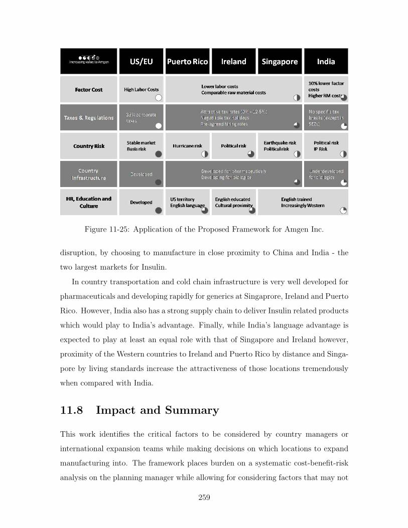
Figure 11-25: Application of the Proposed Framework for Amgen Inc.
disruption, by choosing to manufacture in close proximity to China and India - the
two largest markets for Insulin.
In country transportation and cold chain infrastructure is very well developed for
pharmaceuticals and developing rapidly for generics at Singaprore, Ireland and Puerto
Rico. However, India also has a strong supply chain to deliver Insulin related products
which would play to India’s advantage. Finally, while India’s language advantage is
expected to play at least an equal role with that of Singapore and Ireland however,
proximity of the Western countries to Ireland and Puerto Rico by distance and Singa-
pore by living standards increase the attractiveness of those locations tremendously
when compared with India.
11.8 Impact and Summary
This work identifies the critical factors to be considered by country managers or
international expansion teams while making decisions on which locations to expand
manufacturing into. The framework places burden on a systematic cost-benefit-risk
analysis on the planning manager while allowing for considering factors that may not
259

Figure 11-26: Application of the Proposed Framework for Novo Nordisk A/S
directly enter into a financial model. The framework also provides a platform for risk
assessment by planning managers that can be used as a continuous assessment tool to
identify the potential problems and pitfalls in international manufacturing expansion.
The strategy implications point out to two predominantly occuring patterns - tax and
other incentives are heavily skewed towards attracting foreign investments into regions
and that risk appetite, assessment and mitigation plays the second significant role in
determining, or at least narrowing down location choices.
In summary, it is very important to note that while factor costs are given primary
importance and attributed as the reason behind manufacturing shifting or expand-
ing into newer locations outside of US and EU, it is definitely not the only criterion
that firms must use in identifying the need to expand manufacturing globally. Tax
incentives and other factors like legal and physical infrastructure and language also
play critical roles in determining a successful location for pharmaceutical and biolog-
ics manufacturing. In biologics manufacturing, considerable history of expansion is
absent both because of the recent nature of the industry and also because of tech-
nological and financial reasons of recouping investments from existing manufacturing
260
infrastructure. Application of the geographic level strategic decision framework in-
creasingly pointed to locations where the risk benefit trade-off matched the expected
returns of the firms. Finally, patent expirations in pharmaceuticals have facilitated
the entry of newer generics companies that have sprung up in low cost countries in the
past 10 years. The scenario is expected to push more towards an even lower cost base
and drive margins further down. Pharmaceutical manufacturers will need a frame-
work like the one presented here with which they can examine and make strategic
location decisions.
11.9 Acknowledgments
I would like to express special thanks to Ms. Judy Lewent, Former CFO, Merck; Mr.
Mark Bamforth, SVP of Operations, Genzyme; Mr. Bill Rich, GM of International
Operations, Amgen; Mr. Brandon Smith, Director of Corporate Strategy, Amgen;
Ms. Leslie Prince Rudolph, International Manufacturing Strategy Manager, Eli Lilly;
Mr. Eric Cheslek, Manufacturing Strategy Manager, Eli Lilly; Dr. Mickey Koplove,
Vice President, Wyeth Biopharma; Ms. Suzanne Sensabaugh, VP MDS Biopharma;
Dr. Arun Chandavarkar, COO, Biocon India; Mr. Rakesh Bamzai, VP of Marketing,
Biocon India; and Dr. Harish Iyer, GM of Research, Biocon India for their inputs,
discussion and feedback on this chapter.
261

262
Chapter 12
Conclusion
Continuous manufacturing addresses some of the critical problems faced by secondary
pharmaceutical manufacturing, around efficiency, scale-up, quality assurance and
cycle-times. Instead of comparing the performance of continuous vs batch opera-
tions, continuous manufacturing should be viewed as an alternative design choice
available for process design in pharmaceuticals. Blending was identified as the criti-
cal last step where variance can be altered to make or break the product by affecting
prodcut quality.
Investigation on continuous blending began by a thorough literature review in this
area. The literature review revealed lack of experimental investigations on cohesive
powders in continuous blending and an understanding of the effect of microscopic
particle parameters on the performance of continuous powder blending processes. It
was also shown in literature that the system comprising of the feeding (dispensing)
system and continuous blender should be studied as one single entity as the perfor-
mance of the continuous blender is strongly dependent on the efficacy of the feeding
system.
A framework was created to understand phenomena in continuous blending and
relate it to operational variables and material properties. Flow behavior of powders
in blenders were studied by measuring residence time distributions of particles in
continuous blenders. A process model based on integrating the flow behavior and
disturbances introduced at the feeder was used in understanding the process operating
variables.
263

Continuous blending at pilot plant scale was shown to achieve blend qualities that
are mandated by FDA for safety and efficacy. Also, the effect of energy input through
rotation rates of moving elements in the blender was shown to positively affect the
blending process.
Mean residence time coupled with the disturbance frequency (or time period of
feeder fluctuation) were the two most significant operational variables that affect
blender performance. Most other independent operational variables like energy input,
flow rates angles of incline and dependent operational variables like fill weight affect
the blending process through mean residence.
Increase in particle size was shown to increase the axial dispersion coefficient of
the material in the blender. Increased dispersion coefficients were shown to increase
blender performance. A decrease in cohesive forces caused increased blender perfor-
mance. This effect was evident when the particles of different cohesion and adhesion
forces were mixed in the blender. Increased Cohesion and adhesion decreased the
axial dispersion coefficient. Change in particle shape did not exhibit a strong effect
on blender performance but did effect the fill weight in the blender considerably.
Multicomponent blending was demostrated in the pilot-scale experiments. Addi-
tion of lubricant after mixing decreased the cohesion forces and caused the blend to
segregate and blend quality to deteriorate. Lubricant coated the API and excipients
with a fine layer of small particles that reduced the cohesion forces in the particles
and increased the potential for segregation.
Identifying of an correct scale of scrutiny in powder blending leads to the cor-
rect assessments on continuous powder blending. Taking moving averages of process
monitoring data was shown to be equivalent to offline sample collection and analysis.
Theoretical predictions of blender performance were shown to be in agreement with
experiments after taking into account the variation in the powder flow behavior in
the blender.
This work advanced the knowledge on the behavior of particles in continuous mix-
ing systems. The effects of particle parameters in continuous blenders were hitherto
unknown and this thesis contributed to the scientific understanding of particle and
264

operational parameters on blending performance. This thesis also created a design
framework for the pharmaceutical industry to investigate and implement continuous
blending in particular and continuous processing in general in secondary pharmaceu-
tical manufacturing.
265

266
Appendix A
Nomenclature
API Active Pharmaceutical Ingredient
VRR Variance Reduction Ratio
RSD Relative Standard Deviation
MRT Mean Residence Time
RTD Residence Time Distribution
FDA Food and Drug Administration
PLS Partial Least Squares Regression
MLR Multiple Least squares Linear Regression
NIR Near infra-ref spectroscopy
LIF Light Induced Fluorescence
DCL Direct Compressible Lactose
MCC Micro Crystalline Cellulose
RPM Rotations per minute
NCE New Chemical Entity
MgSt Magnesium Stearate
A Normalization Constant in Dipserion Model
A,B,C,D,E Constants in Response Surface Model
a Serial correlation coefficient
r Time window of observation
E Residence time distribution
267

Io Scale of segregation
G Fourier transform of autocorrelation function
C Concentration of API
t Time
z Axial distance
ν Mean axial velocity
Bo Bodenstein number (Peclet Number)
D,D Axial dispersion coefficient
Sig LIF signal value
R Correlation Coefficient
td, Tf Time period of feeder fluctuation
W Fill Weight in blender
F Flow Rate in blender
p, q Mass fractions of API and Excipient
n # of particles in sample
τ Space Time (Mean Residence Time)
τv Residence time in V-section
τd Residence time in Drum Section
µ Mean residence time, Mean of particle sizes
Ψ Dimensionless concentration of API
θ Dimensionless time
ζ Dimensionless axial distance
α, β Calibration parameters
sigma2 Variance in concentration
mp, mq Mean values of particle sizes
rand Random mixture
in Input stream
out Output stream
ss At steady state
seg Completely segregated
268

Bibliography
[1] A.Z.M.A. Abouzeid, T.S. Mika, K. V. Sastry, and D. W. Fuerstenau. The
influence of operating variables on the residence time distribution for material
transport in a continuous rotary drum. Powder Technology, 10(6):273–288,
1974.
[2] The World Bank. World Development Indicators Online.
http://go.worldbank.org/3JU2HA60D0, 2007.
[3] C.A. Bartlett. Global competition and MNC managers. ICCH Note No. 0-385-
287, 1985.
[4] C.A. Bartlett and S. Ghoshal. The new global organization: differentiated roles
and dispersed responsibilities. Working Paper No. 9-786-013, 1985.
[5] J.P. Beaudry. Blender efficiency. Chemical Enginnering, pages 112–113, July
1948.
[6] H. Berthiaux, V. Mizonov, D. Ponomarev, and E. Barantzeva. Modeling contin-
uous powder mixing by means of theory of markov chains. Particulate Science
and Technology, 22:379–389, 2004.
[7] H.R. Bjørsvik and H. Martens. Data analysis: Calibration of NIR instrument
by pls regression. In D.A. Burns and E.W. Ciurczak, editors, Handbook of Near-
Infrared Analysis, volume 27 of Practical Spectroscopy Series, chapter 6, pages
185–207. Marcel Dekker, 2 edition, 2001.
[8] M.K. Boysworth and K.S. Booksh. Aspects of multivariate calibration ap-
plied to near-infrared spectroscopy. In D.A. Burns and E.W. Ciurczak, editors,
269

Handbook of Near-Infrared Analysis, volume 27 of Practical Spectroscopy Series,
chapter 6, pages 209–239. Marcel Dekker, 2 edition, 2001.
[9] J. Bridgwater. Fundamental powder mixing mechanisms. Powder Technology,
15:215–236, 1976.
[10] J. Bridgwater. Particle technology. Chemical Engineering Science, 50(24):4081–
4099, 1995.
[11] J. Bridgwater, D.F. Bagster, S.F. Chen, and J.H. Hallam. Geometric and dy-
namic similarity in particle mixing. Powder Technology, 2(4):198–206, 1969.
[12] C.J. Broadbent, J. Bridgwater, D.J. Parker, S.T. Keningley, and P. Knight.
A phenomenological study of a batch mixer using a positron camera. Powder
Technology, 76:317–329, 1994.
[13] C. Chao and J. Lakshmikanthan. For biologics production, contract manufac-
turing organizations can bring real economic benefits. Deloitte Consulting LLP,
1993.
[14] S.J. Chen, L.T. Fan, and C.A. Watson. Mixing of solid particles in motionless
mixer: axial dispersed plug flow model. Industrial and Engineering Chemistry:
Process Design and Development, 12(1):42–47, 1973.
[15] P.W. Cleary. Dem simulation of industrial particle flows: case studies of
dragline excavators, mixing in tumblers and centrifugal mills. Powder Tech-
nology, 109:83–104, 2000.
[16] M.H. Cooke, D.J. Stephens, and J. Bridgwater. Powder mixing - a literature
survey. Powder Technology, 15(1):1–20, 1976.
[17] B. Cooker, F.R.G. Mitchell, and R.M. Nedderman. A radio pill and aerial sys-
tem tracking the powder motion in a helical ribbon mixer. Chemical Engineer,
392:81–83, 1983.
270

[18] B. Cooker and R.M. Nedderman. Circulation and power consumption in helical
ribbon powder agitators. Powder Technology, 52(2):117–129, 1987.
[19] B. Cooker and R.M. Nedderman. A theory of the mechanics of the helical
ribbon powder agitator. Powder Technology, 50(1):1–13, 1987.
[20] Asahi Kasei Corp. http://www.ceolus.com/eng/product/celphere/index.html,
2006.
[21] P.V. Danckwerts. Continuous flow systems. Chemical Engineering Science,
2(1):1–13, 1953.
[22] P.V. Danckwerts and S.M. Sellers. The effect of hold up and mixing on a stream
of fluctuating composition. Industrial Chemist, 27:395+, 1951.
[23] W.H. Davidson. The location of foreign direct investment activity: Country
characteristics and experience effects. Journal of International Business Studies,
11(2):9–22, 1980.
[24] DMV International Inc., Delhi, NY. Product group overview: Pharmatose and
DC Lactose, 2006.
[25] R.D. Domike. Pharmaceutical powders in experiment and simulation: Towards a
fundamental understanding. Phd dissertation, Massachusetts Institute of Tech-
nology, Department of Chemical Engineering, September 2003.
[26] Y.L. Doz, C.A. Bartlett, and C.K. Prahalad. Global competitive pressures and
host country demands, managing tensions in MNCs. California Management
Review, pages 63–74, 1981.
[27] F.L. Dubois, B. Toyne, and M.D. Oliff. Manufacturing strategies of US multi-
nationals: A conceptual framework based on a four industry study. Journal of
International Business Studies, 24(2):307–333, 1993.
[28] L.T. Fan, S.J. Chen, and C.A. Watson. Solids mixing. Industrial and Engineer-
ing Chemistry, 62(7):53–69, 1970.
271

[29] L.T. Fan, Y.M. Chen, and F.S. Lai. Recent developments in solids mixing.
Powder Technology, 61(3):255–287, 1990.
[30] K. Ferdows. Making the most of foreign factories. Harvard Business Review,
3:73–88, 1997.
[31] FMC Biopolymer Corporation, Philadelphia, PA. Binders, 2006.
[32] H.S. Fogler. Elements of Chemical Reaction Engineering, chapter 14, pages
765–773. Prentice Hall NY, 2 edition, 1999.
[33] FDA Center for Drug Evaluation and Research. Guidance for industry: Pat - a
framework for innovative pharmaceutical manufacturing and quality assurance.
url: http://www.fda.gov/cder/OPS/PAT.htm/, 2004.
[34] A. Ghaderi. On characterization of continuous mixing of particular materials.
Particulate Science and Technology, 21(3):271–282, 2003.
[35] S. Ghoshal. Global strategy: An organizing framework. Strategic Management
Journal, 8:425–440, 1987.
[36] P.L. Goldsmith. The theoretical performance of a semi-continuous blending
system. The Statistician, 16(3):227–251, 1966.
[37] I.M. Grimsey, J.C. Feely, and P. York. Analysis of surface energies of phar-
maceutical powders by inverse gas chromatography. Journal of Pharmaceutical
Sciences, 91(2):571–583, 2002.
[38] H. Grubert and J. Mutti. Taxes, tariffs and transfer pricing in multinational
corporate decision making. The Review of Economics and Statistics, 73(2):285–
293, 1991.
[39] J. Gyenis. Motionless mixers in bulk solids treatment: A review. Kona, 20:9–23,
2002.
272

[40] P.A. Hailey, P. Doherty, P. Tapsell, T. Oliver, and P.K. Aldridge. Automated
system for the on-line monitoring of powder blending processes using near-
infrared spectroscopy .1. system development and control. Journal of Pharma-
ceutical and Biomedical Analysis, 14(5):551–559, 1996.
[41] C.F. Harwood, K. Walanski, B. Luebcke, and C. Swanstrom. The performance
of continuous mixers for dry powders. Powder Technology, 11(3):289–296, 1975.
[42] K.M. Hill, A. Caprihan, and J. Kakalios. Axial segregation of granular media
rotated in a drum mixer: pattern evolution. Physical Review E, 56(4):4386–
4393, 1997.
[43] K.M. Hill, A. Caprihan, and J. Kakalios. Bulk segregation in rotated granular
material measured by magnetic resonance imaging. Physical Review Letters,
78(1):50–53, 1997.
[44] T. Horst. Firm and industry determinants of the decision to invest abroad: An
empicical study. The Review of Economics and Statistics, 54(3):258–266, 1972.
[45] B. Johnson. Personal communication. Axsun Technologies, 2006.
[46] K.R. Jones and J. Bridgwater. A case study of particle mixing in a ploughshare
mixer using positron emission particle tracking. International Journal of Min-
eral Processes, 53:29–38, 1998.
[47] B.H. Kaye. Powder Mixing, chapter Monitoring mixing and mixers. Chapman
and Hall, London, 1997.
[48] V. Kehlenbeck and K. Sommer. Modeling of the mixing process of very fine
powders in a continuous dynamic mixer. In Fourth International Conference on
Conveying and Handling of Particular Solids, pages 9.26–9.31, Budapest, 2003.
[49] P.C. Knight, J.P.K. Seville, A.B. Welln, and T. Instone. Prediction of im-
peller torque in high shear powder mixers. Chemical Engineering Science,
56(15):4457–4471, 2001.
273

[50] S. Kocova and N. Pilpel. The tensile properties of mixtures and cohesive pow-
ders. Powder Technology, 7(1):51–67, 1973.
[51] P.M.C. Lacey. The mixing of solids particles. Transactions of the Institution of
Chemical Engineers, 51:53, 1943.
[52] C.K. Lai, D. Holt, J.C. Leung, C.L. Cooney, G.K. Raju, and P. Hansen. Real
time and noninvasive monitoring of dry powder blend homogeneity. AIChE
Journal, 47(11):2618–2622, 2001.
[53] B.F.C. Laurent and J. Bridgwater. Continuous mixing of solids. Chemical
Engineering Technology, 22(1):16–18, 2000.
[54] B.F.C. Laurent and J. Bridgwater. Dispersive granular flow in a horizontal
drum stirred by a single blade. AIChE Journal, 48(1):50–58, 2002.
[55] B.F.C. Laurent and J. Bridgwater. Influence of agitator design on powder flow.
Chemical Engineering Science, 57:3781–3793, 2002.
[56] B.F.C. Laurent and J. Bridgwater. Performance of single and six-bladed powder
mixers. Chemical Engineering Science, 57(10):1695–1709, 2002.
[57] B.F.C. Laurent, J. Bridgwater, and D.J. Parker. Motion in a particle bed
agitated by a single blade. AIChE Journal, 48(9):1734+, 2000.
[58] B.F.C. Laurent, J. Bridgwater, and D.J. Parker. Convection and segregation in
a horizontal mixer. Powder Technology, 123(1):9–18, 2002.
[59] D.R. Lessard. Frameworks for global strategic analysis. Journal of Strategic
Management Education, 1(1):1–12, 2003.
[60] D.R. Lide, editor. CRC Handbook of Chemistry and Phsyics Internet Version,
chapter Physical Constants of Organic Compounds, page 3.298. Taylor and
Francis, Boca Raton FL, 2006.
274
[61] J.A. Lindley. Mixing processes for agricultural and food materials: 1. funda-
mentals of mixing. Journal of Agricultural Engineering Research, 48(3):153–170,
1991.
[62] J.A. Lindley. Mixing processes for agricultural and food materials: 2. highly
viscous-liquids and cohesive materials. Journal of Agricultural Engineering Re-
search, 48(4):229–247, 1991.
[63] J.A. Lindley. Mixing processes for agricultural and food materials: 3. powders
and particulates. Journal of Agricultural Engineering Research, 49(1):1–19,
1991.
[64] H. Mark. Data analysis: Multilinear regression and principal component anal-
ysis. In D.A. Burns and E.W. Ciurczak, editors, Handbook of Near-Infrared
Analysis, volume 27 of Practical Spectroscopy Series, chapter 6, pages 129–183.
Marcel Dekker, 2 edition, 2001.
[65] A. Merz and R. Holtzmuller. Radionucleide investigations into the influence of
the mixer chamber geometry on the mass transport in a continuous ploughshare
mixer. In Proceedings of the second Symposium on mixing of particulate solids,
number 65 in IChemE Symposium Series, pages S1/D1–S1/D6, London, 1981.
Institution of Chemical Engineers.
[66] A. Merz and R. Lucke. Einfluß der schaufelgeometrie auf axialdispersion und
konvektiven transport beim kontinueirlichen festsoffmischen. Chemie Technik,
7(8):313–317, 1978.
[67] O. Molerus. Uber die axialvermischung bei transportprozessen in kontinuierlich
betriebenen apparaturen. Chemie Ingenieur Technik, 38(2):137–145, 1966.
[68] W. Muller. Untersuchungen zur pulvermischung. Chemie Ingenieur Technik,
39(14):851–858, 1967.
[69] W. Muller. Methoden und derzeitiger kenntnisstand fur auslegungen beim mis-
chen von feststoffen. Chemie Ingenieur Technik, 53(11):831–844, 1981.
275

[70] W. Muller and H. Rumpf. Das mischen von pulvern in mischern mit axialer
mischbewegung. Chemie Ingenieur Technik, 39:365–373, 1967.
[71] S.SH. Ngai. Multiscale analysis and simulation of powder blending in pharma-
ceutical manufacturing. Phd dissertation, Massachusetts Institute of Technol-
ogy, Department of Chemical Engineering, August 2005.
[72] K. Niranjan, D.L.O. Smith, C.D. Reilly, J.A. Lindley, and V.R. Phillips. Mixing
processes for agricultural and food materials: 5. review of mixer types. Journal
of Agricultural Engineering Research, 59(3):145–161, 1994.
[73] J. Novosad. Studies on granular materials i. kinematics of granular materials
mixed by a mechanical impeller. Collections of Czechoslovak Chemical Com-
munications, 29:2681–2696, 1964.
[74] J. Novosad. Studies on granular materials ii. apparatus for measuring the dy-
namic angle of internal and external friction of granular materials. Collections
of Czechoslovak Chemical Communications, 29:2697–2701, 1964.
[75] J. Novosad. Studies on granular materials iii. stress distribution in a granular
material mixed by a mechanical impeller. Collections of Czechoslovak Chemical
Communications, 29:2702–2709, 1964.
[76] J. Novosad. Studies on granular materials v. experimental determination of
movement of granular materials mixed by a mechanical impeller. Collections of
Czechoslovak Chemical Communications, 33:4164–4171, 1968.
[77] J. Novosad and G. Standart. Studies on granular materials iv. calculation of
the shaft torque for mixing granular materials. Collections of Czechoslovak
Chemical Communications, 30:3247–3264, 1965.
[78] J.M. Olinger, P.R. Griffiths, and T. Burger. Theory of diffuse reflection in the
NIR region. In D.A. Burns and E.W. Ciurczak, editors, Handbook of Near-
Infrared Analysis, volume 27 of Practical Spectroscopy Series, chapter 3, pages
19–51. Marcel Dekker, 2 edition, 2001.
276

[79] United Nations Industrial Development Organization. UNIDO Industrial Statis-
tics Database - 3. http://www.unido.org/index.php?id=o3533, 2004.
[80] D.J. Parker, A.E. Dijkstra, T.W. Martin, and J.P.K. Seville. Positron emis-
sion particle tracking studies of spherical particle motion in rotating drums.
Chemical Engineering Science, 53:2011–2022, 1997.
[81] L. Pernenkil and C.L. Cooney. A review on the continuous blending of powders.
Chemical Engineering Science, 62(2):720–742, 2006.
[82] K.R. Poole, R.F. Taylor, and G.P. Wall. Mixing powders to fine-scale homo-
geneity: Studies of batch mixing. Transactions of the Institution of Chemical
Engineers, 42:T305–T315, 1964.
[83] K.R. Poole, R.F. Taylor, and G.P. Wall. Mixing powders to fine-scale homogene-
ity: Studies of continuous mixing. Transactions of the Institution of Chemical
Engineers, 43:T261–T271, 1965.
[84] M. Porter. The Competitive Advantage of Nations. Free Press, 1990.
[85] M. Poux, P. Fayolle, J. Bertrand, D. Bridoux, and J. Bousquet. Powder mixing:
some practical rules applied to agitated systems. Powder Technology, 68(3):213–
234, 1991.
[86] M. Poux, J.O. Mouton, R. Faure, and D. Steimetz. Measurement of the voidage
in a ploughshare mixer by a capacitive sensor. Powder Technology, 103(1):65–
70, 1999.
[87] C.K. Prahalad and Y.L. Doz. The Multinational mission: Balancing Local
Demands and Global Vision. Free Press, 1987.
[88] C.D. Rielly, D.L.O. Smith, and J.A. Lindley. Mixing processes for agricultural
and food materials. Journal of Agricultural Research, 59(1):1–18, 1994.
[89] H. Saftlas and W. Diller. Industry surveys healthcare: Pharmaceuticals. Stan-
dard and Poor’s Market Insight, 2007.
277

[90] Y.P. Segonne, C.L. Briens, J.M. Chabagno, and J. Bousquet. Assessment of
agitation and detection of deposits in mechanical solids mixers. Powder Tech-
nology, 116(1):69–75, 2001.
[91] R.G. Sherritt, J. Chaouki, A.K. Mehrotra, and L.A. Behie. Axial dispersion
in three-dimensional mixing of particles in a rotating drum reactor. Chemical
Engineering Science, 58(2):401–415, 2003.
[92] Y. Shi and M. Gregory. International manufacturing networks - to develop
global competitive capabilities. Journal of Operations Management, 16:195–
214, 1998.
[93] K. Sommer. Mechanisms of powder mixing and demixing. IChemE Symposium
Series, 65:S1/A/1–S1/A/19, 1981.
[94] N. Sommier, P. Porion, P. Evesque, B. Leclerc, P. Tchoreloff, and G. Couarraze.
Magnetic resonance imaging investigation of the mixing-segregation process in
a pharmaceutical blender. International Journal of Pharmaceutics, 222(2):243–
258, 2001.
[95] K. Stange. Die mischgute einer zufallsmischung als grundlage zur beurteilung
von mischversuchen. Chemie Ingenieur Technik, 26(6):331–337, 1954.
[96] O.S. Sudah, A.W. Chester, J.A. Kowalski, J.W. Beeckman, and F.J. Muzzio.
Quantitative characterization of mixing processes in rotary calciners. Powder
Technology, 126(2):166–173, 2002.
[97] Datamonitor USA. Datamonitor industry profiles. Ref. Code. 0116-0372, 2007.
[98] G.J. Vergote, T.R.M. DeBeer, C. Vervaet, J.P. Remon, W.R.G. Baeyens,
N. Diericx, and F. Verpoort. In-line monitoring of a pharmaceutical blend-
ing process using ft-raman spectroscopy. European Journal of Pharmaceutical
Sciences, 21(4):479–485, 2004.
278
[99] R. Vernon. International investment and international trade in the product
cycle. Quarterly Journal of Economics, 80(2):190–207, 1966.
[100] R. Vernon. The product cycle hypothesis in a new international environment.
Oxford Bulletin of Economics and Statistics, 41(4):255–267, 1979.
[101] D. Weber, Y. Pu, and C.L. Cooney. Investigation of the interactions between
magnesium stearate, microcrystalline cellulose and steel using atomic force mi-
croscopy. submitted, July 2005.
[102] S.S. Weidenbaum. Mixing of solids. In T.B. Drew and J. W. Hoopes, editors,
Advances in Chemical Engineering, pages 211–253. Academic Press, 1958.
[103] R. Weinekotter and H. Gericke. Mixing of solids. Kluwer, 2000.
[104] R. Weinekotter and L. Reh. Continuous mixing of fine particles. Particle and
Particle Systems Characterization, 12(1):46–53, 1995.
[105] J.C. Williams. Continuous mixing of solids. a review. Powder Technology,
15(2):237–243, 1976.
[106] J.C. Williams and M.A. Rahman. Prediction of the performance of contin-
uous mixers for particlulate solids using residence time distributions. part i.
theoretical. Powder Technology, 5(2):87–92, 1971.
[107] J.C. Williams and M.A. Rahman. Prediction of the performance of contin-
uous mixers for particulate solids. part ii. experimental. Powder Technology,
5(5):307–316, 1972.
[108] J.J. Workman. NIR spectroscopy calibration basics. In D.A. Burns and E.W.
Ciurczak, editors, Handbook of Near-Infrared Analysis, volume 27 of Practical
Spectroscopy Series, chapter 6, pages 91–127. Marcel Dekker, 2 edition, 2001.
[109] G.R. Ziegler and C.A. Aguilar. Residence time distribution in a co-rotating,
twin-screw continuous mixer by the step change method. Journal of Food En-
gineering, 59(2-3):161–167, 2003.
279