Consumption-Based Asset Pricing

with Higher Cumulants

Ian Martin∗

February, 2012

Abstract

I extend the Epstein-Zin-lognormal consumption-based asset-pricing model to al-

low for general i.i.d. consumption growth. Information about the higher moments—

equivalently, cumulants—of consumption growth is encoded in the cumulant-generating

function. I use the framework to analyze economies with rare disasters, and argue

that the importance of such disasters is a double-edged sword: parameters that

govern the frequency and sizes of rare disasters are critically important for asset

pricing, but extremely hard to calibrate. I show how to sidestep this issue by us-

ing observable asset prices to make inferences without having to estimate higher

moments of the underlying consumption process. Extensions of the model allow

consumption to diverge from dividends, and for non-i.i.d. consumption growth.

∗ian.martin@stanford.edu; http://www.stanford.edu/∼iwrm/. First draft: 20 August, 2006. I am

grateful to Dave Backus, Robert Barro, Emmanuel Farhi, Xavier Gabaix, Simon Gilchrist, Francois

Gourio, Greg Mankiw, Anthony Niblett, Jeremy Stein, Adrien Verdelhan, Martin Weitzman and, in

particular, John Campbell for their comments. I also thank Enrique Sentana and four referees for their

thoughtful comments on previous drafts of the paper.

1

The combination of power utility and i.i.d. lognormal consumption growth makes for

a tractable benchmark model in which asset prices and expected returns can be found in

closed form. This paper demonstrates that the lognormality assumption can be dropped

without sacrificing tractability, thereby allowing for straightforward and flexible analysis

of the possibility that, say, consumption is subject to rare disasters. There has recently

been considerable interest in reviving the idea of Rietz (1988) that the presence of such

disasters, or fat tails more generally, can help to explain asset pricing phenomena such

as the riskless rate, equity premium and other puzzles (Barro (2006), Farhi and Gabaix

(2008), Gabaix (2008), Jurek (2008)). Here, I take a different line, closer in spirit to

Weitzman (2007), and argue that the importance of rare, extreme events is a double-

edged sword: those model parameters which are most important for asset prices, such as

disaster parameters, are also the hardest to calibrate, precisely because the disasters in

question are rare.

Working under the assumptions that there is a representative agent with Epstein-

Zin preferences (Epstein and Zin (1989)) and that consumption growth is i.i.d., I show

in Section I that the equity premium, riskless rate, consumption-wealth ratio and mean

consumption growth (the “fundamental quantities”) can be simply expressed in terms of

the cumulant-generating function (CGF). CGFs crop up elsewhere in the literature; one

contribution of this paper is to demonstrate how neatly they dovetail with the standard

consumption-based asset-pricing approach. Importantly, the framework allows for the

possibility of disasters, but is agnostic about whether or not they occur. The expres-

sions derived relate the fundamental quantities directly to the cumulants (equivalently,

moments) of consumption growth. I show, for example, how the precautionary savings

effect, which influences the riskless rate in a lognormal model, can be generalized in the

presence of higher cumulants. By shifting the focus from moments to cumulants, I re-

tain tractability without needing to truncate Taylor expansions (as in, say, Kraus and

Litzenberger (1976)), so avoid the critique of Brockett and Kahane (1992).

In Section II, I illustrate the framework by investigating a continuous-time model

featuring rare disasters, and show that the model’s predictions are sensitively dependent

on the calibration assumed. As a stark example, take a consumption-based model in

which the representative agent has relative risk aversion equal to 4. Now add to the

model a certain type of disaster that strikes, on average, once every 1,000 years, and

reduces consumption by 64 per cent. (Barro (2006) documents that Germany and Greece

each suffered such a fall in per capita real GDP during the Second World War.) The

introduction of this disaster drives the riskless rate down by 5.9 percentage points and

2

increases the equity premium by 3.7 per cent.1 Very rare, very severe events exert an

extraordinary influence on the benchmark model, and we do not expect to estimate their

frequency and intensity directly from the data.

I document this more formally in Section II.B, where I present the results of a GMM

exercise as in Hansen and Singleton (1982). I use samples consisting of 100 years of

simulated data in the model economy with disasters, and show that in such a relatively

short sample, GMM leads to biased and extremely inaccurate estimators of the true

population parameters. In economies with still fatter tails, GMM may not be valid even

asymptotically.

The remainder of the paper is devoted to finding ways around this disheartening fact.

We can, for example, detect the influence of disaster events indirectly, by observing asset

prices. I argue, therefore, that the standard approach—calibrating a particular model

and trying to fit the fundamental quantities—is not the way to go. I turn things round,

viewing the fundamental quantities as observables, and making inferences from them. It

then becomes possible to make nonparametric statements that are robust to the details

of the consumption growth process.

In this spirit, I derive, in section III, sharp and robust restrictions on preference pa-

rameters that are valid in any Epstein-Zin-i.i.d. model that is consistent with the observed

fundamentals. The key idea is to exploit an important property of CGFs: they are always

convex. The results restrict the time-preference rate, ρ, and elasticity of intertemporal

substitution, ψ, to lie in a certain subset of the positive quadrant. (See Figure 7.) These

parameters are of central importance for financial and macroeconomic models. The re-

strictions depend only on the Epstein-Zin-i.i.d. assumptions and on observed values of the

fundamental quantities, and not, for example, on any assumptions about the existence,

frequency or size of disasters. They are complementary to econometric or experimen-

tal estimates of ψ and ρ, and are of particular interest because there is little agreement

about the value of ψ. (Campbell (2003) summarizes the conflicting evidence.) I also

show how good-deal bounds (Cochrane and Saa-Requejo (2000)) can be used to provide

upper bounds on risk aversion, based once again on the fundamental quantities, without

calibrating a consumption process.

Section IV extends the analysis in two directions. The majority of the paper sets div-

idends equal to consumption or adopts the highly tractable approach, taken by Campbell

1The effect is smaller with Epstein-Zin preferences if the elasticity of substitution is greater than 1,

but even with an elasticity of intertemporal substitution equal to 2, the riskless rate drops by 3.5 per

cent.

3

(1986, 2003) and also advocated by Abel (1999), of modelling dividends as a power of

consumption. However, several authors have argued for the importance of allowing log

consumption and log dividends to be imperfectly correlated.2 Section IV.A shows how the

CGF approach can be extended to allow for this possibility, and presents a heterogeneous-

agent model as a motivating application. Consistent with the argument of the rest of the

paper, I find that heterogeneity is a double-edged sword. The good news is that hetero-

geneity interacts well with disasters in the sense that it can potentially give a huge boost

to risk premia. The bad news is that heterogeneity only matters to the extent to which it

occurs at times of aggregate disaster, so the fundamental empirical difficulty highlighted

in the rest of the paper is not avoided. Again, though, it is possible to make statements

that are robust to what is going on in the tails.

Finally, although presumably the framework is a good approximation to reality over

time horizons long enough that the economy “looks roughly i.i.d.”, it is of interest to

weaken the i.i.d. assumption, and I do so in Section IV.B.

When not included in the body of the paper, proofs are in the appendix.

Related literature. Campbell and Cochrane (1999) and Bansal and Yaron (2004) mod-

ify the textbook model along different dimensions, but take care to remain in a condition-

ally lognormal environment. This paper explores different features, and implications, of

the data, so is complementary to their work. It would, of course, be interesting to extend

these papers by allowing for the possibility of jumps, but doing so would obscure the main

point of this paper.

Various authors have presented analytical solutions to asset pricing models. Abel

(2008) computes asset prices in economies in which agents have benchmark consumption

levels, but works in a lognormal framework; and Eraker (2008) prices assets from the

perspective of an Epstein-Zin representative agent, but relies on a loglinearization of the

return on aggregate wealth for tractability. This approximation is likely to be particu-

larly problematic in a disaster model in which aggregate wealth may experience severe

declines. Gabaix (2009) proposes a class of reverse-engineered “linearity-generating” pro-

cesses that lead to closed-form asset prices. Bonomo, Garcia, Meddahi, and Tedongap

(2009) extend the framework of Garcia, Meddahi and Tedongap (2008) to provide ana-

lytical pricing formulas in a long-run risks environment with generalized disappointment

aversion, although their focus is not on rare disasters. Martin (2011a, 2011b) uses CGFs

2For example, Cecchetti, Lam and Mark (1993), Bonomo and Garcia (1996), Campbell and Cochrane

(1999), Longstaff and Piazzesi (2004), and Bansal and Yaron (2004). With the exception of Longstaff

and Piazzesi (2004), consumption and dividends are not cointegrated in any of these papers.

4

in multi-asset models in which consumption growth is not i.i.d.

A large body of literature applies Levy processes to derivative pricing (Carr and Madan

(1998), Cont and Tankov (2004)) and portfolio choice (Cvitanic, Polimenis and Zapatero

(2005), Aıt-Sahalia, Cacho-Diaz and Hurd (2006)). Lustig, Van Nieuwerburgh and Verdel-

han (2008) present estimates of the wealth-consumption ratio. Backus, Foresi and Telmer

(2001) derive expressions relating cumulants to risk premia, though their approach is very

different from that taken here.

Garcia, Luger, and Renault (2003) expand the range of assets, using options prices to

obtain information about preference parameters, though they work in a conditionally log-

normal framework. Backus, Chernov and Martin (2011) adopt this approach in exploring

the evidence for disasters in option prices but, again, impose a particular structure on the

i.i.d. dividend process. Julliard and Ghosh (2008) argue that the cross-section of asset

price data is hard to square with disaster explanations of the equity premium. Consistent

with the above discussion, their parameter estimates have large standard errors. They

also carry out a Generalized Empirical Likelihood estimation whose results are similar to

those of Section II.B.

I Asset pricing and the CGF

Define Gt ≡ logCt/C0 and write G ≡ G1. I make two assumptions.

A1 There is a representative agent with Epstein-Zin preferences, time preference rate

ρ, relative risk aversion γ, and elasticity of intertemporal substitution ψ.

A2 The consumption growth, logCt/Ct−1, of the representative agent is (or is perceived

to be) i.i.d., and the CGF of G (defined below) exists on a neighborhood of [−γ, 1].3

Assumption A1 allows risk aversion γ to be disentangled from the elasticity of in-

tertemporal substitution ψ. To keep things simple, those calculations that appear in the

main text restrict to the power utility case in which ψ is constrained to equal 1/γ; in this

case, the representative agent maximizes

E∞∑t=0

e−ρtC1−γt

1− γif γ 6= 1 , or E

∞∑t=0

e−ρt logCt if γ = 1 .

3If not, the consumption-based asset-pricing approach is invalid. This assumption implies that all

cumulants, and hence all moments, of G are finite. See Billingsley (1995, Section 21).

5

Cogley (1990) and Barro (2009) present evidence in support of A2 in the form of

variance-ratio statistics close to one, on average, across 9 (Cogley) or 19 (Barro) countries.

We need expected utility to be well defined in that

E∞∑t=0

∣∣∣∣e−ρt C1−γt

1− γ

∣∣∣∣ <∞ if γ 6= 1. (1)

I discuss this requirement further below.

Consider an asset which pays dividend stream {Dt}t≥0. The Euler equation relates

the price of an asset this period, P0, to the payoff next period, P1 +D1. Expectations are

calculated with respect to the measure perceived by the representative agent:

P0 = E0

(e−ρ(C1

C0

)−γ(D1 + P1)

).

Iterating forward and imposing a no-bubble condition, we have the familiar equation

P0 = E

(∞∑t=1

e−ρt(CtC0

)−γDt

).

Suppose that Dt ≡ (Ct)λ for some constant λ. If λ = 0 then the asset is a riskless

bond; if λ = 1 then it is the wealth portfolio which pays consumption as its dividend. As

suggested by Campbell (1986, 2003) and Abel (1999), it is possible to view values λ > 1

as a tractable way of modelling levered claims. Writing P0 for the price of this asset at

time 0, we have

P0 = E∞∑t=1

e−ρt(CtC0

)−γCt

λ = D0

∞∑t=1

e−ρt E e(λ−γ)Gt = D0

∞∑t=1

e−ρt(E e(λ−γ)G

)t. (2)

The last equality follows from the assumption that log consumption growth is i.i.d. To

make further progress, I now introduce a pair of definitions.

Definition 1. Given some arbitrary random variable, G, the moment-generating function

m(θ) and cumulant-generating function or CGF c(θ) are defined by

m(θ) ≡ E exp(θG)

c(θ) ≡ logE exp(θG),

for all θ for which the expectations are finite.

6

Here, G is an annual increment of log consumption, G = logCt+1 − logCt. Notice

that c(0) = 0 for any growth process and that c(1) is equal to log mean gross consump-

tion growth, so we will want c(1) ≈ 2%. The CGF summarizes information about the

cumulants (or, equivalently, moments) of G. We can expand c(θ) as a power series in θ,

c(θ) =∞∑n=1

κnθn

n!, (3)

which defines κn as the nth cumulant of log consumption growth. Some algebra shows

that the first few cumulants are familiar: κ1 ≡ µ is the mean, κ2 ≡ σ2 the variance, κ3/σ3

the skewness and κ4/σ4 the excess kurtosis of log consumption growth. Knowledge of the

cumulants of a random variable implies knowledge of the moments, and vice versa. With

this definition, (2) becomes

P0 = D0

∞∑t=1

e−[ρ−c(λ−γ)]t = D0 ·e−[ρ−c(λ−γ)]

1− e−[ρ−c(λ−γ)].

It is convenient to define the log dividend yield d/p ≡ log(1 + D0/P0). Then, d/p =

ρ − c(λ − γ). Two special cases are of particular interest. The first is λ = 0, in which

case the asset in question is the riskless bond, whose dividend yield is the riskless rate Rf .

Again, it is convenient to work with the log riskless rate, rf = log(1 + Rf ). The above

calculation shows that rf = ρ− c(−γ). The second is λ = 1, in which case the asset pays

consumption as its dividend, and can therefore be interpreted as aggregate wealth. The

dividend yield is then the consumption-wealth ratio; when λ = 1, I write c/w in place of

d/p. This calculation also shows that the necessary restriction on consumption growth

for the expected utility to be well defined in (1) is that ρ− c(1− γ) > 0, or equivalently

that the consumption-wealth ratio is positive.

The gross return on the λ-asset is

1 +Rt+1 =Dt+1 + Pt+1

Pt=Pt+1

Pt

(1 +

Dt+1

Pt+1

)=Dt+1

Dt

(eρ−c(λ−γ)

),

so the expected gross return is

1 + ERt+1 = E

((Ct+1

Ct

)λ)· eρ−c(λ−γ) = eρ−c(λ−γ)+c(λ).

Once again, it is more convenient to work with log expected gross return, er ≡ log(1 +

ERt+1) = ρ + c(λ) − c(λ − γ). Finally, I define the risk premium rp = er − rf . The

following result summarizes and extends the above calculations by expressing the riskless

rate, dividend yield and risk premium in terms of the CGF in the Epstein-Zin case.

7

Result 1. Defining ϑ ≡ (1− γ)/(1− 1/ψ), we have

rf = ρ− c(−γ) + c(1− γ) (1− 1/ϑ) (4)

d/p = ρ− c(λ− γ) + c(1− γ)(1− 1/ϑ) (5)

rp = c(λ) + c(−γ)− c(λ− γ) . (6)

The Gordon growth model holds (note that c(λ) = logE(Dt+1/Dt)):

d/p = rp+ rf − c(λ). (7)

The consumption-wealth ratio c/w is given by (5) with λ = 1. As in the power utility

case, these expressions are well-defined so long as c/w > 0.

Equation (6) shows that the elasticity of intertemporal substitution does not affect

the risk premium. It also shows that the CGF of the driving consumption process must

have a significant amount of convexity over the range [−γ, λ] to generate an empirically

reasonable risk premium.

These expressions can be written out as power series using (3). In the power utility

case, for example, equation (4) implies that

rf = ρ+ κ1γ −κ22γ2 +

κ33!γ3 − κ4

4!γ4 + higher order terms .

By definition of the first four cumulants, this can be rewritten as

rf = ρ+ µγ − 1

2σ2γ2 +

skewness

3!σ3γ3 − excess kurtosis

4!σ4γ4 + higher order terms . (8)

If consumption growth is lognormal, skewness, excess kurtosis and all higher cumulants

are zero, so this reduces to the familiar rf = ρ+µγ−σ2γ2/2. More generally, the riskless

rate is low if mean log consumption growth µ is low (an intertemporal substitution effect);

if the variance of log consumption growth σ2 is high (a precautionary savings effect); if

there is negative skewness; or if there is a high degree of kurtosis. Similarly, the dividend

yield is

d/p = ρ+ µ(γ − λ)− 1

2σ2(γ − λ)2 +

skewness

3!σ3(γ − λ)3 −

− excess kurtosis

4!σ4(γ − λ)4 + higher order terms,

and the risk premium (in either the power utility or the Epstein-Zin case) is

rp = λγσ2 +skewness

3!σ3(λ3 − γ3 − (λ− γ)3

)+

+excess kurtosis

4!σ4(λ4 + γ4 − (λ− γ)4

)+ higher order terms.

8

To understand what happens with Epstein-Zin preferences, it is helpful to focus on

the case λ = 1, γ > 1. (The logic is the same if λ 6= 1; some signs are reversed if γ < 1.)

The coefficients on κn/n! in the power series expansions are

rf : (−1)n+1γn + (−1)n(γ − 1)n(1− 1/ϑ)

c/w : (−1)n+1(γ − 1)n/ϑ

rp : 1 + (−1)nγn + (−1)n+1(γ − 1)n

c(1) : 1

The Gordon growth formula (7) implies that the nth coefficient for c/w is equal to the

nth coefficient for rf , plus that for rp, minus that for (log) expected consumption growth,

c(1). So it suffices to understand the comparative statics of the risk premium and of the

riskless rate.

The comparative statics of the risk premium are the same in the power utility and

Epstein-Zin cases. The nth coefficient is 1 + (−1)nγn + (−1)n+1(γ − 1)n. The third of

these terms is smaller in magnitude than the second, but has the opposite sign, so exerts

an offsetting effect. Thus the nth coefficient is positive for even n ≥ 2: the risk premium

is increasing in variance and higher even cumulants. For odd n ≥ 3, the coefficient is

negative, so the risk premium is decreasing in skewness and higher odd cumulants.

The comparative statics of the riskless rate depend on both ψ and γ. With power

utility, the nth coefficient in the expansion of rf is (−1)n+1γn. This is positive if n is

odd and negative if n is even, leading to the comparative statics discussed below equation

(8). There is no offsetting term in (γ − 1)n, so the riskless rate is more sensitively

dependent on higher cumulants than the risk premium. In the Epstein-Zin case, we gain

an extra term (−1)n(γ − 1)n(1 − 1/ϑ). If ψ = 1 then 1/ϑ = 0 and the nth coefficient is

(−1)n+1γn + (−1)n(γ − 1)n, which does have the offsetting term, resulting in a riskless

rate that is less sensitively dependent on the higher cumulants than in the power utility

case. More generally, if 1/ϑ < 0—if γ > 1 and ψ > 1—then for small n the term

(−1)n(γ − 1)n(1 − 1/ϑ) may even dominate. For large n, though, the first term always

prevails, so the riskless rate depends less sensitively on high cumulants than it does in the

power utility case.

We are now in a position to understand the comparative statics of the consumption-

wealth ratio. With power utility, the riskless rate is the dominant influence: it is increasing

in odd cumulants and decreasing in even cumulants, and the consumption-wealth ratio

inherits that property. With Epstein-Zin preferences and 1 − 1/ϑ > 0—i.e. ψ > 1/γ,

assuming γ > 1—the effects of higher cumulants on the riskless rate are muted. If ψ = 1,

the movements of the riskless rate exactly offset the movements of the risk premium,

9

so that the consumption-wealth ratio is constant. If ψ > 1, so that 1/ϑ < 0, then the

risk premium effect is dominant; the consumption-wealth ratio is then increasing in even

cumulants and decreasing in odd cumulants. Put differently, larger even cumulants lead to

a lower wealth-consumption ratio; this is an important component of Bansal and Yaron’s

(2004) long-run risk model.

Equations (4)–(6), together with the Gordon growth model (7), provide another way

to look at a point made by Kocherlakota (1990). In principle, given sufficient asset price

and consumption data, we could determine the riskless rate, the risk premium, and CGF

c(·) to arbitrary accuracy. Since γ is the only preference parameter that determines the

risk premium, it could be calculated from (6), given knowledge of c(·). On the other

hand, knowledge of the riskless rate leaves ρ and ψ indeterminate in equation (4), even

given knowledge of γ and c(·). So the time discount rate and elasticity of intertemporal

substitution cannot be disentangled on the basis of the four fundamental quantities.

II The continuous-time case

In continuous time, the analogue of the i.i.d. growth assumption is that the log consump-

tion path, Gt, of the representative agent follows a Levy process. If so, E eθGt =(E eθG

)tfor arbitrary t ≥ 0. Given this property, we have the following result in the limit as the

period length dt (which was equal to one in the discrete-time calculations) goes to zero.

Result 2 (The continuous-time case). The instantaneous riskless rate, Rf , dividend yield,

D/P , and instantaneous risk premium on aggregate wealth, RP , are

Rf = ρ− c(−γ) + c(1− γ) (1− 1/ϑ)

D/P = ρ− c(λ− γ) + c(1− γ)(1− 1/ϑ)

RP = c(λ) + c(−γ)− c(λ− γ).

The Gordon growth model holds: D/P = Rf +RP − c(λ).

II.A A concrete example: disasters

In this section, I show how to derive a convenient continuous-time version of Barro (2006),

and show that the predictions of an i.i.d. disaster model are sensitively dependent on the

parameter values assumed. Suppose that log consumption follows a jump-diffusion

Gt = µt+ σBBt +

N(t)∑i=1

Yi

10

where Bt is a Brownian motion, N(t) is a Poisson counting process with parameter ω,

and Yi are i.i.d. random variables. The CGF is c(θ) = logm(θ), where

m(θ) = E eθG1 = eµθ · E eσBθB1 · E eθ∑N(1)

i=1 Yi .

Separating the expectation into two separate products is legitimate since the Poisson

jumps and Yi are independent of the Brownian component Bt. The middle term is the

expectation of a lognormal random variable: E eθσBB1 = eσ2Bθ

2/2. The final term is slightly

more complicated, but can be evaluated by conditioning on the number of jumps that

take place before t = 1:

E exp

θN(1)∑i=1

Yi

=∞∑0

e−ωωn

n!E exp

{θ

n∑1

Yi

}

=∞∑0

e−ωωn

n![E exp {θY1}]n

= exp {ω (mY1(θ)− 1)} ,

Finally, c(θ) = µθ + σ2Bθ

2/2 + ω (mY1(θ)− 1), so the cumulants κn(G) = c(n)(0) are

κn(G) =

µ+ ω EY n = 1

σ2B + ω EY 2 n = 2

ω EY n n ≥ 3

Take the case in which Y ∼ N(−b, s2); b is assumed to be greater than zero, so the

jumps represent disasters. The CGF is then

c(θ) = µθ +1

2σ2Bθ

2 + ω(e−θb+12θ2s2 − 1). (9)

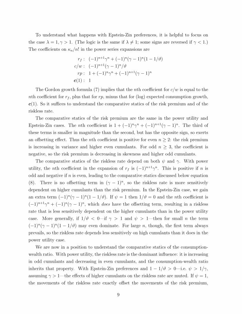
Figure 1a plots the CGF (9) against θ. I choose parameters according to Barro’s

(2006) baseline calibration—γ = 4, σB = 0.02, ρ = 0.03, µ = 0.025, ω = 0.017—and set

b = 0.39 and s = 0.25 to match the mean and variance of the distribution of jumps used

in the same paper. I also plot the CGF that results in the absence of jumps (ω = 0). In

the latter case, I adjust the drift of consumption growth to keep mean log consumption

growth constant; in the figure, this means that the two curves are tangent at the origin.

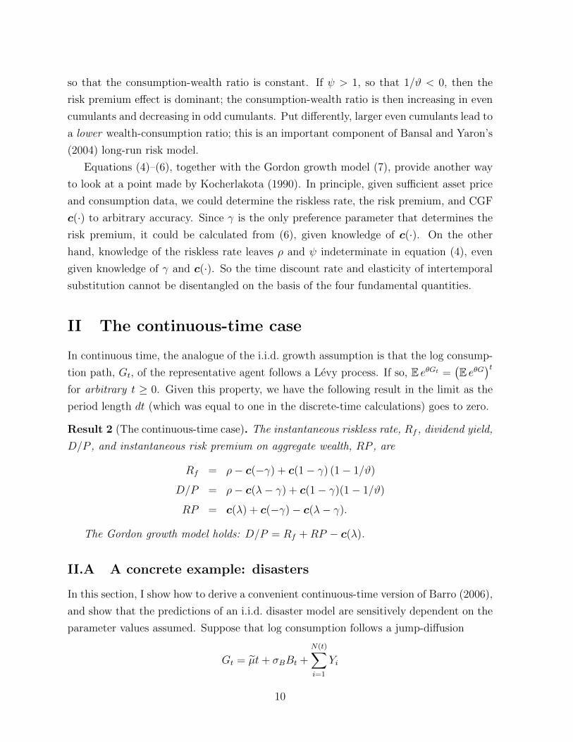
Zooming out on Figure 1a, we obtain Figure 1b, which further illustrates the equity

premium and riskless rate puzzles. With jumps, the CGF is visible at the right-hand

side of the figure; the CGF explodes so quickly as θ declines that it is only visible for θ

greater than about −5. The jump-free lognormal CGF has incredibly low curvature. For

a realistic riskless rate and equity premium, the model requires a risk aversion above 80.

11

r f c�w cH1L-Γ 1-Γ 1-2 -1

Θ

-0.05

Ρ

0.05

0.10

cHΘL

(a) rf , c/w, and c(1) can be read off the CGF

-100 -80 -60 -40 -20Θ

-0.4

-0.3

-0.2

-0.1

0.1

cHΘL

(b) Zooming out

Figure 1: Left: The CGF with (solid) and without (dashed) jumps. The figure assumes

that ρ = 0.03 and γ = 4. Right: Zooming out. Without jumps, we need enormously high

γ to avoid the riskless rate and equity premium puzzles.

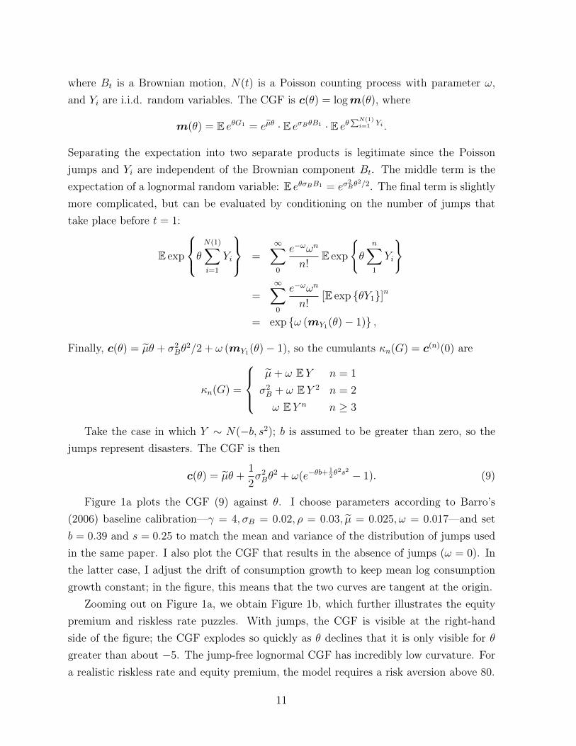
rp�2

-Γ 1-Γ 1-2 -1Θ

0.05

0.1

cHΘL

Figure 2: The risk premium. The figure assumes that γ = 4.

The riskless rate, consumption-wealth ratio and mean consumption growth can be read

directly off the graph, as indicated by the arrows in Figure 1a. The risk premium can be

calculated from these via the Gordon growth formula, or read directly off the graph, as in

Figure 2, by drawing a line from (−γ, c(−γ)) to (1, c(1)) and another from (1−γ, c(1−γ))

to (0, 0). The midpoint of the first line lies above the midpoint of the second by convexity

of the CGF. The risk premium is twice the distance from one midpoint to the other.

The standard lognormal model predicts a counterfactually high riskless rate: in Figure

1a, this is reflected in the fact that the no-jumps CGF lies well below ρ for reasonable

values of θ. Similarly, the standard lognormal model predicts a counterfactually low equity

premium: the no-jump CGF is practically linear over the range [−γ, 1]. Conversely, the

disaster CGF has a shape which allows it to match observed fundamentals closely.

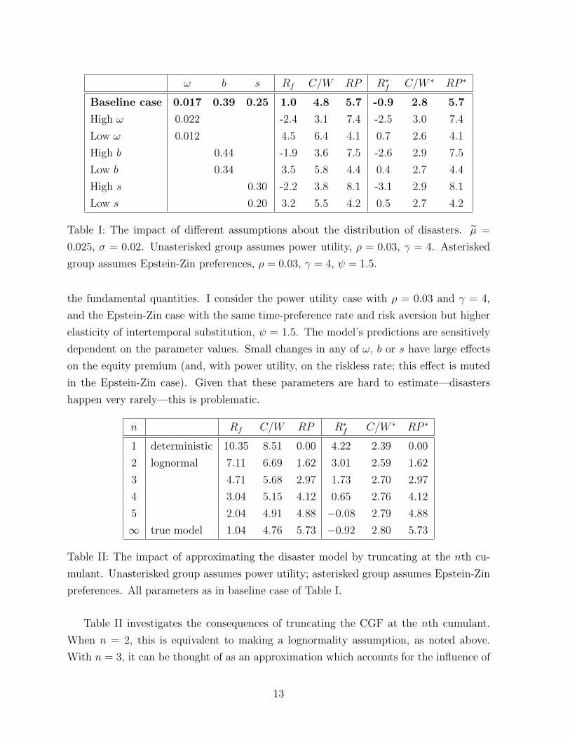
Table I shows how changes in the calibration of the distribution of disasters affect

12

ω b s Rf C/W RP R∗f C/W ∗ RP ∗

Baseline case 0.017 0.39 0.25 1.0 4.8 5.7 -0.9 2.8 5.7

High ω 0.022 -2.4 3.1 7.4 -2.5 3.0 7.4

Low ω 0.012 4.5 6.4 4.1 0.7 2.6 4.1

High b 0.44 -1.9 3.6 7.5 -2.6 2.9 7.5

Low b 0.34 3.5 5.8 4.4 0.4 2.7 4.4

High s 0.30 -2.2 3.8 8.1 -3.1 2.9 8.1

Low s 0.20 3.2 5.5 4.2 0.5 2.7 4.2

Table I: The impact of different assumptions about the distribution of disasters. µ =

0.025, σ = 0.02. Unasterisked group assumes power utility, ρ = 0.03, γ = 4. Asterisked

group assumes Epstein-Zin preferences, ρ = 0.03, γ = 4, ψ = 1.5.

the fundamental quantities. I consider the power utility case with ρ = 0.03 and γ = 4,

and the Epstein-Zin case with the same time-preference rate and risk aversion but higher

elasticity of intertemporal substitution, ψ = 1.5. The model’s predictions are sensitively

dependent on the parameter values. Small changes in any of ω, b or s have large effects

on the equity premium (and, with power utility, on the riskless rate; this effect is muted

in the Epstein-Zin case). Given that these parameters are hard to estimate—disasters

happen very rarely—this is problematic.

n Rf C/W RP R∗f C/W ∗ RP ∗

1 deterministic 10.35 8.51 0.00 4.22 2.39 0.00

2 lognormal 7.11 6.69 1.62 3.01 2.59 1.62

3 4.71 5.68 2.97 1.73 2.70 2.97

4 3.04 5.15 4.12 0.65 2.76 4.12

5 2.04 4.91 4.88 −0.08 2.79 4.88

∞ true model 1.04 4.76 5.73 −0.92 2.80 5.73

Table II: The impact of approximating the disaster model by truncating at the nth cu-

mulant. Unasterisked group assumes power utility; asterisked group assumes Epstein-Zin

preferences. All parameters as in baseline case of Table I.

Table II investigates the consequences of truncating the CGF at the nth cumulant.

When n = 2, this is equivalent to making a lognormality assumption, as noted above.

With n = 3, it can be thought of as an approximation which accounts for the influence of

13

skewness; n = 4 also allows for kurtosis. As is clear from the table, even calculations based

on fourth- or fifth-order approximations do not fully capture the impact of disasters.

II.B A GMM exercise

What would estimates of ρ and γ look like if the baseline disaster model were a literal

description of reality? This section carries out a GMM exercise using the baseline calibra-

tion. I simulate 100 years of annual consumption data, back out asset prices and returns

using the above results, and estimate the parameters ρ and γ from the sample analogues

of the moment conditions

E

[e−ρ(Ct+1

Ct

)−γ(Rt+1 −Rf,t+1)

]= 0 and E

[e−ρ(Ct+1

Ct

)−γ(1 +Rf,t+1)

]= 1.

(10)

These equations apply in the power utility case; the conclusions of this section also apply

in the Epstein-Zin case if ρ is replaced by ρ ≡ ρ + (1 − 1/ϑ) · c(1 − γ). The moment

conditions (10) identify ρ and γ in the model; see the Appendix for a proof.

Explicitly, the estimates ρ and γ are computed by solving

T∑t=1

(Ct+1

Ct

)−γ(Rt+1 −Rf,t+1) = 0

for γ, and using the result to determine ρ from

1

T

T∑t=1

e−ρ(Ct+1

Ct

)−γ(1 +Rf,t+1) = 1.

I show in the supplementary appendix that the standard regularity conditions hold

in this calibration, so that GMM estimates are consistent and asymptotically Normal.

It turns out, though, that 100 years is not enough data for these asymptotic results to

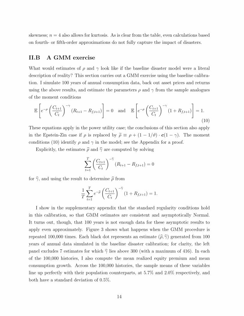
apply even approximately. Figure 3 shows what happens when the GMM procedure is

repeated 100,000 times. Each black dot represents an estimate (ρ, γ) generated from 100

years of annual data simulated in the baseline disaster calibration; for clarity, the left

panel excludes 7 estimates for which γ lies above 300 (with a maximum of 416). In each

of the 100,000 histories, I also compute the mean realized equity premium and mean

consumption growth. Across the 100,000 histories, the sample means of these variables

line up perfectly with their population counterparts, at 5.7% and 2.0% respectively, and

both have a standard deviation of 0.5%.

14

(a) GMM estimates of (ρ, γ) (b) Zooming in

Figure 3: Each of the 100,000 small black dots represents a GMM estimate of (ρ, γ) from

100 years of simulated annual data in the disaster model. The ellipses indicate confidence

regions in which 50% (inner ellipse) and 95% (outer ellipse) of the mass of the distribution

of (ρ, γ) would lie if (ρ, γ) were Normally distributed. Dotted lines in each panel indicate

the model-free parameter restrictions derived in Section III: just 10 of the estimates (ρ, γ)

lie in the lower admissible region, visible in the right-hand panel, in which γ < 1.

The mean estimate (ρ, γ) = (−0.086, 29.5), generated by averaging the resulting

100,000 estimates (ρ, γ), is marked with a green dot. (For comparison, Kocherlakota

(1996) carries out the same exactly identified GMM exercise in real-world data. In my

notation, he estimates ρ = −0.077 and γ = 17.95.) The true value (ρ, γ) = (0.03, 4) is

marked with a red dot. The standard deviation of the estimates ρ is 0.426; the standard

deviation of the estimates γ is 43.5; and the correlation between ρ and γ is −0.42. The

dashed ellipses show confidence regions within which 50% (small ellipse) and 95% (large

ellipse) of the sample points would lie if the data were Normally distributed. Larger esti-

mates of risk aversion tend to be associated with smaller estimates of the time preference

rate: the procedure is struggling to match the data by increasing risk aversion, at the

cost of having to assuming extreme patience in order to match the riskless rate. Finally,

dotted lines indicate model-free parameter restrictions that will be derived in the next

section.

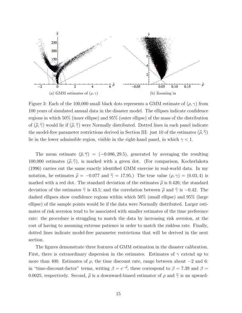
The figures demonstrate three features of GMM estimation in the disaster calibration.

First, there is extraordinary dispersion in the estimates. Estimates of γ extend up to

more than 400. Estimates of ρ, the time discount rate, range between about −2 and 6:

in “time-discount-factor” terms, writing β = e−ρ, these correspond to β = 7.39 and β =

0.0025, respectively. Second, ρ is a downward-biased estimator of ρ and γ is an upward-

15

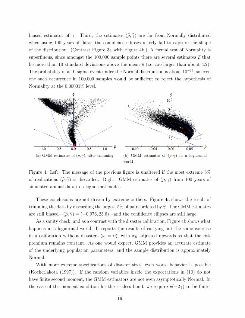
biased estimator of γ. Third, the estimates (ρ, γ) are far from Normally distributed

when using 100 years of data: the confidence ellipses utterly fail to capture the shape

of the distribution. (Contrast Figure 3a with Figure 4b.) A formal test of Normality is

superfluous, since amongst the 100,000 sample points there are several estimates ρ that

lie more than 10 standard deviations above the mean ρ (i.e. are larger than about 4.2).

The probability of a 10-sigma event under the Normal distribution is about 10−23, so even

one such occurrence in 100,000 samples would be sufficient to reject the hypothesis of

Normality at the 0.00001% level.

(a) GMM estimates of (ρ, γ), after trimming (b) GMM estimates of (ρ, γ) in a lognormal

world

Figure 4: Left: The message of the previous figure is unaltered if the most extreme 5%

of realizations (ρ, γ) is discarded. Right: GMM estimates of (ρ, γ) from 100 years of

simulated annual data in a lognormal model.

These conclusions are not driven by extreme outliers: Figure 4a shows the result of

trimming the data by discarding the largest 5% of pairs ordered by γ. The GMM estimates

are still biased—(ρ, γ) = (−0.076, 23.6)—and the confidence ellipses are still large.

As a sanity check, and as a contrast with the disaster calibration, Figure 4b shows what

happens in a lognormal world. It reports the results of carrying out the same exercise

in a calibration without disasters (ω = 0), with σB adjusted upwards so that the risk

premium remains constant. As one would expect, GMM provides an accurate estimate

of the underlying population parameters, and the sample distribution is approximately

Normal.

With more extreme specifications of disaster sizes, even worse behavior is possible

(Kocherlakota (1997)). If the random variables inside the expectations in (10) do not

have finite second moment, the GMM estimators are not even asymptotically Normal. In

the case of the moment condition for the riskless bond, we require c(−2γ) to be finite;

16

in the case of the consumption claim, we require c(2 − 2γ) to be finite. If the former

is finite, the latter is too, so in summary the GMM approach is only valid if c(−2γ) is

finite. This is not assured by the assumptions that ensure finite utility, or a finite consol

price. Below, I construct an example for which the GMM approach fails not only in finite

samples, but even asymptotically: Figure 6b plots the CGF of (an extreme case of) such

a distribution.

III Restrictions on preference parameters

I now assume that the riskless rate, consumption-wealth ratio, and risk premium (and

hence expected consumption growth, via the Gordon growth model (7)) are observable

and take the values given in Table III.4 The observables provide us with information about

the shape of the CGF; this section shows how to use this information to derive restrictions

on the preference parameters that must hold in any Epstein-Zin/i.i.d. model, no matter

what is going on in the tails. The restrictions are of particular interest when there are

small sample biases, as in the previous section, and they continue to be valid when GMM

breaks down entirely, as discussed at the end of the previous section.

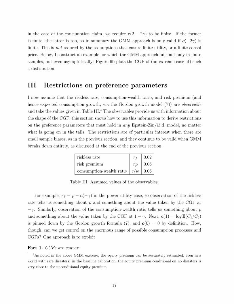
riskless rate rf 0.02

risk premium rp 0.06

consumption-wealth ratio c/w 0.06

Table III: Assumed values of the observables.

For example, rf = ρ − c(−γ) in the power utility case, so observation of the riskless

rate tells us something about ρ and something about the value taken by the CGF at

−γ. Similarly, observation of the consumption-wealth ratio tells us something about ρ

and something about the value taken by the CGF at 1 − γ. Next, c(1) = logE(C1/C0)

is pinned down by the Gordon growth formula (7), and c(0) = 0 by definition. How,

though, can we get control on the enormous range of possible consumption processes and

CGFs? One approach is to exploit

Fact 1. CGFs are convex.

4As noted in the above GMM exercise, the equity premium can be accurately estimated, even in a

world with rare disasters: in the baseline calibration, the equity premium conditional on no disasters is

very close to the unconditional equity premium.

17

Proof. Since c(θ) = logm(θ), we have

c′′(θ) =m(θ) ·m′′(θ)−m′(θ)2

m(θ)2

=E eθG EG2eθG −

(EGeθG

)2m(θ)2

.

The numerator of this expression is positive by a version of the Cauchy-Schwartz inequality

which states that EX2 ·EY 2 ≥ E(|XY |)2 for any random variables X and Y . In this case,

we need to set X = eθG/2 and Y = GeθG/2. (See Billingsley (1995), for further discussion

of this and other properties of CGFs.)

This fact can be used to derive sharp preference parameter bounds based on observ-

ables.

Result 3. In the power utility case, we have

rf − c/w ≤c/w − ργ − 1

≤ rp+ rf − c/w. (11)

In the Epstein-Zin case, we have

rf − c/w ≤c/w − ρ1/ψ − 1

≤ rp+ rf − c/w. (12)

Moreover, these bounds are sharp: for any ε > 0 there are distributions of consumption

growth, and parameter choices for ρ, γ and ψ, that are consistent with the observables and

satisfy c/w−ρ1/ψ−1 < rf−c/w+ε; and other distributions of consumption growth and parameter

choices that are consistent with the observables and satisfy c/w−ρ1/ψ−1 > rp+ rf − c/w − ε.

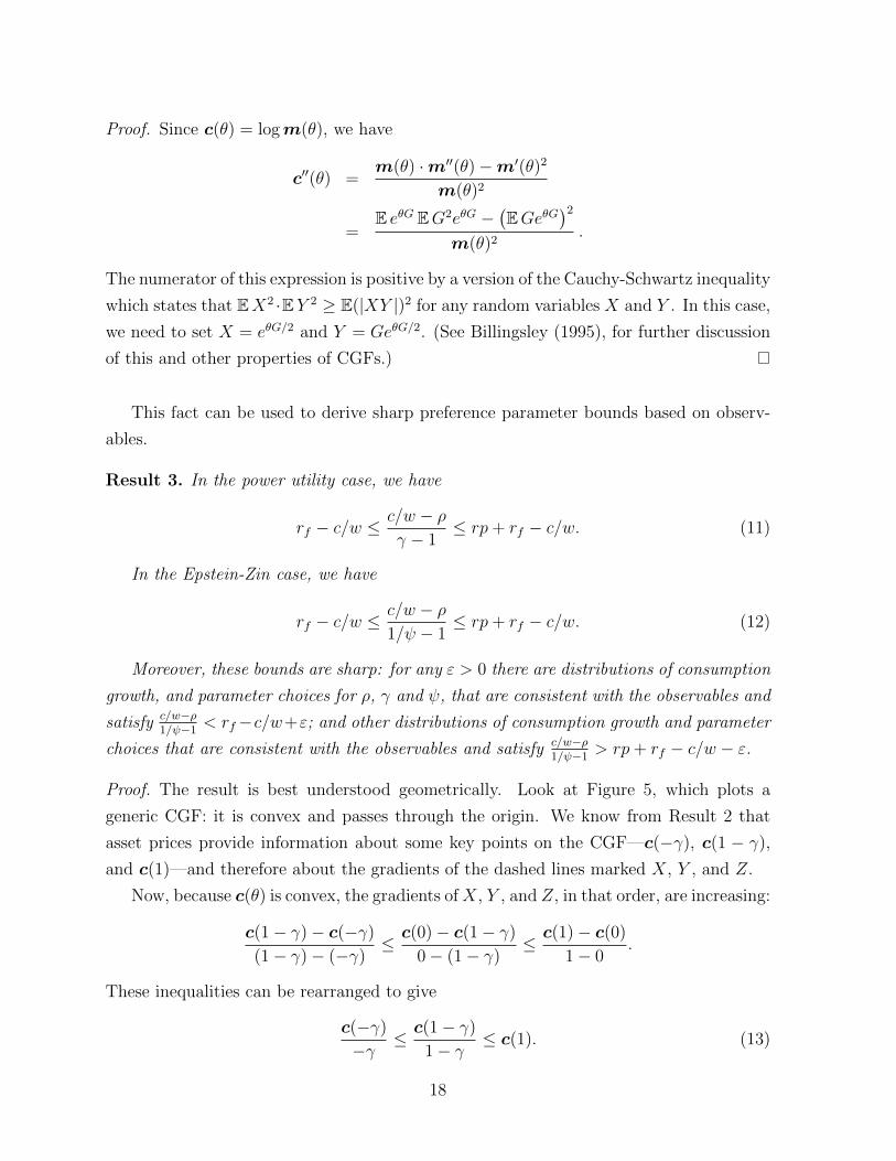
Proof. The result is best understood geometrically. Look at Figure 5, which plots a

generic CGF: it is convex and passes through the origin. We know from Result 2 that

asset prices provide information about some key points on the CGF—c(−γ), c(1 − γ),

and c(1)—and therefore about the gradients of the dashed lines marked X, Y , and Z.

Now, because c(θ) is convex, the gradients ofX, Y , and Z, in that order, are increasing:

c(1− γ)− c(−γ)

(1− γ)− (−γ)≤ c(0)− c(1− γ)

0− (1− γ)≤ c(1)− c(0)

1− 0.

These inequalities can be rearranged to give

c(−γ)

−γ≤ c(1− γ)

1− γ≤ c(1). (13)

18

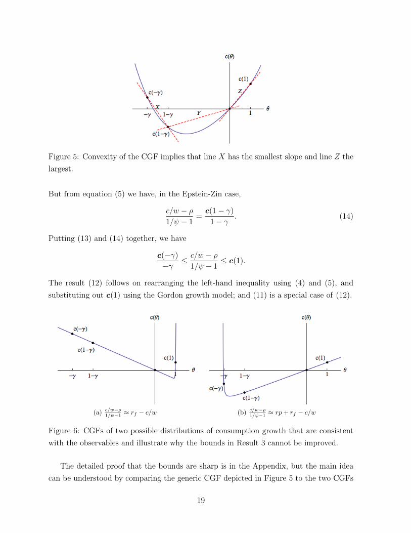
Figure 5: Convexity of the CGF implies that line X has the smallest slope and line Z the

largest.

But from equation (5) we have, in the Epstein-Zin case,

c/w − ρ1/ψ − 1

=c(1− γ)

1− γ. (14)

Putting (13) and (14) together, we have

c(−γ)

−γ≤ c/w − ρ

1/ψ − 1≤ c(1).

The result (12) follows on rearranging the left-hand inequality using (4) and (5), and

substituting out c(1) using the Gordon growth model; and (11) is a special case of (12).

(a) c/w−ρ1/ψ−1 ≈ rf − c/w (b) c/w−ρ

1/ψ−1 ≈ rp+ rf − c/w

Figure 6: CGFs of two possible distributions of consumption growth that are consistent

with the observables and illustrate why the bounds in Result 3 cannot be improved.

The detailed proof that the bounds are sharp is in the Appendix, but the main idea

can be understood by comparing the generic CGF depicted in Figure 5 to the two CGFs

19

shown in Figure 6, which indicate how the two extremes can be approximately attained.

The Appendix demonstrates that there are distributions of consumption growth whose

CGFs look like those in Figure 6—i.e., have the properties that (i) they are almost linear

on the intervals [−γ, 0] in the case represented by Figure 6a, or on [1 − γ, 1] in the case

represented by Figure 6b; and (ii) they are consistent with the observables, which pins

down c(1) and the gap c(1− γ)− c(−γ).

The intuition is that as ψ approaches one, the consumption-wealth ratio approaches

ρ. Therefore, if the consumption-wealth ratio is to be far from ρ, ψ must be far from

one. Result 3 turns this qualitative statement into a quantitative one, without making

assumptions about what is going on in the tails. Using the values rp = 6%, rf = 2%, c/w =

6%, we have the restriction that −0.04 ≤ (0.06− ρ)/(1/ψ − 1) ≤ 0.02. The shaded areas

in Figure 7 illustrate where the parameters must lie. If ψ > 1, then ρ is constrained to lie

between 0.02 and 0.08; if also ψ < 2, then ρ must lie between 0.04 and 0.07. If γ = 1 in

the power utility case, or if ψ = 1 in the Epstein-Zin case, then ρ is exactly identified by

the consumption-wealth ratio.

0.00 0.02 0.04 0.06 0.08 0.10Ρ

1

2

3

4Γ

(a) Power utility case: γ and ρ

0.00 0.02 0.04 0.06 0.08 0.10Ρ

0.5

1.0

1.5

2.0Ψ

(b) Epstein-Zin case: ψ and ρ

Figure 7: Parameter restrictions for i.i.d. models with rp = 6%, rf = 2% and c/w = 6%.

To the extent that Dt = Cλt is a reasonable approximation of leverage, we can say

even more. For, we observe the consumption-wealth ratio c/w, wealth risk premium rpw

and the dividend yield on the market d/p and market risk premium rpm (that is, observe

(4)–(6), together with the expressions that result on substituting in λ = 1). The following

relationships hold:

c/w − d/p = c(λ− γ)− c(1− γ)

ϑ(ρ− c/w) + c/w − d/p = c(λ− γ)

rpm + rf − d/p = c(λ)

20

By convexity, we have

c(λ− γ)− c(1− γ)

λ− 1≤ c(λ− γ)

λ− γ≤ c(λ)

λ.

Substituting in, we have joint bounds on ρ, γ and ψ:

c/w − d/pλ− 1

≤ ϑ(ρ− c/w) + c/w − d/pλ− γ

≤ rpm + rf − d/pλ

.

III.A Hansen-Jagannathan and good-deal bounds

Hansen and Jagannathan (1991) derived a bound that relates the standard deviation and

mean of the stochastic discount factor, M , to the Sharpe ratio on an arbitrary asset, SR:

SR ≤ σ(M)

EM. (15)

In the Epstein-Zin-i.i.d. setting, the right-hand side of (15) becomes

σ(M)

EM=

√EM2

(EM)2− 1

=√ec(−2γ)−2c(−γ) − 1. (16)

Combining (15) and (16), we obtain the Hansen-Jagannathan bound in CGF notation:

log(1 + SR2

)≤ c(−2γ)− 2c(−γ) . (17)

Cochrane and Saa-Requejo (2000) observe that inequality (15) suggests a natural way

to restrict asset-pricing models. Suppose σ(M)/EM ≤ h; then (15) implies that the

maximal Sharpe ratio is less than h. In CGF notation, the good-deal bound is written

c(−2γ)− 2c(−γ) ≤ log(1 + h2

). (18)

Suppose, for example, that we wish to impose the restriction that Sharpe ratios above

1 are too good a deal to be available. Then the good-deal bound is c(−2γ) − 2c(−γ) ≤log 2. This expression can be evaluated under particular parametric assumptions about

the consumption process. In the case in which consumption growth is lognormal, with

volatility of log consumption equal to σ, it supplies an upper bound on risk aversion:

γ ≤√

log 2/σ (which is about 42 if σ = 0.02). However, this upper bound is rather weak,

and in any case the postulated consumption process is inconsistent with observed features

of asset markets such as the high equity premium and low riskless rate. Alternatively, one

21

might model the consumption process as subject to disasters in the sense of Section II.A.

In this case, the good-deal bound implies tighter restrictions on γ, but these restrictions

are sensitively dependent on the disaster parameters.

In order to progress from (18) to a bound on γ and ρ which does not require parametriza-

tion of the consumption process, we want to relate c(−2γ)− 2c(−γ) to quantities which

can be directly observed. For example, the Hansen-Jagannathan bound (17) improves on

a conclusion which follows from the convexity of the CGF, namely, that

0 ≤ c(−2γ)− 2c(−γ) . (19)

This trivial inequality follows by considering the value of the CGF at the three points

c(0), c(−γ), and c(−2γ). Convexity implies that the average slope of the CGF is more

negative (or less positive) between −2γ and −γ than it is between −γ and 0:

c(−γ)− c(−2γ)

γ≤ c(0)− c(−γ)

γ.

Equation (19) follows immediately, given that c(0) = 0. Combining (18) and (19), we

obtain the (underwhelming!) result that 0 ≤ log (1 + h2).

However, we can sharpen (19) by comparing the slope of the CGF between −2γ and

−γ to the slope between −γ and 1− γ (rather than between −γ and 0):

c(−γ)− c(−2γ)

γ≤ c(1− γ)− c(−γ)

1.

This implies, by Result 1, that c(−2γ)− 2c(−γ) ≥ (γ − 1)(c/w − rf ) + ϑ(c/w − ρ), and

hence

Result 4. If the maximal Sharpe ratio is less than or equal to h, then we must have

(γ − 1)(c/w − rf ) + ϑ(c/w − ρ) ≤ log(1 + h2

). (20)

The important feature of this result is that by exploiting the observable consumption-

wealth ratio and riskless rate, we do not need to take a stand on what is going on in the

tails.

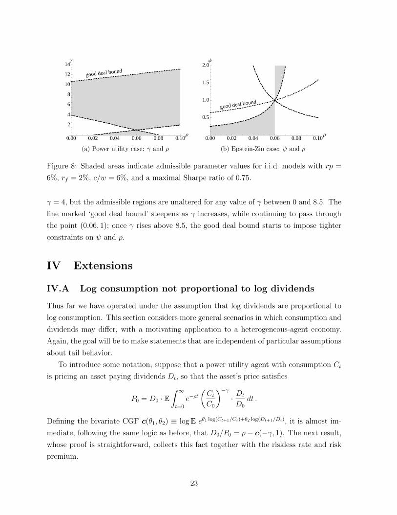
Figure 8 reproduces the bounds of Figure 7, adding in the good deal bound (20) with

h = 0.75, i.e. ruling out Sharpe ratios above 0.75. Shaded areas indicate admissible

parameter values. In the right-hand panel, admissible values lie below the line marked

‘good deal bound’ when ψ < 1 and above it when ψ > 1. There are also admissible values

of ρ and ψ not visible in the figure, with ρ large and ψ close to zero. The figure assumes

22

good deal bound

0.00 0.02 0.04 0.06 0.08 0.10Ρ

2

4

6

8

10

12

14Γ

(a) Power utility case: γ and ρ

good deal bound

0.00 0.02 0.04 0.06 0.08 0.10Ρ

0.5

1.0

1.5

2.0Ψ

(b) Epstein-Zin case: ψ and ρ

Figure 8: Shaded areas indicate admissible parameter values for i.i.d. models with rp =

6%, rf = 2%, c/w = 6%, and a maximal Sharpe ratio of 0.75.

γ = 4, but the admissible regions are unaltered for any value of γ between 0 and 8.5. The

line marked ‘good deal bound’ steepens as γ increases, while continuing to pass through

the point (0.06, 1); once γ rises above 8.5, the good deal bound starts to impose tighter

constraints on ψ and ρ.

IV Extensions

IV.A Log consumption not proportional to log dividends

Thus far we have operated under the assumption that log dividends are proportional to

log consumption. This section considers more general scenarios in which consumption and

dividends may differ, with a motivating application to a heterogeneous-agent economy.

Again, the goal will be to make statements that are independent of particular assumptions

about tail behavior.

To introduce some notation, suppose that a power utility agent with consumption Ct

is pricing an asset paying dividends Dt, so that the asset’s price satisfies

P0 = D0 · E∫ ∞t=0

e−ρt(CtC0

)−γ· Dt

D0

dt .

Defining the bivariate CGF c(θ1, θ2) ≡ logE eθ1 log(Ct+1/Ct)+θ2 log(Dt+1/Dt), it is almost im-

mediate, following the same logic as before, that D0/P0 = ρ− c(−γ, 1). The next result,

whose proof is straightforward, collects this fact together with the riskless rate and risk

premium.

23

Result 5. If consumption growth Gt ≡ logCt/C0 and dividend growth Ht ≡ logDt/D0

are distinct, potentially correlated, Levy processes, then

D0/P0 = ρ− c(−γ, 1)

Rf = ρ− c(−γ, 0)

RP = c(0, 1) + c(−γ, 0)− c(−γ, 1).

Constantinides and Duffie (1996) have shown that accounting for heterogeneity may

contribute to an understanding of the equity premium puzzle. On the other hand, Gross-

man and Shiller (1982) have shown that if agents’ consumption processes follow diffusions,

risk premia are unaffected by heterogeneity. The tension between these two results will be

resolved by showing that heterogeneity matters to the extent that it is present at times of

aggregate jumps. The presence of jumps lends a discrete-time flavor to the model, and as

a result it lies closer on the spectrum to Constantinides-Duffie than to Grossman-Shiller.

I assume that agents suffer idiosyncratic shocks to consumption, perhaps because

agents have labor income risk which is uninsurable for moral hazard reasons.5 All agents

have power utility. Agent i’s log consumption process is given by

logCi,tCi,0

= µt+ σBt +Nt∑j=1

Yj︸ ︷︷ ︸common to all agents

+σ1Bit −1

2σ21t︸ ︷︷ ︸

type (i)

+

Ni,t∑j=1

Xi,j︸ ︷︷ ︸type (ii)

+Nt∑j=1

Yi,j︸ ︷︷ ︸type (iii)

(21)

Here Bt is a Brownian motion, and Yj are the i.i.d. sizes of jumps, which occur at times

dictated by the Poisson process Nt, with arrival rate ω; these shocks are common to

all agents. I assume that the jumps are bad—or at least, not good—news on average,

so E eYj ≤ 1. There are also three types of idiosyncratic shocks: (i) an idiosyncratic

Brownian motion component, Bi,t; (ii) jumps whose size Xi,k and timing (determined by

the Poisson process Ni,t) are idiosyncratic; and (iii) jumps of idiosyncratic size Yi,k, whose

timing coincides with aggregate disasters, to capture the fact that disasters do not have

the same impact on all agents. I assume that Xi,j and Yk,l are i.i.d. across i, j, k and l,

and Ni,t are Poisson processes, independent across i, with arrival rate ω2. Finally, σ1 and

ω2 are constant across all agents i.

Aggregate quantities are computed by summing over agents i; I assume that a law of

large numbers holds so that this process is equivalent to taking an expectation over i. With

5Storesletten, Telmer and Yaron (2004) show that idiosyncratic shocks are highly persistent, and large,

with a standard deviation of about 0.25.

24

this assumption, together with the normalization that for all i and k, E eXi,k = E eYi,k = 1,

(21) implies that aggregate consumption evolves according to log Ct

C0= µt+σBt+

∑Nt

j=1 Yj.

The upshot is that all agents attach the same value to the “equity” claim to aggregate

consumption, so as in Constantinides and Duffie (1996) there is a no-trade equilibrium in

which agent i consumes Ci,t at time t. The Euler equation holds for each agent i, so the

price of equity, P , must satisfy

P = E∫ ∞0

e−ρt(Ci,tCi,0

)−γ· Ct dt . (22)

Result 5 now applies with Gt = logCit/Ci0 and Ht = logCt/C0. Defining mD(θ) ≡ E eθYj ,m2(θ) ≡ E eθXi,k , and m3(θ) ≡ E eθYi,j , the CGF of (G1, H1) is c(θ1, θ2) = µ (θ1 + θ2) +12σ2 (θ1 + θ2)

2 + 12σ21θ1(θ1 − 1) + ω2 [m2(θ1)− 1] + ω [mD (θ1 + θ2)m3 (θ1)− 1]. The divi-

dend yield, riskless rate, and risk premium follow from Result 5.

A naive econometrician who uses aggregate consumption in calculations of these fun-

damentals is wrongly dropping the is in (22), i.e. replacing Gt in the CGF by Ht, or

equivalently using the function c(0, θ1 + θ2) in place of c(θ1, θ2). The discrepancies be-

tween the true values and incorrect predictions based on aggregate quantities (denoted

by bars) are

D/P −D/P = −σ21γ(γ + 1)/2− ω2 [m2(−γ)− 1]− ωmD(1− γ) [m3(−γ)− 1](23)

Rf −Rf = −σ21γ(γ + 1)/2− ω2 [m2(−γ)− 1]− ωmD(−γ) [m3(−γ)− 1] (24)

RP −RP = ω [mD(−γ)−mD(1− γ)] [m3(−γ)− 1] . (25)

All three types of heterogeneity influence the dividend yield and riskless rate. But

if there are no aggregate disasters—ω = 0—then heterogeneity has no effect on the risk

premium, as in Grossman and Shiller (1982). Even if there are disasters, heterogeneity of

type (i) or type (ii) has no effect on risk premia, as in Krueger and Lustig (2010). Using

these expressions, we can sign the effects of heterogeneity no matter what the distribution

of jumps.

Result 6 (Robust implications of heterogeneity). Heterogeneity drives down the dividend

yield and riskless rate, and increases the risk premium: D/P ≤ D/P ; Rf ≤ Rf ; and

RP ≥ RP .

Campbell (2003) and Cochrane (2008) have argued, based on calculations in lognormal

or approximately lognormal models, that heterogeneity is unlikely to be quantitatively

relevant for the equity premium puzzle. The good news is that (25) shows that this

25

conclusion is altered—heterogeneity may be quantitatively important—in the presence of

jumps. Suppose that aggregate and idiosyncratic type (iii) jumps in log consumption are

Normally distributed, Yj ∼ N(−b, s2) and Yi,k ∼ N(−s2i /2, s2i ). Then mD(θ) = e−bθ+s2θ2/2

and m3(θ) = es2i θ(θ−1)/2. From (25), this increases the equity premium by

ω(ebγ+s

2γ2/2 − eb(γ−1)+s2(γ−1)2/2)(

es2i γ(γ+1)/2 − 1

).

This increases extremely rapidly in γ: relative to the baseline calibration, si = 0.25 causes

the equity premium to increase by an extra 528bp if γ = 4, and by 1982bp if γ = 5.

But here too, disasters are a double-edged sword. The bad news is that heterogeneity

only matters for risk premia to the extent that it is present at times of aggregate disaster.

This is frustrating from the point of view of empirical work, since it means that the con-

siderable amount of information about heterogeneity in “normal” times that is available

in individual-level datasets is irrelevant for risk premia. Thus the difficulties in identifying

parameters discussed in previous sections extend to the heterogeneous agent case. This

may explain why several authors have failed to find empirical evidence that heterogeneity

matters. For example, Heaton and Lucas (1996) and Lettau (2002) do not consider the

relevance of disasters. Cogley (2002) does, but truncates at the third moment; moreover

his data only run from 1980, so do not contain any examples of disasters in Barro’s (2006)

sense.

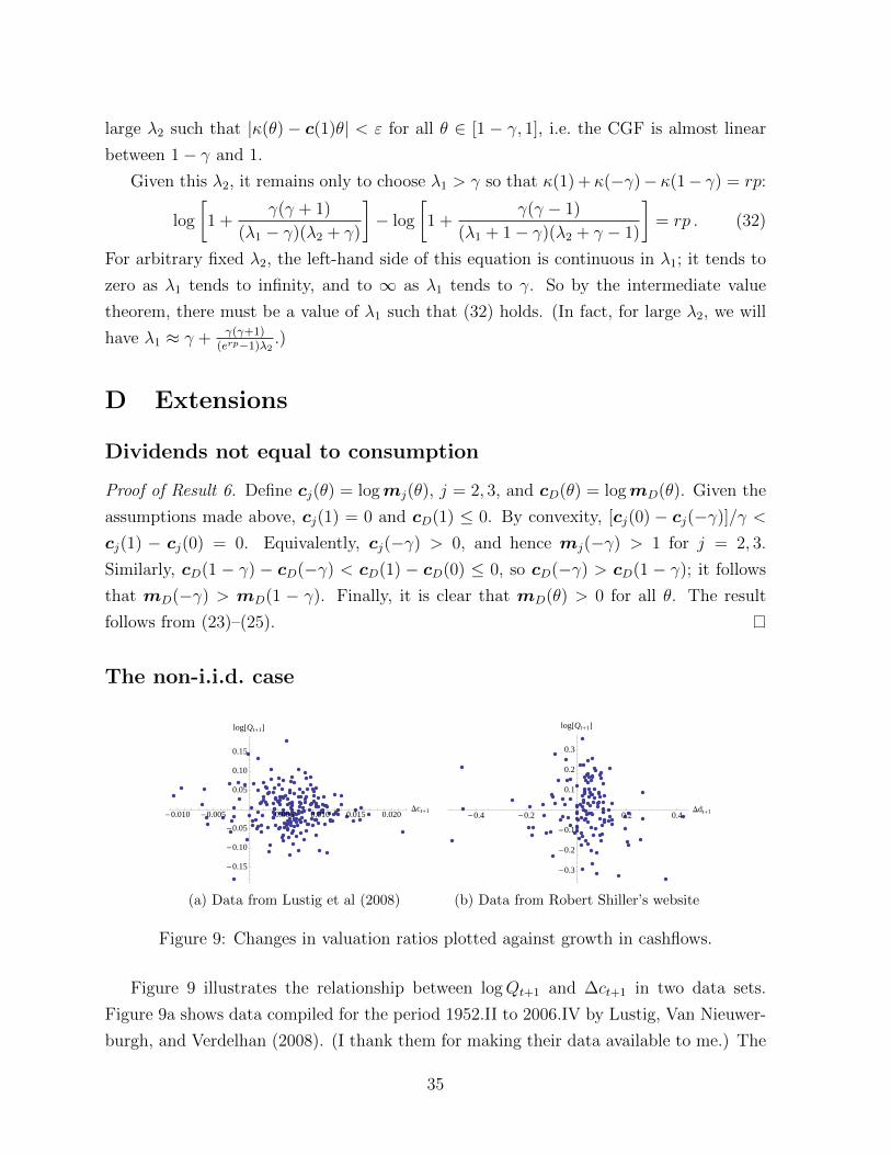
IV.B Non-i.i.d. consumption growth

An extensive literature has documented that time variation in valuations contributes

a sizeable proportion of equity volatility. To capture this feature while still allowing for

arbitrarily distributed consumption growth, I now drop the assumption that consumption

growth is i.i.d. Valuations are then time-varying, so that we have nontrivial valuation

shocks Qt+1:

1 +Wt+1

Ct+1

=

(1 +

Wt

Ct

)Qt+1. (26)

In the i.i.d. case, valuation ratios were constant and Qt+1 ≡ 1. I now assume only that

EtQt+1 = 1. The joint behavior of consumption growth and valuation ratios can be sum-

marized by the conditional CGF ct(θ1, θ2) = logEt exp {θ1 log(Ct+1/Ct) + θ2 logQt+1}.An Epstein-Zin investor’s Euler equation implies that

Wt

Ct= Et

[e−ρϑ

(Ct+1

Ct

)−ϑ/ψ(1 +Rm,t+1)

ϑ−1(Ct+1 +Wt+1

Ct

)]. (27)

26

Using (26), we have

1 +Rm,t+1 =

(1 +

CtWt

)Ct+1

CtQt+1 , (28)

so the expected return moves around with the valuation ratio Ct/Wt. We also have

Ct+1 +Wt+1

Ct=Wt

Ct

(1 +

CtWt

)Ct+1

CtQt+1 . (29)

Substituting (28) and (29) into (27) and rearranging, we find that

1 +CtWt

= exp {ρ− ct(1− γ, ϑ)/ϑ} .

Using this together with (28), Et(1 +Rm,t+1) = exp {ρ+ ct(1, 1)− ct(1− γ, ϑ)/ϑ}. Simi-

larly, the price of a one-period bond, Bt, is

Bt = Et

[e−ρϑ

(Ct+1

Ct

)−ϑ/ψ(1 +Rm,t+1)

ϑ−1

]= exp {−ρ+ (1/ϑ− 1)ct(1− γ, ϑ) + ct(−γ, ϑ− 1)} .

Now define, in line with previous notation, the consumption-wealth ratio c/wt ≡ log(1 +

Ct/Wt), riskless rate rf,t ≡ − logBt, and risk premium rpt ≡ logEt(1 +Rm,t+1)− rf,t; we

have

c/wt = ρ− ct(1− γ, ϑ)/ϑ

rf,t = ρ+ (1− 1/ϑ)ct(1− γ, ϑ)− ct(−γ, ϑ− 1)

rpt = ct(1, 1) + ct(−γ, ϑ− 1)− ct(1− γ, ϑ).

As before, the fundamentals provide information about the values taken at various

points by the CGF, and as before, the CGF is a convex function. Now, however, because

the points (1, 1), (1 − γ, ϑ), and (−γ, ϑ − 1) do not lie on a line, there are no direct

constraints imposed by convexity in the general case.6 However, I show in the appendix

that the hypothesis that Qt+1 and Ct+1/Ct are independent of one another cannot be

rejected in the data. If we assume that they are indeed independent then the analysis

simplifies nicely,7 and the previous results can be extended—perfectly, in the power utility

case—to the case of non-i.i.d. consumption growth.

6Except in the limiting case ψ = ∞; then, the points do lie on a line and without any further

assumptions the convexity argument goes through. Equation (12) holds, and hence rf,t ≤ ρ ≤ rf,t + rpt.7Even if aggregate consumption growth is independent of Qt+1, the consumption growth of marginal

investors may be an important determinant of valuation ratios. In the supplementary appendix, I il-

lustrate this possibility with an equilibrium model and show how the methodology of the paper can be

adapted to it.

27

Result 7. With power utility, Results 3 and 4 continue to hold, with fundamentals replaced

by conditional fundamentals. With Epstein-Zin preferences, the right-hand inequality in

(12) holds in the region ψ ≥ 1/γ, and the left-hand inequality holds in the region ψ ≤min {1/γ, 2/(1 + γ)}; and Result 4 holds if ϑ < 0 or ϑ > 2.

V Conclusion

As pointed out by Rietz (1988), Barro (2006) and Weitzman (2007), the tails of the

distribution of consumption growth exert an enormous influence on asset prices. This

paper takes an agnostic approach regarding the existence and importance of disasters,

and introduces a framework that handles general i.i.d. consumption growth processes.

The framework leads to simple and intuitive formulas that shed light on the impact of the

higher cumulants of consumption growth on the riskless rate, consumption-wealth ratio

and risk premium.

The framework is flexible: in a heterogeneous-agent example, I show that consumption

heterogeneity gives a huge extra kick to the disaster logic if it is present at times of disaster,

and I show how the parameter bounds derived under the i.i.d. assumption can be extended

to the case with non-i.i.d. consumption growth and time-varying valuation ratios, under

an independence assumption that cannot be rejected in the data.

Disasters are a double-edged sword. They exert an enormous influence on asset prices,

and hence provide a potential explanation for the equity premium puzzle (good); but

the predictions of disaster models are sensitively dependent on the assumptions made

about the hard-to-estimate parameters governing the size and frequency of disasters (bad).

A central theme of this paper is that we can sidestep this discouraging observation by

exploiting a simple but powerful fact: CGFs are always convex. This convexity imposes

constraints that hold no matter what is going on in the tails—even in economies in which

the distribution of disasters is so severe that GMM is invalid even asymptotically.

VI References

Abel, A. B., 1999, Risk Premia and Term Premia in General Equilibrium, Journal of Monetary

Economics, 43:3–33.

Abel, A. B., 2008, Equity Premia with Benchmark Levels of Consumption: Closed-Form Results, in

R. Mehra, Ed., Handbook of the Equity Risk Premium, Elsevier.

28

Aıt-Sahalia, Y., Cacho-Diaz, J. and T. R. Hurd, 2006, Portfolio Choice with Jumps: A Closed Form

Solution, preprint.

Backus, D. K., Chernov, M. and I. W. R. Martin, 2011, Disasters Implied by Equity Index Options,

Journal of Finance, 66:6:1969–2012.

Backus, D. K., Foresi, S. and C. I. Telmer, 2001, Affine Term Structure Models and the Forward

Premium Anomaly, Journal of Finance, 56:1:279–304.

Barro, R. J., 2006, Rare Disasters and Asset Markets in the Twentieth Century, Quarterly Journal

of Economics, 121:3:823–866.

Barro, R. J., 2009, Rare Disasters, Asset Prices, and Welfare Costs, American Economic Review,

99:1:243–264.

Bonomo, M., and R. Garcia, 1996, Consumption and Equilibrium Asset Prices: An Empirical As-

sessment, Journal of Empirical Finance, 3:239–265.

Bonomo, M., R. Garcia, N. Meddahi and R. Tedongap, 2009, Disappointment Aversion, Long-Run

Risks, and Aggregate Asset Prices, preprint.

Billingsley, P., 1995, Probability and Measure, 3rd edition (John Wiley & Sons, New York, NY).

Blum, J. R., J. Kiefer, and M. Rosenblatt, 1961, Distribution Free Tests of Independence Based on

the Sample Distribution Function, Annals of Mathematical Statistics, 32:485–498.

Brockett, P. L., and Y. Kahane, 1992, Risk, Return, Skewness and Preference, Management Science,

38:6:851–866.

Campbell, J. Y., 1986, Bond and Stock Returns in a Simple Exchange Model, Quarterly Journal of

Economics, 101:4:785–804.

Campbell, J. Y., 2003, Consumption-Based Asset Pricing, Chapter 13 in George Constantinides,

Milton Harris and Rene Stulz eds., Handbook of the Economics of Finance vol. IB (North-

Holland, Amsterdam), 803–887.

Carr, P. and D. Madan, 1998, Option Valuation Using the Fast Fourier Transform, Journal of Com-

putational Finance, 2:61–73.

Cecchetti, S. G., P. Lam, and N. C. Mark, 1993, The Equity Premium and the Risk-Free Rate:

Matching the Moments, Journal of Monetary Economics, 31:21–45.

Cochrane, J. H., 2008, Financial Markets and the Real Economy, in Rajnish Mehra, Ed. Handbook

of the Equity Premium, Elsevier.

Cochrane, J. H. and J. Saa-Requejo, 2000, Beyond Arbitrage: Good Deal Asset Price Bounds in

Incomplete Markets, Journal of Political Economy, 108:1:79–119.

Cogley, T., 1990, International Evidence on the Size of the Random Walk in Output, Journal of

Political Economy, 98:3:501–518.

Cogley, T., 2002, Idiosyncratic Risk and the Equity Premium: Evidence from the Consumer Expen-

diture Survey, Journal of Monetary Economics, 49:309–334.

Constantinides, G. M. and D. Duffie, 1996, Asset Pricing with Heterogeneous Consumers, Journal

29

of Political Economy, 104:2:219–240.

Cont, R. and P. Tankov, 2004, Financial Modelling with Jump Processes (Chapman & Hall/CRC,

FL).

Cvitanic, J., Polimenis, V. and F. Zapatero, 2005, Optimal Portfolio Allocation with Higher Moments,

preprint.

Epstein, L., and S. Zin, 1989, Substitution, Risk Aversion, and the Temporal Behavior of Consump-

tion and Asset Returns: A Theoretical Framework, Econometrica, 57:937–969.

Eraker, B., 2008, Affine General Equilibrium Models, Management Science, 54:2068–2080.

Gabaix, X., 2009, Linearity-Generating Processes: A Modelling Tool Yielding Closed Forms for Asset

Prices, preprint.

Garcia, R., R. Luger, and E. Renault, 2003, Empirical Assessment of an Intertemporal Option Pricing

Model with Latent Variables, Journal of Econometrics, 116:49–83.

Garcia, R., N. Meddahi and R. Tedongap, 2009, Disappointment Aversion, Long-Run Risks and

Aggregate Asset Prices, preprint.

Grossman, S. J. and R. J. Shiller, 1982, Consumption Correlatedness and Risk Measurement in

Economies with Non-Traded Assets and Heterogeneous Information, Journal of Financial Eco-

nomics 10:195–210.

Hansen, L. P., 1982, Large Sample Properties of Generalized Method of Moments Estimators, Econo-

metrica, 50:4:1029–1059.

Hansen, L. P. and R. Jagannathan, 1991, Implications of Security Market Data for Models of Dynamic

Economies, Journal of Political Economy, 99:2:225–262.

Hansen, L. P., and K. J. Singleton, 1982, Generalized Instrumental Variables Estimation of Nonlinear

Rational Expectations Models, Econometrica, 50:5:1269–1286.

Heaton, J., and D. J. Lucas, Evaluating the Effects of Incomplete Markets on Risk Sharing and Asset

Pricing, Journal of Political Economy, 104:3:443–487.

Hoeffding, W., 1948, A Non-Parametric Test of Independence, Annals of Mathematical Statistics,

19:4:546–557.

Hollander, M., and D. A. Wolfe, 1999, Nonparametric Statistical Methods, 2nd edition (Wiley, NY).

Hong, Y., 1996, Testing for Independence Between Two Covariance Stationary Time Series, Biometrika,

83:3:615–625.

Julliard, C. and A. Ghosh, 2008, Can Rare Events Explain the Equity Premium Puzzle?, preprint.

Jurek, J. W., 2008, Crash-Neutral Currency Carry Trades, preprint.

Kocherlakota, N. R., 1990, Disentangling the Coefficient of Relative Risk Aversion from the Elasticity

of Intertemporal Substitution: An Irrelevance Result, Journal of Finance, 45:1:175–190.

Kocherlakota, N. R., 1996, The Equity Premium: It’s Still a Puzzle, Journal of Economic Literature,

34:1:42–71.

Kocherlakota, N. R., 1997, Testing the Consumption CAPM with Heavy-Tailed Pricing Errors,

30

Macroeconomic Dynamics, 1:551–567.

Kraus, A., and R. H. Litzenberger, 1976, Skewness Preference and the Valuation of Risk Assets,

Journal of Finance, 31:4:1085–1100.

Krueger, D., and H. Lustig, 2010, When is Market Incompleteness Irrelevant for the Price of Aggre-

gate Risk (and When is it Not)?, Journal of Economic Theory, 145:1–41.

Lettau, M., 2002, Idiosyncratic Risk and Volatility Bounds, or Can Models with Idiosyncratic Risk

Solve the Equity Premium Puzzle?, Review of Economics and Statistics, 84:2:376–380.

Longstaff, F. A, and M. Piazzesi, 2004, Corporate Earnings and the Equity Premium, Journal of

Financial Economics, 74:401–421.

Lustig, H., Van Nieuwerburgh, S. and A. Verdelhan, 2008, The Wealth-Consumption Ratio, working

paper.

Martin, I. W. R., 2011a, The Lucas Orchard, preprint.

Martin, I. W. R., 2011b, The Forward Premium Puzzle in a Two-Country World, preprint.

Rietz, T. A., 1988, The Equity Premium: A Solution, Journal of Monetary Economics, 22:117–131.

Storesletten, K., C. I. Telmer, and A. Yaron, 2004, Cyclical Dynamics in Idiosyncratic Labor Market

Risk, Journal of Political Economy, 112:3:695–717.

Weitzman, M. L., 2007, Subjective Expectations and Asset-Return Puzzles, American Economic

Review, 97:4:1102–1130.

A Proof of Result 1

The Epstein-Zin first-order condition leads to the pricing formula

P = E∞∑1

e−ρϑt(CtC0

)−ϑ/ψ(1 +Rm,0→t)

ϑ−1 (Ct)λ ,

where ϑ = (1− γ)/(1− 1/ψ) and Rm,0→t is the cumulative return on the wealth portfolio

from period 0 to period t. I assume that ψ 6= 1 for convenience. Now,

1 +Rm,s−1→s =Cs +Ws

Ws−1=

CsCs−1

(Cs−1Ws−1

+Ws

Cs

Cs−1Ws−1

)=

CsCs−1

eν ,

where the last equality follows by making the assumption—which will subsequently be

verified—that the consumption-wealth ratio is constant. I have defined 1 + C/W ≡ eν .

It follows that 1 +Rm,0→t = (Ct/C0)eνt, and hence that

P = (C0)λ · E

∞∑1

e−ρϑt(CtC0

)λ−ϑ/ψ (CtC0

)ϑ−1eν(ϑ−1)t =

(C0)λ

eρϑ+ν(1−ϑ)−c(λ−γ) − 1,

so long as ρϑ+ ν(1− ϑ)− c(λ− γ) > 0. Finally, we have D/P = eρϑ+ν(1−ϑ)−c(λ−γ) − 1.

31

Defining d/p as usual, d/p = ρϑ + ν(1 − ϑ) − c(λ − γ). The assumption imposed

above is therefore that d/p > 0; this is the same requirement as in the power utility

case. Setting λ = 1, we get an expression for c/w ≡ ν which can be solved for ν, giving

ν = ρ− c(1− γ)/ϑ: a constant, as assumed. Substituting back, we have d/p = ρ− c(λ−γ)+c(1−γ)(1−1/ϑ) and hence rf = ρ−c(−γ)+c(1−γ)(1−1/ϑ). Since the price-dividend

ratio is constant, 1 +Rt+1 = (Dt+1/Dt)(1 +Dt/Pt), so er = d/p+ logE(Dt+1/Dt) = ρϑ+

ν(1−ϑ)−c(λ−γ)+c(λ), and hence the risk premium rp = er−rf = c(λ)+c(−γ)−c(λ−γ).

B Identification in Section II.B

I show in the supplementary appendix that the regularity conditions for the GMM esti-

mators to be consistent and asymptotically Normal hold in this calibration. It remains to

check that the parameters are identified, i.e. that the population moment conditions (10)

are satisfied only at the true parameter vector (ρ, γ). The proof that they are is another

application of convexity of the CGF; in particular, it does not depend on any details of

the specific calibration. The moment conditions can be rewritten as

ρ = logE

[(Ct+1

Ct

)−γ(1 +Ri,t+1)

](30)

for the two assets i = 1, 2. I write ρ and γ rather than ρ and γ to emphasize that ρ and

γ are to be estimated from sample analogues of (30). In general we might have any two

assets with different values of λi; if i = 1 refers to the consumption claim and i = 2 to

the riskless asset, then λ1 = 1 and λ2 = 0.

With just one asset, ρ and γ are not identified: we have a locus of points (ρ, γ)

consistent with (30), which can be thought of as a function ρ(γ). With two assets, we

have two such functions, ρi(γ); the parameters are identified if the two functions cross

only at γ = γ, i.e. we must check that γ = γ is the unique solution of ρ1(γ) = ρ2(γ).

We have ρ1(γ) = ρ2(γ) if and only if logE(Ct+1

Ct

)−γ(1 +R1,t+1) = logE

(Ct+1

Ct

)−γ(1 +R2,t+1).

The model generates constant valuation ratios, so returns move in lockstep with consump-

tion growth, via 1 +Ri,t+1 = (Ct+1/Ct)λi eρ−c(λi−γ). Substituting this in, we seek to solve

−c(λ1 − γ) + c(λ1 − γ) = −c(λ2 − γ) + c(λ2 − γ).

Clearly, γ = γ is a solution, so it remains to show that it is the unique solution. We can

rewrite the above equation as

c(λ1 − γ)− c(λ2 − γ) = K, (31)

32

where K = c(λ1 − γ) − c(λ2 − γ) may be positive, negative or zero, depending on the

particular values of λ1 and λ2, γ, and the particular distribution in question.

Without loss of generality, assume that λ1 < λ2. I will show that c(λ1− γ)−c(λ2− γ)

is monotone increasing in γ. This will establish that the unique solution of equation (31)

occurs at γ = γ, as required. To establish monotonicity, pick an arbitrary γ1 > γ2. We

must show that

c(λ1 − γ1︸ ︷︷ ︸A

)− c(λ2 − γ1︸ ︷︷ ︸A+D

) > c(λ1 − γ2︸ ︷︷ ︸B

)− c(λ2 − γ2︸ ︷︷ ︸B+D

).

I have simplified the notation by introducing A, B, and D, where A < B and D > 0. So,

I must show that c(A)− c(A+D) > c(B)− c(B +D), or equivalently,

c(B +D)− c(B) > c(A+D)− c(A)

for arbitrary A < B and D > 0. This holds by strict convexity of c(·).

C Result 3 is sharp

Given knowledge of c/w, rf , and rp, could there be a better bound on ρ and ψ than those

supplied by Result 3? The answer is no. For fixed c/w, rf , and rp, there are possible

distributions for consumption growth, and values of ρ, γ and ψ, that come arbitrarily

close to making the inequality c/w−ρ1/ψ−1 ≥ rf − c/w hold with equality. (That is, for any

ε > 0 we can have c/w−ρ1/ψ−1 ≤ rf − c/w + ε.) Figure 6a illustrates. Similarly for the other

inequality c/w−ρ1/ψ−1 ≤ rp+ rf − c/w, as illustrated by Figure 6b.

The strategy will be to exhibit possible distributions and preference parameters under

which the bounds are arbitrarily nearly attained. We must, of course, respect the observ-

ables, c/w = ρ−c(1−γ)/ϑ, rp = c(1)+c(−γ)−c(1−γ), and rf (which jointly determine

c(1), by the Gordon growth formula (7)). Equivalently, we must restrict to considering

CGFs that match c(1) and c(1− γ)− c(−γ); subsequently, ρ can be set to match c/w.

Consider first the left-hand inequality in (12), c/w−ρ1/ψ−1 ≥ rf − c/w. The proof of Result

3 shows that this bound would hold with equality if the line X had the same slope as the

line Y : that is, if the CGF were a straight line between −γ and 0. This is approximately

the case in Figure 6a; it cannot literally be true, since if the CGF is a straight line over

any interval then consumption growth must be deterministic. Nonetheless, we can make

the CGF arbitrarily close to a straight line over this interval, while lining up with c(1)

and with c(1− γ)− c(−γ) as required for consistency with the observables.

33

Suppose G takes just two values: c(1) + log a with probability q, and c(1) + log b with

probability 1 − q. Here a is greater than 1 and b is between 0 and 1. To ensure that

the distribution respects the mean of consumption growth, i.e. that E eG = ec(1), we set

b = (1 − aq)/(1 − q); this requires that aq < 1. Write κ(θ) for the CGF of G. (I do so

to avoid confusion between κ(1), which for general values of a, b, q is arbitrary, and the

observable c(1); of course, my choice of b ensures that κ(1) = c(1).) We have

κ(θ) = c(1)θ + log

[qaθ + (1− q)

(1− aq1− q

)θ].

To generate the extreme example, we will want to have q very close to zero, a very large,

and b close to 1. Rearranging the above equation, to understand what happens when

q ≈ 0,

κ(θ) = c(1)θ + θ log

(1− aq1− q

)+ log(1− q) + log

[1 +

q

1− qaθ(

1− q1− aq

)θ]︸ ︷︷ ︸

these converge to zero as q tends to zero

.

As q tends to zero, the last two terms converge to zero uniformly in a > 1 and θ < 0:

for any ε > 0, we can pick q sufficiently small that∣∣∣κ(θ)− c(1)θ − θ log

(1−aq1−q

)∣∣∣ < ε.

Given this small q, we choose a so that the (approximate) slope of κ(θ), for θ < 0,

matches up with the observable c(1− γ)− c(−γ):

c(1)+log

(1− aq1− q

)= c(1−γ)−c(−γ) = c(1)−rp , or equivalently, a =

1− (1− q)e−rp

q.

The left-hand inequality is then tight up to an arbitrarily small error, as in Figure 6a.

In the other direction, we seek a distribution whose CGF is almost linear between

1 − γ and 1, while holding fixed c(1) and c(1 − γ) − c(−γ), as illustrated in Figure 6b.

Suppose that G = c(1) + E, where with probability q, E is distributed on (−∞, 0) with

pdf f1(x) = λ1eλ1x for some λ1 > γ, and with probability 1− q, E is distributed on (0,∞)

with pdf f2(x) = λ2e−λ2x for some λ2 > 1. To match means, we need E eG = ec(1), or

equivalently q = (1 + λ1)/(λ1 + λ2). Imposing this, the CGF of G is

κ(θ) = c(1)θ + log

[1 +

θ(θ − 1)

(λ1 + θ)(λ2 − θ)

].

Ultimately we will have λ1 close to γ and λ2 very large; thus q will be close to zero.

For θ ∈ [1 − γ, 1], it is immediate, since λ1 > γ, that∣∣∣ θ(θ−1)λ1+θ

∣∣∣ is uniformly bounded.

Thus for large λ2, κ(θ) = c(1)θ + O(λ−12 ): given arbitrarily small ε > 0, we can pick a

34

large λ2 such that |κ(θ)− c(1)θ| < ε for all θ ∈ [1 − γ, 1], i.e. the CGF is almost linear

between 1− γ and 1.

Given this λ2, it remains only to choose λ1 > γ so that κ(1) + κ(−γ)− κ(1− γ) = rp:

log

[1 +

γ(γ + 1)

(λ1 − γ)(λ2 + γ)

]− log

[1 +

γ(γ − 1)

(λ1 + 1− γ)(λ2 + γ − 1)

]= rp . (32)

For arbitrary fixed λ2, the left-hand side of this equation is continuous in λ1; it tends to

zero as λ1 tends to infinity, and to ∞ as λ1 tends to γ. So by the intermediate value

theorem, there must be a value of λ1 such that (32) holds. (In fact, for large λ2, we will

have λ1 ≈ γ + γ(γ+1)(erp−1)λ2 .)

D Extensions

Dividends not equal to consumption

Proof of Result 6. Define cj(θ) = logmj(θ), j = 2, 3, and cD(θ) = logmD(θ). Given the

assumptions made above, cj(1) = 0 and cD(1) ≤ 0. By convexity, [cj(0) − cj(−γ)]/γ <

cj(1) − cj(0) = 0. Equivalently, cj(−γ) > 0, and hence mj(−γ) > 1 for j = 2, 3.

Similarly, cD(1 − γ) − cD(−γ) < cD(1) − cD(0) ≤ 0, so cD(−γ) > cD(1 − γ); it follows

that mD(−γ) > mD(1 − γ). Finally, it is clear that mD(θ) > 0 for all θ. The result

follows from (23)–(25).

The non-i.i.d. case

-0.010 -0.005 0.005 0.010 0.015 0.020Dct+1

-0.15

-0.10

-0.05

0.05

0.10

0.15

log@Qt+1D

(a) Data from Lustig et al (2008)

-0.4 -0.2 0.2 0.4Ddt+1

-0.3

-0.2

-0.1

0.1

0.2

0.3

log@Qt+1D

(b) Data from Robert Shiller’s website

Figure 9: Changes in valuation ratios plotted against growth in cashflows.

Figure 9 illustrates the relationship between logQt+1 and ∆ct+1 in two data sets.

Figure 9a shows data compiled for the period 1952.II to 2006.IV by Lustig, Van Nieuwer-

burgh, and Verdelhan (2008). (I thank them for making their data available to me.) The

35

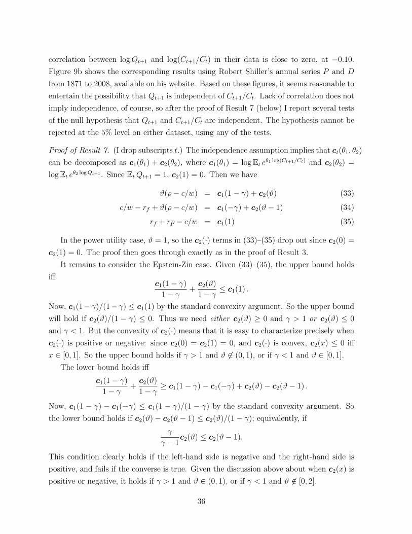
correlation between logQt+1 and log(Ct+1/Ct) in their data is close to zero, at −0.10.

Figure 9b shows the corresponding results using Robert Shiller’s annual series P and D

from 1871 to 2008, available on his website. Based on these figures, it seems reasonable to

entertain the possibility that Qt+1 is independent of Ct+1/Ct. Lack of correlation does not

imply independence, of course, so after the proof of Result 7 (below) I report several tests

of the null hypothesis that Qt+1 and Ct+1/Ct are independent. The hypothesis cannot be

rejected at the 5% level on either dataset, using any of the tests.

Proof of Result 7. (I drop subscripts t.) The independence assumption implies that ct(θ1, θ2)

can be decomposed as c1(θ1) + c2(θ2), where c1(θ1) = logEt eθ1 log(Ct+1/Ct) and c2(θ2) =

logEt eθ2 logQt+1 . Since EtQt+1 = 1, c2(1) = 0. Then we have

ϑ(ρ− c/w) = c1(1− γ) + c2(ϑ) (33)

c/w − rf + ϑ(ρ− c/w) = c1(−γ) + c2(ϑ− 1) (34)

rf + rp− c/w = c1(1) (35)

In the power utility case, ϑ = 1, so the c2(·) terms in (33)–(35) drop out since c2(0) =

c2(1) = 0. The proof then goes through exactly as in the proof of Result 3.

It remains to consider the Epstein-Zin case. Given (33)–(35), the upper bound holds

iffc1(1− γ)

1− γ+

c2(ϑ)

1− γ≤ c1(1) .

Now, c1(1−γ)/(1−γ) ≤ c1(1) by the standard convexity argument. So the upper bound

will hold if c2(ϑ)/(1 − γ) ≤ 0. Thus we need either c2(ϑ) ≥ 0 and γ > 1 or c2(ϑ) ≤ 0

and γ < 1. But the convexity of c2(·) means that it is easy to characterize precisely when

c2(·) is positive or negative: since c2(0) = c2(1) = 0, and c2(·) is convex, c2(x) ≤ 0 iff

x ∈ [0, 1]. So the upper bound holds if γ > 1 and ϑ 6∈ (0, 1), or if γ < 1 and ϑ ∈ [0, 1].

The lower bound holds iff

c1(1− γ)

1− γ+

c2(ϑ)

1− γ≥ c1(1− γ)− c1(−γ) + c2(ϑ)− c2(ϑ− 1) .

Now, c1(1 − γ) − c1(−γ) ≤ c1(1 − γ)/(1 − γ) by the standard convexity argument. So

the lower bound holds if c2(ϑ)− c2(ϑ− 1) ≤ c2(ϑ)/(1− γ); equivalently, if

γ

γ − 1c2(ϑ) ≤ c2(ϑ− 1).

This condition clearly holds if the left-hand side is negative and the right-hand side is

positive, and fails if the converse is true. Given the discussion above about when c2(x) is

positive or negative, it holds if γ > 1 and ϑ ∈ (0, 1), or if γ < 1 and ϑ 6∈ [0, 2].

36

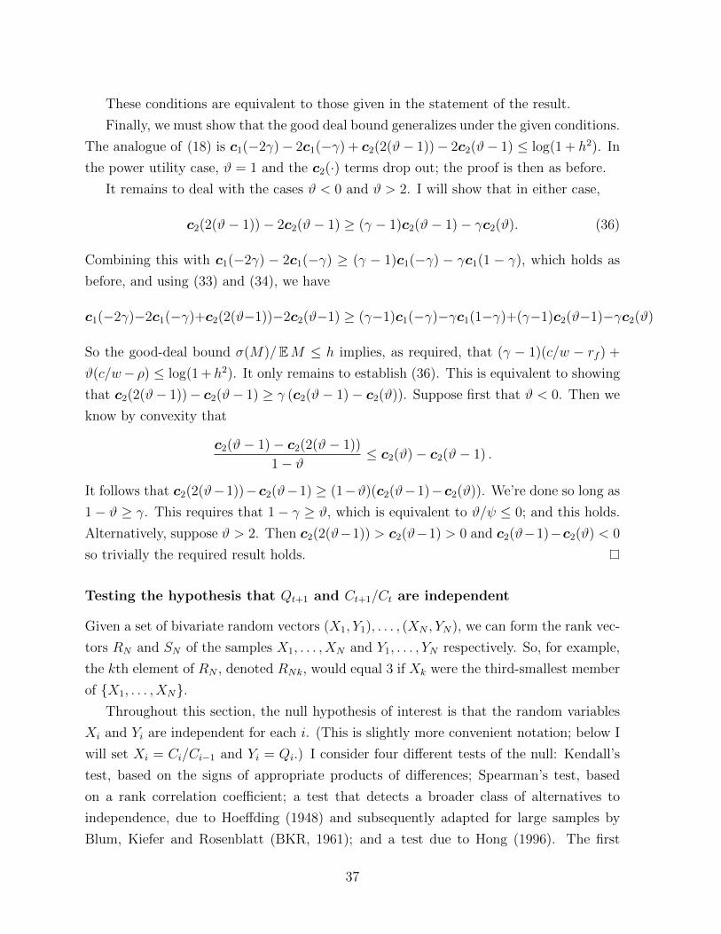
These conditions are equivalent to those given in the statement of the result.

Finally, we must show that the good deal bound generalizes under the given conditions.

The analogue of (18) is c1(−2γ)− 2c1(−γ) + c2(2(ϑ− 1))− 2c2(ϑ− 1) ≤ log(1 + h2). In

the power utility case, ϑ = 1 and the c2(·) terms drop out; the proof is then as before.

It remains to deal with the cases ϑ < 0 and ϑ > 2. I will show that in either case,

c2(2(ϑ− 1))− 2c2(ϑ− 1) ≥ (γ − 1)c2(ϑ− 1)− γc2(ϑ). (36)

Combining this with c1(−2γ) − 2c1(−γ) ≥ (γ − 1)c1(−γ) − γc1(1 − γ), which holds as

before, and using (33) and (34), we have

c1(−2γ)−2c1(−γ)+c2(2(ϑ−1))−2c2(ϑ−1) ≥ (γ−1)c1(−γ)−γc1(1−γ)+(γ−1)c2(ϑ−1)−γc2(ϑ)

So the good-deal bound σ(M)/EM ≤ h implies, as required, that (γ − 1)(c/w − rf ) +

ϑ(c/w− ρ) ≤ log(1 +h2). It only remains to establish (36). This is equivalent to showing

that c2(2(ϑ− 1))− c2(ϑ− 1) ≥ γ (c2(ϑ− 1)− c2(ϑ)). Suppose first that ϑ < 0. Then we

know by convexity that

c2(ϑ− 1)− c2(2(ϑ− 1))

1− ϑ≤ c2(ϑ)− c2(ϑ− 1) .

It follows that c2(2(ϑ−1))−c2(ϑ−1) ≥ (1−ϑ)(c2(ϑ−1)−c2(ϑ)). We’re done so long as

1− ϑ ≥ γ. This requires that 1− γ ≥ ϑ, which is equivalent to ϑ/ψ ≤ 0; and this holds.

Alternatively, suppose ϑ > 2. Then c2(2(ϑ−1)) > c2(ϑ−1) > 0 and c2(ϑ−1)−c2(ϑ) < 0

so trivially the required result holds.

Testing the hypothesis that Qt+1 and Ct+1/Ct are independent

Given a set of bivariate random vectors (X1, Y1), . . . , (XN , YN), we can form the rank vec-

tors RN and SN of the samples X1, . . . , XN and Y1, . . . , YN respectively. So, for example,

the kth element of RN , denoted RNk, would equal 3 if Xk were the third-smallest member

of {X1, . . . , XN}.Throughout this section, the null hypothesis of interest is that the random variables

Xi and Yi are independent for each i. (This is slightly more convenient notation; below I

will set Xi = Ci/Ci−1 and Yi = Qi.) I consider four different tests of the null: Kendall’s

test, based on the signs of appropriate products of differences; Spearman’s test, based

on a rank correlation coefficient; a test that detects a broader class of alternatives to

independence, due to Hoeffding (1948) and subsequently adapted for large samples by

Blum, Kiefer and Rosenblatt (BKR, 1961); and a test due to Hong (1996). The first

37

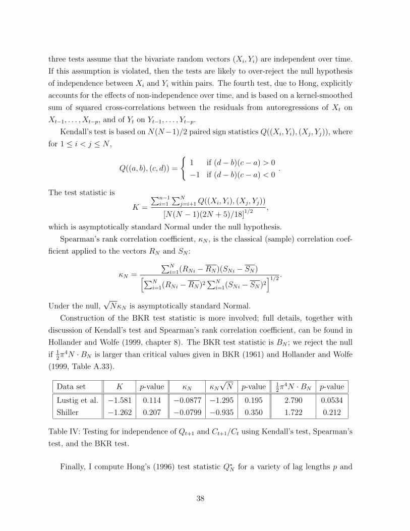
three tests assume that the bivariate random vectors (Xi, Yi) are independent over time.

If this assumption is violated, then the tests are likely to over-reject the null hypothesis

of independence between Xi and Yi within pairs. The fourth test, due to Hong, explicitly

accounts for the effects of non-independence over time, and is based on a kernel-smoothed

sum of squared cross-correlations between the residuals from autoregressions of Xt on

Xt−1, . . . , Xt−p, and of Yt on Yt−1, . . . , Yt−p.

Kendall’s test is based on N(N−1)/2 paired sign statistics Q((Xi, Yi), (Xj, Yj)), where

for 1 ≤ i < j ≤ N ,

Q((a, b), (c, d)) =

{1 if (d− b)(c− a) > 0

−1 if (d− b)(c− a) < 0.

The test statistic is

K =

∑n−1i=1

∑Nj=i+1Q((Xi, Yi), (Xj, Yj))

[N(N − 1)(2N + 5)/18]1/2,

which is asymptotically standard Normal under the null hypothesis.

Spearman’s rank correlation coefficient, κN , is the classical (sample) correlation coef-

ficient applied to the vectors RN and SN :

κN =

∑Ni=1(RNi −RN)(SNi − SN)[∑N

i=1(RNi −RN)2∑N

i=1(SNi − SN)2]1/2 .

Under the null,√NκN is asymptotically standard Normal.

Construction of the BKR test statistic is more involved; full details, together with

discussion of Kendall’s test and Spearman’s rank correlation coefficient, can be found in

Hollander and Wolfe (1999, chapter 8). The BKR test statistic is BN ; we reject the null

if 12π4N ·BN is larger than critical values given in BKR (1961) and Hollander and Wolfe

(1999, Table A.33).

Data set K p-value κN κN√N p-value 1

2π4N ·BN p-value

Lustig et al. −1.581 0.114 −0.0877 −1.295 0.195 2.790 0.0534

Shiller −1.262 0.207 −0.0799 −0.935 0.350 1.722 0.212

Table IV: Testing for independence of Qt+1 and Ct+1/Ct using Kendall’s test, Spearman’s

test, and the BKR test.

Finally, I compute Hong’s (1996) test statistic Q∗N for a variety of lag lengths p and

38

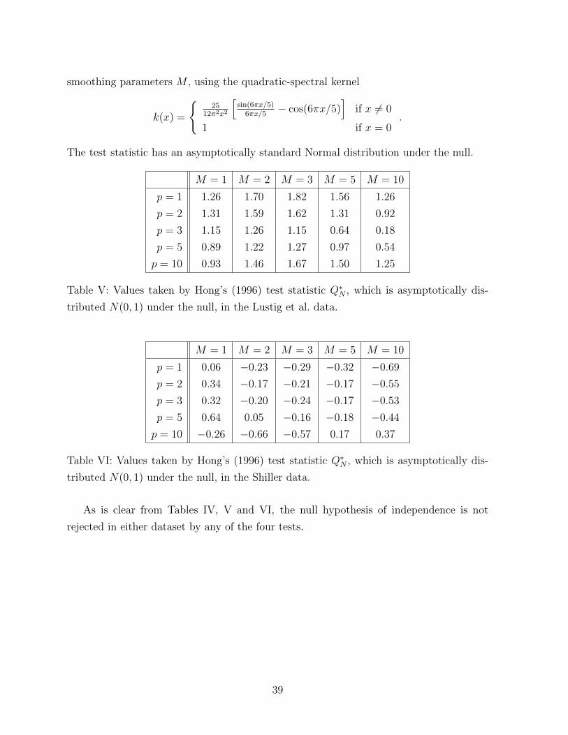
smoothing parameters M , using the quadratic-spectral kernel

k(x) =

{25

12π2x2

[sin(6πx/5)

6πx/5− cos(6πx/5)

]if x 6= 0

1 if x = 0.

The test statistic has an asymptotically standard Normal distribution under the null.

M = 1 M = 2 M = 3 M = 5 M = 10

p = 1 1.26 1.70 1.82 1.56 1.26

p = 2 1.31 1.59 1.62 1.31 0.92

p = 3 1.15 1.26 1.15 0.64 0.18

p = 5 0.89 1.22 1.27 0.97 0.54

p = 10 0.93 1.46 1.67 1.50 1.25

Table V: Values taken by Hong’s (1996) test statistic Q∗N , which is asymptotically dis-

tributed N(0, 1) under the null, in the Lustig et al. data.

M = 1 M = 2 M = 3 M = 5 M = 10

p = 1 0.06 −0.23 −0.29 −0.32 −0.69

p = 2 0.34 −0.17 −0.21 −0.17 −0.55

p = 3 0.32 −0.20 −0.24 −0.17 −0.53

p = 5 0.64 0.05 −0.16 −0.18 −0.44

p = 10 −0.26 −0.66 −0.57 0.17 0.37

Table VI: Values taken by Hong’s (1996) test statistic Q∗N , which is asymptotically dis-

tributed N(0, 1) under the null, in the Shiller data.

As is clear from Tables IV, V and VI, the null hypothesis of independence is not

rejected in either dataset by any of the four tests.

39