CONSEQUENCE MODELLING OF HAZARDOUS STORAGES

3.1 INTRODUCTION

CONSEQUENCE MODELLING OF HAZARDOUS STORAGES

Consequence modelling refers to the calculation or estimation of

numerical values (or graphical representation) that describes the credible

physical outcomes of loss of containment scenarios involving f1ammablc,

explosive and toxic materials with respect to their impact on people, assets or

safety functions [1]. The need t()[ risk assessment and consequence modell ing

of process plant and hazardous storage facilities has become exceedingly

critical due to the trend towards larger and more complex units that process

toxic, flammable and otherwise hazardous chemicals under extreme

temperature and pressure conditions. Moreover, the proximity of many such

units to densely populated areas may magnify the potential damage

One of the most powerful and widely used concepts in risk assessment

methodologies is quantified risk analysis (QRA) [2]. It involves the following

steps

a. Development of credible accident scenarios.

b. Damage calculations through mathematical modelling. The impact

of the scenarios is studied using available models such as VCE

modelling, BLEVE modelling etc.

Chapter 3

c. Risk estimation. Based on the damage potential estimated in the

previous steps and the probability of occurrcnce of these credible

accident scenarios, risk factors are estimated.

Quantitied risk analysis (QRA) is the most effective way to represent the

socictal risks associated with MAH installations [3]. Increasing public

awareness of technological risk has placcd a greater responsibility on the

process industries and district authorities to review and revise their current

satety practices to make the process technologies both intrinsically and

extrinsically safer. Consequence analysis is a tool which quantifies the

consequences from the hazardous storages in the MAH industries.

Fire is a process of burning that produces heat, light and often smokes

and flame [4]. Fire or combustion is detined by F.P Lees [5J as a chemical

reaction in which a substance combines with oxygen and heat is released.

Combustion is defined by NFP A [4] as an exothermic, self-sustaining reaction

involving solid, liquid, and for gas-phase fuel.

There are various classes of fire like Class A, Class B, Class C, and

Class 0 [6, 7] based on the burning material involved. The tire associated with

chemicals can take several different forms like flash tire, jet tire, and pool fire

(8,9]. A flash fire is the non explosive combustion of a vapor cloud resulting

from the release of a flammable material in to the open air [8]. The speed of

burning is a function of the concentration of the flammable component in the

cloud and also the wind speed [10, 11]. Within a tew second of ignition the

flame spreads both upwind and downwind of the ignition source. Initially the

flame is contained within the cloud due to prcmixed burning of the regions

within the flammable limits. Subsequently the flame extends in the form of a

fire plume above the cloud. The downwind edge of the tlame starts to move

towards the spill point after consuming the flammable vapor downwind of the

Consequence modellillg o(hazardolls storages

ignition source. Typical flame propagation speeds are of the order of 4 m/s [9,

10]. The flame velocity and dispersion increases with the wind speed. The

duration of this fire is very short and the damage is caused by thermal radiation

and oxygen depletion.

A jet fire occurs when a flammable liquid or gas is ignited after its

release from a pressurized, punctured vessel or pipe [8]. The pressure of release

generates a long flame, which is stable under most conditions. A flash flame

may take the form of jet flame on reaching the spill point. The release ratc and

the capacity of the source detennine the duration of the jet tire. Flame length

increases directly with f10w rate. Typically a pressurized release of 8 kg/s

would have a length of 35 m [9). The crosswinds also affect the flame length.

An increase in the crosswind velocity increases the name length. A pool fire

occurs on ignition of an accumulation of liquid as a pool 011 the ground or on

water or other liquid [9]. A steadily burning tire is rapidly achieved as the vapor

to sustain the fire is provided by evaporation of liquid by heat from the flames.

The maximum burning rate is a function of the net heat of combustion and heat

required for its vaporization. Generally heat radiation dominates the burning

rate for flame greater than I m diameter. Fire modelling of flammable substance

like naphtha, benzene, cyclohexane, cyclohexanone and ammonia are carried

out and results are discussed in this chapter.

Several definitions are available for the word "'explosion".

AIChE/CCPS [12] defines an explosion as "a release of energy that causes a

blast". A blast is subsequently defined by CCPS as ··a transient change in the

gas density, pressure and velocity of the air surrounding an explosion poinf'.

Crowl and Louvar [13] define an explosion as "a rapid expansion of gases

resulting in a rapidly moving pressure or shock wave". NFPA 69[14] defines an

explosion as "the bursting or rupture of an enclosure or a container due to the

Chapter 3

development of internal pressure". Explosion generally occurs in situations

where the fuel and oxidant have been allowed to mix intimately before ignition

[4].

The injuries and damage are in the ti.rst place caused by the shock wave

of the explosion itself [91. People are blown over or knocked down and buried

under collapsed buildings or injured by flying glass. Although the effects of

overpressurc can directly result in deaths, this would be likely to involve only

those working in the direct vicinity of the explosion [9]. The history of

industrial explosions shows that the indirect effects of collapsing buildings,

flying glass and debris cause far more loss of life and severe injuries. The

effects of the shock wave vary depending on the characteristics of the material,

the quantity involved and the degree of confinement of the vapor cloud. The

peak pressure in an explosion therefore varies between a slight over-pressure

and a few hundred kilo Pascal (kPa). Direct injury to people occurs at pressures

of 5-10 kPa with loss of life generally occurring at a greater over pressure,

whereas dwellings are demolished and windows and doors broken at pressure

of as low as 3-10 kPa. The pressure of the shock wave decreases rapidly with

increase in the distance from the source of the explosion [8, 9]. As an example,

the explosion ofa tank containing 50 tonnes of propane results in pressure of 14

kPa at 250 meters and pressure of 5 kPa at 500 meters from the tarue

The effects of toxic chemicals when considering major hazards, on the

other hand, are quite different and are concerned with the acute exposure during

and soon after a major accident rather than with long term chronic exposures

[15]. This chapter considers the storage and use of toxic chemicals, which

would disperse with the wind and have the potential to kill or injure people

living many hundreds of meters away ft'om the plant, and being unable to

escape or find shelter. Chemicals like chlorine, ammonia and methyl isocyanate

COl/sequence modelling Clt"hllzardolls stD/·ages

are highly toxic materials and have history of major accidents. The dispersion

modelling is an efficient tool to predict the affected area during a massive toxic

gas release and this will be useful tor the effective evacuation of people in the

affected areas.

A survey can-ied out in the MAH units 111 Udyogamandal as per

Manufacture storage and import of hazardous chemicals (MSIHC) Rules, 19~9,

India [16] and The chemical accidents ( Emergency planning, preparedness and

response) Rules, 1996, India [17] revealed that the major hazardous chemicals

stored by the various industrial units are anunonia, chlorine, benzene, naphtha,

cyclohexane, cyclohexanone and LPG. The damage potential of these chemicals

is assessed using consequence modelling. Modelling of pool fires t()f naphtha,

cyclohexane, cyelohexanom:, benzene and ammonia are carried out using TNO

model demonstrated in World Bank tcchnical paper No.55 [18) and G. Madhu

[19). Vapor cloud explosion (VCE) modelling of LPG, cyclohexane and

benzene are carried out usmg TNT equivalent model explained by

AIChE/CCPS [8). Boiling liquid expanding vapor explosion (BLEVE)

modelling of LPG is also considered. BLEVE is defined by CCPS [8] as a

sudden release of large mass of pressurized superheated liquid to the

atmosphere. In our study the LPG storages are pressurized storages and benzene

and eyclohexane storages are atmospheric storage. In the case of releases from

liquefied gas storages, there is a possibility of both BLEVE and VCE. The

liquefied gas that expands inside the storage vessel can lead to BLEVE whereas

the vapor that comes over to atmosphere will result in an unconflned vapor

cloud explosion. In the case of flammable liquids like benzene, and

eyelohexane, the leakage or spillage hom a storage tank may first t<.mn a pool

outside and the vapors generated tl"om the pool may cause a VCE in the

presence of an ignition source. Another possibility is the escape of benzene or

Chapter 3

cyclohexane vapors from high temperature processes leading to an uncontined

vapor cloud explosion. Dispersion modelling of toxic chemicals like chlorine,

ammonia and benzene are analysed using ALOHA (Arial Locations of

Hazardous atmosphere) [20] air quality model. For these analyses heat of

combustion, heat of vaporization, specific heat at constant pressure and boiling

point of the above hazardous chemicals are necessary. These values are

obtained fi·om Perry's Chemical engineers Handbook [21], Petroleum relining

engineering [22J and CAMEO (Computer aided management in emergency

operations) [23].

3.2 MODELLING OF POOL FIRES

Pool tire is a conunon type of fire, which can occur in the t<mn of a tank

fire or fi:ol11 a pool of fuel spread over a ground or water. A pool tire occurs

when a flammable liquid spills into the ground and is ignited. A fire in a liquid

storage tank and a trench tire are forms of pool fire. It has been observed that

the characteristics of pool fire depend on the pool diameter [8]. Different

authors have suggested a number of pool fire models. An empirical model

commonly employed in the estimation ofradiative flux from a pool fire is TNO

model [18, 19]. This model uses classical empirical equations to determine

burning rate, heat radiation and incident heat. For liquids with boiling point

above ambient temperature, the rate of burning of the liquid surface per unit

area is given by

dill

ilt _---;--0_, 0_0_1-,-1 '-'-.' ______________ (3. 1)

C/I (T" - 1',,)+ HI""

Consequence modelling of hazardous storages

where He - heat of combustion (J/kg), Cl' - Specific heat at constant pressure

(J/kg K), ~ - boiling point in (K), 7;, - ambient temperature (K), HmI' - heat of

vaporization (J/kg).

For liquids with a boiling point below ambient temp, the expression is

dm = O.OOIH, -----(3.2) dt H'(lfI

The total heat t1ux from a pool of radius "r" (meters) is given by

( 0 )[ dm] nr' + 2TIrll -dl-- "He

Q = -----(33)

[ ]

111>1 •

72 dm +1 dt

where Q - total heat t1ux (W/I11~), H-t1ame height (m), '7- efficiency factor.

The efficiency factor of total combustion power is often quoted in the range of

0.15-0.35 [24, 25].

Flame height is given by G. Heskestad [26] as

, , H = 0.235Q~) -1.02D------(3.4)

Where D is the diameter of the storage tank (m)

Q is the total heat released by fire (kW/m~)

The intensity of heat radiation at a distance R from the pool centre is

given by

TQ 1= ------(3.5)

4rIR2

where r - transmissivity of air path, Q - total heat flux (W/m2).

Chapter 3

Burning rate and flame height are empirical but are well established

methods for the detennination of intensity of heat rad iation [8J.

The effects of intensity of heat radiat io n on huma n being and materials

arc g iven in Table 3. 1.

Table 3.1 Various effects of intensity of heat radi<.ltion

1.6

2.2

4.2

8.3

10.8

15.0

25.0

4.0

12.0

19.0

37.5

100.0

Insufficient to cause no discomt'llrt for long exposure.

Threshold pain. No reddening or blister.

Firs! degree burn

Second degree burn

Third degree burn

Piloted ignition of wood

Spontaneous ignition of wood

Glass cracks

Plastic melts

Cable insula~ion degrades

Damage to process equipment

Steel structure fail .. ,.

CQlIseqllem:e mode//illg o/IWUlrdolls s/omges

3.3 MODELLING OF EXPLOSION

There are severa l types of explosion including detlagration, detonat ion,

dust explosion, vapor cloud explosion and boiling liquid expanding vapour

explosion (BLEVE).

0. 14

0.28

0.69

1.03

6.9

9.0

13 .8

48.2

62.0

68 .7

2068

Table 3.2 Various effects of pressure wave

Annoying noise (137 dB)

Loud noise (143 dB)

strain

damage to window frames.

damage to house structure

Pa.1ia l demo lition of houses

Steel frame slight ly distorted

Partia l co llapse

50% of house

10

wagon

etc.

Limit

Safe distance

process qlluntiWtil'l!

Chapter 3

3.3.1 Modelling ofvapor cloud explosion (VCE)

When a large amount of flammable vaporizing liquid or gas is rapidly

released, a vapor cloud ttlrms and disperses with the surrounding air. The

release can occur fi'om a storage tank, process, transport vessel. or pipelines. If

this cloud is ignited bcft)re the cloud is dilut<.:d below its lo\ver flammability

limit (LFL), a vapour cloud explosion (VCE) will occur. Centre t(Jr Chemical

Process Safety (CCPS) of American Institute of Chemical Engineers [9]

provides an excellent summary of vapour cloud behaviour. They describe four

features, which must be present for a VCE to occur. First the release material

must be flammable. Second, a cloud of sufficient size must form prior to

ignition. Third, a sufficient amount of the cloud must be within the flammable

range. Fourth, suftlcient confinement or turbulent mixing of a p011ion of the

vapor cloud must be present [8].

Following models are used for VCE modelling

I. TNT equivalent model

2. TNO multi energy model

3. Moditied Baker model

All of these models are quasi-theoretical and are based on the limited

tield data and accident investigation. TNT equivalency model is easy to use and

has been applied for many QRA studies [8]. It is described in Baker [27],

Decker [28], Lees [5] and Merex [29]. TNT model is well established for high

explosives but when applied to flammable vapour clouds it requires the

explosion yield '7 , determined from the past incidents. Following methods arc

used for estimating the explosion efficiency.

COl/sequence modelling ()( hazardous sloragcs

l.Braise and Simpson [30] uses 2% to 5% of the heat of combustion of the

total quantity of fuel spilled.

2. Health and Safety Executive [31, 32] uses 3% of thc heat of combustion

ofthc quantity offucl present in thc cloud.

3.Industrial Risk Insures [33] uses 2% of the heat of combustion of the

quantity ofthe fuel spilled.

4. Factory Mutua1 Research Corporation [34] uses 5%, 10% and 15% of the

heat of combustion of the quantity offuel present in the cloud, dependant

on the reactivity ofthe materiaL

3.3.2 TNT Equivalent model for VCE

The TNT equivalent model [5, 8, 29] is based on the assumption of

equivalence between the flammable material and TNT tactored by an explosion

efficiency term. The TNT equivalent W is given by

llMHc W = -----(3.6)

ETNT

where W - equivalent mass of TNT (kg), '7 - empirical explosion efficiency,

M- mass of hydrocarbon (kg), He - heat of combustion of flammab1e substance

(J/kg), En! - heat of combustion of TNT (J/kg).

3.3.2.1 PresslI re (~l blast wave

The explosion of a TNT charge is shown in Fig. 3.1 for a hemispherical

TNT surface charge at sea level. The pressure wave effects arc correlated as a

Chapler 3

function of scaled range. The scaled range is defined as distance X by the cube

root of TNT mass.

x Z = - , . ---- -(3.7)

WYj

where Z · scaled distance in the graph. X· Radia l distance from the surface of

the fire ba ll (m), W - TNT equi va lent (kg).

Using X and W, we can find out Z. From the graph we can find out over

pressure corresponding to Z. Table 3.2 provides various effects of blast over

pressure to human being and materials.

10'

• 10'

Q,

l!~~ 10' _ .. ~

!:. - 10' ;-..., o --: -Ill] 100

lOt

10" 10' 10' 100 10' 10'

Scaled Distance, Z (mlkg13)

Fig. 3.1 Scaled distance vs. overpressure for VCE

(Source: AIChElCCPS. Guideline for chemical process quantitative risk analysis)

Consequellce modelling 0/ hazardous slorages

3.3.3 Modelling of boiling liquid expanding vapor explosion (BLEVE)

Among the diverse major accidents which can occur in process

industries, in energy installations and in the transportation of dangerous

materials, Boiling liquid expanding vapor explosions or BLEVEs arc important

especially due to their severity and the tact that they involve simultaneously

diverse effects which can cover large areas, overpressure , thermal radiation and

missile efiect [35]. Boiling liquid expanding vapor explosion (BLEVE) is a

type of physical explosion that can affect almost any liquid contained in a

closed vessel at a temperature significantly higher than its boiling point at

atmospheric pressure [8,36]. The physical force that causes the BLEVE is on

account of the large liquid to vapor expansion of the liquid in the container.

LPG will expand to 250 times its volume when changing from liquid to vapor.

It is this expansion process that provides the energy for propulsion of the

container and the rapid mixing ofvapor from the container with air, resulting in

the fireball characteristic when flammable liquids are involved. Boiling Liquid

expanding vapour explosions were defined by Walls [37], who first proposed

the acronym BLEVE as Ha failure of a major container into two or more pieces

occurring at a moment where the container is at a temperature above boiling

point at normal atmospheric pressure.

In most BLEVE cases caused by exposure to fire, the container failure

originates in the container metal significantly where it is not in contact with

liquid. The liquid conducts the heat away from the metal and acts as a heat

absorber. Therefore the metal around the vapor space can be heated to the point

of failure. The major hazards of BLEVE are thermal radiation, velocity of

fragments and over pressure from shock wave.

Chapfer 3

3.3.3.1 Radiation received by a target

The radiation rc(;cived hy a receptor (for the duration of BLEVE

incident) is given by (,CPS of AIChE [8] as.

E = r EF - - - - - (3 8) • ...1 r et ~ I .

where 1:', - cmissivc radiativc nux received hy a I'cccptor (W/m\ f,,-

transmissivity (dimension less), E -surface emitted radiative tlux (W/m\ 1'~1 -

view factor (dimensionless).

Roberts [38], Hymes [391 and CC PS [8] provide a means to estimate

surface heat flux based on the radiative fraction of the total heat of combustion.

E:::::; RM~(' ------(3.9) ITDmax - t blel'e

where E - radiative emissive flux (W Im\ R - radiation fraction of heat of

combustion (dimensionless), M - initial mass of fuel in the fire ball (kg), He-

heat of combustion per unit mass (J/kg), Dmax - maximum diameter of tire balls

(m), tbleve - duration oft1reballs

Hymes [39] suggest the following values for R, 0.3 for fireball from

vessel bursting below the relief set pressure and 0.4 for fireballs from vessels

bursting at or above the relief set pressure.

COllsequence /JlodellinK of'lw::ardolls .,"(orages

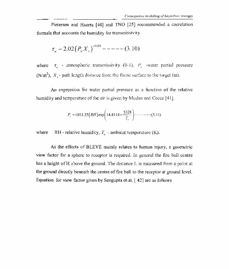
Pietersen and Huerta [40] and TNO [25] recommended a correlation

formula that accounts the humidity for transmissivity.

= 2.02(P X )-0.09 -----(3.10) Ta It· s

where la - atmospheric transmissivity (0-1). f~! -water partial pressure

(N/m\ Xs - path length distance !l'om the flame surface to the target (m).

An expression for water pat1ial pressure as a function of the relative

humidity and temperature of the air is given hy M udan and Corcc [411.

( 532S J P.. = !013.25(RH)exp 14.4114-~ ------(3.11)

where RH - relative humidity, 7;, - ambient temperature (K).

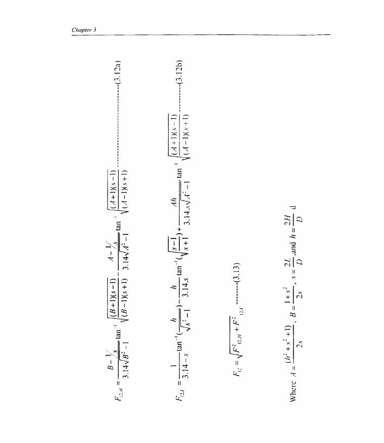
As the effects of BLEVE mainly relates to human injury, a geometric

view factor for a sphere to receptor is required. In general the fire ball centre

has a height of H above the ground. The distance L is measured B:om a point at

the ground directly beneath the centre of fire ball to the receptor at ground level.

Equation for view factor given by Sengupta et.a!' [ 42] arc as follows

fJ { ~ <..

..

8-

t/

F;".I

I =

,/

s 3

.14

J B~

-I t

an'!

(B

+ l)

(s -

I) _

A

-,~:

ta

n!

I ( A +

1 )( s

-I)

___

____

____

____

____

____

____

___ (

3. I

la)

(B -

l)( s

+ I)

3.

14

J A ~ -

I V

( A-I

)(s

+ I )

~ 1

·-1

" h

) h-!(J§~,-I)

Ah

! J

(A+

1)(,

<; ..

.. 1)

,

I' ~

, =

tan

( -

tan

-+

ta

n --

----

----

(3.1

2b)

1-.1

3.1

4-s

.J

s2-1

3.1

4.s

s+

l 3.

14 .. \

''''

'A~-

1 (A

-I)(

s+

l)

p,

=

r p2

+ F

= --

----

--(3

.13)

L

V

1':

'.11

12.1

'

WI

I (/1

2 +

s:

+ 1)

B

1+

",2

2L

d J

2H

I lc

re /

~

" =

--

s ~ -

,an

1 = -

( ."

' .,.'

D'

D'

_.\

-,

~

Conseqllence II/odelling (d'hazardous storages

Pitblado [ 43 J developed correlation for BLEVE fIre ball diameter as a

function of mass released and Tasneem Abbasi ct.al. [44J compared the various

correlations for BLEVE fIre ball diameter calculation. The TNO formula

proposed by Peterson and Huerta [401 give good overall tit to observed data.

All models use power law correlations to relate BLEVE diametcr and duration

to the mass.

Empirical equations f(lT maXllllum diameter of tire ball, duration of

BLEVE and distance between the fireball centre and the ground given by

AIChE/CCPS {12l are as f()llows

, [I

D ;::;:5.8MI' ------(3 14) 1l1,aX •

1/ t -'>6M/6------(31S) hle\"e - -. • ...

lIb/e,.!' =O.75Dm .. , -----(3.16)

where, M is the initial mass of the flammable material in kg.

3.3.3.2 Fragments and their effects

The prediction of fragments effects is important, as many death and

domino damages effects are attributable to them. Specific work on BLEVE

fragmentation was carried out by Association of American Railroads and by

Holden and Reeves [45]. Fragments are usually not evenly distributed. The

vessel's axial direction receives more fragments than the side directions. The

total number of fragments is approximately a fraction of vessel size. Ho Iden and

Reeves [45] suggest a correlation based on seven incidents (Eq. 3.17) is listed

by Tasneem Abbasi et.al. [44].

N = -3.77 + 0.0096 V------------- (3.17)

Chapter 3

where N is the number of fragments, V is the vessel capacity in m3• But this

equation is valid only fi)r the range of 700-2500 m3. The correlation curves

given by Holden and Reeves can be extrapolated for use in other ranges.

BLEvEs typically produce fewer fi'ugments than high-pressure

detonation. (Between 2 and 10 arc typical) [8]. From the inner and outer

diameter of the vessel, thickness of the vessel is estimated and the total mass of

the vessel is also estimated using the density of the material. Appropriate

assumptions can be made for the BLEvE scenarios LX, 46J i()r number of

fragments. Total mass divided by the assumed number of fragments gives the

average mass of one fragment. The average mass of the fi'agment is estimated

by assuming that each shell fragment is crumbled up into spheres. BLEVEs

usually do not develop high pressure that leads to greater fragmentation.

Instead, metal softening from the heat exposure and thinning of the vessel will

yield fewer fragments. Normally LPG storage tanks are designed for 250 psig

working pressure. A normal burst pressure of four times the working pressure is

expected for ASME coded vessels. Stawczyk [46J in a study of LPG cylinder of

5 kg and 11 kg capacities found that each BLEvEs gives three to five main

projectiles and several smaller fragments.

BLEVEs usually occur because of flame impingement on the un-wetted

portion (vapor space) of the tanle This area becomes sufficiently weakened and

the tank fails at approximately 300 - 400 psig.

3.3.3.3 Velocity offragments

Baker et.al. [27] and Brown [47] provide formulas f()r prediction of

projectile effects. They consider fracture of cylindrical and spherical vessels

CO/lsequence modelling (~lhazardolls storages

into 2, 10 and 100 fragments. Typically for these types of events, only 2 or 3

fragments occur.

The first part of the calculation involves the estimation of an initial

velocity. Once fragments are accelerated they will fly through the air until they

impact another object or target on the ground. The second part of the

calculation involves the estimation of the distance a projectile could travel.

For pressurized vessels, initial velocity of a tl-agment is given hy

Moorce [48]

)PD' II = 3.356 W ------(3.18)

where u - initial velocity (m/sce), P - rupture pressure of the vessel (NI m\ 0 -

fragment diameter (meters), W- weight of the fragment (Kg).

3.3.3.4 Distance travelled by thefragmellt.

From simple physics, it is well known that an object will fly the greatest

distance at a trajectory angle of 45°

The maximum distance is given by Baum [49]

u -----(3.19)

g

3.3.3.5 Pressure of blast wave due to BLEVE

Procedure for detennining the ovcrpressure at a distance from a storage

vessel is given by Baker et. aI., [27] and Prugh [50].

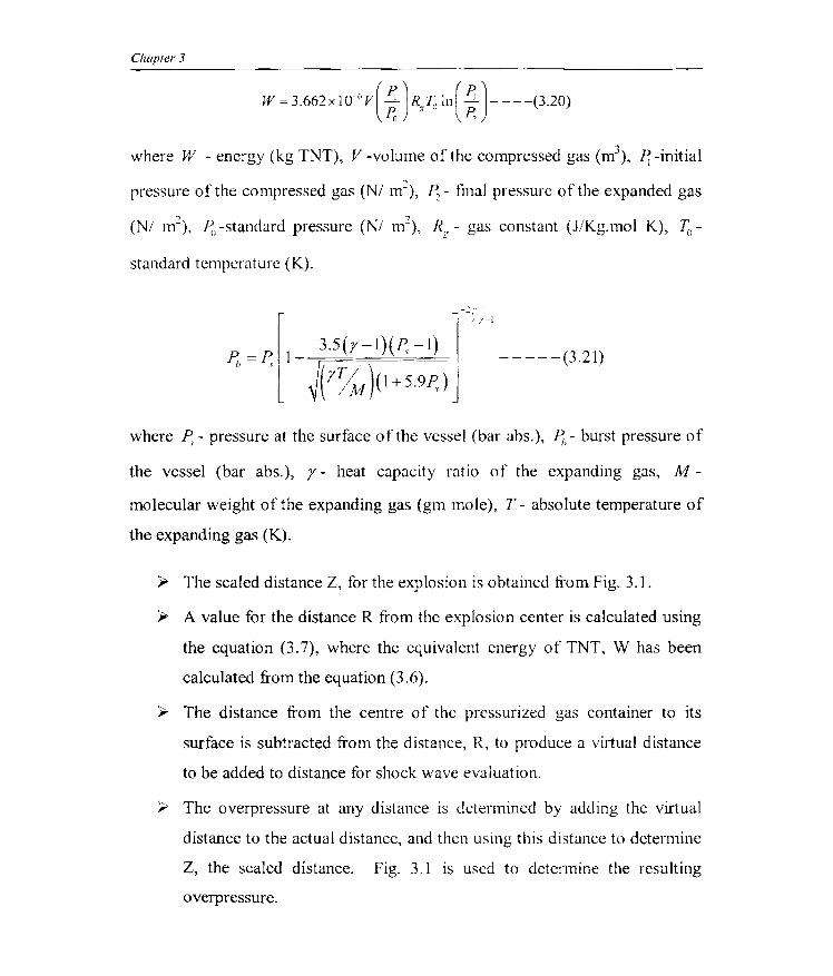
Chapter 3

HI = 3.662x 1O-6V(~ )RJo In( ~)- ---(3.20) ~I ~

where W - energy (kg TNT), V -volume oftht; compressed gas (m\ ~ -initial

pressure of the compressed gas (NI m~), ~ - final pressure of the expanded gas

(NI m~), ~I -standard pressure (NI m\ RI' - gas constant (J/Kg. 1110 I K), ~)

standard temperature (K).

, ..

~,= ~[l- 3'5(r-l)(p~l'>' -----(3.21)

(rJ~ )(1 + 5.9p,)

where p. - pressure at the surface of the vcssel (bar abs.), 11, - burst pressure of

the vessel (bar abs.), r - heat capacity ratio of the expanding gas, M

molecular weight of the expanding gas (gm mole), T - absolute temperature of

the expanding gas (K).

>- The scaled distance Z, for the explosion is obtained tt'om Fig. 3.1.

';r A value for the distance R from the t;xplosion center is calculated using

the equation (3.7), where the equivalent energy of TNT, W has been

calculated from the equation (3.6).

" The distance from the centrt; of the pressurized gas container to its

surface is subtracted from the distance, R, to produce a virtual distance

to be added to distance for shock wave evaluation.

';Y The overpressure at any distance is determined by adding the virtual

distance to the actual distance, and then using this distance to determine

Z, the scaled distance. Fig. 3.1 is used to determine the resulting

overpressure.

Conseqllence modelling o/Iwzardolls slorages

3.4 DISPERSION MODELLING

Dispersion [51] is a term used by modellers to include advcction

(moving) and diffusion (spreading). A dispersing vapor cloud will generally

move in a downwind direction and spread (ditluse) in a crosswind and vertical

direction (crosswind is the direction perpendicular to the wind). A cloud of gas

that is denser or heavier than air (called a heavy gas) can also spread upwind to

a small extent.

Dispersion calculations provide an estimate of the area affected and the

average vapour concentrations expected. The simplest calculations require an

estimate of the rate of the gas (or the total quantity released), the atmospheric

conditions (wind speed, time of day, cloud cover), surface roughness,

temperature, pressure and the release diameter. More complicated models may

require additional detail on the geometry, discharge mechanism, and other

information on the release. Three kinds of vapor cloud behaviour such as

neutrally buoyant gas, positively buoyant gas and dense buoyant gas are used in

different models. Three different release-time modes such as instantaneous

(putt), continuous release (plumes) and time varying continuous are also used

in different models. The well known Gaussian models describe the behaviour of

naturally buoyant gas released in the wind direction. Neutrally or positively

buoyant plume and puff have been studied for many years using Gaussian

models [8]. Dense gas plume and puffs have received more recent attention

with a number of large-scale experiments and sophisticated models heing

developed in the past 30 years [52, 53]. The concentrations pnx!ictcd hy

Gaussian models arc time averages. Thus local concentrations might be greater

than this average [8]. This result is important when estimating dispersion of

highly toxic or flammable materials where local concentration tluctuations

Chapter 3

might have significant impact on the consequences. HalU1a et.al, [54], Pasquill

& Smith [55] and Crowl & Loum [13] provide good descriptions of plume and

puff discharges.

ALOHA was designed with first responders in mind. It is intended to be

used f()r predicting the extent of the area downwind of a short-duration

chemical accident where people may be at risk of exposure to hazardous

concentrations of a toxic gas. It is not inknded for use with accidents involving

radioactive chemicals. ALOHA is also not indented to be used for stack gas or

modelling, chronic and low-level (fugitive) emissions. Since most first

responders do not havc dispersion modelling backgrounds, ALOHA has been

designed for input data that are either easily obtained or estimated at the scene

of an accident.

3.4.1 Introduction to ALOHA air modelling

ALOHA is an air dispersion model which can be used as a tool for

predicting the movement and dispersion of gases. It predicts pollutant

concentrations downwind fi·om the source of a spill, taking into consideration

the physical characteristics of the spilled material. ALOHA also accounts for

some of the physical characteristics of the release site, weather conditions, and

the circumstances of the release. Like many computer programs, it can solve

problems rapidly and provide results in a graphic easy-to-use format. This can

be helpful during an emergency response or planning for such a response.

ALOHA originated as a tool to aid in emergency response. It has

evolved over the years into a tool used t{)r a wide range of response, planning,

and academic purposes. There arc some teatures that would be useful in a

dispersion model (for example, equations accounting for site topOb'Taphy) that

CO/lSCl/IICIlCe modelling (~/hazardolls storages

have not been included in ALOHA because they would require extensive input

and computational time.

Surface topot,lfaphy can modify thc gem:ral pattem of wind speed and

direction. Onc such case is the mountain hrecze. During thc day air near the

mountain slope warms up faster than air at the same altitude but tarther tt'om

the mountain [51]. This causes a local pressure gradient towards the mountain

side and air is forced to flow up the mountain slope as mountain breeze. With

sun set the pressure gradient is reversed and the less huoyant air flows

downward into valleys.

One of the limitations of the ALOHA so fiware is that, it doesn't account

for the effects of topography. But lchikawa and Sada [56] developed a model

evaluating the topographical etlect on atmospheric dispersion using numcrical

model. In this model, the topographical eHect was evaluated in terms of the

ratios of maximum concentration and the distance of the point of maximum

concentration from the source on the topography to the respective values on a

flat plane and the relative concentration distribution along the ground surface

plume axis normalized for the maximum concentration on a f1at plane

ALOHA is intended to be used for predicting the extent of area

downwind of a chemical accident where people may be at risk of exposure to

hazardous concentrations of toxic gas. It is not intended t()r use with accidents

involving radioactive chemicals. Since most first responders do not have

dispersion modelling background, ALOHA has been designed to require input

data that are either easily obtained or estimated at the scene of an accident. The

results of toxic gas dispersion modelling are used as input data for vulncrubility

modelling.

Chapter 3

ALOHA use simplified DEGADIS [57] models and the following

assumptions are made in the original DEGADIS model

a. ALOHA - DEGADJS assumes that all heavy gas releases originates at

ground level.

h. The mathematical approximation procedure used for solving the

model's equations are taster, but less accurate than those used in

DEGADfS.

c. ALOHA-DEGADIS models sources for which release rate changes over

time as a series of short, steady releases rather than as a number of

individual point source.

ALOHA-DEGADIS was checked against DEGADIS to ensure that only

minor difference existed in results obtained from both models. Considering the

typical inaccuracies conunon in emergency response, these differences are

probably not significant.

ALOHA models the dispersion of a cloud of pollutant gas in the

atmosphere and displays a diagram that shows an overhead view of the area in

which the gas concentrations may reach hazardous levels. This diagram is

called the cloud's footprint. To obtain a footprint plot, a threshold concentration

of an airborne pollutant, usually the concentration above which the gas may

pose a hazard to people must be identified. This value is called the level of

concern (LOC). The tootprint represents the area within which the ground-level

concentration of a pollutant gas is predicted to exceed the level of concern

(LOC) at some time after a release begins.

Consequence modelling o/'hazardolls swrages

The scenario considered for analysis is tank: leak, which involves

continuous release of chlorine, ammonia and benzene. The f()llowing are the

input parameters ofALOHA.

3.4.1.1 Location information

The location selected tor the study is Eloor. The location is to be added

into the list of ALOHA.

3.4.1.2 b~tiltratioll buildillg parameters

We can specify either the type of building that is most common in the

area downwind of a chemical release or the air exchange rate that is typical of

building in that area. The choice could also represent the type of building that is

of greatest concern. ALOHA will use building type along with other

information such as wind speed and air tcmperature, to dctermine indoor

infiltration rate and to estimate indoor concentration and dose at any locations

that you specify. To estimate infiltration rate into a building, ALOHA assumes

that all doors and windows are closed.

3.4.1.3 Chemical b~tormation

The chemicals selected for the study are chlorine, ammonia and benzene. Since

these chemicals are included in the chcmical library of ALOHA, they can be

directly selected.

3.4.1.4 Atmospheric options

The information about cum:nt weather conditions 1nto ALOHA is

entered manually. ALOHA uses the in t{mnat iOIl to account for the main

processes that move and disperse a pollutant cloud within the atmosphere.

These include atmospheric heating and mechanical stirring, low-level

Chapter 3

inversions, wind speed and direction, ground roughness, and air temperature.

Wind directions and velocity are obtained from the wind roses published by the

Meteorological department of India [58].

ALOHA accounts for the ground roughness, inversion and inversion

height [59]. Ground roughness causes mechanical stirring. Atmospheric heating

is a function of inversion. Inversion height will decide whether it is low Icvel

inversion or not. ALOHA considers all these paramcters and from the available

data, it estimates the value for the above parameters.

The degree of atmospheric turbulence influences how quickly a

pollutant cloud moving downwind will mix with air around it and be diluted

below level of concern (LOC). Friction between the ground and air passing over

it is a cause of atmospheric turbulence. The rougher the ground surface, the

greater the ground that develops roughness, and greater the turbulence [8].

3.4.1.5 Tank size and orientation

When we use ALOHA's tank source option to model the release of a

liquid or gas from a storage vessel, we must indicate both the size of the tank

and its general shape.

3.4.1.6 Cre(/ible scenarios for dispersion modelling

Dispersion modelling is done by assuming the following credible

scenarios I. Leak through a hole having one inch diameter 2. Leak through a

hole having two inches diameter and 3) Catastrophic failure of the vessel.

A number of methodologies are available in the literature for the selection

of hole size

Consequence modelling of hazardolls s/orages

a. World Bank [18] suggests that characteristic hole size for pipes varies

from 20% to 100 % of the pipe diameter.

h. Some analysts use 2 inch and 4 inch holes regardlcss of the pipe size [8].

c. Some analysts use a range of hole sizes from small to large such as

0.2,1,4 and 6 inches [8].

In our study all the pipe COlllcctions to the storage vessel are of I and 2 inch

diameter and we have assumed 100% diametcr ofpipe as the hole diameter.

Dispersion modelling for catastrophic failure is done by considering an

opening large enough to release the entire mass in the storage vessel in a short

period. This situation may happen when earth quake and such natural hazards

affect the storage tank.

3.5 RESULTS AND DISCUSSION

Consequence modelling of hazardous chemicals storages like chlorine,

benzene, cyc1ohexanone, naphtha, ammonia, LPG and cyc1ohexane, are carried out.

Various input parameters provided fc)r the modelling are also given. From the

modelling of pool tires, following results are obtained. A comparison of heat

radiation for the worst case fire scenario associated with different chemical storages

from different MAH industries are presented. Hazardous distances (threat zones) for

these storages are estimated and presented in this section. Pressure effects due to

different incident scenarios like BLEVE and VCE are also estimated and presented.

Threat zones are estimated tor the pressure ettccts. Dispersion modelling is done for

different toxic scenarios and the results are compared. These results are used for the

vulnerability analysis in Chapter 4.

Chapter 3

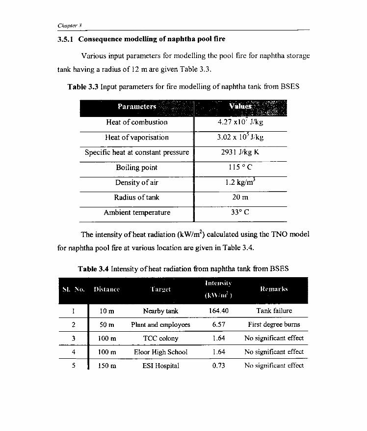
3.5.1 Consequence modelling of naphtha pool fire

Various input parameters for modelling the pool fire for naphtha storage

tank having a radius of 12 m are given Table 3.3.

Table 3.3 Input parameters for fire modelling of naphtha tank fi·om BSES

'! . . . ~ - <. ~J~~ . !~~ I

Parameters I Valu~s::: . ~>~,~,~:l;, • I _ L - ."_,-, ~ ...." .1- • .;;. .. • ... \.·., ».

Heat of combustion 4.27 xl07 J/kg

Heat of vaporisation 3.02 X 105 J/kg

Specific heat at constant pressure 2931 J/kg K

Boiling point

Density of air 1.2 kg/m3

Radius of tank 20m

Ambient temperature

The intensity of heat radiation (kW/m2) calculated using the TNO model

for naphtha pool fire at various location are given in Table 3.4.

Table 3.4 Intensity of heat radiation from naphtha tank from BSES

, lutcnsit\ SI. .No. J)i~tam'(' Targl·t : Hemarks

, (k\\lm-)

10m Nearby tank 164.40 Tank failure

2 50m Plant and employees 6.57 First degree burns

3 lOOm Tee colony 1.64 No significant effect

4 lOOm Eloor High School 1.64 No significant effect

5 150 m ESI Hospital 0.73 No significant effect

Consequence modelling of hazardous slOrages

3.5.2 Consequence modelling of benzene pool fire

Various input parameters for modelling the pool tire for benzene storage

tank having a radius of 6.25 m is given in Table 3.5.

Table 3.5 Input parameters for fire modelling of benzene tank

from FACT (PD)

I ' ' Parameters i Values <

Heat of combustlon 4.015 x 10 J/kg

Heat of vaporisation 4.36 x 10) J/kg


Boiling point

Density of air

Radius of tank 6.25 m

Ambient temperature


for benzene pool fire at various location are given in Table 3.6

Table 3.6 Intensity of heat radiation from benzene tank from FACT (PD)

< _ Intcnsih SI. :\0. Illstancc I argd " " Hcmarks

, (l" \\ tlU- )

10m Nearby tanks 49.10 Chances of process equipment failure

2 50m Plant and employees 1.96 No significant

effects

3 lOOm Plant and employees 0.49 No significant

effects

4 150m Nearby plants, Schools

0.22 No significant

and residential areas effects

Panchayat offices, No significant 5 200 m residential area, other 0.12

industries effects

Chapter 3

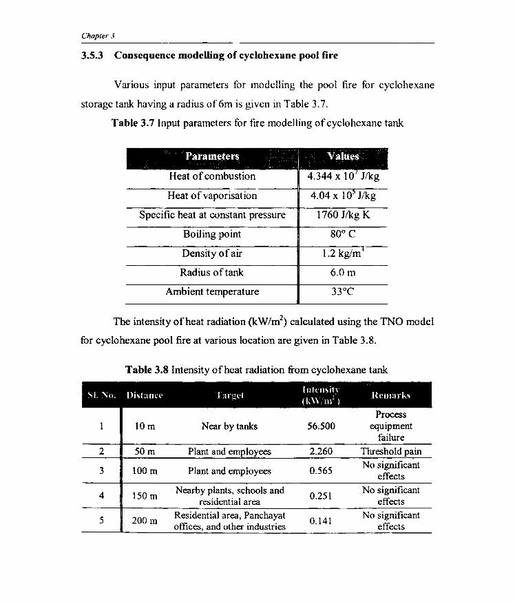
3.5.3 Consequence modelling of cyclohexane pool fire

Various input parameters for modelling the pool fire for cycIohexane

storage tank having a radius of6m is given in Table 3.7.

Table 3.7 Input parameters for tire modelling of cyclohcxane tank

Parameters ' i Values

Heat of combustion 4.344 x 10 J/kg

Heat of vaporisation 4.04 x 10' J/kg


Boiling point

Density of air 1.2 kglmJ

Radius of tank 6.0m

Ambient temperature


for cycIohexane pool fire at various location are given in Table 3.8.

Table 3.8 Intensity of heat radiation from cycIohexane tank

. lntl'Jl\ity SI. '\0. Dlslanct' I argl'j (I \\,:' Rt'llmrks

. ~ IUl I

Process 1 10m Near by tanks 56.500 equipment

failure

2 50m Plant and employees 2.260 Threshold pain

3 lOOm Plant and employees 0.565 No significant

effects

4 150m Nearby plants, schools and

0.251 No significant

residential area effects

5 200 m Residential area, Panchayat 0.141

No significant offices, and other industries effects

Consequence modelling o/hazardous -'fOrages

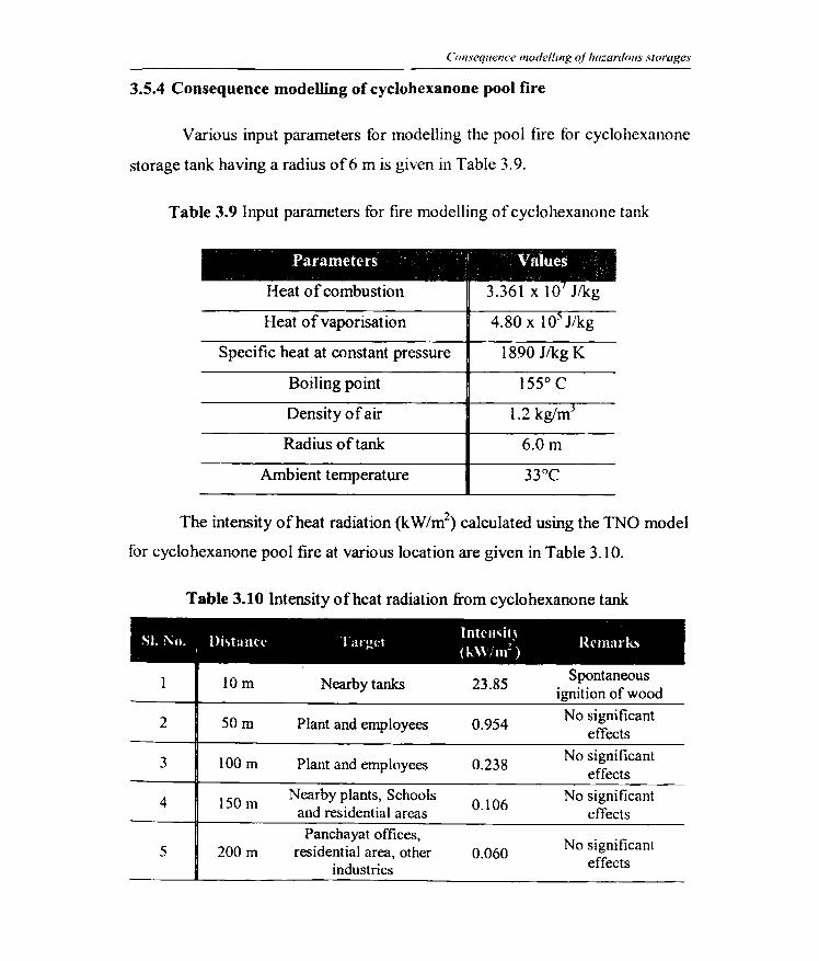
3.5.4 Consequence modelling of cyclohexanone pool fire

Various input parameters for modelling the pool tire for cyclohexanone

storage tank having a radius of6 m is given in Table 3.9.

Table 3.9 Input parameters tor fire modelling of cycIohexanone tank

Parameters I Values -

Heat of combustIon 3.361 x 10 J/kg

Heat of vaporisation 4.80 x 10' J/kg


Boiling point 1550 C

Density of air 1.2 kglmj

Radius of tank 6.0m

Ambient temperature


for cyclohexanone pool fire at various location are given in Table 3.10.

Table 3.10 Intensity of heat radiation from cyclohexanone tank.

. . Intcllsil\ SI. 1'0. Dlo,tann' I argl't " Ih'marks

I (k\\/m-)

IOm Nearby tanks 23.85 Spontaneous

ignition of wood


effects

3 100 m Plant and employees 0.238 No significant

effects

4 150 m Nearby plants, Schools


and residential areas effects Panchayat offices,

No significant 5 200 m residential area, other 0.060 industries effects

Chapter 3

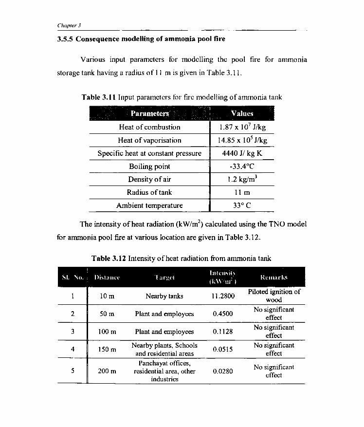
3.5.5 Consequence modelling of ammonia pool fire

Various input parameters for modelling the pool fire for ammoma

storage tank having a radius of II m is given in Table 3.11.

Table 3.11 Input parameters for fire modelling of ammonia tank

I

Parameters I Values I

Heat of combustion 1.87 X 107 J/kg

Heat ofvaporisation 14.85 x 105 J/kg

Specific heat at constant pressure 4440 J/ kg K

Boiling point

Density of air

Radius of tank llm

Ambient temperature


for ammonia pool fire at various location are given in Table 3.12.

Table 3.12 Intensity ofheat radiation from ammonia tank

I • • Inlellsih SI. .'\0. Ill\talll.'l' I ar~tt k\\~' Remark,

( . III )

10m Nearby tanks 11.2800 Piloted ignition of

wood


effect

3 100 m Plant and employees 0.1128 No significant

effect

4 150 m Nearby plants, Schools


and residential areas effect

Panchayat offices, No significant 5 200 m residential area, other 0.0280

industries effect


3.5.6 Consequence modelling of naphtha pool fire

Various input parameters for modelling the pool fire for naphtha storage

tank having a radius of 6 m is given in Table 3.13.

Table 3.13 Input parameters for fire modelling of naphtha tank

Parameters I Values I

Heat of Combustion

Heat of vaporisation 3.02 x 105 J/kg


Boiling point

Density of air 1.2 kg/m3

Radius of tank 6m

Ambient temperature


for naphtha pool tire at various location are given in Table 3.14.

Table 3.14 Intensity of heat radiation from naphtha tank

SI. No. Distance Target Intensity Remarks

tOm No important things 41.00 Failure of process equipments

2 50m Plant and

1.60 No significant

employees etTects

3 lOOm Plant and

0.40 No significant

employees etTects

4 150m Phmt and 0.18

No significant employees effects

5 200 m Public places 0.10 No significant effects

Chapter j

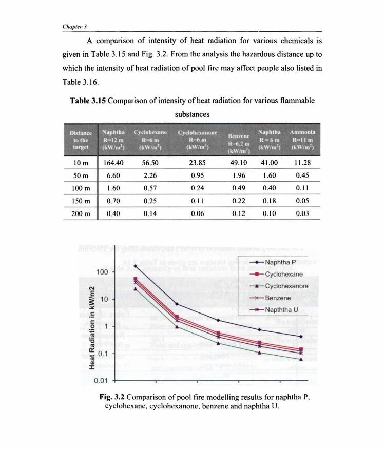
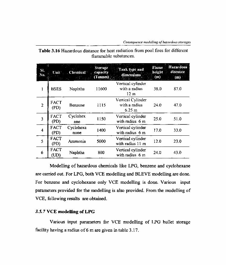
A companson of intensity of heat radiation for various chemicals is

given in Table 3. 15 and Fig. 3.2. From the analysis the hazardous distance up to

which the intensity of heat radiation of pool fire may affect people also listed in

Table 3.16.

Table 3.1S Comparison of intensity of heat radiation for various flammable

substances . '; - . .

Dislllncl.' ; Naphlha CHloheunc C,cJuhcununl.' R Nllphlhl ,\mmonill ., , • . erllene . lolbe . n~ 12m R "'bm ~' R" 6m.. , R = 6m R" II m

lurgel . ' (\;\\' /m!) : O.:\\Iml) , (""\- /m2) '; ~~.- ~ . (k\vlm~) 11.\\'/011) .~ .... ; ••. ~, •. : ... ,; ' •. ,,.-.,1, ( 101)

10m 164.40

50m 6.60

lOOm 1.60

150 m 0.70

200 m 0.40

100

N E ~ 10

c c o 1

"' M .., M

'" ... 0.1 M ~ J:

0.0 1

56.50

2.26

0.57

0.25

0.14

23.85 49.10 41.00 11.28

0.95 1.96 1.60 0.45

0.24 0.49 0.40 0. 11

0.11 0.22 0. 18 0.05

0.06 0.12 0.10 0.03

--+- Naphtha P

---Cyclohexane

-6-CycJohexanonE

""""*""" Benzene

- Napththa U

Fig. 3.2 Comparison ofpoollirc modelling resuhs for naphtha p, cycJohexane, cydohexanone. benzene and naphtha U.

Consequellce modelling of hazardous storages

Table 3.16 Hazardous distance for heat radiation from pool fires for different flammable substances.

I Storage T kt' d Flame Hazardous SI . an ~pe au h . I d' " ,tinit Chemical capacIty •. elg It lstance No. I (fonnes)" dimcu$.lons, (m) (m)

2

3

4

5

6

I _ , , • ,

BSES Naphtha

FACT Benzene (PD)

FACT Cyclohex (PD) ane

FACT Cyc10hexa (PD) none

FACT Ammonia (PD)

FACT Naphtha

(UD)

11600

1115

1150

1400

5000

800

Vertical cylinder with a radius

12 m

Vertical Cylinder with a radius

6.25 m

Vertical cylinder with radius 6 m




38.0 87.0

24.0 47.0

25.0 51.0

17.0 33.0

12.0 23.0

24.0 43.0

Modelling of hazardous chemicals like LPG, benzene and cyc10hexane

are carried out. For LPG, both VCE modelling and BLEVE modelling are done.

For benzene and cycIohexane only VCE modelling is done. Various input

parameters provided for the modelling is also provided. From the modelling of

VCE, following results are obtained.

3.5.7 VCE modelling of LPG

Various input parameters for VCE modelling of LPG bullet storage

facility having a radius of6 m are given in table 3.17.

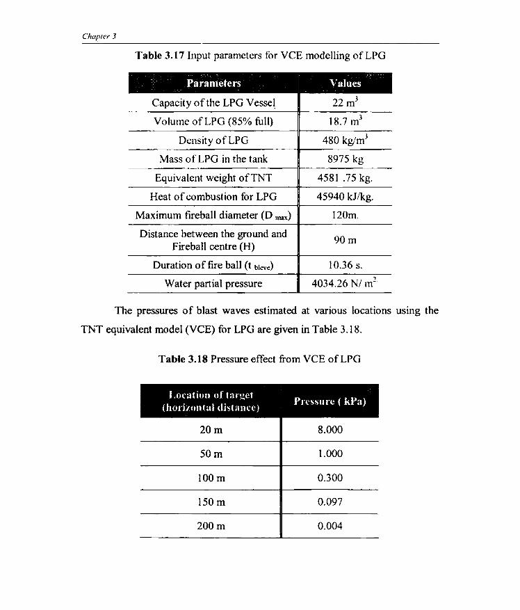
Chapter 3

Table 3.17 Input parameters for VCE modelling of LPG

Parameters Values

Capacity ofthe LPG Vesse~ 22 m3

Volume ofLPG (85% full) 18.7 m3

Density ofLPG 480 kg/m3

Mass of LPG in the tank 8975 kg

Equivalent weight of TNT 4581 .75 kg.

Heat of combustion for LPG 45940 kJ/kg.

Maximum fireball diameter (D max) 120m.

Distance between the ground and 90m Fireball centre (H)

Duration of fire ball (t him) 10.36 s.

Water partial pressure 4034.26 NI m2

The pressures of blast waves estimated at various locations using the

TNT equivalent model (VCE) for LPG are given in Table 3.18.

Table 3.18 Pressure effect from VCE ofLPG

Location of tar~ct P kP . .' rcssu re ( a) (honzontal distance)

20m 8.000

50m 1.000

lOOm 0.300

150 m 0.097

200 m 0.004

Cunsequence modellil/g uOwzllrdous slOrllges

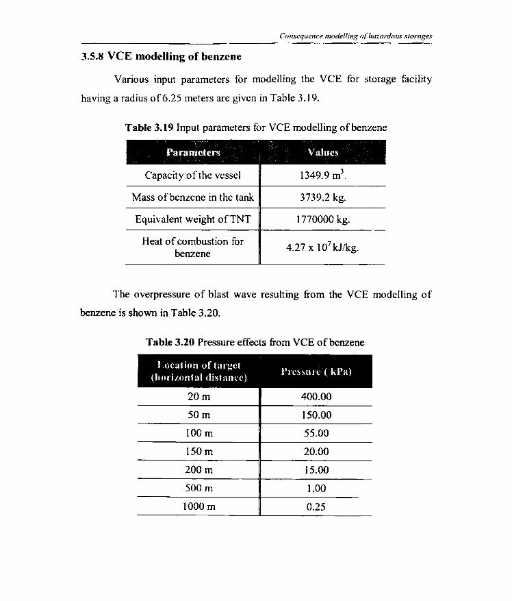
3.5.8 VCE modelling of benzene

Various input parameters for modelling the VCE for storage facility

having a radius of6.25 meters are given in Table 3.19.

Table 3.19 Input parameters for VCE modelling of benzene

Parameters : Values

Capacity of the vessel

Mass ofbenzene in the tank

Equivalent weight of TNT

Heat of combustion for benzene

3739.2 kg.

1770000 kg.

4.27 x 107 kJlkg.

The overpressure of blast wave resulting from the VCE modelling of

benzene is shown in Table 3.20.

Table 3.20 Pressure effects from VCE of benzene

Location of targN P kl) . . ' n.'SStHl' ( a) (hof'lLontai (listanc{')

20m 400.00

50m 150.00

lOOm 55.00

150m 20.00

200 m 15.00

500 m 1.00

1000 m 0.25

Chapter 3

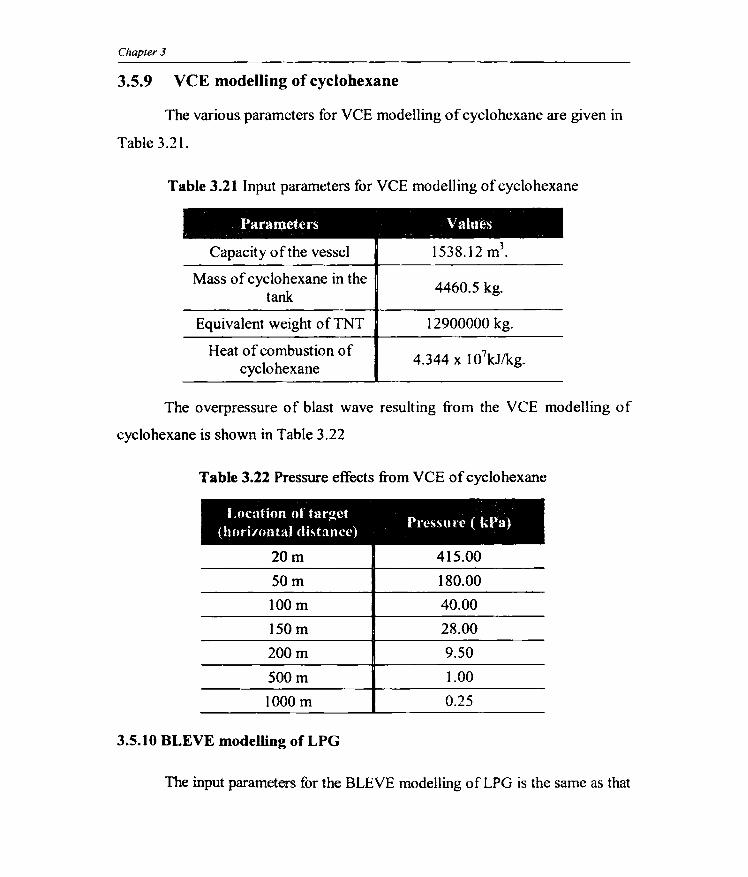
3.5.9 VCE modelling of cyclohexane

The various parameters for VCE modelling of cyclohexane are given in

Table 3.21.

Table 3.21 Input parameters for VCE modelling ofcyclohexane

Parameters Values

Capacity of the vessel

Mass of cyclohexane in the tank

Equivalent weight of TNT

Heat of combustion of cyclohexane

4460.5 kg.

12900000 kg.

4.344 x 107kJlkg.

The overpressure of blast wave resulting from the VCE modelling of

cyclohexane is shown in Table 3.22

Table 3.22 Pressure effects from VCE of cyclohexane

I,ocation of target p - kP ) ., n~ssur(' ( a (horizontal <hstanc(')

20m 415.00

50m 180.00

lOOm 40.00

150m 28.00

200 m 9.50

500 m 1.00

1000m 0.25

3.5.10 BLEVE modelling of LPG

The input parameters for the BLEVE modelling 0 f LPG is the same as that

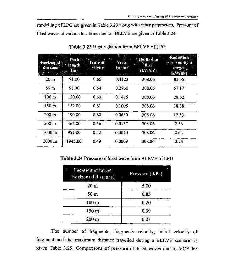
COl/sequence modelling of hazardolls storages

modelling ofLPG are given in Table 3.23 along with other parameters. Pressure of

blast waves at various locations due to BLEVE are given in Table 3.24.

Table 3.23 Heat radiation from BEL VE ofLPG

! -

Path Radiation Radiation

Horizontal I length Transmi View

flux received by a

distance (rn)

-ssivit;y l-actor (k\\/m2

) target ,

(kW/ni) .. -,' 20m 91.00 0.65 0.4123 308.06 82.55

50m 98.00 0.64 0.2960 308.06 57.17

100 m 120.00 0.63 0.1475 308.06 28.62

150 m 152.00 0.61 0.1005 308.06 18.88

200 m 190.00 0.60 0.0680 308.06 12.53

500 m 462.00 0.56 0.0137 308.06 2.36

1000 m 951.00 0.52 0.0040 308.06 0.64

2000 m 1945.00 0.49 0.0009 308.06 0.13

Table 3.24 Pressure of blast wave from BLEVE ofLPG

The

,

Location of targd Pressure ( kPa)

(horizontal dilitancc)

20m 5.00

50m 0.85

lOOm 0.20

150m 0.09

200 m 0.03

number of fragments, fragments velocity, initial velocity of

fragment and the maximum distance travelled during a BLEVE scenario is

given Table 3.25. Comparisons of pressure of blast waves due to VCE for

Chap/er 3

various chemicals are given in the Table 3.26. Comparisons are given in the

graphical fonn (Fig. 3.3) and the maximum threat zones for pressure waves are

given in the Table 3.27.

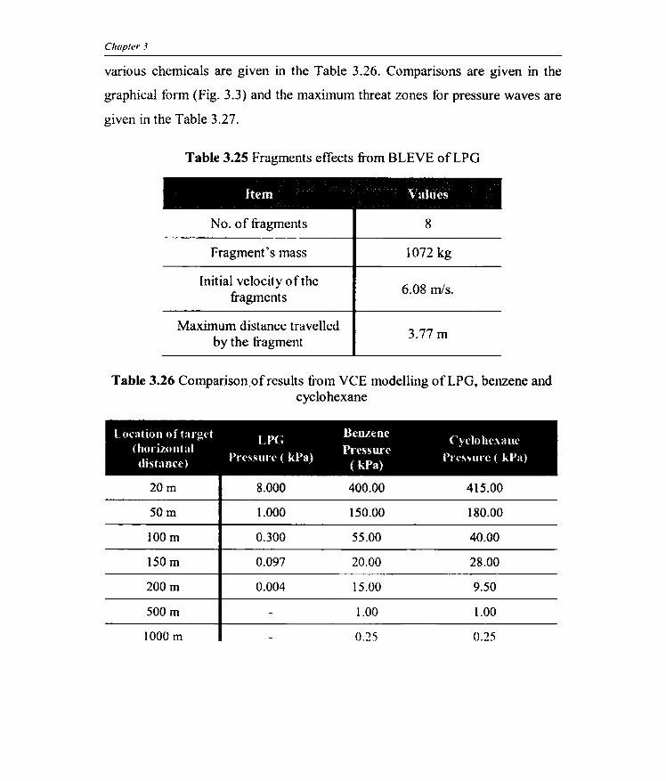
Table 3.25 Fragments effects from BLEVE ofLPG

Item V ~dlles

No. of fragments

Fragment's mass

Initial velocity of the fragments

Maximum distance travelled by the fragment

8

1072 kg

6.08 m1s.

3.77m

Table 3.26 Comparison.ofresults from VCE modelling ofLPG, benzene and cyclohexane

Location of target [ 1)(-' Beulene (' I I . , • vc () 1('\11nC

(horizontal Pressure' distance) Prc~~un' ( kPa) ( kl)a) Pn's~lIl'c ( kPlI)

20m 8.000 400.00 415.00

50m 1.000 150.00 180.00

lOOm 0.300 55.00 40.00

150m 0.097 20.00 28.00

200 m 0.004 15.00 9.50

500 m l.00 l.00

1000 m 0.25 0.25

2

3

Con.~eqUf!"Cf! mntiellinR nfhr:r.urUoU5 l ·IQrugn·

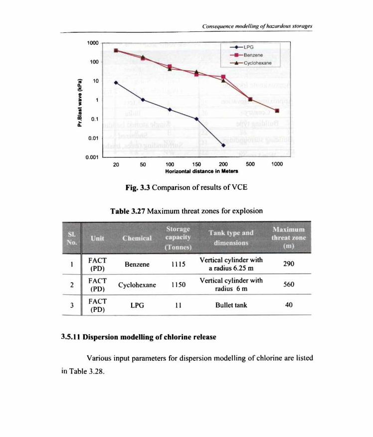
1000 ,-------------=--;;::~--, --+-- LPG ---........ 100 -r-Cydohexane

10 ----"'*'-..~

0.1

0.01

0.001 '--------------- - -------' 20 50 100 150 200 500 1000

Horizontal dlstan..- In V.r.rs

Fig. 3.3 Comparison of results of VCE

Table 3.27 Maximum threat zones for explosion

FACT Benzene 1115

Vertical cylinder with 290

(PO) a radius 6.25 m

FACT Cyclohexane 1150

Vertical cylinder with 560 (PO) radius 6 m

FACT LPG 11 Bullet tank 40

(PO)

3.5.11 Dispersion modelling of chlorine release

Various in put parameters for dispersion modell ing of chlo rine are li sted

in Table 3.28.

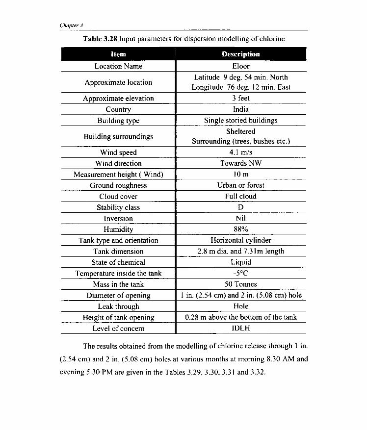
Chapter 3

Table 3.28 Input parameters for dispersion modelling of chlorine

Item I Description

Location Name Eloor

Approximate location Latitude 9 deg. 54 min. North

Longitude 76 deg. 12 min. East

Approximate elevation 3 feet

Country India

Building type Single storied buildings

Building surroundings Sheltered

Surrounding (trees, bushes etc.)

Wind speed 4.1 mls

Wind direction Towards NW

Measurement height ( Wind) IOm

Ground roughness Urban or forest

Cloud cover Full cloud

Stability class D

Inversion Nil

Humidity 88%

Tank type and orientation Horizontal cylinder

Tank dimension 2.8 m dia. and 7.31 m length

State of chemical Liquid

Temperature inside the tank -5°C

Mass in the tank 50 Tonnes

Diameter of opening I in. (2.54 cm) and 2 in. (5.08 cm) hole

Leak through Hole

Height of tank opening 0.28 m above the bottom of the tank

Level of concern IDLH

The results obtained from the modelling of chlorine release through I in.

(2.54 cm) and 2 in. (5.08 cm) holes at various months at morning 8.30 AM and

evening 5.30 PM are given in the Tables 3.29. 3.30, 3.31 and 3.32.

-


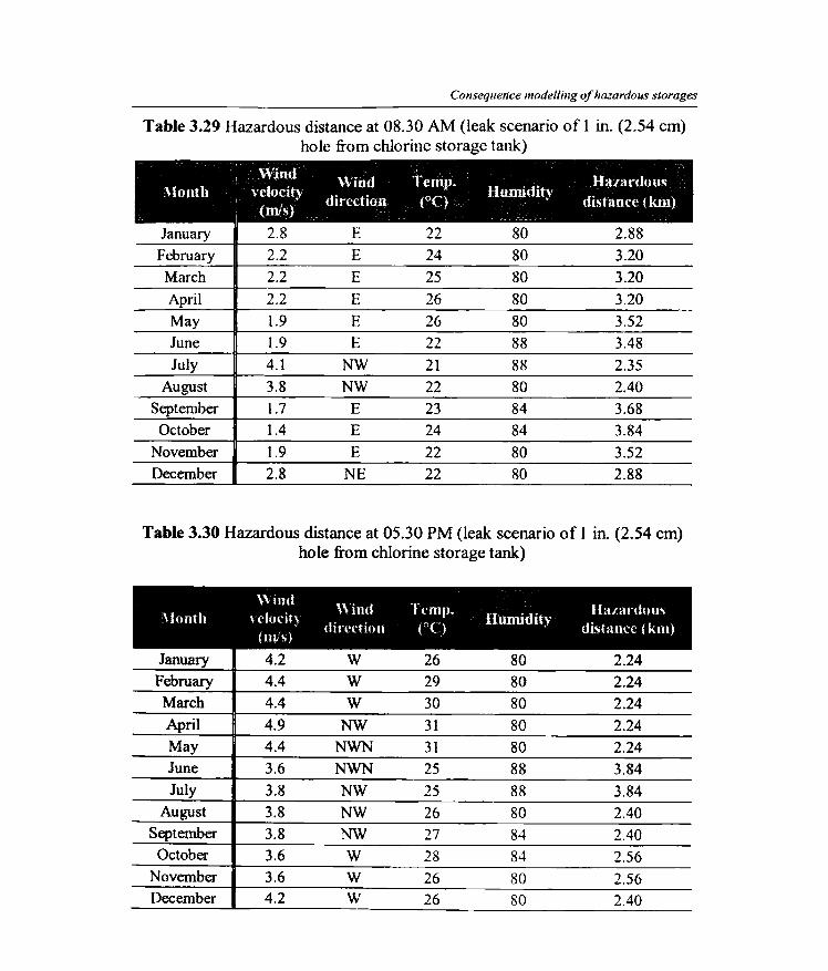
Table 3.29 Hazardous distance at 08.30 AM {leak scenario of 1 in. (2.54 cm) hole from chlorine storage tank)

Wind Wind Temp. Hazardous Month vclocit~, Humidity

(m/s) direction (OC) distance (km)

January 2.8 E 22 80 2.88 February 2.2 E 24 80 3.20

March 2.2 E 25 80 3.20 April 2.2 E 26 80 3.20 May 1.9 E 26 80 3.52 June 1.9 E 22 88 3.48 July 4.1 NW 21 88 2.35

August 3.8 NW 22 80 2.40 September 1.7 E 23 84 3.68

October 1.4 E 24 84 3.84 November 1.9 E 22 80 3.52 December 2.8 NE 22 80 2.88

Table 3.30 Hazardous distance at 05.30 PM (leak scenario of 1 in. (2.54 cm) hole from chlorine storage tank)

\\ind \\imt Tt·mp. Hazardous

~Ionth , docit~ Humidity (m/s)

direction (0(,) distance (km)

January 4.2 W 26 80 2.24 February 4.4 W 29 80 2.24

March 4.4 W 30 80 2.24 April 4.9 NW 31 80 2.24 May 4.4 NWN 31 80 2.24 June 3.6 NWN 25 88 3.84 July 3.8 NW 25 88 3.84

August 3.8 NW 26 80 2.40 September 3.8 NW 27 84 2.40

October 3.6 W 28 84 2.56 November 3.6 W 26 80 2.56 December 4.2 W 26 80 2.40

Chapter 3

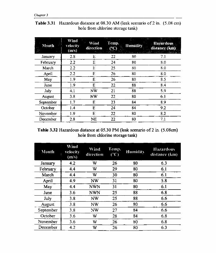
Table 3.31 Hazardous distance at 08.30 AM (leak scenario of2 in. (5.08 cm) hole from chlorine storage tank:)

I Wind Wind Temp. Hazardous Month velocitv lIumidity

! (m/s) direction (OC) distance (km)

, - ""'- .

January 2.8 E 22 80 7.1 February 2.2 E 24 80 8.0 March 2.2 E 25 80 8.0 April 2.2 E 26 80 8.0 May 1.9 E 26 80 8.5 June 1.9 E 22 88 8.4 July 4.1 NW 21 88 5.9



Table 3.32 Hazardous distance at 05.30 PM (leak scenario of2 in. (5.08cm) hole from chlorine storage tank)

'''iutl " ind Tt'mp. 11 aL~ll'd()us

'Iouth vdocity l1ul11idit:" (m/s)

direction (oC) di<.tanct.' (km)





Consequence modelling of hazardo/ls storages

3.5.12 Dispersion modelling of ammonia release

Input parameters for dispersion modelling of ammonia are given in the

Table 3.33.

Table 3.33 Input parameters for dispersion modelling of ammonia

Item i Description I Location Name Eloor

Approximate location Latitude 9 deg. 54 min. North

Longitude 76 deg. 12 min. East Approximate elevation 3 feet

Country India Building type Single storied buildings

Building surroundings Sheltered

Surrounding (trees. bushes etc.) Wind speed 4.1 m1s

Wind direction Towards NW Measurement height

IOm (Wind)

Ground roughness Urban or forest Cloud cover Full cloud

Stability class D Inversion Nil Humidity 88%

Tank type and orientation Vertical cylinder Tank dimension 22 m dia. and 20.77 m len~h State of chemical Liquid

Temperature inside the tank -33.2°C Mass in the tank 5000 Tonnes

Diameter of opening 1 in. (2.54 cm) • 2 in (5.08 cm) and 5 in.

12.7 cm)in. Leak through Hole

Height of tank opcning 2.1 m above the bottom of the tank Level of concern IDLH

Hazardous distance at various leak scenarios such as leaks from 1 inch,

2 inches and 5 inches are obtained from the dispersion modelling and are

Chapter 3

Table 3.34 Hazardous distance at 08.30 AM (leak scenario of 1 in. (2.54cm) hole from ammonia storage tank)

! Wind "

, Wind Temp. Hazardous Month ! \clocity

direction ee) Humidity distap'ce . (km)

(m')!) . ~ ~ ~'

f'~ '-' ' I,.L':;;' -",""





Table 3.35 Hazardous distance at 05.30 PM (leak scenario of 1 in. (2.54 cm) hole from ammonia storage tank)

,

! Wind \\ ind 'Il'mp. Ila.lardolls

'-looth ; \'clucit~ din'ction eC) Hllmidity

distanCt' l km) (nn)





Consequence modelling a/hazardolls slOrages

Table 3.36 Hazardous distance at 08.30 AM (leak scenario of2 in. (5.08cm) hole from ammonia storage tank)

Month Wind velocit) \Vind Temp.

Humidity Hazardous (m/s) direction ee) distance (km)

:





Table 3.37 Hazardous distance at 05.30 PM (leak scenario of 2 in. hole from ammonia storage tank)

Wind Wind I Clllp. Ha.tardous

\lonth velocity I1l1f11idit~ (mJs)

direction ({') distance (km)





Chapter 3

Table 3.38 Hazardous distance at 08.30 AM (leak scenario of 5 in. hole from ammonia storage tank)

;\Ionth \Vind velocit)· Wind Temp.

Humidit)· Hazardous (m!s) dircdion (OC) distance O<m)

January 2.8 E 22 80 4.19 February 2.2 E 24 80 4.51 March 2.2 E 25 80 4.51 April 2.2 E 26 80 4.51 May 1.9 E 26 80 4.83 June 1.9 E 22 88 4.67 July 4.1 NW 21 88 3.70



Table 3.39 Hazardous distance at 05.30 PM (leak scenario of5 in. (12.7 cm) hole from ammonia storage tank)

\\ ind \\ in£! I',.'mp. Ila/ardolls

\Ionth \dodt~ 1It1lllidi(~

(rn's) din'clion (cC) distancl' (km)

January 4.2 W 26 80 3.54 February 4.4 W 29 80 3.54 March 4.4 W 30 80 3.54 April 4.9 NW 31 80 3.38 May 4.4 NWN 31 80 3.54 June 3.6 NWN 25 88 3.86 July 3.8 NW 25 88 3.86



Conseqllence modeilillg 0/ hazardolls storages

3.5.13 Dispersion modelling of benzene release

Input parameters for dispersion modelling of benzene are given in Table

3.40.

Table 3.40 Input parameters for dispersion modelling of benzene - , - ~ ~o;- ... =~

Item Des~ripijon " , I • ~ > ...

Location Name Eloor

Approximate location Latitude 9 deg. 54 min. North Longitude 76 deg. 12 min. East

Approximate elevation 3 feet

Country India

Building type Single storied buildings

Building surroundings Sheltered Surrounding (trees, bushes etc.)

Wind speed 4.1 mls

Wind direction Towards NW

Measurement height ( Wind) lOm

Ground roughness Urban or forest , Cloud cover Full cloud

Stability class D

Inversion Nil

Humidity 88%

Tank type and orientation Vertical cylinder

Tank dimension 12. 5 m dia. and 11 m length

State of chemical Liquid

Temperature inside the tank 30°C

Mass in the tank 1115 Tonnes

Diameter of opening 1 in. (2.54 cm) , 2 in (5.08 cm) and 5 in. (12.7 cm)

Leak through Hole

Height of tank opening I. I m above the bottom of the tank

Level of concern IDLH

Hazardous distance at various leak scenarios such as leaks from 1 in., 2

111., and 5 in. holes are obtained from the dispersion modelling and are

presented in the Tables 3.41,3.42,3.43,3.44,3.45 and 3.36.

Chapter 3

Table 3.41 Hazardous distance at 08.30 AM (leak scenario of 1 in. (2.54 cm) hole from benzene storage tank)

\Vind \Yind Temp. Ha7.Jlrdous Month wlocit)- Humidity

! (m/s) direction (0C) distance (m)

January 2.8 E 22 80 58 February 2.2 E 24 80 71

March 2.2 E 25 80 71 April 2.2 E 26 80 70 May 1.9 E 26 80 73 June 1.9 E 22 88 73 July 4.1 NW 21 88 46

August 3.8 NW 22 80 48 September 1.7 E 23 84 75

October 1.4 E 24 84 78 November 1.9 E 22 80 73 December 2.8 NE 22 80 58

Table 3.42 Hazardous distance at 05.30 PM (leak scenario of 1 in. (2.54 cm) hole from benzene storage tank)

Wind " ind '1 Cfilp. I [umidit Ila/ardoll'

i\louth .. clocity (ms)

direction ('C) ~ dhtancc (m)

January 4.2 W 26 80 48 February 4.4 W 29 80 48 March 4.4 W 30 80 49 April 4.9 NW 31 80 46 May 4.4 NWN 31 80 49 June 3.6 NWN 25 88 51 July 3.8 NW 25 88 51

August 3.8 NW 26 80 51 September 3.8 NW 27 84 51

October 3.6 W 28 84 53 November 3.6 W 26 80 53 December 4.2 W 26 80 48

Consequence modelfillg a/hazardous slorages

Table 3.43 Hazardous distance at 08.30 AM (leak scenario of2 in. (5.08 cm) hole from benzene storage tank

Wind Wind Temp. Hazardous

Month I \ ,'Iocity Humidity

I (m/s) direction (0C) distance (ml

January 2.8 E 22 80 135 February 2.2 E 24 80 144

March 2.2 E 25 80 144 April 2.2 E 26 80 144 May 1.9 E 26 80 149 June 1.9 E 22 88 148 July 4.1 NW 21 88 95

August 3.8 NW 22 80 101 September l.7 E 23 84 152


Table 3.44 Hazardous distance at 05.30 PM (leak scenario of2 in. (5.08 cm) hole from benzene storage tank)

Wind \\ ind "1l'lIlp. Hazanious

i\lomb H'locit) di rl'l't iOIl ('C)

Jlumjdit~ dista Ill'l' (Ill) (mo',)

January 4.2 W 26 80 99 February 4.4 W 29 80 99

March 4.4 W 30 80 101 April 4.9 NW 31 80 95 May 4.4 NWN 31 80 101 June 3.6 NWN 25 88 123 July 3.8 NW 25 88 104



Chapter J

Table 3.45 Hazardous distance at 08.30 AM (leak scenario of5 in. (l2.7 cm) hole from benzene storage tank)

\Vind Wind Temp. lIumidit Ilazardous Month vl'locity

direction (OC) dista nee (m) (m/s)

y

January 2.8 E 22 80 355 February 2.2 E 24 80 401 March 2.2 E 25 80 405 April 2.2 E 26 80 400 May 1.9 E 26 80 428 June 1.9 E 22 88 314 July 4.1 NW 21 88 321

August 3.8 NW 22 80 323 September 1.7 E 23 84 427


Table 3.46 Hazardous distance at 05.30 PM (leak scenario of5 in. (12.7cm) hole from benzene storage tank)

Wind \\ind rl'mp Ilazarduus

i\lonth \docit~ Illlmidit~

t 1111's) direction (0C) dhtamx' (m)

January 4.2 W 26 80 315 February 4.4 W 29 80 316

March 4.4 W 30 80 318 April 4.9 NW 31 80 306 May 4.4 NWN 31 80 320 June 3.6 NWN 25 88 321 July 3.8 NW 25 88 328



Conseqllence modelling of hazardous storages

Hazardous distances for chlorine, ammonia and benzene are compared in the

Tables 3.47 and 3.48.

Table 3.47 Hazardous distance in kilometers at 08.30 AM for ammonia, chlorine and benzene

January 1.41 1.77 2.88 9.0 0.058 0.135

February 1.53 1.77 3.20 9.2 0.071 0.144

March 1.54 1.77 3.20 9.2 0.071 0.144

April 1.54 1.77 3.20 9.2 0.070 0.144

May 1.61 1.93 3.52 8.6 0.073 0.149

June 1.61 1.93 4.48 8.6 0.073 0.148

July 1.07 1.61 3.52 8.6 0.046 0.095

August 1.08 1.61 2.40 9.0 0.048 0.101

September 1.32 1.93 3.68 8.5 0.075 0.152

October 1.44 2.09 3.84 8.1 0.078 0.158

November 1.27 1.93 3.52 8.6 0.073 0.147

December 1.14 1.77 2.88 9.0 0.058 0.135

Chapler 3

Table 3.48 Hazardous distance in kilometers at 05.30 PM for ammonia, chlorine and benzene

JanualY 1.07 1.77 2.4 9.0 0.048 0.099

February 1.07 1.77 2.24 9.0 0.048 0.099

March 1.07 1.77 2.24 9.0 0.049 0.101

April 1.06 1.77 2.24 9.0 0.046 0.095

May 1.07 1.93 2.24 9.0 0.049 0.101

June 1.09 1.93 3.84 9.0 0.051 0.123

July 1.08 1.61 2.84 9.0 0.051 0.104

August 1.08 1.61 2.40 9.0 0.051 0.104

September 1.09 1.93 2.40 9.0 0.051 0.106

October 1.10 2.09 2.56 9.2 0.053 0.123

November 1.09 1.93 2.56 9.0 0.053 0.123

December 1.07 1.77 2.40 9.0 0.048 0.099

Table 3.49 Maximum threat zone and direction of toxic gas release for different chemicals

I Hazardous di'it!lIH.'{· and lIazardou .. ~istance and I

: din'ction for rdras(' from I din'ction for release fl'om 2 in. Chemical i in. (2.54 cm) hole (S.08 cm)bole

Chlorine

Ammonia

Benzene

I iUO AM 5.30 P\l S.30 AM 5.30 PM

4.480 km E

1.610 km E

0.078 km E

3.840 km NW

1.100 km W

0.053 km W

9.200 km E 9.200 km W

2.090 km E 2.090 km W

0.158 km E 0.123 km W

Consequence modelling of hazardous slOrages

The intensity of the heat radiation resulting from pool fIres at various

locations is estimated. A comparison of intensity of heat radiation at various

locations is given in Table 3.15 and Fig. 3.2 for various chemicals, The intensity of

heat radiation is the maximum at 10 meters from the source of pool tIrC for all the

chemicals. A naphtha pool fire having a radius of 12 meters is found to have

maximum intensity of heat radiation. This is mainly due to the large radius of the

storage tank and comparatively high heat of combustion and heat of vaporization

values of naphtha. For ammonia, even though the radius of the tank is large, the

intensity of heat radiation is less. This is mainly because of the low heat of

combustion and heat of vaporization values of ammonia. The hazardous distances

up to which the heat radiation of pool fIre may affect people are listed in Table

3.16. The various effects of pressure waves are given in Table 3.2. A comparison

of pressure of blast waves due to VCE for various chemicals is given in the Table

3.26. From this table it is observed that the pressure of a blast wave is very less for

LPG and high for cyclohexane. This may be attnbuted to the to less storage

quantity ~f LPG and its lower heat of combustion values. However, the

corresponding values for benzene and cyclohexane are fuund to be high. It is also

observed that the pressure of blast wave due to VCE is higher than that of the

BLEVE (Table 3.24). This is because some amount of energy of the explosion is

utilized for the fragmentation of the vessel and its missile effects. Comparison is

given in the graphical form (Fig. 3.3). The maximum threat zones for pressure

waves resulting from the VCE of various chemicals are given in Table 3.27. The

results of ALOHA air modelling for chlorine, ammonia and benzcne are given in

the Tables 3.47 & 3.48 for various leaks scenarios. It is observed that the threat

zones are the maximum for chlorine, for both morning and evening and it is around

9.2 kilometers for a leak scenario for a 2-inch hole. The maximum threat zones for

various chemicals and its direction are given in Table 3.49. These results will give

us a clear picture of the hazard potential ofthese storages. Estimation ofthe hazard

Chapter 3

potential is the first step in any disaster management plan. The results obtained

from the above analysis will also provide guidelines for land use planning in the

areas surrounding the MAH industries.

3.6 CONCLUSIONS

Consequence analysis IS gammg importance Il1 the industrial disaster

mitigation and management decisions. The present study shows that industries

having bulk storages of hazardous chemicals could pose a high potential for

damage to those inside and outside the industry. Fire modelling shows that the

hazardous distances t()r certain chemicals extended up to 90 meters which

might prevent effective fire flghting in case of a pool fire. The domino effects

on adjacent tanks are also found to be significant in many cases. Consequence

analysis results should be taken in to account while deciding the distance

between the tanks. The consequence calculations have been made ti:>r explosion

scenarios also. A maximum threat zone of 560 meters is observed in the case of

cyclohexane. This may be due to the highly explosive nature of cyclohexane.

This tIu-eat zone can be shortened by reducing the inventory of cyclohexane. It

is observed that as the wind velocity increases, threat zone distance decreases.

As the wind speed increases, the material is carried down by the wind faster,

but the material is also diluted faster by a large quantity of air [8]. So when

wind velocity increases, even though we expect a large threat zone, we will get

only a smaller threat zone with specific level of concern because of the dilution

of the cloud with air. But as the temperature increases threat zone distance

increases. But the low temperature variation doesn't have much influence on

the threat zone. Dispersion modelling results and the wind direction t()r a

particular period, can greatly improve emergency preparedness and can be

powerful decision making tools for locating rehabilitation centres and the local

emergency control rooms.

CO/lseqllence II/odelling of hazardous storages

References

[1] OGP data base, Risk assessment data report No 434-7,Consequencc

modelling, International Association of Oil and Gas Producers, 20 10.

[2] F.l. Khan and S.I\. Abbasi, A criterion t<')r developing credible

accident scenarios t()r risk assessment, J. Loss Prev. Process Imf. 15

(2002) 467-475.

[3] Health Safety Executive, An independent review ofHSE methodology

for assessing societal risk, IIChE, 2006.

[4] A.E. Cots, Fire protection hand book. eighteenth cd., NFPA, Quincy,

1997.

[5] F.P. Lees, Loss prevention in process industries, YoU, second ed.,

Buttcrworth & Heinemann, UK, 1996.

[6] F.E. Mc Elory, Accident prevention manual for cngmeenng and

technology, 12th ed., NSC, USA, 2001.

[7] V.K, lain, Fire Safety in Buildings, New Age International (P) Ltd.,

New Delhi, 1996.

[8] AIChE/CCPS, Guideline for chemical process quantitative risk

analysis, second cd., New York, 2000.

[9] ILO-NSC, Major hazard control- a practical manual, International

Labor office, Geneva, 1996.

[10] R. Hirst, Underdowns practical fire precautions, Gower publishing

company Ltd., England, 1989.

[11] Manual of firemanship, Book No.l, second ed., HMSO, London

(1990).

Chaplcr 3

[12] AIChE/CCPS, Guideline for evaluating the characteristics of vapour

cloud explosions, flash fire and BLEVE, New York, 1994.

[13] D.A. Crowl and J.F. Louvar, Chemical process safety; Fundamentals

with application, Prentice Hall, New Jersey, 1990. (ISBN 0-13-12970)

[14] NFPA 69, Explosion prevention systems Quincy, MA, NFPA.

[15] L.J. Cralley, L.V. Cralley, Patty's industrial hygiene and toxicology

VoU, second ed., John Wilcy & Sons, New York, 2000.

[161 Manutaeture storage and import of hazardous chemicals (MSIHC)

Rules, India, 1989.

[17] The Chemical accidents (Emergency planning, preparedness, and

response) Rules, India, 1996.

[18] World Bank, Technique for assessmg industrial hazards, Technical

Paper No.55, A manual, Technica Ltd., 1988.

[19] G. Madhu, Modelling of pool tires, J. of Fire Eng. 1 (2002) 1-10.

[20] ALOHA 5.2.3 package - Environmental Protection Agency, USA.

[21] Robert H. Perry , Don W. Green, Perry's Chemical Engineers

Handbook, seventh ed., Mc Graw Hill, New York, 1997.

[22] W.L. Nelson, Petroleum refinery engineering, t()urth cd., Mc Graw Hill,

1958.

[23] CAMEO 1.2.1 package - Environmental Protection Agency, USA.

[24] Mudan, Thermal radiation hazards ti'om large pool fires and fIre balls

Process Energy Combust. Science, 10 (I) (1984) 59- RO.

COllsequence modelling of hazardous :i(orages

[25] TNO, Method for the calculation of physical effects of the escape of

dangerous materials: liquids and gases (the yellow book), The

Netherlands organization t()r applied scientific research, Apcldoonn,

the Netherlands, 1979.

[26] G. Hcskestad, Engineering relations t()[ fire plumes, Fire Sarety

Journal, (1984), 25-32.

[27] Q.A. Baker, P.A. Cox, P.S. Westive, J.J. Kulcsc, Explosion hazards

and evaluation, Elsevicr, New York, 1983.

[28] Dccker, An analytical method for estimating overprcssure form

theoretical atmospheric explosions, NFP A annual meeting,

Quency, NFP A 1974.

[29] W.P.M Merex, A.C Van den Berg, and CJ. lIayhurst. Developments

in vapour cloud explosion blast modelling, J. Haz. Mater. 71 (2000)

301-319.

[30] w.e. Braise and D.W. Simpson, Guidelines for estimating

damage explosions. 22nd Loss prevention sympOSIum. CEP

Technical manual, New York. AIChE. 1968.

[31] Health Safety Executive, Advisory committee on major hazards:

Second report, London HMSO (ISBN 0-4713-7108-4) 1979.

[32] Health Safety executive, The effects of explosion in the process

Industries, Loss prevention bulletin, 68 (1986) 37-47.

[33] Industrial Risk Insurers, Oil and chemical properties loss potential

estimation guide; IRI information, 1990 ..

[34] Factory Mutual Research Corporation, private communication

1990, (CCPS 1994).

Chapter 3

[35] E. Planas Cuchi, 1.M. Salla and 1. Casal, "Calculating Overpressure from

BLEVE explosions' 1. Loss Prey. Process Ind. 17 (2004) 431-436.

[36] J.M. Salla, M. Demichela, and J. Casal ,BLEVE: A new approach to

the super heat limit temperature'. J. Loss Prey. Process Ind. 19 (2006)

690-700.

[37] W.L. Walls, The BLEVE - part 1 . Fire Command, 1979.

[38] A.F. Robel1s, Thc1111al radiation hazards from release of LPG ft'om

pressurized storage, Fire Safety Journal 3, (1981) 197-212.

[39] Hymcs, The physiological and pathological effects of thermal

radiation, SRD R 275, Atomic Energy Regulatory Authority, UK,

1981.

[40] Pietersen, Huerta, , Analysis of the LPG incident in San Juan

Ixhuattepec, Mexico city, TNO 84-022, Netherlands Organization for

applied scientific researches, 1985.

[41] Mudan, Corce, Fire hazards calculation for large open hydrocarbon

fires, SFPE Handbook, Society of Fire Protection Engineers, Boston,

1988.

[42] Angas Sengupta, AK. Gupta, and I.M. Mishra, Layout of fuel tanks in

a tank farm, Loss Prey. Process Ind. (20lO) 1-7.

[43] R.M. Pitblado, Consequence modeling for BLEVE incidents : Major

Industrial Hazards project. Technical papers, Sydney, Australia.

University of Sydney ( ISBN 0-949269-37-9) 1986.

[44] Tasnecm Abbasi, S. A. Abhasi , The boiling liquid expanding vapor

explosion (BLEVE): mechanism consequence assessment,

management J. Haz. Mater. 141 (2007) 489-519.

Consequellce lIIodelllllg of hazard OilS slorages

[45] Holden, Reeves, Fragment hazards from failure of pressurized

liquefied gas vessels; Assessment and control of major hazards, IChE

Sym. Ser No.93. (1985) 205-20.

[46] 1. Stawczyk, Experimental evaluation of LPC; tank explosion hazards.

J. Haz. Mat. B 96 (2003) J g9-200.

[471 Brown, Energy release protediol1 f{)r pressurized systems, part I,

review of studies into blast and fragmentation, Appl. Mech. rev. 38

(12)( 1985) 1625-51.

[48] Moorce, The design 0 f barricades t(Jr hazardous pressure systems,

Nuclear Engineering Design 5 (1967) 1550-66

[49] M.R. Baum, 1. Pressure Vessel Technology (1988) 168-176.

[50] R.W. Prug, Quantitative evaluation of BLEVE hazards. 2211<1 loss

prevention symposium, AIChE, New York, 1988.

[51] C.S. Rao, Environmental pollution control engineering, New age

international, New Delhi, 2003.

[52] S.R. Hanna, D.G. Strimaitus, J. Chang, Result of hazard response

model evaluation using desert tortoise and gold fish database, Vol.l,

API, Washington DC ,1990.

[53] API, Hazard response modelling uncertainty; Evaluation of

commonly used hazardous dispersion models, API publication,

Washington DC, 1992.

[54J S.R. Hanna, G.A. Briggs, R.P. Hosker, Hand book on ditfusion. Oak

Ridge, USA, 1982.

[55] F. Pasqill, F.B. Smith, Atmospheric diffusion, third ed. Halsted, New

York, 1983.

Chapter 3

[56] Y. 1chikawa, K. Sada, A method of evaluating the topographical eftect

on atmospheric dispersion using a numerical model International J.

Env. Pollution 16 (1-6) (2010) 439-450.

[57] Tom Spicer and Jerry Havens; Users guide tor the DEGAD1S dense

gas dispersion, Ot1icc of air quality planning and standards, LJSEPA,

19!.N.

[58] Wind Roses tC)f Cochin City (1976-90), India meteorological

Department.

[59] U.S. Environmental protection Agency, ALOHA user's manual 2007 .

........ r>l1£o ......

Documents

CONSEQUENCE MODELLING OF HAZARDOUS STORAGES