Embed Size (px)
Citation preview

Confidential
Final Report
Contract # 029 of 2013 Version 1.2
Developing the Methodology for Calculation of the Firm Energy of a
Geothermal Power Plant
Submitted by: Warren T. Dewhurst, Ph.D., .P.E. Grupo Dewhurst, SAS Carrera 28 D #68-42 Manizales, Caldas Colombia [email protected] www.dewhurstgroup.us December 19, 2013
Submitted to: Mr. Javier Augusto Díaz Velasco
Experto Comisionado Comisión de Regulación de Energía y Gas - Av. Calle 116 No. 7-15. Edificio Cusezar, int
2, oficina 901 Bogota, Colombia [email protected]
Comisión de Regulación de Energía y Gas (CREG)

CONFIDENTIAL
2 | CREG Contract #029 of 2013
INTENTIONAL BLANK PAGE

CONFIDENTIAL
3 | CREG Contract #029 of 2013
Contents Introduction .................................................................................................................................................... 5
Objective ..................................................................................................................................................... 5
Report Content ........................................................................................................................................... 5
Background ..................................................................................................................................................... 5
Reservoir Characteristics ............................................................................................................................ 6
Permeability, Enthalpy, and Temperature.............................................................................................. 6
Solids ....................................................................................................................................................... 7
Gathering Systems ...................................................................................................................................... 7
Power Plant Cycle Types ............................................................................................................................. 7
Binary (Air Cooled) .................................................................................................................................. 7
Binary (Water Cooled) ............................................................................................................................ 9
Flash (Water Cooled) .............................................................................................................................. 9
Phases of a Geothermal Project ............................................................................................................... 11
Methodology ................................................................................................................................................ 14
Design Point Output ................................................................................................................................. 14
Resource and Environmental Design Criteria ....................................................................................... 14
Lower Temperature Resources – Binary Plant Evaluation ................................................................... 15
Higher Temperature Resource – Flash Plant Evaluation ...................................................................... 22
Off-Design Operation ................................................................................................................................ 29
Annual temperature variations and impact ......................................................................................... 29
Outages ................................................................................................................................................. 30
Discussion ..................................................................................................................................................... 32
Output Uncertainty ................................................................................................................................... 32
Correlations .............................................................................................................................................. 32
Monte Carlo Analysis ................................................................................................................................ 33
Conclusion ..................................................................................................................................................... 36
References .................................................................................................................................................... 37

CONFIDENTIAL
4 | CREG Contract #029 of 2013
Table of Figures Figure 1 - The continuum of geothermal resources as a function of average temperature gradient and
natural connectivity (Thorsteinsson et al, 2008). ........................................................................................... 6
Figure 2 - Air-cooled condensers, binary power plant. .................................................................................. 8
Figure 3 - Example binary cycle geothermal power plant cycle (NREL, 2010)................................................ 9
Figure 4 - Single flash process flow diagram (DiPippo, 2008). ...................................................................... 10
Figure 5 - Typical binary (air-cooled) model screenshot. ............................................................................ 17
Figure 6 - Net air-cooled binary plant specific output as a function of resource temperature at 15 °C dry
bulb temperature. ........................................................................................................................................ 18
Figure 7 - Net air-cooled binary plant specific output as a function of resource temperature at 15 °C DBT.
...................................................................................................................................................................... 19
Figure 8 – Estimated power output variation of a 20 MW air-cooled binary plant (Hance 2005). .............. 20
Figure 9 - Net air-cooled binary plant specific output as a function of resource temperature at Various
DBT ................................................................................................................................................................ 20
Figure 10 - Comparison of binary plant model predictions and historical plant output. ............................ 22
Figure 11 - Sample output from the flash plant model. ............................................................................... 24
Figure 12 - Predicted flash plant output as a function of resource temperature and WBT at 15°C. ........... 26
Figure 13 – Net flash plant specific output as a function of resource temperature and various WBT. ....... 27
Figure 14 - Comparison of flash plant model predictions and historical plant output................................. 29
Figure 15 - Typical air-cooled binary power output correction curve versus Dry Bulb Temperature. ......... 30
Figure 16 – Plot of flash and binary equations ............................................................................................. 33
Figure 17 – Typical triangular distribution used to simulate a normal distribution (Denker, 2013) ............ 34
Figure 18 – Cumulative probability distribution curve of reservoir potential for a sample project (Garg,
2010) ............................................................................................................................................................. 35
Table of Tables Table 1 – Phases and decision points for typical geothermal projects (Deloitte, 2008) .............................. 12
Table 2 – Historical plant data, adapted from DiPippo (2004). .................................................................... 21
Table 3 – Capacity factors by selected countries (adapted from Lund et al, 2010). .................................... 31
Table 4 – Sample calculations of firm energy output for two resources...................................................... 32
Table 5 – Sample calculation showing effect of variation in parameters on output.................................... 36

CONFIDENTIAL
5 | CREG Contract #029 of 2013
Introduction
Objective The purpose of this study is to provide a methodology for calculating estimated annual electrical energy
output for a geothermal plant, given a set of design parameters and availability assumptions.
Report Content This study is organized into three general sections: background, methodology and discussion.
The Background section will discuss generating power from geothermal resources, beginning with reservoir
characteristics and gathering systems. The discussion will then move above ground to discuss the different
types of geothermal power plant cycles that will be analyzed in this report: binary (air cooled), and flash
(water cooled).
The Methodology section will be broken into two subsections: design point output and off-design
operation. The purpose of the design point output section is to discuss the development and use of the
various plant cycle tools; both binary and flash models. The off-design operation section will discuss how
variations in ambient temperature affect the output of the power plant. The theory and use of capacity
factors (as they relate to plant outages) and correction factors will be discussed here as well.
The Discussion section will include a description of the calculation of firm energy, which will be presented
as the annual specific energy output as a function of resource temperature. We will compare our findings
with historical data and literature references, describe uncertainties, and discuss statistical methods used
in project development to define appropriate project sizes and sensitivities.
Background The typical levelized cost of electricity from fossil plants (coal-fired, gas turbine, diesel etc.) is a strong
function of the cost of fuel. In contrast, the generally higher capital costs per kW for a geothermal project
are essentially buying the ‘fuel supply’ up front, by drilling wells and developing the reservoir. It should be
noted that depending on the specific geothermal reservoir there may be on-going costs for added makeup
production wells and well maintenance. In areas with good potential, geothermal power can displace costly
fossil fuel generation, reduce emissions, and operate reliably for decades.
Geothermal plants also have the advantage that they are less sensitive to diurnal or annual variations in
the ‘fuel’ supply, unlike other renewables such as solar, wind, or hydropower. Geothermal plants as a result
usually operate with very high capacity factors (>90%), and thus provide valuable baseload power to add
to grid stability.
There are three major components to a geothermal project: the reservoir and associated wells, the
gathering system that conveys fluid from the wells to the plant, and the power plant. In this section we

CONFIDENTIAL
6 | CREG Contract #029 of 2013
describe the basic characteristics of each, before proceeding to the estimates of annual energy output from
the power plant.
Reservoir Characteristics
Permeability, Enthalpy, and Temperature
There are two key aspects to a geothermal reservoir: the permeability and temperature. The permeability
is related to the amount of fluid that can be produced from a well; if the rock is impermeable, little flow
can be produced. The higher the temperature of the fluid in the reservoir, the more energy that can be
produced from each kg of geofluid. Geothermal explorers often speak in terms of temperature gradients
(˚C/km); if gradients are high, higher temperature fluids may be found at shallower and more economical
well depths.
Figure 1 is a general classification of geothermal resources as a function of these two parameters.
Reservoirs with low permeability produce little fluid unless stimulated, and the goal of research into
Enhanced Geothermal Systems (EGS) is to engineer improvements to the permeability of these reservoirs.
Hydrothermal resources possess sufficient porosity to produce fluids, of either lower or higher
temperature. ‘High Grade’ resources can produce steam to drive a steam turbine; these are often called
‘flash’ resources as the geofluid flashes to a mixture of steam and water. The ‘Low Grade’ resources, unable
to generate large amounts of steam, can still generate power with binary technology, albeit at a lower
thermal efficiency.
Figure 1 - The continuum of geothermal resources as a function of average temperature gradient and natural connectivity (Thorsteinsson et al, 2008).

CONFIDENTIAL
7 | CREG Contract #029 of 2013
Solids
Due to the high costs of geothermal well drilling, developers are generally motivated to extract as much
energy as possible from the geofluid. However, concentrating solids by flashing, or reducing the
temperature of the geofluid, can tend to precipitate solids. These solids can scale on equipment, piping,
and injection wells. The primary culprit in injection scaling is silica, and a more complete treatment of the
mechanics of equilibrium and precipitation can be found in DiPippo (2008).
In some locations, complicated solid separation equipment or chemical treatment of the geofluid are used.
For the purposes of this study, we will assume that modest lower temperature limits on the reinjection
temperatures will be sufficient for estimation purposes.
Gathering Systems Geofluid from the production wells is conveyed to the power plant, and (in the case of a flash plant)
separated into the steam and liquid phases in a separation station. The size of the gathering system
depends on the well spacing and plant size, but can extend over many square kilometers. Spent brine from
the plant is usually pumped or gravity flowed into injection wells, where the water can return to the
reservoir and be slowly reheated. Injection of brine and/or condensate is a key factor in extending the life
of the geothermal reservoir. Careful planning of an injection strategy provides pressure support to the
system and minimizes the overall mass extraction.
Power Plant Cycle Types Three types of power plant designs are discussed below: binary (air cooled), binary (water cooled) and flash
plants. For our analysis, only air cooled binary and water cooled flash plants were analyzed to estimate
achievable annual energy output, since water cooled binary plants or air cooled flash plants are far less
common.
Binary (Air Cooled)
Binary cycles are used throughout the world to exploit lower temperature (less than ~150°C) geothermal
resources. They may also be used for higher temperature resources, although economics generally lead
developers in that case to flash plants. The geofluid is passed through a heat exchanger (vaporizer, or
evaporator) where it heats and boils a more volatile working fluid that has a lower boiling point than the
geofluid. Typical working fluids include hydrocarbons (butane, pentane), refrigerants (R134a, R254fa) and
other mixtures. The choice of working fluid is dependent on the geofluid temperature, working fluid cost,
supplier preference, and overall compatibility with the design conditions at a particular geothermal power
plant site.
Once the working fluid is vaporized, it is expanded through a working fluid turbine to generate power. The
geofluid is then condensed in either an air-cooled condenser or water-cooled condenser, and pumped back
to the vaporizer. We will discuss water-cooled binary plants in the next section.

CONFIDENTIAL
8 | CREG Contract #029 of 2013
A majority of binary power plants utilize air-cooled condensers due to the lack of suitable quality makeup
water available at most binary plant locations. In an air cooled condenser (ACC), the working fluid is cooled
by air drawn across tubes in a heat exchanger. Air is drawn through the ACC using fans. When ambient
temperature rises, the ACC pressure (and turbine backpressure) rises, reducing plant output. Summer
output for an air-cooled binary unit can be significantly less than winter output, and this will be discussed
later when capacity factors are presented. Binary plants do have the advantage of returning nearly 100%
of the geofluid to the reservoir, thus potentially reducing the overall decline of the resource. Figure 2 shows
the ACC at a binary plant in Nevada.
Figure 2 - Air-cooled condensers, binary power plant.
Once the working fluid has cooled and condensed, it is ready to be pumped back through the preheaters
and vaporizers. The working fluid is never exposed to the atmosphere in this closed loop Rankine cycle,
thus making the process fairly clean and safe. Figure 3 shows an overall schematic of a typical binary cycle.

CONFIDENTIAL
9 | CREG Contract #029 of 2013
Figure 3 - Example binary cycle geothermal power plant cycle (NREL, 2010).
Binary (Water Cooled)
Where makeup water of suitable quality is readily available, water cooling can be used. In a water-cooled
binary unit, the basic plant design is the same, but the air cooled condenser is replaced with a water cooled
condenser. Cooling water is circulated from a wet cooling tower to the water cooled condenser by
circulating pumps. The water cooled binary unit has the advantage of its output being less sensitive to
ambient dry bulb temperature variations. Generally, the geofluid cannot be used as cooling tower makeup
water, due to its solids concentration, and thus the majority of binary plants are air cooled. The evaporation
rate for a water-cooled binary plant could be around 6 tons/hr-MW. Due to these considerations, we will
focus on the air-cooled binary as the characteristic plant choice for low temperature resources.
Flash (Water Cooled)
In some cases, the fluid that comes out of the well is water hot enough on its own – roughly at 150 °C or
above – to produce steam at a reasonable pressure. In these cases, the resource fluid itself can be the
working fluid in a Rankine Cycle power plant. In the most exceptional cases – such as at the Geysers,
Lardarello, and Darajat plants – the fluid that comes out of the wells is power-plant-quality steam that can
be used directly by the turbine. This highly prized species of geothermal plant is called a “dry steam plant.”
CONFIDENTIAL
10 | CREG Contract #029 of 2013
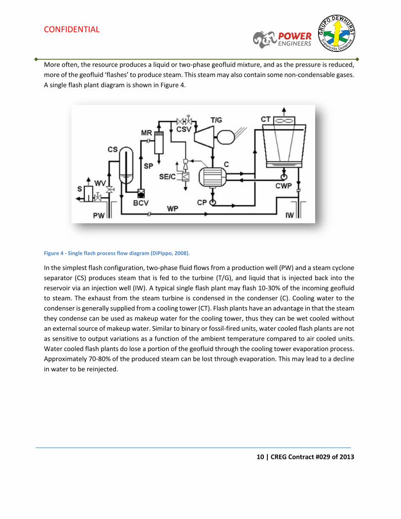
More often, the resource produces a liquid or two-phase geofluid mixture, and as the pressure is reduced,
more of the geofluid ‘flashes’ to produce steam. This steam may also contain some non-condensable gases.
A single flash plant diagram is shown in Figure 4.
Figure 4 - Single flash process flow diagram (DiPippo, 2008).
In the simplest flash configuration, two-phase fluid flows from a production well (PW) and a steam cyclone
separator (CS) produces steam that is fed to the turbine (T/G), and liquid that is injected back into the
reservoir via an injection well (IW). A typical single flash plant may flash 10-30% of the incoming geofluid
to steam. The exhaust from the steam turbine is condensed in the condenser (C). Cooling water to the
condenser is generally supplied from a cooling tower (CT). Flash plants have an advantage in that the steam
they condense can be used as makeup water for the cooling tower, thus they can be wet cooled without
an external source of makeup water. Similar to binary or fossil-fired units, water cooled flash plants are not
as sensitive to output variations as a function of the ambient temperature compared to air cooled units.
Water cooled flash plants do lose a portion of the geofluid through the cooling tower evaporation process.
Approximately 70-80% of the produced steam can be lost through evaporation. This may lead to a decline
in water to be reinjected.

CONFIDENTIAL
11 | CREG Contract #029 of 2013
Phases of a Geothermal Project
Regardless of the technology employed for a geothermal project, the execution phases and decision points
are similar. Table 1 describes these steps. In the initial phases of a project, little is known about the
reservoir. The identification phases attempt to define the extent and quality of the reservoir, and may use
exploration methods such as (DiPippo, 2008):
1. Literature surveys
2. Airborne surveys
3. Geologica studies
4. Hydrologic studies
5. Geochemical surveys
6. Geophysical surveys
If the reservoir appears promising, exploratory drilling is typically carried out, which attempts to better
characterize the nature of the geofluid and the potential productivity of wells. The methodology presented
in this study for the determination of energy output from a plant can be used to estimate output using a
small number of major independent variables that may be estimated at this stage: anticipated geofluid
temperature, flowrate, and ambient conditions. An average temperature is assumed for this methodology,
characteristic of an average produced temperature (or equivalent enthalpy) of all production wells for the
plant. Production well flowrates (kg/s) may be estimated from similar projects, or resource consultant
experience, but in truth flowrates cannot be known until the wells have been drilled and tested. Another
perspective would be to say the total flowrate required for a plant of a certain capacity can be known
precisely (if within reasonable limits for the reservoir’s capacity); what is unknown is the number of wells
that must be drilled in order to achieve that flowrate. The uncertainty of the output predictions would be
larger at this stage since the resource conditions and plant configuration is not yet finalized; this uncertainty
in output might be around 20-30%. As more wells are drilled and confidence in the characterization of the
reservoir improves, the output predictions would be refined.

CONFIDENTIAL
12 | CREG Contract #029 of 2013
Table 1 – Phases and decision points for typical geothermal projects (Deloitte, 2008)
If the exploratory drilling is promising, a decision must be made on more extensive production well drilling.
Drilling usually must be funded with equity and is not without risk. Typically feasibility studies would be
carried out at this stage to determine if, with the anticipated investment in wells and plant equipment, a
specific power plant design can deliver an acceptable return to the investors. At this stage more detailed
measurements of actual geofluid composition, enthalpy, and flow must be available. Feasibility studies
typically consider several cycle types, perform an economic optimization, and assess output using a model
that considers many more variables, including actual equipment performance estimates from vendor
quotes, flash pressures optimized considering the actual well production curves, and limitations on
reinjection temperature based on resource chemistry. As an example, for a prefeasibility study for a project
in Turkey, we provided various output estimates for different plant types that varied by less than 10%.
However, capital costs often have a greater impact on plant selection, and these varied by around 25%. It
is difficult to determine plant costs to an accuracy of better than 20-30% without doing a significant amount

CONFIDENTIAL
13 | CREG Contract #029 of 2013
of design and obtaining at least major equipment quotations. Obtaining output estimates in this stage of
the project is a process that may take weeks or months.
During this exploration and confirmation phases, numerical reservoir simulations are generally developed,
incorporating predictions for changes in temperature, pressure, or flowrates over time, and wellbore
losses. The model is updated as more data are available, with the most valuable being actual production
well long term flow testing and enthalpy measurements, among others.
Long term flow tests (weeks or months) may be preferred to better characterize wells, but permitting,
water disposal, or other limitations may mean only short term tests (hours or days) are possible in the
initial stages of the power plant definition. It often is preferred to carry out flow tests several months after
drilling is complete, to allow the well to heat back up if it has cooled from the drilling operations.
Measurement of single phase, low temperature flows are fairly straightforward, but flow and enthalpy
measurements for more energetic resources often require flashing the produced geofluid in a separator
and separately measuring the steam and water flows; this requires more significant investment in surface
equipment, and the emissions of steam and non-condensable gases during the test. With updated data
from long term tests, and using this reservoir model, the plant performance may be estimated over many
years of future production.
If the results of the feasibility study and confirmation drilling are promising, then a decision can be made
to proceed with the full construction of the project. The detailed design of a geothermal power plant and
the calculations to determine the guaranteed net output, that might serve for a contractual target and
regulatory acceptance, requires many months of effort, and relies on hundreds of items of data, many of
which are only available after purchase orders for major equipment are placed and much of the detailed
design is complete. These include values such as final design of the gathering and injection system, certified
motor data sheets, lighting loads, HVAC loads, miscellaneous pump operating times, and many other
factors. Obtaining output estimates in this stage of the project is a process that takes several years, and
these often include margins, depending on the commercial penalties that may apply for not meeting
performance.
After the plant is constructed and operated, variations in resource temperature, ambient conditions, and
the fact that design margins (excess heat exchanger areas for future fouling, excess pump capacity to
account for future wear, etc) may be present in equipment, result in the actual output inevitably varying
from the design point. It is not uncommon in our experience for the actual plant to perhaps outperform
the design performance by some 1-2%, or, if there are problems with the resource, output can be
significantly less than design.
The plant performance at the beginning of commercial operations is generally validated with a
performance test, the procedure for which is developed considering off-design performance curves in case

CONFIDENTIAL
14 | CREG Contract #029 of 2013
resource conditions, reservoir conditions, etc during the test period are different than the design values.
Tracking of capacity factor (or availability) over time is also generally done by the plant operator after
commercial acceptance, and may be an important issue related to warranties with the equipment or plant
suppliers.
Over the life of the plant, the resource may change as fluid is extracted, and output may decline. The
reservoir model can be updated for operating plants using actual flow and temperature (or enthalpy) data
from the wells, collected continuously or periodically. Generally, declines in well production are managed
by drilling additional makeup wells. Changes in geofluid chemistry or enthalpy sometimes make
modifications to plant equipment desirable after many years of operation.
In summary, the major objective of this study is to present a methodology to estimate the firm energy
output of a power plant, based on a manageable set of data that likely should be available to developers
or agencies at the initial stages of a project. We anticipate that in later phases, different and far more
detailed calculations, and performance tests during actual plant operation, would refine these output
estimates and gradually narrow the uncertainty bands.
Methodology
Design Point Output The first step in assessing the achievable annual energy output of a geothermal plant is to characterize the
nature of the fuel source, or in this case, the reservoir temperature (enthalpy), geofluid chemistry, and
flows. From that, we will proceed to examinations of how the different types of plants can convert this
geofluid to energy output. Initially, we will consider the design point output at annual average conditions,
and then progress to consider how this output may vary over the course of the year in order to determine
the annual energy output (Off-design point operation). We will progress in this evaluation from the lower
temperature resources (90 to 170 oC), where binary plants are more often used, to higher temperature
resources (140 to 300 oC), where flash plants are more often used.
Resource and Environmental Design Criteria
Since this is a general methodology intended to apply to a wide range of resources, we will express net
plant output and energy production in specific terms, i.e. kW or MWh per kg/s of total geofluid flow from
the production wells. In this way, the results will be scalable to projects of different sizes. We assume in
doing this that plant efficiency is not a strong function of plant size, which is a reasonable assumption.
The resource temperature (or produced geofluid enthalpy) will also vary between projects, so a range of
estimates across the aforementioned temperature bands are provided. Increasing resource temperature
helps boost plant output in two ways: the extractable energy is greater at higher temperatures, and the

CONFIDENTIAL
15 | CREG Contract #029 of 2013
efficiency with which heat energy can be converted to electrical power is also higher. Thus net plant specific
output is a strong function of resource temperature.
The ambient temperatures around the plant affect the size, cost, and performance of the cooling systems,
and influence net output. We provide output estimates for a range of dry (for air-cooled units) and wet
bulb (for water-cooled units) temperatures. Understand that simply by investing in larger and larger ACCs
and cooling towers, one can increase output, but our models assume that the designers would choose a
reasonable compromise between initial capital cost and plant output. We will present air-cooled binary
output curves for dry bulb temperatures in the range of 15 to 25 °C, and flash plant output curves for wet
bulb temperatures in the range of 10 to 20 °C.
Given that ambient temperature is an important factor in the plant design and performance, it is advisable
that developers begin harvesting this data early in the process. Since the reservoir exploration and drilling
is a process that may take many years, in parallel installing a weather station at the site, or verifying that
there is a reliable source of historical data nearby (existing weather stations within several kilometers,
perhaps) is advisable during this period. This is a low cost effort, but often overlooked, and a long data
interval is preferred to make informed decisions. Ideally dry bulb, wet bulb (or relative humidity), and wind
direction should be monitored.
The chemistry of the geofluid influences the lower temperature range of the geofluid that is to be injected.
This is more of a limitation for binary units, rather than the single flash units under consideration, since the
single flash separator operates at a relatively high temperature. We will use a constant injection
temperature limit of 75 oC for the binary units; actual conditions may differ at an individual site with more
or less dissolved solids. The flash process does lead to concentration of scaling materials; therefore the
injection temperature at each plant site needs to be evaluated on a case by case basis.
The ambient temperature and the operating conditions of the condenser also affect the minimum injection
temperature, as it is not possible to cool the brine further than below the temperature of the condensed
working fluid, even if in theory the limit on precipitation of solids is lower. Operation of binary units at very
low resource temperatures (<100 oC) thus may only be economic in colder climates, where the injection
temperature can be lowered such that more energy can be extracted; this was the case at plants such as
Husavik in Iceland and Chena Hot Springs in Alaska.
Lower Temperature Resources – Binary Plant Evaluation
To evaluate plant output at the design point conditions, we constructed a model using typical equipment
sizing parameters, equipment efficiencies, and configurations for the binary cycle. These parameters
include:
Heat exchanger minimum temperature differences between the hot and cold fluid streams,

CONFIDENTIAL
16 | CREG Contract #029 of 2013
Pressure drops in piping and equipment,
Turbine, gearbox, and generator efficiencies,
Heat exchanger temperature differences, and
Pump efficiencies.
While it is possible to adjust these parameters to get more or less output to some degree, we have chosen
reasonable industry standards that will result in a plant of both reasonable efficiency and capital cost.
Since different binary package suppliers use different working fluids, we compiled estimated net specific
power outputs across the given temperature ranges for three commonly used working fluids: isobutane,
isopentane, and the refrigerant R-245fa. Our performance estimating tool is constructed in Excel and relies
on fluid property database functions from REFPROP. This software is provided by the U.S. National Institute
of Standards (NIST) and provides reliable property data for a wide range of substances, including water.
In order to simplify the analysis, certain parameters were set so that the only variables we input were the
brine inlet temperature and the air inlet temperature. Figure 5 shows a sample of the binary model output
operating at 120 °C geofluid inlet temperature and 20 °C dry bulb temperature. For this case the working
fluid is isobutane. Gross power output is 9,043 kW and total plant parasitic power to drive various pumps
and fans is 2,173 kW.
Note that this power consumption value does not include any gathering system loads, such as production
or injection well pumps; since the nature of the resource is not known, these cannot be determined at this
time in this study. The variation in production or injection well pump loads is so great that it would be
unrealistic to include them in the formulas in this study. Some production wells are artesian, flowing
without requiring pumping. Some may require production well pumps, with power consumption of up to
around 0.5 MW per production well. Without knowing the specific characteristics of the resource and the
wells drilled, it would cloud the analysis to include it in the base case estimates.
Similarly for injection wells, there can be great variations in the injection pressure, and pumping power,
required. Some injection wells operate under a vacuum, with no pumping power required. Some operate
at pressures that may be as high as 50-60 bar. The injection pumps might consume somewhere between
0-5% of net power, thus including an allowance would cloud the analysis. Developers should consider
modifying the net output estimates included in this study to incorporate production or injection pumps,
once they have better information from their resource consultants.

CONFIDENTIAL
17 | CREG Contract #029 of 2013
Figure 5 - Typical binary (air-cooled) model screenshot.
The geofluid releases energy in the vaporizer and preheater; with the minimum temperature approach
adjusted to a reasonable value to give a balance between efficiency and economy. The vaporized working
fluid passes through a turbine and is condensed in the ACC. The feed pump returns the working fluid to
the preheater. The major parasitic loads are the feed pump, ACC fans, transformer losses, and an
allowance for miscellaneous other loads.
The net power is divided by the total geofluid flowrate to obtain a net plant specific power output of 12.4
kW/ (kg/s) at the design point for the conditions of Figure 5. The net plant specific power consumption is
plotted as a function of resource temperature.

CONFIDENTIAL
18 | CREG Contract #029 of 2013
Variations in working fluid
As stated earlier, for different resources different working fluids may be able to generate different
outputs. Thus, we generated curves for isobutane, isopentane, and R-245fa. The comparison of results
can be seen in Figure 6.
Figure 6 - Net air-cooled binary plant specific output as a function of resource temperature at 15 °C dry bulb temperature.
The working fluid that generates the highest net plant specific power is not necessarily the preferred
option, as the economics of cycles based on different working fluids may also vary. There may also be non-
economic considerations such as the desire by the owner to standardize on a certain working fluid for
multiple plants, flammability concerns, or other factors. Overall the power generation by the different
working fluids can be seen to be comparable across most of the temperature ranges. Therefore, the figures
in this report are based on an average specific net power output for the three working fluids isobutane,
isopentane and R245fa.
Figure 7 shows the variation of power for a binary cycle using an average of the three working fluids over
a range of geofluid temperatures. It can be seen that there is a strong correlation between geofluid
temperature and output; as the temperature rises, both the quantity of extractable energy increases, and
also the conversion efficiency from thermal to electrical power.
0
5
10
15
20
25
30
35
40
45
50
80 100 120 140 160 180
Sp
ecif
ic N
et P
ow
er [
kW
/(k
g/s
)]
Resource Temperature (degC)
Isobutane
Isopentane
R245fa

CONFIDENTIAL
19 | CREG Contract #029 of 2013
Figure 7 - Net air-cooled binary plant specific output as a function of resource temperature at 15 °C DBT.
Variations in ambient temperature
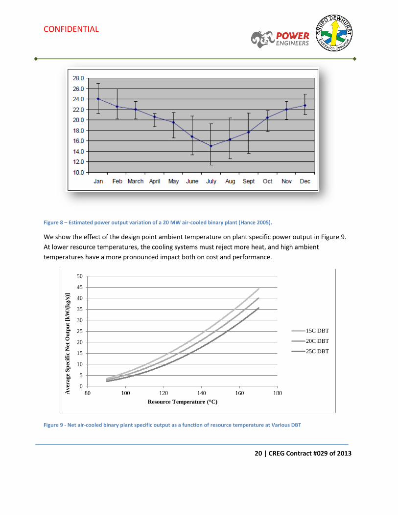
Ambient temperature has a profound impact on the performance and economics of the plant. Hance
(2005) provided a curve of average output of a nominal 20 MW binary air-cooled plant as it varies month
to month, shown in Figure 8. In a tropical location where annual average temperatures are high, the plant
cost per installed kW is higher and net power output lower, than if it were in a colder location.
0
5
10
15
20
25
30
35
40
45
50
80 90 100 110 120 130 140 150 160 170 180
Aver
age
Sp
ecif
ic N
et O
utp
ut
[kW
/(k
g/s
)]
Resource Temperature (°C)
CONFIDENTIAL
20 | CREG Contract #029 of 2013
Figure 8 – Estimated power output variation of a 20 MW air-cooled binary plant (Hance 2005).
We show the effect of the design point ambient temperature on plant specific power output in Figure 9.
At lower resource temperatures, the cooling systems must reject more heat, and high ambient
temperatures have a more pronounced impact both on cost and performance.
Figure 9 - Net air-cooled binary plant specific output as a function of resource temperature at Various DBT
0
5
10
15
20
25
30
35
40
45
50
80 100 120 140 160 180Aver
ag
e S
pec
ific
Net
Ou
tpu
t [k
W/(
kg
/s)]
Resource Temperature (°C)
15C DBT
20C DBT
25C DBT

CONFIDENTIAL
21 | CREG Contract #029 of 2013
Design point power predictions
We combine the results of the explorations of resource temperature, working fluid, and ambient
temperature to develop an overall curve of net plant specific output. An equation is proposed to fit these
points for an average of the three working fluids (isobutane, isopentane and R245fa):
𝒛 = (𝟑. 𝟑𝟖𝟐 𝒙 𝟏𝟎−𝟑)𝒙𝟐 − (𝟐. 𝟒𝟖𝟏 𝒙 𝟏𝟎−𝟑)𝒚𝟐 − (𝟗. 𝟑𝟒𝟗 𝒙 𝟏𝟎−𝟑)𝒙𝒚 − 𝟎. 𝟐𝟐𝟗𝒙 + 𝟎. 𝟖𝟎𝟎𝒚 − 𝟐. 𝟏𝟔𝟕 (Eqn 1)
Where 𝑧 is the specific net output [kW/ (kg/s)], 𝑥 is the resource temperature (°C) and 𝑦 is the dry bulb
temperature (°C).
The model output can be compared to historical data from operating plants. Table 2 shows data from
selected binary plants around the world in order to check the agreement between model output and actual
plant data, where available in the public domain.
Table 2 – Historical plant data, adapted from DiPippo (2004).
Plant
Approximate Reservoir
Temperature
(oC)
Assumed Design
Dry Bulb
Temperature
(oC)
Actual Plant Net Plant
Specific Output
(kW/(kg/s)
Brady 107.8 16.8 8.9
Nigorikawa 140 13 20
Stillwater 155 13 37
Heber SIGC 165 15 54.5
Binary Plant 1 135 14 22.4
Binary Plant 2 96 2 8.1
Binary Plant 3 157 74 40.2
As stated, the complexity of the cycle, investments in cycle equipment, and variations in injection
temperature can result in performance that is less or more than the model predictions. Figure 10 shows
the actual plant performance overlaid with predicted performance of binary plants at a constant 15 oC dry
bulb temperature, including some confidential and unnamed plants. Overall the agreement is fairly good,
but there can be deviations. The Heber SIGC plant, for example, is a dual pressure level cycle, which is more
complex but which offers some advantages over the single pressure cycle used in the binary model. As a
result, one might expect that actual plant performance may differ from the model predictions within a
band of some 10-20%.

CONFIDENTIAL
22 | CREG Contract #029 of 2013
Figure 10 - Comparison of binary plant model predictions and historical plant output.
Higher Temperature Resource – Flash Plant Evaluation
As resource temperatures and enthalpies rise, flash plants become an increasingly economical option over
binary plants, although they can be competitive with one another in an overlapping temperature range
around 150-190 oC. Bombarda and Macchi (2000) presented an economical and technical performance
comparison that covers these aspects in more detail. For the purposes of this study, we looked at resource
temperatures above 140 °C.
Single flash plants generate additional steam from the brine of the first flash and are the most common
flash configuration. However, double and triple flash plants exist, as well. A double flash plant might add
10% in output, but incur additional capital costs for the gathering system, separators, and turbine. The
lower temperature of the lower pressure flash can also lead to scaling concerns in the low pressure brine.
Since the resource chemistry is undefined, and since single flash is a common choice for developers, the
single flash cycle was chosen for the base case flash model.
As for the binary cycle, we constructed a model using typical equipment sizing parameters, equipment
efficiencies, and configurations for the flash cycle. These parameters, for which reasonable industry
standards have been applied, include:
Brady
Stillwater
Nigorikawa
Heber SIGC
Binary Plant 1
Binary Plant 2
Binary Plant 3
0
10
20
30
40
50
60
80 90 100 110 120 130 140 150 160 170 180
Aver
age
Sp
ecif
ic N
et O
utp
ut
[kW
/(k
g/s
)]
Resource Temperature (°C)

CONFIDENTIAL
23 | CREG Contract #029 of 2013
Separator (flash) pressure,
Pressure drops in piping and equipment,
Turbine and generator efficiencies,
Pump and fan efficiencies,
Condenser sub-cooling, and
Cooling tower range and approach.
The selection of the optimum separator pressure is relatively complex for a real project, as it depends on
the enthalpy of the resource, deliverability of the wells, and the scaling potential of the geofluid. For this
study, we use a principle described by DiPippo (2008), which is that the theoretical optimum single flash
temperature is midway between the resource temperature and the condenser temperature. For the
purposes of the separator temperature estimation, we assume a condenser temperature of 50 oC; this
value is an economic optimization that would be developed during detailed thermodynamic design. This
equal temperature split principle provides a reasonable point for power output estimation; if actual flash
pressures are slightly different, they do not affect the power output estimate markedly.
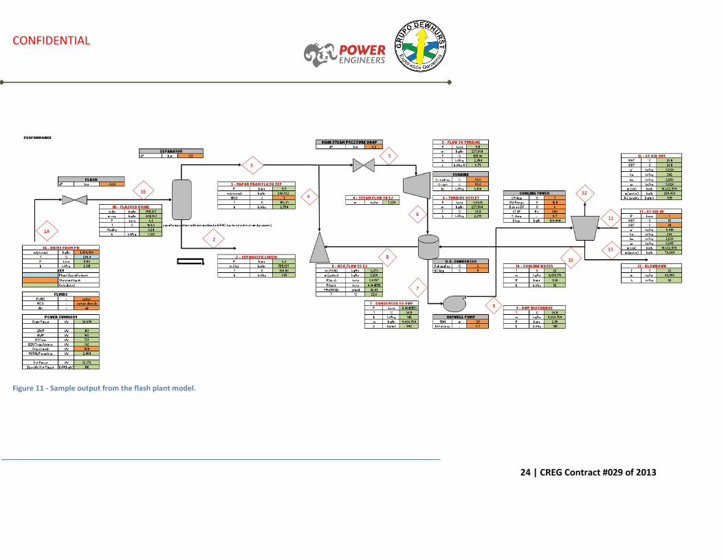
Figure 11 shows sample model output from a base case flash plant, operating at 270 °C geofluid inlet
temperature and 15 °C wet bulb temperature. Gross power output is 34,670 kW and total plant parasitic
power to drive various pumps and fans is 2,494 kW. Note that this power consumption value does not
include any gathering system loads, such as production or injection well pumps; since the nature of the
resource is not known, these cannot be determined at this time.
CONFIDENTIAL
24 | CREG Contract #029 of 2013
Figure 11 - Sample output from the flash plant model.

CONFIDENTIAL
25 | CREG Contract #029 of 2013
Geofluid from the resource enters the separator and is flashed at the separator pressure. A pressure drop
is assigned to the steam flowing from the separator to the turbine. The steam expands through the turbine
to the lower pressure of the condenser. The direct contact condenser is cooled by water from the cooling
tower, drawn into the condenser by its vacuum. The combination of condensed steam and cooling water
is pumped by hotwell pumps back to the cooling tower. Some non-condensable gases (NCG) which would
normally be present in geothermal steam must be removed from the condenser to maintain vacuum; these
are drawn out by the gas removal system. In this case, a hybrid two stage ejector/liquid ring vacuum pump
(LRVP) arrangement is proposed, which is a relatively efficient arrangement. The major consumers of
parasitic power in the plant are the hotwell pumps, cooling tower fans, LRVP, and main transformer losses.
An allowance has been added for other minor loads such as HVAC, lighting, miscellaneous pumps, etc.
The total parasitic loads are subtracted from the gross steam turbine generator output to find the net
power, and this is divided by the total inlet geofluid flow to determine the net plant specific power. In the
example shown above, the specific net power is 116 kW/ (kg/s of total geofluid flow into the flash plant).
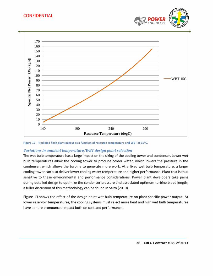
Figure 12 shows flash plant power variation as a function of geofluid equivalent resource temperature.
CONFIDENTIAL
26 | CREG Contract #029 of 2013
Figure 12 - Predicted flash plant output as a function of resource temperature and WBT at 15°C.
Variations in ambient temperature/WBT design point selection
The wet bulb temperature has a large impact on the sizing of the cooling tower and condenser. Lower wet
bulb temperatures allow the cooling tower to produce colder water, which lowers the pressure in the
condenser, which allows the turbine to generate more work. At a fixed wet bulb temperature, a larger
cooling tower can also deliver lower cooling water temperature and higher performance. Plant cost is thus
sensitive to these environmental and performance considerations. Power plant developers take pains
during detailed design to optimize the condenser pressure and associated optimum turbine blade length;
a fuller discussion of this methodology can be found in Saito (2010).
Figure 13 shows the effect of the design point wet bulb temperature on plant specific power output. At
lower reservoir temperatures, the cooling systems must reject more heat and high wet bulb temperatures
have a more pronounced impact both on cost and performance.
0
10
20
30
40
50
60
70
80
90
100
110
120
130
140
150
160
170
140 190 240 290
Sp
ecif
ic N
et P
ow
er [
kW
/(k
g/s
)]
Resource Temperature (degC)
WBT 15C

CONFIDENTIAL
27 | CREG Contract #029 of 2013
Figure 13 – Net flash plant specific output as a function of resource temperature and various WBT.
For the flash plant, the best fit curves to the data were third order. In order to simplify the equations, we
split the plots into three resource temperature ranges: 140-180 C, 180-240 C and 240-300 C. For each of
these temperature ranges, we developed models of operation at three different wet bulb temperatures. A
surface was mapped showing output as a function of both reservoir and wet bulb temperatures, and curves
fit to a two parameter equation:
140 to ≤ 180°C
𝒛 = (−𝟐. 𝟖𝟐𝟓 𝒙 𝟏𝟎−𝟑)𝒙𝟐 − (𝟖. 𝟓𝟐𝟒 𝒙 𝟏𝟎−𝟒)𝒚𝟐 − (𝟒. 𝟎𝟓𝟕 𝒙 𝟏𝟎−𝟑)𝒙𝒚 + 𝟏. 𝟕𝟏𝟔𝒙 + 𝟎. 𝟏𝟑𝟐𝒚 − 𝟏𝟕𝟒. 𝟒𝟐𝟗 (Eqn 2)
>180 to ≤ 240°C
𝒛 = (𝟐. 𝟏𝟑𝟐 𝒙 𝟏𝟎−𝟑)𝒙𝟐 − (𝟐. 𝟏𝟒𝟔 𝒙 𝟏𝟎−𝟒)𝒚𝟐 − (𝟓. 𝟎𝟖𝟗 𝒙 𝟏𝟎−𝟑)𝒙𝒚 + (𝟏. 𝟏𝟎𝟗 𝒙 𝟏𝟎−𝟐)𝒙 + 𝟎. 𝟐𝟗𝟓𝒚 −𝟐𝟕. 𝟖𝟑𝟓 (Eqn 3)
> 240 to 300°C
𝒛 = (𝟐. 𝟓𝟑𝟎 𝒙 𝟏𝟎−𝟑)𝒙𝟐 + (𝟑. 𝟐𝟔𝟐 𝒙 𝟏𝟎−𝟑)𝒚𝟐 − (𝟔. 𝟒𝟗𝟖 𝒙 𝟏𝟎−𝟑)𝒙𝒚 − (𝟖. 𝟑𝟗𝟔 𝒙 𝟏𝟎−𝟐)𝒙 + 𝟎. 𝟓𝟑𝟐𝒚 − 𝟐𝟕. 𝟖𝟐𝟐 (Eqn 4)
0
10
20
30
40
50
60
70
80
90
100
110
120
130
140
150
160
170
140 190 240 290
Sp
ecif
ic N
et P
ow
er [
kW
/(k
g/s
)]
Resource Temperature (degC)
WBT 10C
WBT 15C
WBT 20C

CONFIDENTIAL
28 | CREG Contract #029 of 2013
Where 𝑧 is the specific net output [kW/(kg/s)], 𝑥 is the resource temperature (°C) and 𝑦 is the dry bulb
temperature (°C).
Design point power predictions
The equation output can be compared to historical data from operating plants. Table 3 illustrates the
agreement between model output and actual plant data, where available in the public domain.
Table 3 – Comparison of model predictions and historical plant output for flash plants.
Plant
Approximate
Reservoir
Temperature
(oC)
Assumed
Design Wet
Bulb
Temperature
(oC)
Actual Plant
Net Plant
Specific Output
(kW/(kg/s)
Predicted Net
Plant Specific
Output
(kW/(kg/s))
Deviation
(%)
Kizildere I 200 12 39.5 51 29.1%
Miravalles III 241 22.8 77 86 11.7%
Olkaria II 270 12 111 119 7.2%
Cerro Prieto IV 320 17 174 184 5.7%
San Jacinto 260 25 117 94 19.7%
It can be seen that the general trend is towards higher specific output at the higher resource temperatures.
The model may vary from actual plant performance due to more or less investment in cooling systems
which increase efficiency, non-condensable gas content in the reservoir, or other factors. Kizildere I was an
older plant that operates with very high non-condensable gas content (>20% of total steam flow); thus the
model predicts significantly higher performance than actual. For more modern plants with more normal
resource conditions, the model appears to be able to predict plant output to within 10%.
Figure 14 shows the actual plant performance overlaid with predicted performance of flash plants. Overall
the agreement is fairly good, but there can be deviations. The performance of several unnamed (due to
confidentiality) plants are shown, in addition to those from Table 3.

CONFIDENTIAL
29 | CREG Contract #029 of 2013
Figure 14 - Comparison of flash plant model predictions and historical plant output.
Off-Design Operation The previous sections presented the development of a model that would predict instantaneous plant
output at the design point. This output may vary over the course of a day or year. The capacity factor is
defined as the actual energy output of the plant during a time period, divided by the energy output it would
be capable of if it ran at the design point power. Capacity factors for other renewable sources such as wind
or solar are typically less than 40%, however since geothermal plants are provided with a virtually
uninterruptible fuel source, capacity factors may be well above 90%.
Two factors serve to reduce capacity factor, and we will discuss each of these in the next sections:
temperature variations and outages. This analysis does not consider any impact of production well declines
on output, which may typically be 1-4% per year; it is assumed that makeup well drilling is sufficient to
offset these declines.
Annual temperature variations and impact
It was discussed earlier that colder temperatures allow for better cooling of the various cycles and increase
design power output. After the plant is built, power output also varies as the plant experiences variations,
both diurnally and seasonally. A typical plant will have a correction curve that captures the impact on net
Kizildere I
Miravalles III
Olkaria II
Cerro Prieto IV
San Jacinto
Flash Plant 1
Flash Plant 2
Flash Plant 3
130 150 170 190 210 230 250 270 290 310 330 350
Sp
ecif
ic N
et P
ow
er [
kW
/(k
g/s
)]
Resource Temperature (degC)
WBT 10C
WBT 15C
WBT 20C
CONFIDENTIAL
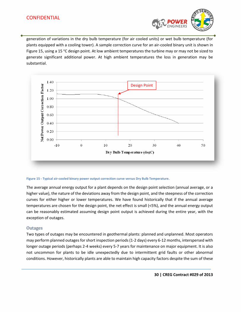
30 | CREG Contract #029 of 2013
generation of variations in the dry bulb temperature (for air cooled units) or wet bulb temperature (for
plants equipped with a cooling tower). A sample correction curve for an air-cooled binary unit is shown in
Figure 15, using a 15 oC design point. At low ambient temperatures the turbine may or may not be sized to
generate significant additional power. At high ambient temperatures the loss in generation may be
substantial.
Figure 15 - Typical air-cooled binary power output correction curve versus Dry Bulb Temperature.
The average annual energy output for a plant depends on the design point selection (annual average, or a
higher value), the nature of the deviations away from the design point, and the steepness of the correction
curves for either higher or lower temperatures. We have found historically that if the annual average
temperatures are chosen for the design point, the net effect is small (<5%), and the annual energy output
can be reasonably estimated assuming design point output is achieved during the entire year, with the
exception of outages.
Outages
Two types of outages may be encountered in geothermal plants: planned and unplanned. Most operators
may perform planned outages for short inspection periods (1-2 days) every 6-12 months, interspersed with
longer outage periods (perhaps 2-4 weeks) every 5-7 years for maintenance on major equipment. It is also
not uncommon for plants to be idle unexpectedly due to intermittent grid faults or other abnormal
conditions. However, historically plants are able to maintain high capacity factors despite the sum of these
Design Point

CONFIDENTIAL
31 | CREG Contract #029 of 2013
two effects. To some degree the outage periods are a function of the owner’s investments in the operations
and maintenance budgets. Table 3 shows typical capacity factors from plants around the world that reflect
these combined influences of environment and outages.
Table 3 – Capacity factors by selected countries (adapted from Lund et al, 2010).
Country Number of
Units
Running Capacity
Factor
United States 209 94%
Indonesia 22 92%
Iceland 25 91%
Kenya 10 98%
Typically, about 0.8% degradation in plant output per year occurs in between major equipment
maintenance. About 80% of the degradation loss will be recovered during the year of the outage. The
degradation loss is usually incorporated into the running capacity factor. For the purposes of this study, we
will assume a constant capacity factor of 95% will apply; thus the annual firm energy output from the plant
can be calculated as:
𝑴𝑾𝒉 =
𝑫𝒆𝒔𝒊𝒈𝒏 𝑷𝒐𝒊𝒏𝒕 𝑵𝒆𝒕 𝑷𝒍𝒂𝒏𝒕 𝑺𝒑𝒆𝒄𝒊𝒇𝒊𝒄 𝑷𝒐𝒘𝒆𝒓 [𝒌𝑾𝒌𝒈𝒔
] 𝒙 𝑮𝒆𝒐𝒇𝒍𝒖𝒊𝒅 𝒇𝒍𝒐𝒘 (𝒌𝒈
𝒔)𝒙 𝟎.𝟗𝟓 𝒙 𝟖,𝟕𝟔𝟔
𝒉𝒐𝒖𝒓𝒔
𝒚𝒆𝒂𝒓
𝟏𝟎𝟎𝟎𝒌𝑾𝒉
𝑴𝑾𝒉
(Eqn 5)
Table 4 shows sample calculations of annual energy output for two types of resource; a lower temperature
setting where a binary plant may be more economical, and a higher temperature plant for which flash
might be more economical. The equations presented are used to calculate both the specific power output
and the annual firm energy prediction, using assumed values for the independent variables.

CONFIDENTIAL
32 | CREG Contract #029 of 2013
Table 4 – Sample calculations of firm energy output for two resources
Parameter Units Resource #1 Resource #2
Reservoir temperature oC 150 250
Cycle type assumed - Binary, air cooled
Flash, water cooled
Ambient temperature oC 20
(dry bulb) 15
(wet bulb)
Design point specific power output kW/(kg/s) 26.6 93.64
Geofluid flow kg/s 500 1000
Plant design point output MW 27.1 93.64
Annual firm energy output MWh 110,656 779,828
Discussion
Output Uncertainty Depending on the equipment supplier, cycle complexity, technology, and commercial factors, actual plants
may have output more or less than these values. There are hundreds of parameters that affect the total
annual output of a geothermal plant, including many economic optimization parameters. For example, the
size of heat exchangers, the choice between an inexpensive but less efficient pump, the efficiency of
different vendor’s turbines, non-condensible gas content in the geofluid, injection pressures, and many
other characteristics. These may even change over the life of the project as the resource evolves. Since
very few input parameters are generally available at an initial assessment of a project, we chose those that
have the greatest impact on the annual energy output, and assume reasonable values for others. Due to
these factors, and in comparing the predictions with historical data, we feel that an uncertainty of +10% in
annual energy output would be a reasonable assessment to account for these variations.
Correlations Equations 1-4 were plotted to one graph (Figure 16) to show the correlation between the binary and flash
models. For the binary equation (Eqn 1), a dry bulb temperature of 20°C was used. For the flash equations
(Eqns 2-4), a wet bulb temperature of 15°C was used.

CONFIDENTIAL
33 | CREG Contract #029 of 2013
Figure 16 – Plot of flash and binary equations
The annual net energy prediction per kg/s would be incorporated into equation 5 to obtain a firm energy
prediction in MWh of net plant output for a year.
It has been discussed that economic parameters may lead to the selection of a different cycle than what
Figure 16 might estimate is preferred for the resource temperature. It is not uncommon for air-cooled
binary plants to be used, for example, at locations where water cooling, evaporation, and net loss of fluid
from the reservoir cannot be tolerated, even though the resource temperatures are high. Small modular
binary units (<5 MW) may also be more appealing below a certain project size, due to their more modular
nature than flash plants, even if the resource temperature is higher.
Monte Carlo Analysis A Monte Carlo statistical analysis could be performed using these models to assess the uncertainty in
annual energy output as a function of uncertainties in reservoir characteristics (flow,
enthalpy/temperature, non-condensable gas content, e.g.), ambient temperatures, capacity factor, and
other variables as desired.
0
20
40
60
80
100
120
140
160
180
90 110 130 150 170 190 210 230 250 270 290 310
Sp
ecif
ic N
et P
ow
er [
kW
/(k
g/s
)]
Resource Temperature (degC)
Flash 140 to 180C
Flash 180 to 240C
Flash 240 to 300C
Binary 90 to 170C

CONFIDENTIAL
34 | CREG Contract #029 of 2013
Each component of the equations has inherent uncertainty as to what the true value will be. For instance,
wells may underperform in terms of flow, assumed brine temperatures may not be representative for the
long term resource, and the performance of key equipment may vary from assumed values after detailed
design has finished. Each potential deviation from the assumed values of the input parameters contributes
to uncertainty in the output parameters. A Monte Carlo simulation is one method of quantifying the
cumulative effect of these uncertainties and reporting their impact on the uncertainty in overall plant
metrics such as Specific Power or Net Plant Output.
The Monte Carlo simulation requires that the uncertainty in the input parameters be represented in the
form of probability density functions (also called probability distributions). Triangular distributions as
shown in Figure 17 are often employed for this purpose because they are easy to create, have clearly
defined minimum and maximum boundaries, and allow skewed distributions to be utilized without
significant complexity. This is in contrast to the more familiar bell shaped distributions. Triangular probably
density functions are also computationally simple and allow higher numbers of simulations to be run in the
same amount of computer processing time.
Figure 17 – Typical triangular distribution used to simulate a normal distribution (Denker, 2013)
Different parameters would have different uncertainties, and hence ‘width’ of the triangular distribution
function, depending on the phase of the project. For example, annual average temperature might be
known quite well at a specific location with weather station data spanning many years; the uncertainty
might be +/-1 oC. However, the triangular distribution of resource temperature might be +/-5 oC, depending
on the stage of exploration.
The Monte Carlo simulation method uses pseudo random numbers generated by a computer to pick values
for the input parameters based on their probability density functions. The selected values represent a
statistically realistic guess for each of the input parameters to be used in the calculation of plant metrics.
The Monte Carlo simulation solves the plant model and estimates the key plant parameters based upon
the guesses and stores these values for subsequent analysis. This is repeated many times, with simulation
counts ranging from tens of thousands to tens of millions.

CONFIDENTIAL
35 | CREG Contract #029 of 2013
The number of simulations required for a Monte Carlo calculation depends on the desired accuracy and
the variance in the input parameters, but 10,000 is often considered to be a minimum number to achieve
reasonable accuracy. A high number of simulations will assure that the results reflect primarily uncertainty
in the input parameters rather than uncertainty in the Monte Carlo simulation itself. When the number of
simulations is sufficiently high, multiple Monte Carlo analyses using the same number of simulations will
yield consistent results for uncertainty. Garg (2010) provides a more detailed illustration of this
methodology, which can produce an estimate of probable reservoir potential, as shown in Figure 18. Figure
18 shows that for this sample reservoir, there may be a 90% probability of it having 40 MW of potential
production, and a 50% probability of 80 MW.
Figure 188 – Cumulative probability distribution curve of reservoir potential for a sample project (Garg, 2010)
The probability distribution functions for the input parameters used in the present study have not been
defined and thus no Monte Carlo simulation has been performed on either a specific reservoir or plant
output. However, future efforts to enhance a plant performance estimate may benefit from using Monte
Carlo simulation to quantify the uncertainty in Specific Power and Plant Net Output. Such an improvement
would allow an upper and lower bound with a particular confidence level to be provided with the calculated
values of the plant metrics.
An example of the sensitivity of binary plant output to changes in the input parameters can be seen in Table
5. The working fluid used in this example is isobutane. Using a typical 150 oC resource as shown in Table 4,
we vary one parameter at a time and report the variations in output (MW). Output is directly proportional
to geofluid flow, somewhat sensitive to reservoir temperature, and less sensitive to ambient temperature.

CONFIDENTIAL
36 | CREG Contract #029 of 2013
Table 5 – Sample calculation showing effect of variation in parameters on output
Parameter Units
Original
Basis
Modified
Geofluid Flow
Modified brine inlet
temperature
Modified ambient
temperature
Geofluid flow kg/s 500 550 500 500
Brine inlet
temperature oC 150 150 151 150
Ambient
temperature oC
20 (dry bulb)
20 20 19
Resultant Output MW 15.51 17.08 15.82 15.76
Since the probability distribution functions for the current analyses are not well defined, this uncertainty
analysis was not performed; however Monte Carlo analysis to develop a range of probable plant outputs
would be a path for future research or effort by developers on a specific project, one for which the resource
conditions and attendant uncertainties are better known.
Conclusion This report has provided correlations for the reasonable estimation of annual firm energy output from a
geothermal plant, given as inputs a small set of assumptions such as total geofluid flow, resource
temperature, and ambient temperature. Variations in technology or optimization for a specific site may
result in output different from this estimation, however based on historical data it appears the uncertainty
is within 10% for the majority of projects. The report provides background on the sensitivity of plant energy
output as a function of many variables.
The estimation of annual firm energy output also assumes that there is sufficient reservoir capacity to
maintain the design geofluid flow and temperature. Details of specific reservoir conditions may require
added reduction in annual net output if there is a non-recoverable degradation in the reservoir geofluid
supply condition.

CONFIDENTIAL
37 | CREG Contract #029 of 2013
References
Bombarda P, Macchi E. 2000. Optimum cycles for geothermal power plants. Proceedings of the World
Geothermal Congress; 2000 May 28- June 10; Kyushu-Tohoku, Japan.
Deloitte, 2008. Geothermal Risk Mitigation Strategies Report. Prepared for the DOE Office of Energy
Efficiency and Renewable Energy Geothermal Program.
DiPippo R. 2008. Geothermal Power Plants: Principles, Applications, Case Studies and Environmental
Impact. Oxford (UK): Elsevier.
DiPippo, R. 2004. Second law assessment of binary plants generating power from low temperature
geothermal fluids. Geothermics 33:565-586.
Garg S. 2010. Appropriate use of USGS volumetric “heat in place” method and Monte Carlo calculations.
Proceedings, Thirty-Fourth Workshop on Geothermal Reservoir Engineering; 2010 Feb 1-3, Stanford,
California.
Hance C. 2005. Factors affecting costs of geothermal power development. Washington (DC): Geothermal
Energy Association.
Lund JW, Bertani R. 2010. Worldwide geothermal utilization 2010. GRC Transactions, Vol. 34.
NREL. 2010. Cost and performance assumptions for modeling electricity generation technologies. NREL,
Golden, CO: 2010. NREL/SR-6A20-48595.
Saito S. 2010. Technologies for higher performance and reliability of geothermal power plant.
Proceedings of the World Geothermal Congress; 2010 Apr 25-29; Bali, Indonesia.
Thorsteinsson H, Augustine C, Anderson BJ, Moore MC, Tester JW. 2008. The impacts of drilling and
reservoir technology advances on EGS exploitation. Proceedings, Thirty-Third Workshop on Geothermal
Reservoir Engineering; 2008 Jan 28-30, Stanford, California.