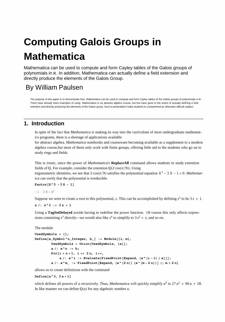
Computing Galois Groups in MathematicaMathematica can be used to compute and form Cayley tables of the Galois groups of polynomials in R. In addition, Mathematica can actually define a field extension and directly produce the elements of the Galois Group.

By William Paulsen

The purpose of this paper is to demonstrate how Mathematica can be used to compute and form Cayley tables of the Galois groups of polynomials in R.

There have already been examples of using Mathematica in an abstract algebra course, but few have gone to the extent of actually defining a field

extention and directly producing the elements of the Galois group. Such a presentation helps students to comprehend an otherwise difficult subject.

1. IntroductionIn spite of the fact that Mathematica is making its way into the curriculum of most undergraduate mathemat-ics programs, there is a shortage of applications availablefor abstract algebra. Mathematica notebooks and courseware becoming available as a supplement to a modernalgebra course,but most of them only work with finite groups, offering little aid to the students who go on tostudy rings and fields.

This is ironic, since the power of Mathematica's ReplaceAll command allows students to study extentionfields of Q. For example, consider the extention QH2 cosHΠ �9LL. Using trigonometric identities, we see that 2 cosHΠ �9L satisfies the polynomial equation X 3 - 3 X - 1 = 0. Mathemat-ica can verify that the polynomial is irreducible.

Factor@X^3 - 3 X - 1D

-1 - 3 X + X3

Suppose we were to create a root to this polynomial, z. This can be accomplished by defining z3 to be 3 z + 1.

z �: z^3 := 3 z + 1

Using a TagSetDelayed avoids having to redefine the power function. Of course this only affects expres-sions containing z3 directly---we would also like z4 to simplify to 3 z2 + z, and so on.

The module

UsedSymbols = 8<;

Define@a_Symbol^n_Integer, b_D := Module@8i, m<,

UsedSymbols = Union@UsedSymbols, 8a<D;

a �: a^n := b;

For@i = n + 1, i <= 2 n, i++,

a �: a^i := Evaluate@FixedPoint@Expand, Ha^Hi - 1L L aDDD;

a �: a^m_ := FixedPoint@Expand, Ha^H2 nLL Ha^Hm - 2 nLLD �; m > 2 nD

allows us to create definitions with the command

Define@a^3, 3 a + 1D

which defines all powers of a recursively. Thus, Mathematica will quickly simplify a9 to 27 a2 + 90 a + 28.In like manner we can define QHaL for any algebraic number a.

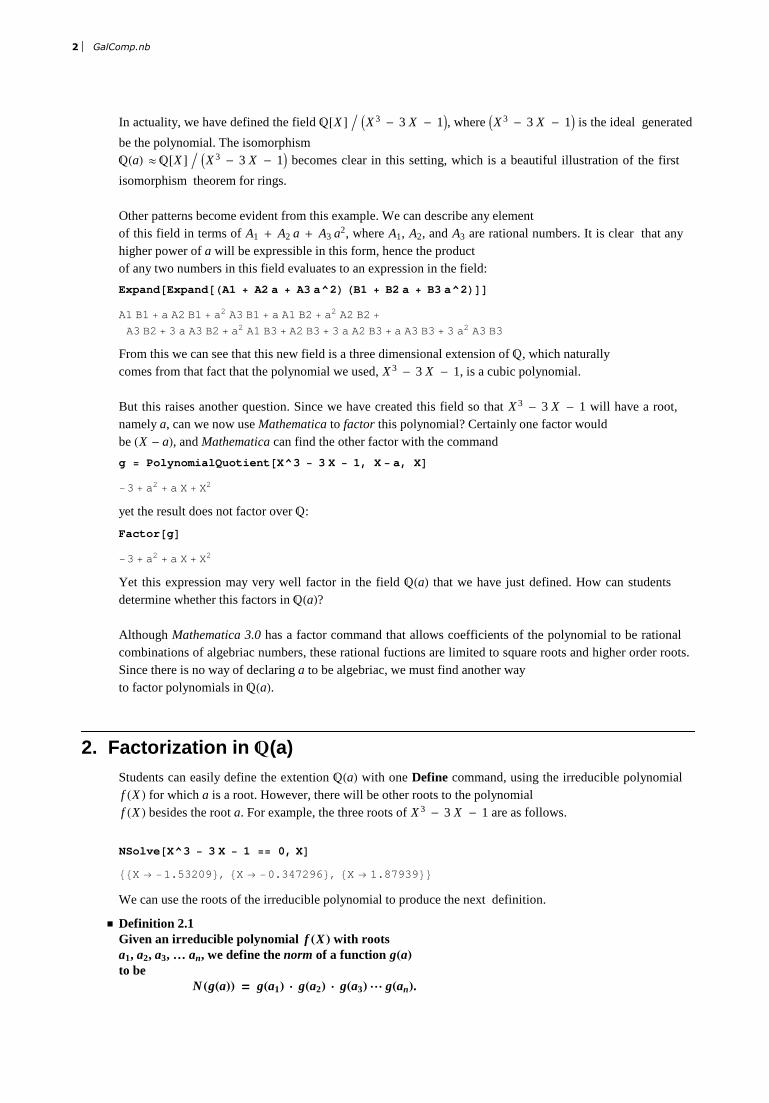
In actuality, we have defined the field Q@X D � IX 3 - 3 X - 1M, where IX 3 - 3 X - 1M is the ideal generated

be the polynomial. The isomorphismQHaL » Q@X D � IX 3 - 3 X - 1M becomes clear in this setting, which is a beautiful illustration of the first

isomorphism theorem for rings.

Other patterns become evident from this example. We can describe any elementof this field in terms of A1 + A2 a + A3 a2, where A1, A2, and A3 are rational numbers. It is clear that anyhigher power of a will be expressible in this form, hence the productof any two numbers in this field evaluates to an expression in the field:

which defines all powers of a recursively. Thus, Mathematica will quickly simplify a9 to 27 a2 + 90 a + 28.In like manner we can define QHaL for any algebraic number a.

In actuality, we have defined the field Q@X D � IX 3 - 3 X - 1M, where IX 3 - 3 X - 1M is the ideal generated

be the polynomial. The isomorphismQHaL » Q@X D � IX 3 - 3 X - 1M becomes clear in this setting, which is a beautiful illustration of the first

isomorphism theorem for rings.

Other patterns become evident from this example. We can describe any elementof this field in terms of A1 + A2 a + A3 a2, where A1, A2, and A3 are rational numbers. It is clear that anyhigher power of a will be expressible in this form, hence the productof any two numbers in this field evaluates to an expression in the field:

Expand@Expand@HA1 + A2 a + A3 a^2L HB1 + B2 a + B3 a^2LDD

A1 B1 + a A2 B1 + a2 A3 B1 + a A1 B2 + a2 A2 B2 +

A3 B2 + 3 a A3 B2 + a2 A1 B3 + A2 B3 + 3 a A2 B3 + a A3 B3 + 3 a2 A3 B3

From this we can see that this new field is a three dimensional extension of Q, which naturallycomes from that fact that the polynomial we used, X 3 - 3 X - 1, is a cubic polynomial.

But this raises another question. Since we have created this field so that X 3 - 3 X - 1 will have a root,namely a, can we now use Mathematica to factor this polynomial? Certainly one factor wouldbe HX - aL, and Mathematica can find the other factor with the command

g = PolynomialQuotient@X^3 - 3 X - 1, X - a, XD

-3 + a2+ a X + X2

yet the result does not factor over Q:

Factor@gD

-3 + a2+ a X + X2

Yet this expression may very well factor in the field QHaL that we have just defined. How can studentsdetermine whether this factors in QHaL?

Although Mathematica 3.0 has a factor command that allows coefficients of the polynomial to be rationalcombinations of algebriac numbers, these rational fuctions are limited to square roots and higher order roots.Since there is no way of declaring a to be algebriac, we must find another wayto factor polynomials in QHaL.

2. Factorization in Q(a)Students can easily define the extention QHaL with one Define command, using the irreducible polynomialf HX L for which a is a root. However, there will be other roots to the polynomialf HX L besides the root a. For example, the three roots of X 3 - 3 X - 1 are as follows.

NSolve@X^3 - 3 X - 1 == 0, XD

88X ® -1.53209<, 8X ® -0.347296<, 8X ® 1.87939<<

We can use the roots of the irreducible polynomial to produce the next definition.

� Definition 2.1Given an irreducible polynomial f HXL with rootsa1, a2, a3, … an, we define the norm of a function gHaLto be N HgHaLL = gHa1L × gHa2L × gHa3L º gHanL.For example, the norm of gHaL defined above can be computed inMathematica.

2 GalComp.nb

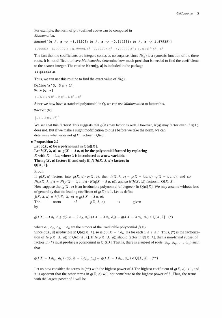
For example, the norm of gHaL defined above can be computed inMathematica.

Expand@Hg �. a -> -1.53209L Hg �. a -> -0.347296L Hg �. a -> 1.87939LD

1.00003 + 6.00007 X + 8.99996 X2- 2.00004 X3

- 5.99999 X4+ 4. ´ 10-6 X5

+ X6

The fact that the coefficients are integers comes as no surprise, since NHgL is a symetric function of the threeroots. It is not difficult to have Mathematica determine how much precision is needed to find the coefficientsto the nearest integer. The routine Norm[g, a] is included in the package

<< galois.m

Thus, we can use this routine to find the exact value of NHgL.Define@a^3, 3 a + 1DNorm@g, aD

1 + 6 X + 9 X2- 2 X3

- 6 X4+ X6

Since we now have a standard polynomial in Q, we can use Mathematica to factor this.

Factor@%D

I-1 - 3 X + X3M2

We see that this factors! This suggests that gHX L may factor as well. However, NHgL may factor even if gHX Ldoes not. But if we make a slight modification to gHX L before we take the norm, we candetermine whether or not gHX L factors in QHaL.

� Proposition 2.2Let gHX , aL be a polynomial in QHaL@XD. Let hHX , Λ, aL = gHX - Λ a, aL be the polynomial formed by replacingX with X - Λ a, where Λ is introduced as a new variable.Then gHX , aL factors if, and only if, N HhHX , Λ, aLL factors in Q@X , ΛD.

Proof:If gHX , aL factors into pHX , aL × q HX , aL, then hHX , Λ, aL = pHX - Λ a, aL × qHX - Λ a, aL, and soNHhHX , Λ, aLL = NHpHX - Λ a, aLL × NHqHX - Λ a, aLL, and so NHhHX , ΛLL factors in Q@X , ΛD. Now suppose that gHX , aL is an irreducible polynomial of degree r in QHaL@X D. We may assume without lossof generality that the leading coefficent of gHX L is 1. Let us define jHX , Λ, aL = hHΛ X , Λ, aL = gHΛ X - Λ a, aL.The norm of jHX , Λ, aL is givenby

gHΛ X - Λ a1, a1L × gHΛ X - Λ a2, a2L × HΛ X - Λ a3, a3L º gHΛ X - Λ an, anL Ε Q@X , ΛD (*)

where a1, a2, a3, … an are the n roots of the irreducible polynomial f HX L. Since gHX , aL irreducible in QHaL@X , ΛD, so is gHΛ X - Λ ai, aiL for each 1 £ i £ n. Thus, (*) is the factoriza-tion of NH jHX , Λ, aLL in QHaL@X , ΛD. If NH jHX , Λ, aLL should factor in Q@X , ΛD, then a non-trivial subset offactors in (*) must produce a polynomial in Q[X,Λ]. That is, there is a subset of roots 8ak1

, ak2, …, akm < such

that

gHΛ X - Λ ak1, ak1

L × gHΛ X - Λ ak2, ak2

L º gHΛ X - Λ akm , akm L Ε Q@X , ΛD. (**)

Let us now consider the terms in (**) with the highest power of Λ.The highest coefficient of gHX , aL is 1, andit is apparent that the other terms in gHX , aL will not contribute to the highest power of Λ. Thus, the termswith the largest power of Λ will be

Λr m × HX - ak1Lr × HX - ak2

Lrº HX - akm Lr.

Thus, @HX - ak1L HX - ak2

L ºHX - akm LD r Ε Q@X D. But since Q is of characteristic 0, we can say that

HX - ak1L HX - ak2

L ºHX - akm L Ε Q@X D. But f HX L is an irreducible polynomial of degree n containing the

same roots. Thus, m = n, and so NH jHX , Λ, aLL is irreducible in Q@X , ΛD. Since NHhHX , Λ, aLL is merelyNH jHX , Λ, aLL , replacing X with X � Λ, we have that NHhHX , Λ, aLL is also irreducible in Q@X , ΛD. �

GalComp.nb 3

Proof:If gHX , aL factors into pHX , aL × q HX , aL, then hHX , Λ, aL = pHX - Λ a, aL × qHX - Λ a, aL, and soNHhHX , Λ, aLL = NHpHX - Λ a, aLL × NHqHX - Λ a, aLL, and so NHhHX , ΛLL factors in Q@X , ΛD. Now suppose that gHX , aL is an irreducible polynomial of degree r in QHaL@X D. We may assume without lossof generality that the leading coefficent of gHX L is 1. Let us define jHX , Λ, aL = hHΛ X , Λ, aL = gHΛ X - Λ a, aL.The norm of jHX , Λ, aL is givenby

gHΛ X - Λ a1, a1L × gHΛ X - Λ a2, a2L × HΛ X - Λ a3, a3L º gHΛ X - Λ an, anL Ε Q@X , ΛD (*)

where a1, a2, a3, … an are the n roots of the irreducible polynomial f HX L. Since gHX , aL irreducible in QHaL@X , ΛD, so is gHΛ X - Λ ai, aiL for each 1 £ i £ n. Thus, (*) is the factoriza-tion of NH jHX , Λ, aLL in QHaL@X , ΛD. If NH jHX , Λ, aLL should factor in Q@X , ΛD, then a non-trivial subset offactors in (*) must produce a polynomial in Q[X,Λ]. That is, there is a subset of roots 8ak1

, ak2, …, akm < such

that

gHΛ X - Λ ak1, ak1

L × gHΛ X - Λ ak2, ak2

L º gHΛ X - Λ akm , akm L Ε Q@X , ΛD. (**)

Let us now consider the terms in (**) with the highest power of Λ.The highest coefficient of gHX , aL is 1, andit is apparent that the other terms in gHX , aL will not contribute to the highest power of Λ. Thus, the termswith the largest power of Λ will be

Λr m × HX - ak1Lr × HX - ak2

Lrº HX - akm Lr.

Thus, @HX - ak1L HX - ak2

L ºHX - akm LD r Ε Q@X D. But since Q is of characteristic 0, we can say that

HX - ak1L HX - ak2

L ºHX - akm L Ε Q@X D. But f HX L is an irreducible polynomial of degree n containing the

same roots. Thus, m = n, and so NH jHX , Λ, aLL is irreducible in Q@X , ΛD. Since NHhHX , Λ, aLL is merelyNH jHX , Λ, aLL , replacing X with X � Λ, we have that NHhHX , Λ, aLL is also irreducible in Q@X , ΛD. �

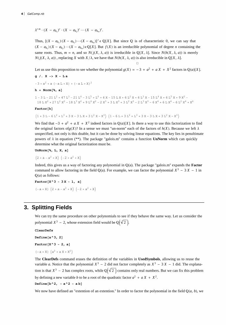
Let us use this proposition to see whether the polynomial gHX L = - 3 + a2 + a X + X 2 factors in QHaL@X D.g �. X -> X - L a

-3 + a2+ a H-a L + XL + H-a L + XL2

h = Norm@%, aD

1 - 3 L - 21 L2+ 47 L3

- 21 L4- 3 L5

+ L6+ 6 X - 15 L X + 6 L2 X + 6 L3 X - 15 L4 X + 6 L5 X + 9 X2

-

18 L X2+ 27 L2 X2

- 18 L3 X2+ 9 L4 X2

- 2 X3+ 3 L X3

+ 3 L2 X3- 2 L3 X3

- 6 X4+ 6 L X4

- 6 L2 X4+ X6

Factor@hD

I1 + 3 L - 6 L2+ L3

+ 3 X - 3 L X + 3 L2 X - X3M I1 - 6 L + 3 L2+ L3

+ 3 X - 3 L X + 3 L2 X - X3M

We find that -3 + a2 + a X + X 2 indeed factors in QHaL@X D. Is there a way to use this factorization to findthe original factors ofgHX L? In a sense we must "un-norm'' each of the factors of hHX L. Because we left Λunspecified, not only is this doable, but it can be done by solving linear equations. The key lies in penultimatepowers of Λ in equation (**). The package "galois.m'' contains a function UnNorm which can quicklydetermine what the original factorization must be.

UnNorm@%, L, X, aD

I2 + a - a2+ XM I-2 + a2

+ XM

Indeed, this gives us a way of factoring any polynomial in Q(a). The package "galois.m'' expands the Factorcommand to allow factoring in the field Q(a). For example, we can factor the polynomial X 3 - 3 X - 1 inQHaL as follows:

Factor@X^3 - 3 X - 1, aD

H-a + XL I2 + a - a2+ XM I-2 + a2

+ XM

3. Splitting FieldsWe can try the same procedure on other polynomials to see if they behave the same way. Let us consider the

polynomial X 3 - 2, whose extension field would be QJ 23 N.

ClearDefs

Define@a^3, 2D

Factor@X^3 - 2, aD

H-a + XL Ia2+ a X + X2M

The ClearDefs command erases the definition of the variables in UsedSymbols, allowing us to reuse thevariable a. Notice that the polynomial X 3 - 2 did not factor completely as X 3 - 3 X - 1 did. The explana-

tion is that X 3 - 2 has complex roots, while QJ 23 N contains only real numbers. But we can fix this problem

by defining a new variable b to be a root of the quadratic factor a2 + a X + X 2.

Define@b^2, - a^2 - a bD

We now have defined an "extention of an extention.'' In order to factor the polynomial in the field QHa, bL, wewill apply a shortcut. We will use the following theorem found in many abstract algebra books.

4 GalComp.nb

We now have defined an "extention of an extention.'' In order to factor the polynomial in the field QHa, bL, wewill apply a shortcut. We will use the following theorem found in many abstract algebra books.

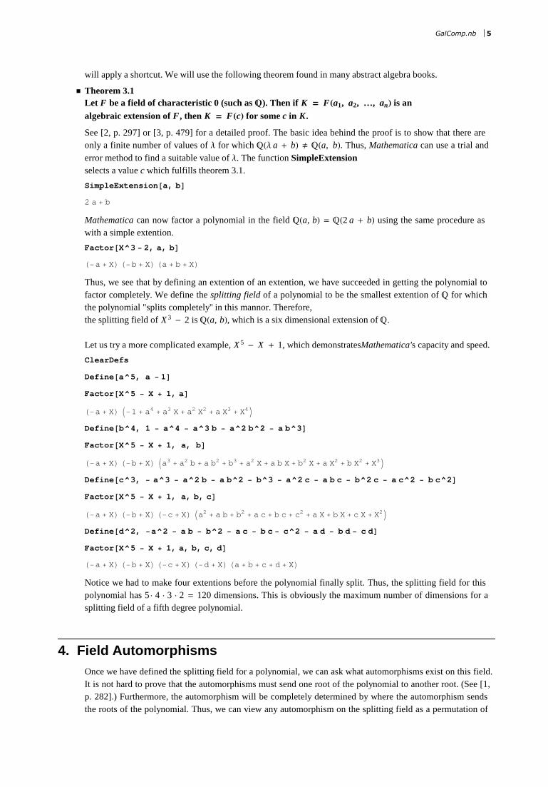
� Theorem 3.1Let F be a field of characteristic 0 (such as Q). Then if K = FHa1, a2, …, anL is an algebraic extension of F, then K = FHcL for some c in K.

See [2, p. 297] or [3, p. 479] for a detailed proof. The basic idea behind the proof is to show that there areonly a finite number of values of Λ for which QHΛ a + bL ¹ QHa, bL. Thus, Mathematica can use a trial anderror method to find a suitable value of Λ. The function SimpleExtensionselects a value c which fulfills theorem 3.1.

SimpleExtension@a, bD

2 a + b

Mathematica can now factor a polynomial in the field QHa, bL = QH2 a + bL using the same procedure aswith a simple extention.

Factor@X^3 - 2, a, bD

H-a + XL H-b + XL Ha + b + XL

Thus, we see that by defining an extention of an extention, we have succeeded in getting the polynomial tofactor completely. We define the splitting field of a polynomial to be the smallest extention of Q for whichthe polynomial "splits completely'' in this mannor. Therefore,the splitting field of X 3 - 2 is QHa, bL, which is a six dimensional extension of Q.

Let us try a more complicated example, X 5 - X + 1, which demonstratesMathematica's capacity and speed.

ClearDefs

Define@a^5, a - 1D

Factor@X^5 - X + 1, aD

H-a + XL I-1 + a4+ a3 X + a2 X2

+ a X3+ X4M

Define@b^4, 1 - a^4 - a^3 b - a^2 b^2 - a b^3D

Factor@X^5 - X + 1, a, bD

H-a + XL H-b + XL Ia3+ a2 b + a b2

+ b3+ a2 X + a b X + b2 X + a X2

+ b X2+ X3M

Define@c^3, - a^3 - a^2 b - a b^2 - b^3 - a^2 c - a b c - b^2 c - a c^2 - b c^2D

Factor@X^5 - X + 1, a, b, cD

H-a + XL H-b + XL H-c + XL Ia2+ a b + b2

+ a c + b c + c2+ a X + b X + c X + X2M

Define@d^2, -a^2 - a b - b^2 - a c - b c - c^2 - a d - b d - c dD

Factor@X^5 - X + 1, a, b, c, dD

H-a + XL H-b + XL H-c + XL H-d + XL Ha + b + c + d + XL

Notice we had to make four extentions before the polynomial finally split. Thus, the splitting field for thispolynomial has 5 × 4 × 3 × 2 = 120 dimensions. This is obviously the maximum number of dimensions for asplitting field of a fifth degree polynomial.

4. Field AutomorphismsOnce we have defined the splitting field for a polynomial, we can ask what automorphisms exist on this field.It is not hard to prove that the automorphisms must send one root of the polynomial to another root. (See [1,p. 282].) Furthermore, the automorphism will be completely determined by where the automorphism sendsthe roots of the polynomial. Thus, we can view any automorphism on the splitting field as a permutation ofthe roots of the polynomial.

How can we determine whether a given permutation of the roots represents an automorphism? We can haveMathematica help us! Let us choose the polynomial X 5 - 5 X + 12 to illustrate the process.

GalComp.nb 5

Once we have defined the splitting field for a polynomial, we can ask what automorphisms exist on this field.It is not hard to prove that the automorphisms must send one root of the polynomial to another root. (See [1,p. 282].) Furthermore, the automorphism will be completely determined by where the automorphism sendsthe roots of the polynomial. Thus, we can view any automorphism on the splitting field as a permutation ofthe roots of the polynomial.

How can we determine whether a given permutation of the roots represents an automorphism? We can haveMathematica help us! Let us choose the polynomial X 5 - 5 X + 12 to illustrate the process.

ClearDefs

Define@a^5, 5 a - 12D

Factor@X^5 - 5 X + 12, aD

H-a + XL 2 -

5 a

4-

a2

4-

a3

4-

a4

4+ X +

3 a X

4-

a2 X

4-

a3 X

4-

a4 X

4+ X2

-1 -

a

2-

a3

2- X +

a X

4+

a2 X

4+

a3 X

4+

a4 X

4+ X2

We can let b be a root of the last factor, and try the factorization again.

Define@b^2, 1 + a � 2 + a^3 � 2 + b - a b � 4 - a^2 b � 4 - a^3 b � 4 - a^4 b � 4D

Factor@X^5 - 5 X + 12, a, bD

H-a + XL H-b + XL -1 +

a

4+

a2

4+

a3

4+

a4

4+ b + X

3

2+

a

4-

a2

4-

a3

4-

a4

4-

b

2-

a b

2+ X -

1

2+

a

2+

b

2+

a b

2+ X

It is natural to label the three other roots of this polynomial as c, d, and e.

c = 1 - a � 4 - a^2 � 4 - a^3 � 4 - a^4 � 4 - b;

d = -3 � 2 - a � 4 + a^2 � 4 + a^3 � 4 + a^4 � 4 + b � 2 + a b � 2;

e = 1 � 2 - a � 2 - b � 2 - a b � 2;

In order to define an automorphism on this splitting field, we only have to define where a and b are sent to,and the other three roots will follow suit. It is easy to define a homomorphism in Mathematica. The followingcreates the command Homomorph[F] which defines F to be a homomorphism.

Homomorph@F_SymbolD := Module@8a, b<,

UsedSymbols = Union@UsedSymbols, 8F<D;

ClearAll@FD;

F@a_ b_D := FixedPoint@Expand, F@aD F@bDD;

F@a_ + b_D := F@aD + F@bD;

F@a_ ^b_IntegerD := FixedPoint@Expand, F@aD^bD;

F@a_IntegerD := a;

F@a_RationalD := a;D

For example, we can easily define a homomorphism which sends a to b, and sends b back to a.

Homomorph@FD

F@aD := b

F@bD := a

The command CheckHomo in the package "galois.m'' can confirm for us that this is indeed a homomorphismon QHa, bL.CheckHomo@F, 8a, b<D

True

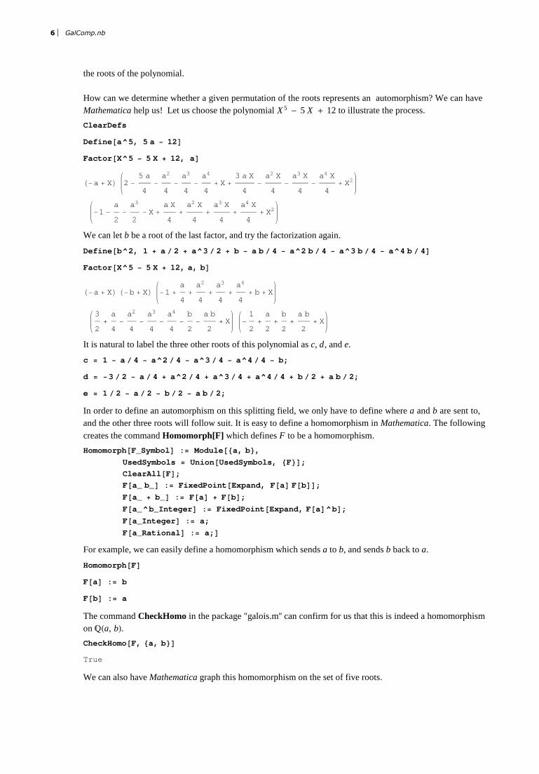
We can also have Mathematica graph this homomorphism on the set of five roots.

6 GalComp.nb

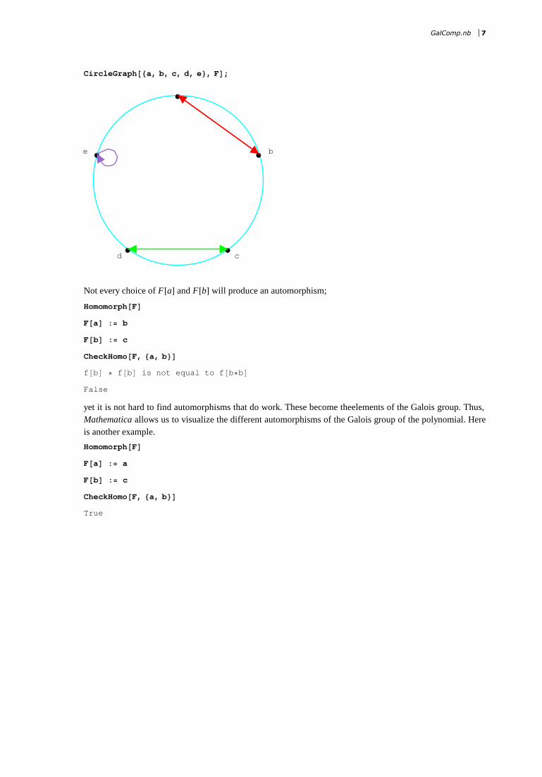
CircleGraph@8a, b, c, d, e<, FD;

Ł

ŁŁ

Ł

Ł

a

b

cd

e

Not every choice of F@aD and F@bD will produce an automorphism;

Homomorph@FD

F@aD := b

F@bD := c

CheckHomo@F, 8a, b<D

f@bD * f@bD is not equal to f@b*bD

False

yet it is not hard to find automorphisms that do work. These become theelements of the Galois group. Thus,Mathematica allows us to visualize the different automorphisms of the Galois group of the polynomial. Hereis another example.

Homomorph@FD

F@aD := a

F@bD := c

CheckHomo@F, 8a, b<D

True

GalComp.nb 7

CircleGraph@8a, b, c, d, e<, FD;

Ł

ŁŁ

Ł

Ł

a

b

cd

e

From these two elements of the Galois group, we can actually produce the entire Galois group ofX 5 - 5 X + 12. We will develop a quick way to produce these elements in the next section.

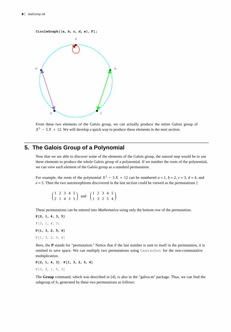
5. The Galois Group of a PolynomialNow that we are able to discover some of the elements of the Galois group, the natural step would be to usethese elements to produce the whole Galois group of a polynomial. If we number the roots of the polynomial,we can view each element of the Galois group as a standard permutation.

For example, the roots of the polynomial X 5 - 5 X + 12 can be numbered a = 1, b = 2, c = 3, d = 4, ande = 5. Then the two automorphisms discovered in the last section could be viewed as the permutations ]

1 2 3 4 5

2 1 4 3 5 and

1 2 3 4 5

1 3 2 5 4.

These permutations can be entered into Mathematica using only the bottom row of the permutation.

P@2, 1, 4, 3, 5D

P@2, 1, 4, 3D

P@1, 3, 2, 5, 4D

P@1, 3, 2, 5, 4D

Here, the P stands for "permutation.'' Notice that if the last number is sent to itself in the permutation, it isomitted to save space. We can multiply two permutations using CenterDot for the non-commutativemultiplication.

P@2, 1, 4, 3D × P@1, 3, 2, 5, 4D

P@2, 4, 1, 5, 3D

The Group command, which was described in [4], is also in the "galios.m'' package. Thus, we can find thesubgroup of S5 generated by these two permutations as follows:

8 GalComp.nb

Group@8P@2, 1, 4, 3D, P@1, 3, 2, 5, 4D<D

8P@D, P@2, 1, 4, 3D, P@1, 3, 2, 5, 4D, P@3, 1, 5, 2, 4D, P@2, 4, 1, 5, 3D,

P@4, 2, 5, 1, 3D, P@3, 5, 1, 4, 2D, P@5, 3, 4, 1, 2D, P@4, 5, 2, 3, 1D, P@5, 4, 3, 2, 1D<

Since the splitting field of X 5 - 5 X + 12 is 10 dimensional, we would expect the Galois group to have 10elements. Since Mathematica has found 10 elements in the Galois group, we have found all of them.

Which group is this isomorphic to? It is obvious that none of these elements is of order 10. Thus, the groupcannot be isomorphic to Z10. The only other group of order 10 is D5, so this group is isomorphic to D5. Notethat [5] claims the Galois group is F20, which is wrong.

Let us try one more example---the polynomial X 8 - 24 X 6 + 144 X 4 - 288 X 2 + 144. We can first notethat this polynomial is irreducible over the rational numbers.

ClearDefs

Factor@X^8 - 24 X^6 + 144 X^4 - 288 X^2 + 144D

144 - 288 X2+ 144 X4

- 24 X6+ X8

We can define a to be a root of this polynomial, and factor it over QHaL.Define@a^8, 24 a^6 - 144 a^4 + 288 a^2 - 144D

Factor@X^8 - 24 X^6 + 144 X^4 - 288 X^2 + 144, aD

H-a + XL Ha + XL -3 a +

3 a3

2-

a5

12+ X 3 a -

3 a3

2+

a5

12+ X 10 a -

17 a3

2+

11 a5

6-

a7

12+ X

-a -

5 a3

2+

5 a5

6-

a7

24+ X a +

5 a3

2-

5 a5

6+

a7

24+ X -10 a +

17 a3

2-

11 a5

6+

a7

12+ X

As we can see, the polynomial factors completely in QHaL. The roots can be given as ±a, ±b, ±c, and ±d,where

b = a + 5 a^3 � 2 - 5 a^5 � 6 + a^7 � 24;

c = 3 a - 3 a^3 � 2 + a^5 � 12;

d = 10 a - 17 a^3 � 2 + 11 a^5 � 6 - a^7 � 12;

which are all expressed in terms of a. Thus, an automorphism of the splitting field will be completely deter-mined by which root a is sent to. Suppose that a is sent to b.

Homomorph@FD

F@aD := b

CheckHomo@F, 8a<D

True

GalComp.nb 9

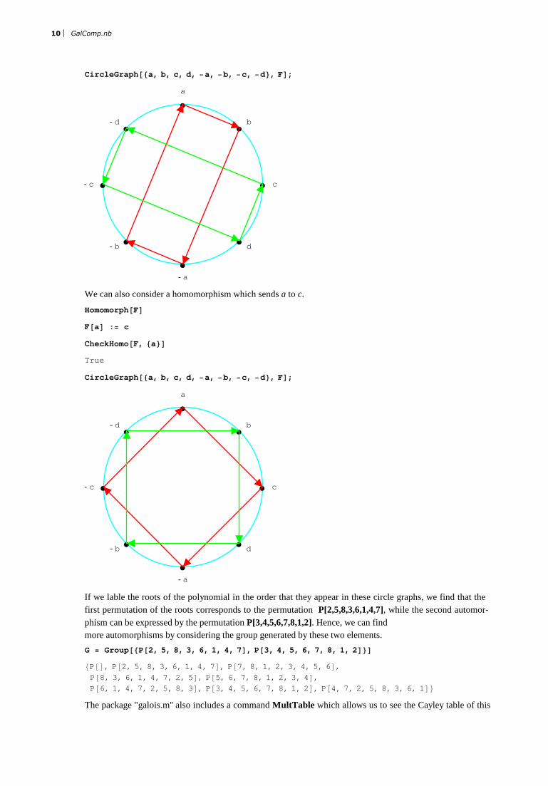
CircleGraph@8a, b, c, d, -a, -b, -c, -d<, FD;

Ł

Ł

Ł

Ł

Ł

Ł

Ł

Ł

a

-a

b

c

d-b

-c

-d

We can also consider a homomorphism which sends a to c.

Homomorph@FD

F@aD := c

CheckHomo@F, 8a<D

True

CircleGraph@8a, b, c, d, -a, -b, -c, -d<, FD;

Ł

Ł

Ł

Ł

Ł

Ł

Ł

Ł

a

-a

b

c

d-b

-c

-d

If we lable the roots of the polynomial in the order that they appear in these circle graphs, we find that thefirst permutation of the roots corresponds to the permutation P[2,5,8,3,6,1,4,7], while the second automor-phism can be expressed by the permutation P[3,4,5,6,7,8,1,2]. Hence, we can findmore automorphisms by considering the group generated by these two elements.

G = Group@8P@2, 5, 8, 3, 6, 1, 4, 7D, P@3, 4, 5, 6, 7, 8, 1, 2D<D

8P@D, P@2, 5, 8, 3, 6, 1, 4, 7D, P@7, 8, 1, 2, 3, 4, 5, 6D,

P@8, 3, 6, 1, 4, 7, 2, 5D, P@5, 6, 7, 8, 1, 2, 3, 4D,

P@6, 1, 4, 7, 2, 5, 8, 3D, P@3, 4, 5, 6, 7, 8, 1, 2D, P@4, 7, 2, 5, 8, 3, 6, 1D<

The package "galois.m'' also includes a command MultTable which allows us to see the Cayley table of thisgroup of permutations.

10 GalComp.nb

The package "galois.m'' also includes a command MultTable which allows us to see the Cayley table of thisgroup of permutations.

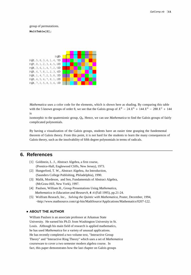
MultTable@GD;

P@DP@2,5,8,3,6,1,4,7DP@7,8,1,2,3,4,5,6DP@8,3,6,1,4,7,2,5DP@5,6,7,8,1,2,3,4DP@6,1,4,7,2,5,8,3DP@3,4,5,6,7,8,1,2DP@4,7,2,5,8,3,6,1D

Mathematica uses a color code for the elements, which is shown here as shading. By comparing this tablewith the 5 known groups of order 8, we see that the Galois group of X 8 - 24 X 6 + 144 X 4 - 288 X 2 + 144is isomorphic to the quaternionic group, Q8. Hence, we can use Mathematica to find the Galois groups of fairlycomplicated polynomials.

By having a visualization of the Galois groups, students have an easier time grasping the fundementaltheorem of Galois theory. From this point, it is not hard for the students to learn the many consequences ofGalois theory, such as the insolvability of fifth degree polynomials in terms of radicals.

6. References[1] Goldstein, L. J., Abstract Algebra, a first course, (Prentice-Hall, Englewood Cliffs, New Jersey), 1973.[2] Hungerford, T. W., Abstract Algebra, An Introduction, (Saunders College Publishing, Philadelphia), 1990.[3] Malik, Mordeson, and Sen, Fundamentals of Abstract Algebra, (McGraw-Hill, New York), 1997.[4] Paulsen, William H., Group Presentations Using Mathematica, Mathematica in Education and Research, 4 :4 (Fall 1995), pp.21-24.[5] Wolfram Reseach, Inc., Solving the Quintic with Mathematica, Poster, December, 1994, ¬http://www.mathsource.com/cgi-bin/MathSource/Applications/Mathematics/0207-122.

� ABOUT THE AUTHOR

William Paulsen is an associate professor at Arkansas State University. He earned his Ph.D. from Washington University in St. Louis. Although his main field of research is applied mathematics,he has used Mathematica for a variety of unusual applications. He has recently completed a two volume text, "Interactive Group Theory" and "Interactive Ring Theory" which uses a set of Mathematicacourseware to cover a two semester modern algebra course. In fact, this paper demonstrates how the last chapter on Galois groupswas implemented into Mathematica. The two volume text has yet to be accepted for publication. William Paulsen Department of Mathematics and Computer ScienceP. O. Box 70State University, AR 72467wpaulsen@caddo.astate.edu

GalComp.nb 11

William Paulsen is an associate professor at Arkansas State University. He earned his Ph.D. from Washington University in St. Louis. Although his main field of research is applied mathematics,he has used Mathematica for a variety of unusual applications. He has recently completed a two volume text, "Interactive Group Theory" and "Interactive Ring Theory" which uses a set of Mathematicacourseware to cover a two semester modern algebra course. In fact, this paper demonstrates how the last chapter on Galois groupswas implemented into Mathematica. The two volume text has yet to be accepted for publication. William Paulsen Department of Mathematics and Computer ScienceP. O. Box 70State University, AR 72467wpaulsen@caddo.astate.edu

� ELECTRONIC SUBSCRIPTIONS

Included in the distribution for each electronic subscription are the files galois.m and GalComp.nb

containing Mathematica code for the material described in this article.

12 GalComp.nb