COMPSCI220 Review & Questions

Ulrich Speidel (ulrich@cs.auckland.ac.nz)

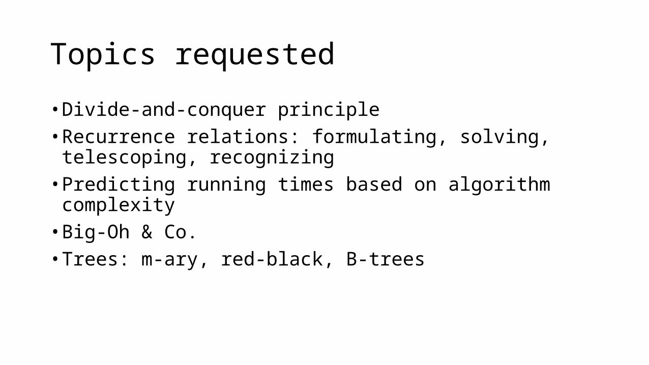
Topics requested

• Divide-and-conquer principle• Recurrence relations: formulating, solving, telescoping, recognizing• Predicting running times based on algorithm complexity• Big-Oh & Co.• Trees: m-ary, red-black, B-trees

Divide and conquer

• Basic idea: You have a big and potentially messy problem (such as sorting a list of ten million numbers, or traversing a large graph that I don’t know in advance, or…). Lots of possible strategies and solutions.• Divide and conquer: Identify how to break up the big problem into

(progressively) smaller ones that you can solve easily.• Examples:

• Mergesort: Divide up large list recursively into smaller ones that you can sort easily once they reach length 2 or 1. Then conquer by combining (merging) your small sorted lists into larger sorted lists. Quicksort is another similar example here.

• DFS: Divide problem by conquering a graph one tree at a time. In each tree divide problem further by performing the same sub-algorithm on each node you visit (mark node gray, check for white outneighbours, visit them recursively, mark node black). BFS is another example in this respect.

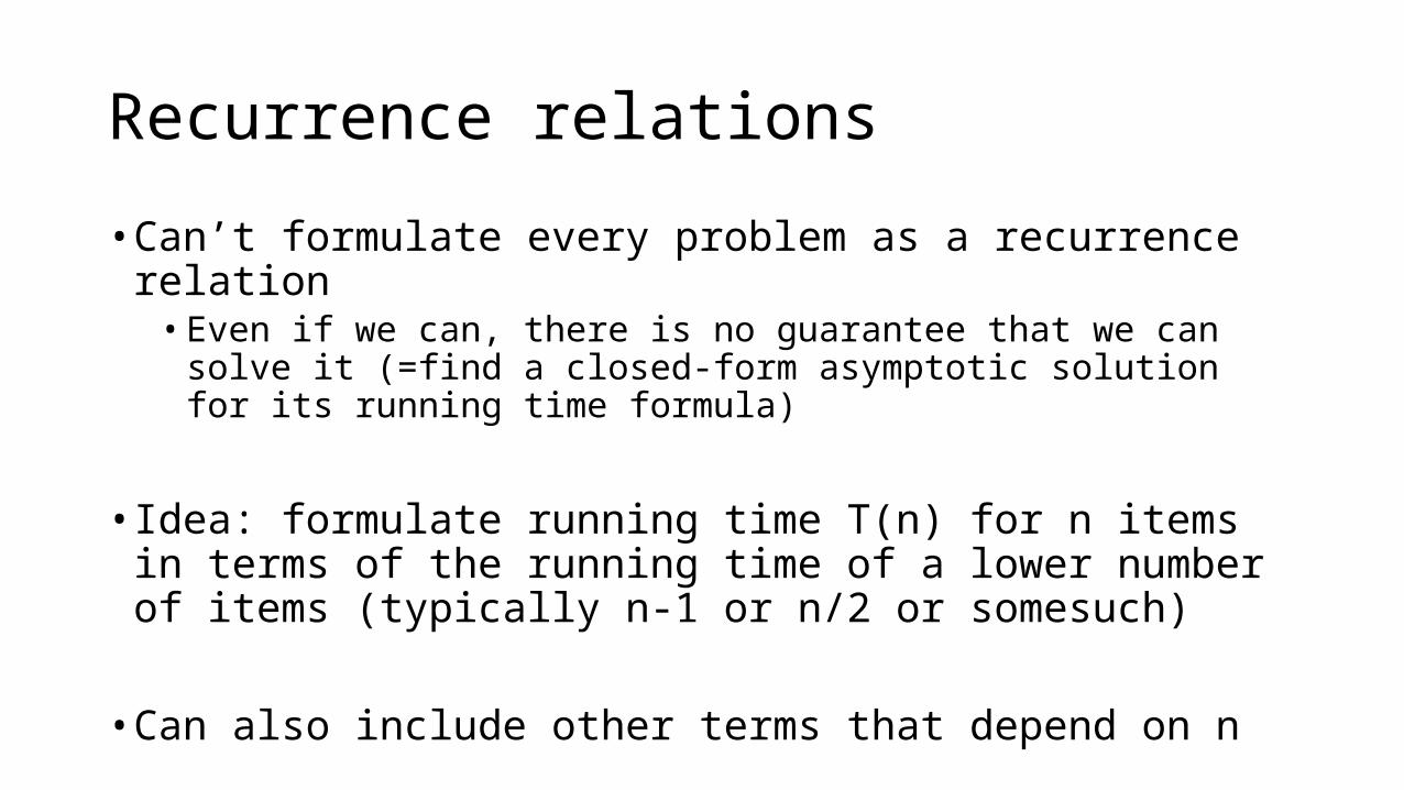
Recurrence relations

• Can’t formulate every problem as a recurrence relation• Even if we can, there is no guarantee that we can solve it (=find a closed-form

asymptotic solution for its running time formula)

• Idea: formulate running time T(n) for n items in terms of the running time of a lower number of items (typically n-1 or n/2 or somesuch)

• Can also include other terms that depend on n

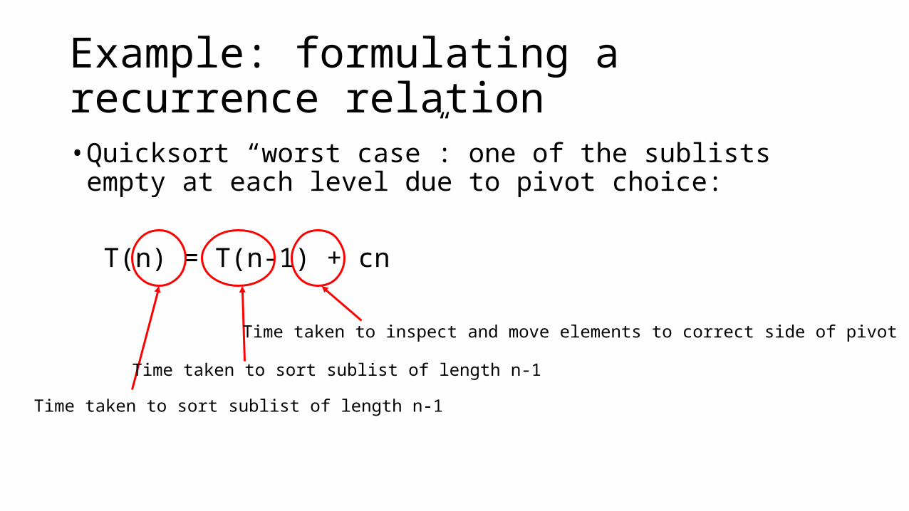
Example: formulating a recurrence relation• Quicksort “worst case”: one of the sublists empty at each level due to

pivot choice:

T(n) = T(n-1) + cn

Time taken to inspect and move elements to correct side of pivot

Time taken to sort sublist of length n-1

Time taken to sort sublist of length n-1

Exercise: formulating a recurrence relation

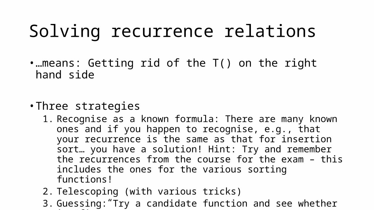
Solving recurrence relations

• …means: Getting rid of the T() on the right hand side

• Three strategies1. Recognise as a known formula: There are many known ones and if you

happen to recognise, e.g., that your recurrence is the same as that for insertion sort… you have a solution! Hint: Try and remember the recurrences from the course for the exam – this includes the ones for the various sorting functions!

2. Telescoping (with various tricks)3. Guessing: Try a candidate function and see whether it “fits”

Solving a recurrence relation by recognition

Remember the recurrence relation for quicksort?

Identify c=5 and then you know that the average case time complexity for quicksort is…?

1

0

2 )()(n

in cniTnT

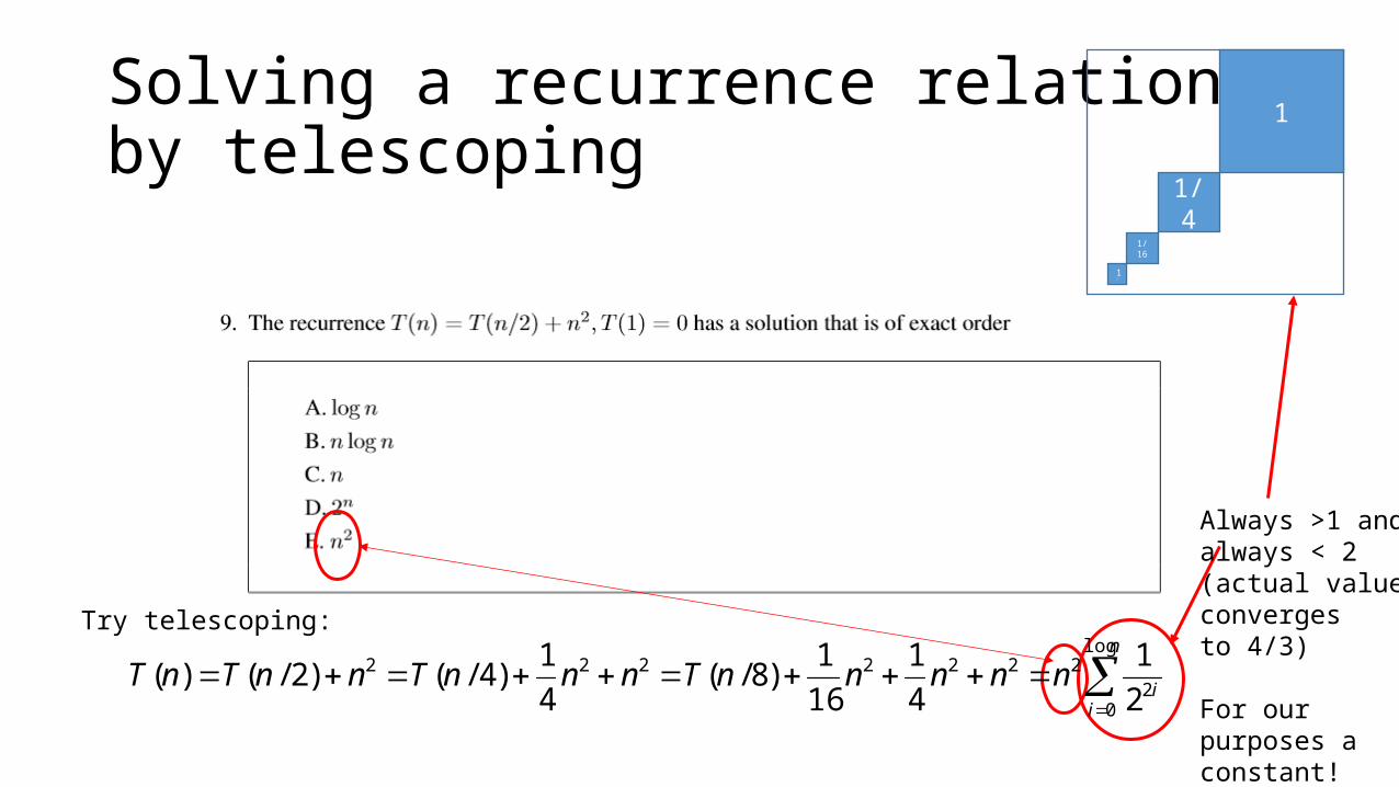
Solving a recurrence relation by telescoping

Try telescoping:

n

ii

nnnnnTnnnTnnTnTlog

02

2222222

2

1

4

1

16

1)8/(

4

1)4/()2/()(

Always >1 and always < 2(actual valueconverges to 4/3)

For our purposes a constant!

1

1/41/16

1/64

Telescoping

• Try and find some sort of regularity by substituting the recurrence relation for smaller n

• Being good at maths (or knowing someone who is) helps

• No guarantees!

Solving a recurrence relation by guessing• Guess that T(n) is 4n2/3 plus lower order terms

How do you check? Plug in the suspected asymptotic function (n2):

4n2/3 = 4(n/2)2/3+n2 gives 4n2/3 = n2/3+n2

If need be, divide the LHS of the equation by the RHS and ask what happens as n becomes really large. If you’ve guessed right, the result should converge to 1.

22

2

22

2

)2/()2/( nn

n

nn

n

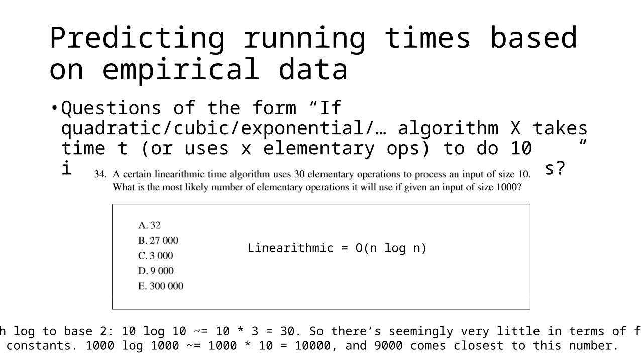
Predicting running times based on empirical data• Questions of the form “If quadratic/cubic/exponential/… algorithm X

takes time t (or uses x elementary ops) to do 10 items, how long does it take to do 100 items?”

Linearithmic = O(n log n)

Now, with log to base 2: 10 log 10 ~= 10 * 3 = 30. So there’s seemingly very little in terms of factors or additive constants. 1000 log 1000 ~= 1000 * 10 = 10000, and 9000 comes closest to this number.

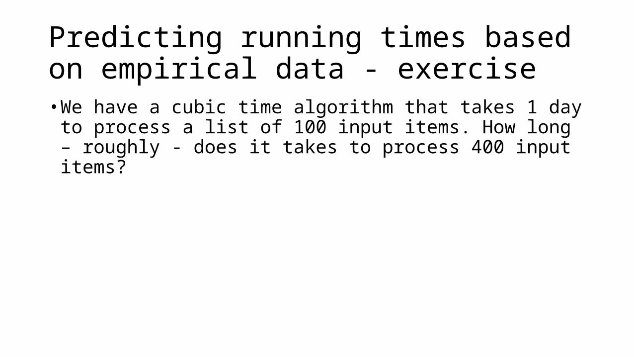
Predicting running times based on empirical data - exercise• We have a cubic time algorithm that takes 1 day to process a list of

100 input items. How long – roughly - does it takes to process 400 input items?

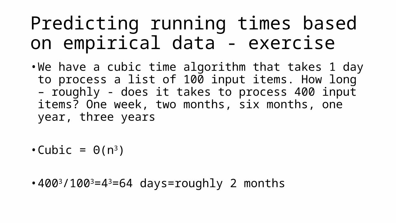
Predicting running times based on empirical data - exercise• We have a cubic time algorithm that takes 1 day to process a list of

100 input items. How long – roughly - does it takes to process 400 input items? One week, two months, six months, one year, three years

• Cubic = Θ(n3)

• 4003/1003=43=64 days=roughly 2 months

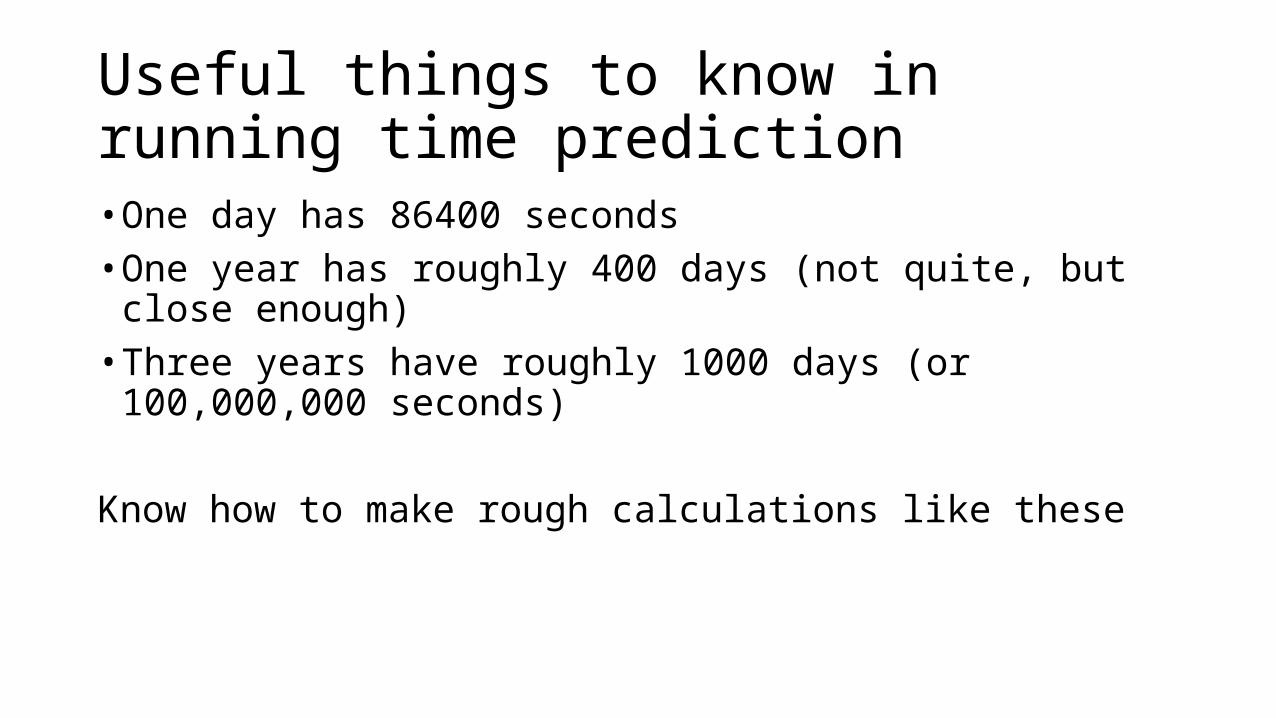
Useful things to know in running time prediction• One day has 86400 seconds• One year has roughly 400 days (not quite, but close enough)• Three years have roughly 1000 days (or 100,000,000 seconds)

Know how to make rough calculations like these

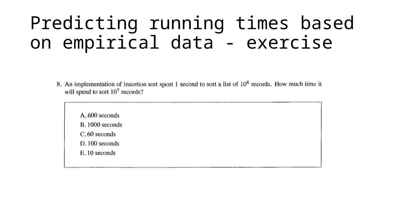
Predicting running times based on empirical data - exercise

17

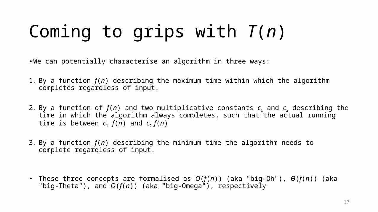
Coming to grips with T(n)

• We can potentially characterise an algorithm in three ways:

1. By a function f(n) describing the maximum time within which the algorithm completes regardless of input.

2. By a function of f(n) and two multiplicative constants c1 and c2 describing the time in which the algorithm always completes, such that the actual running time is between c1 f(n) and c2 f(n)

3. By a function f(n) describing the minimum time the algorithm needs to complete regardless of input.

• These three concepts are formalised as O(f(n)) (aka "big-Oh"), ϴ(f(n)) (aka "big-Theta"), and Ω(f(n)) (aka "big-Omega"), respectively

18

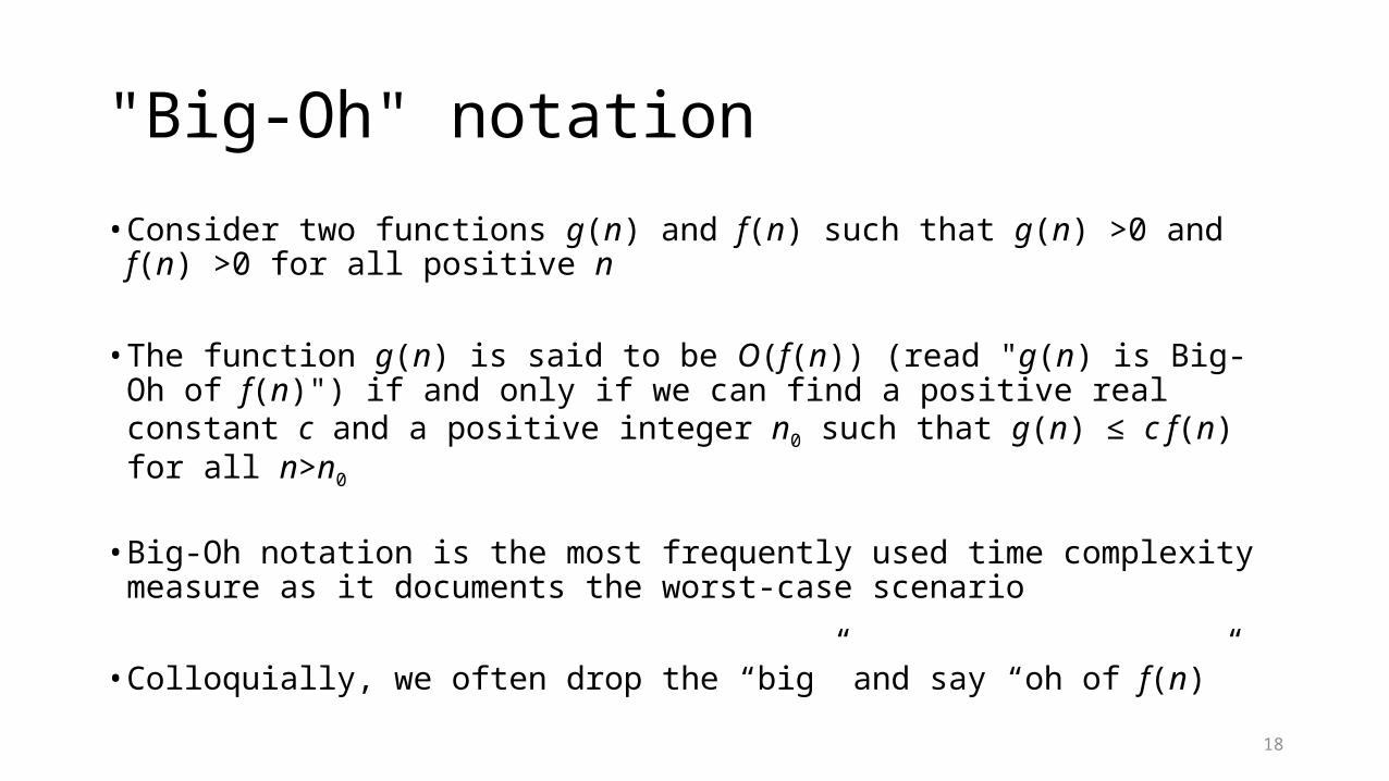
"Big-Oh" notation

• Consider two functions g(n) and f(n) such that g(n) >0 and f(n) >0 for all positive n

• The function g(n) is said to be O(f(n)) (read "g(n) is Big-Oh of f(n)") if and only if we can find a positive real constant c and a positive integer n0 such that g(n) ≤ c f(n) for all n>n0

• Big-Oh notation is the most frequently used time complexity measure as it documents the worst-case scenario

• Colloquially, we often drop the “big” and say “oh of f(n)”

19

Notes on Big-Oh

• Big-Oh describes an upper limit on asymptotic behaviour, that is a property that g(n) has for large n (n that are larger than some n0). As such it defines a class of functions that all exhibit this behaviour.

• It's not unique: for example, a linear algorithm is always O(n), but it is also O(n2), O(n3), O(en), etc. - O(f(n)) for any function f(n) that features a more rapid growth rate than n, in fact. Typically, we’ll be trying to quote the function with the lowest growth rate (i.e., O(n) for a linear algorithm)

• Multiplicative constants in f(n) are omitted, e.g., we normally do not write O(3n2) as it is the same as O(n2).

• Similarly, additive terms of a lower order are omitted: O(3n2 + 55n) is still just O(n2).

• Question to test your understanding: Why can we write O(n log n) without giving the base of the logarithm? (Hint: logax = logbx/logba).

20

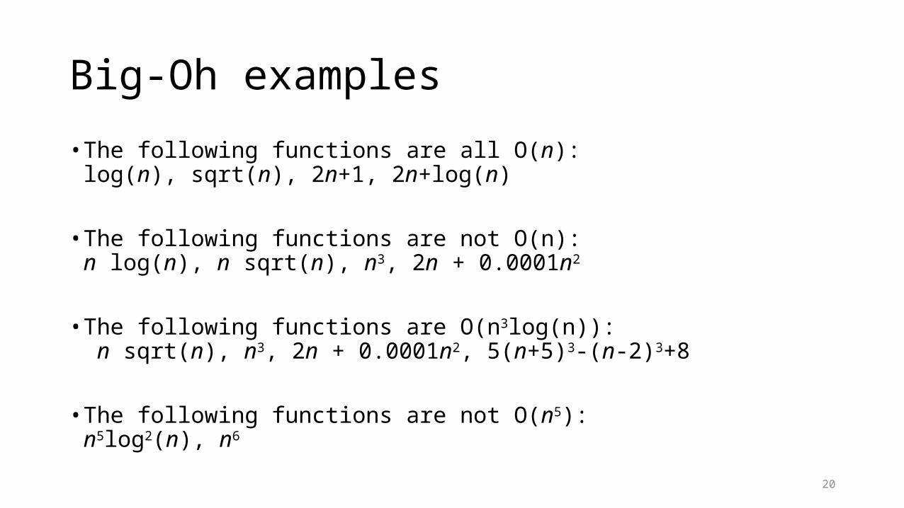
Big-Oh examples

• The following functions are all O(n):log(n), sqrt(n), 2n+1, 2n+log(n)

• The following functions are not O(n):n log(n), n sqrt(n), n3, 2n + 0.0001n2

• The following functions are O(n3log(n)): n sqrt(n), n3, 2n + 0.0001n2, 5(n+5)3-(n-2)3+8

• The following functions are not O(n5):n5log2(n), n6

21

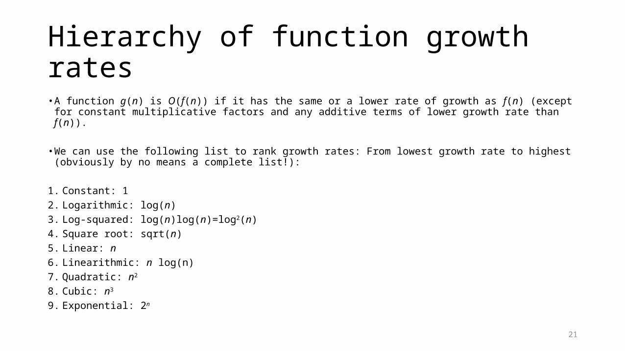
Hierarchy of function growth rates

• A function g(n) is O(f(n)) if it has the same or a lower rate of growth as f(n) (except for constant multiplicative factors and any additive terms of lower growth rate than f(n)).

• We can use the following list to rank growth rates: From lowest growth rate to highest (obviously by no means a complete list!):

1. Constant: 12. Logarithmic: log(n)

3. Log-squared: log(n)log(n)=log2(n)

4. Square root: sqrt(n)

5. Linear: n6. Linearithmic: n log(n)

7. Quadratic: n2

8. Cubic: n3

9. Exponential: 2n

22

Big-Oh: alternative definition

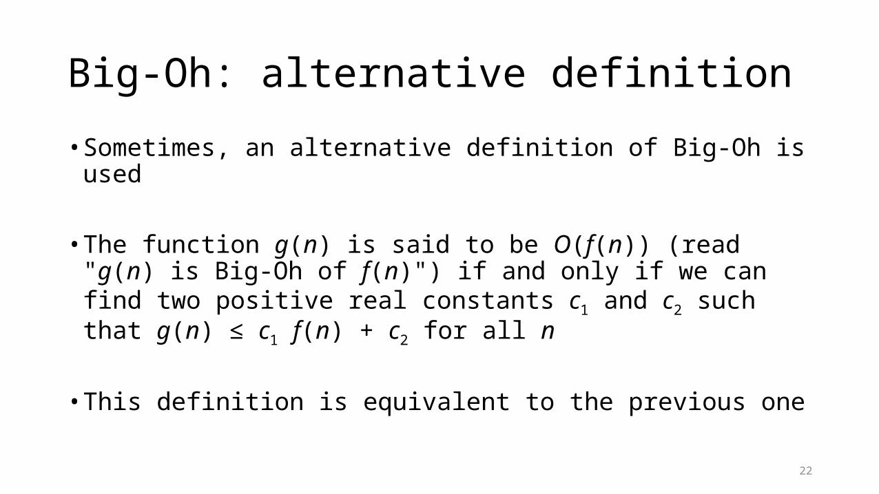
• Sometimes, an alternative definition of Big-Oh is used

• The function g(n) is said to be O(f(n)) (read "g(n) is Big-Oh of f(n)") if and only if we can find two positive real constants c1 and c2 such that g(n) ≤ c1 f(n) + c2 for all n

• This definition is equivalent to the previous one

23

“Big-Theta” notation

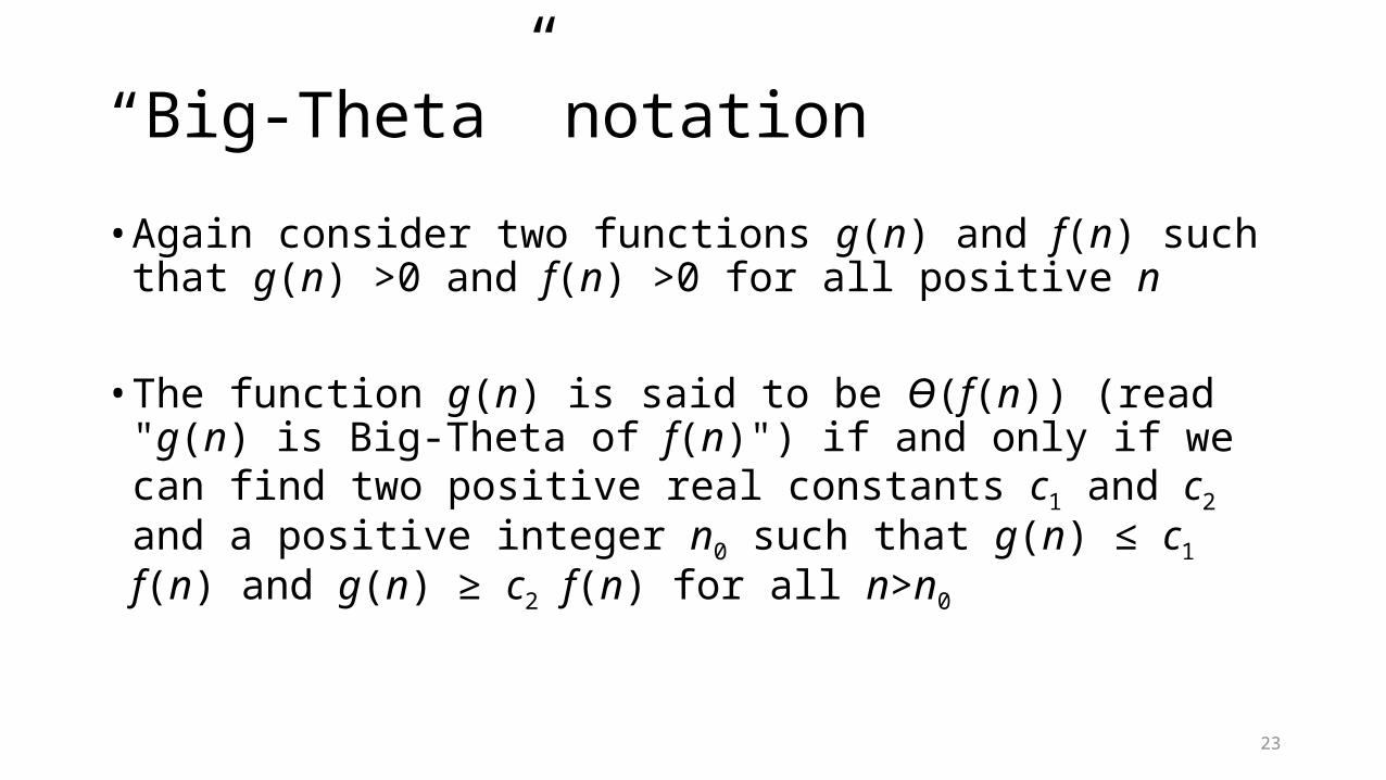
• Again consider two functions g(n) and f(n) such that g(n) >0 and f(n) >0 for all positive n

• The function g(n) is said to be ϴ(f(n)) (read "g(n) is Big-Theta of f(n)") if and only if we can find two positive real constants c1 and c2 and a positive integer n0 such that g(n) ≤ c1 f(n) and g(n) ≥ c2 f(n) for all n>n0

24

Notes on Big-Theta

• Big-Theta notation aims to capture the actual running time of an algorithm – not just the worst case scenario. It defines a class of functions that are equivalent under the Big-Theta concept

• For some algorithms, there is no Big Theta class to which they belong.

• Multiplicative constants and additive lower-order terms aside, the f(n) in Big Theta notation is unique.

• If g(n) is ϴ(f(n)), it means that g(n) has the same rate of growth as f(n) (except for the usual constant multiplicative factor and lower-order additive terms)

• If g(n) is ϴ(f(n)), then f(n) is ϴ(g(n))

25

“Big-Omega” notation

• The Big-Omega notation is the counterpart to Big-Oh: it describes a bound on the best case

• Again consider two functions g(n) and f(n) such that g(n) >0 and f(n) >0 for all positive n

• The function g(n) is said to be Ω(f(n)) (read "g(n) is Big-Omega of f(n)") if and only if we can find a positive real constant c and a positive integer n0 such that g(n) ≥ c f(n) for all n>n0

26

Notes on Big-Omega

• Big-Omega is not always unique, e.g., our original “find pairs of numbers adding up to 10” has basically the same best and worst case running time of O(n2) and Ω(n2), respectively.

• But if it is Ω(n2), it is also by implication Ω(n) .

• If a function g(n) is ϴ(f(n)), then it is by implication also O(f(n)) and Ω(f(n)).

27

Balanced search trees

• AVL trees: BST with ϴ(log n) operations in worst case, but memory hungry and computationally expensive

• Red-black trees: BST with ϴ(log n) operations

• M-ary balanced search trees

28

AVL trees

• Named after their inventors, Adelson-Velskii and Landis

• AVL trees have the property that for any node, the difference in height of the left and right subtree is at most 1

• This gives a certain amount of balance.

• Can show that the height of an AVL tree with n nodes is ϴ(log n), which ensures our operations can all be done in ϴ(log n)

• If the AVL condition is violated by an insertion or deletion, it can be restored with a type of operation called a rotation

29

AVL trees

• Our now-familiar BST tree qualifies as an AVL tree:

17

28

15

69

45

669

4

142

73

9

30

AVL trees

• This tree isn't an AVL tree:

28

69

45

669

4

142

73

9

For which node(s)is the AVL tree condition not met?

31

AVL trees

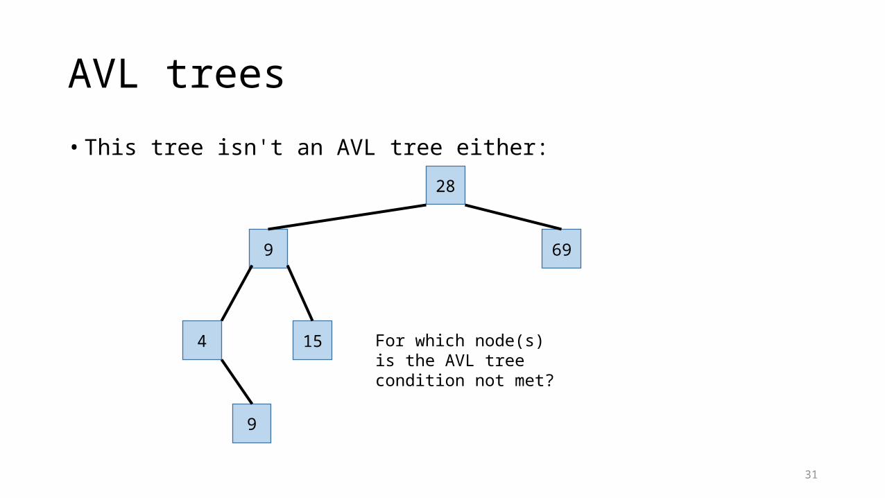
• This tree isn't an AVL tree either:

28

15

69

9

4

9

For which node(s)is the AVL tree condition not met?

32

Red-black trees

• A red-black BST assigns colours red and black to each node of the BST

• The root itself is always black

• Every child of a red node must be black

• Every path from the root to a leaf has exactly b black nodes

• This restricts the tree to a height of at most 2b and forces rebalancing before extending

• Search, insert and delete operations are all O(log n)

• Rebalancing on insert is performed by repainting of individual nodes and/or a variety of rotations similar to those in AVL trees. What exactly happens depends on the actual scenario encountered.

33

m-ary search trees

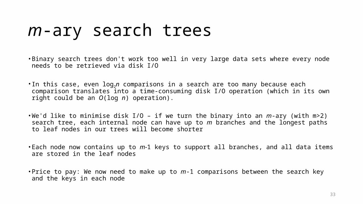
• Binary search trees don't work too well in very large data sets where every node needs to be retrieved via disk I/O

• In this case, even log2n comparisons in a search are too many because each comparison translates into a time-consuming disk I/O operation (which in its own right could be an O(log n) operation).

• We'd like to minimise disk I/O – if we turn the binary into an m-ary (with m>2) search tree, each internal node can have up to m branches and the longest paths to leaf nodes in our trees will become shorter

• Each node now contains up to m-1 keys to support all branches, and all data items are stored in the leaf nodes

• Price to pay: We now need to make up to m-1 comparisons between the search key and the keys in each node

34

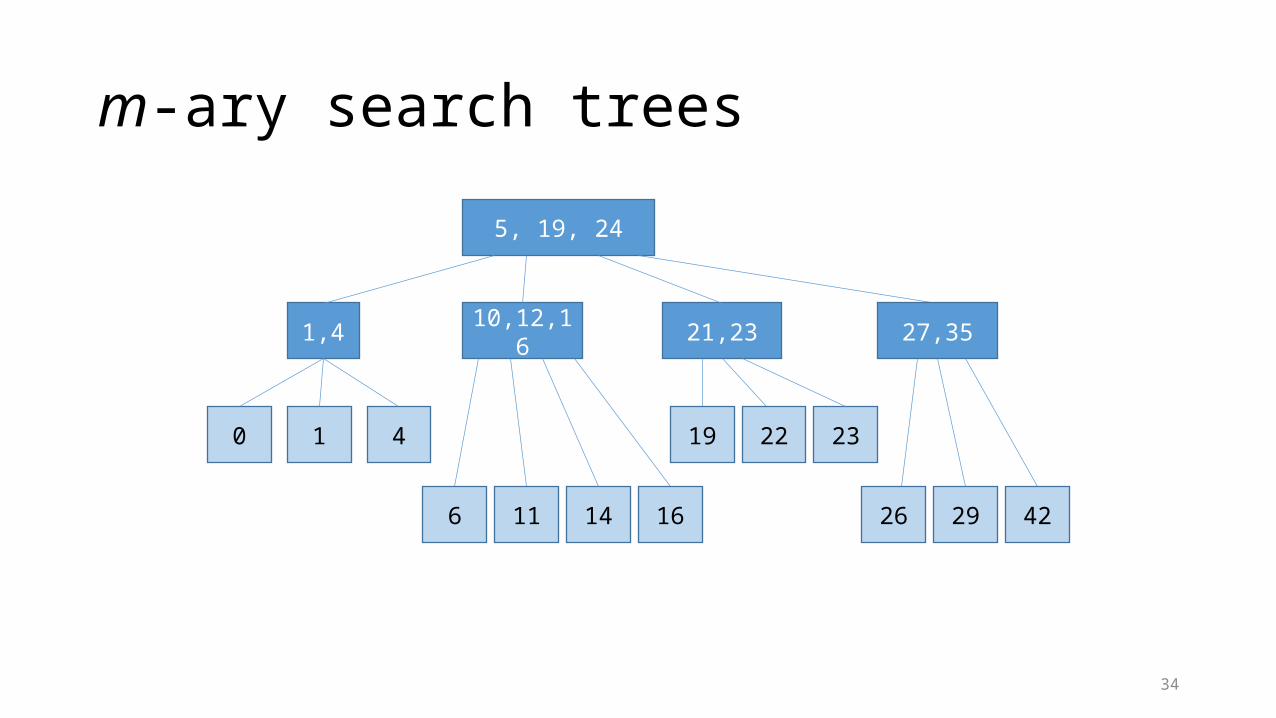
m-ary search trees

5, 19, 24

1,4

0 1 4

10,12,16

6 11 14 16

21,23

19 22 23

27,35

26 29 42

35

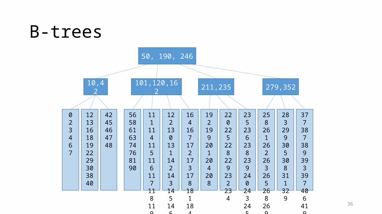
B-trees

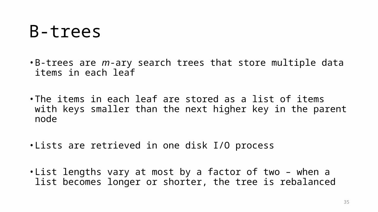
• B-trees are m-ary search trees that store multiple data items in each leaf

• The items in each leaf are stored as a list of items with keys smaller than the next higher key in the parent node

• Lists are retrieved in one disk I/O process

• List lengths vary at most by a factor of two – when a list becomes longer or shorter, the tree is rebalanced

36

B-trees50, 190, 246

10,42

023467

12131618192229303840

4245464748

101,120,162

5658616374768190

111114115116117118119

122130131142143145146147154

164167172173178181184

211,235

192199201204208

220225228229232234

235236238239240243245

279,352

258261262263265268269273276277

283299305308311329

377387389393397406419435497499