1

Compressed Sensing Microscopy with ScanningLine Probes

Han-Wen Kuo , Anna E. Dorfi , Daniel V. Esposito and John N. Wright , Member, IEEE

Abstract—In applications of scanning probe microscopy, im-ages are acquired by raster scanning a point probe across asample. Viewed from the perspective of compressed sensing(CS), this pointwise sampling scheme is inefficient, especiallywhen the target image is structured. While replacing pointmeasurements with delocalized, incoherent measurements hasthe potential to yield order-of-magnitude improvements in scantime, implementing the delocalized measurements of CS theoryis challenging. In this paper we study a partially delocalizedprobe construction, in which the point probe is replaced witha continuous line, creating a sensor which essentially acquiresline integrals of the target image. We show through simulations,rudimentary theoretical analysis, and experiments, that theseline measurements can image sparse samples far more efficientlythan traditional point measurements, provided the local featuresin the sample are enough separated. Despite this promise,practical reconstruction from line measurements poses additionaldifficulties: the measurements are partially coherent, and realmeasurements exhibit nonidealities. We show how to overcomethese limitations using natural strategies (reweighting to copewith coherence, blind calibration for nonidealities), culminatingin an end-to-end demonstration.

Index Terms—compressed sensing · scanning probe mi-croscopy · nonlocal scanning probe · tomography · sparserecovery.

I. INTRODUCTION

SCANNING probe microscopy (SPM) is a fundamentaltechnique for imaging interactions between a probe and

the sample of interest. Unlike traditional optical microscopy,the resolution achievable by SPM is not constrained by thediffraction limit, making SPM especially advantageous fornanoscale, or atomic level imaging, which has widespreadapplications in chemistry, biology and materials science [1].Conventional implementations of SPM typically adopt a rasterscanning strategy, which utilizes a probe with small and sharptip, to form a pixelated heatmap image via point-by-pointmeasurements from interactions between the probe tip andthe surface. Despite its capability of nanoscale imaging, SPMwith point measurements is inherently slow, especially whenscanning a large area or producing high-resolution images.

Manuscript received September 25, 2019. The authors would like toacknowledge funding support from the Columbia University SEAS Interdisci-plinary Research Seed (SIRS) Funding program, and NSF CDS&E 1710400.(Corresponding author: Han-Wen Kuo).

H.-W. Kuo and J. N. Wright are with Department of Electrical Engineeringand Data Science Institute, Columbia University, New York, NY, 10025. Email:hk2673@columbia.edu and jw2966@columbia.edu.

A. E. Dorfi and D. V. Esposito are with Department of Chemical Engineering,Electrochemical Energy Center and Lenfest Center for Sustainable Energy,Columbia University, New York, NY, 10025. Email: de2300@columbia.eduand aed2521@columbia.edu.

Fig. 1. Scanning electrochemical microscope with continuous line probe. Left:the lab made SECM device with line probe, mounted on an automated probearms with a rotating sample stage. Right: closeup side view of the line probenear the sample surface.

When the target signal is highly structured, compressedsensing (CS) [2], [3], [4] suggests it is possible to design adata acquisition scheme in which the number of measurementsis largely dependent on the signal complexity, instead ofthe signal size, from which the signal can be efficientlyreconstructed algorithmically. In nanoscale microscopy, imagesare often spatially sparse and structured. CS theory suggestsfor such signals, localized measurements such as pointwisesamples are inefficient. In contrast, delocalized, spatially spreadmeasurements are better suited for reconstructing a sparseimage.

Unfortunately, the dense (delocalized) sensing schemessuggested by CS theory (and used in other applications, e.g.,[5], [6], [7]) are challenging to implement in the settingsof micro/nanoscale imaging. Motivated by these concerns,[8] introduced a new type of semilocalized probe, knownas a line probe, which integrates the signal intensity alonga straight line, and studied it in the context of a particularmicroscopy modality known as scanning electrochemicalmicroscopy (SECM) [9], [10]. In SECM with line probe, theworking end of the probe consists of a straight line, whichproduces a single measurement by collecting accumulatedredox reaction current induced by the probe and sample. Theseline measurements are semilocalized, sample a spatially sparseimage more efficiently than measurements from point probes,and “have an edge” for high resolution imaging since a thinand sharp line probe can be manufactured with ease. Moreover,experiments in [8] suggest that a combination of line probes andcompressed sensing reconstruction could potentially yield order-of-magnitude reductions in imaging time for sparse samples.

Realizing the promise of line probes (both in SECM andin microscopy in general) demands a more careful studyof the mathematical and algorithmic problems of imagereconstruction from line scans. Because these measurements

arX

iv:1

909.

1234

2v1

[ee

ss.I

V]

26

Sep

2019

2

θ1θ2...θm

inputscan

angles

scanm lines

sample

lineprobe

scanpath

rotateθ2−θ1

rotateθ3−θ2

· · ·

linescans

...

inputangles,lines,basis

sparserecon-

struction

sampleimage

Microscopic Line Scans Computational Image Reconstruction

Fig. 2. Scanning procedure of SECM with continuous line electrode probe. The user begins with mounting the sample on a rotational stage of microscopeand chooses m scanning angles. The microscope then carries on sweeping the line probe across the sample, and measures the accumulated current generatedbetween the interreaction of probe and the sample at equispaced intervals of moving distance. After a sweep ends, the sample is rotated to another scanningangle and the scanning sweep procedure repeats, until all m line scans are finished. Collecting all scan lines, and providing the information of the scanningangles, the microscope system parameters (such as the point spread function) and the sparse representing basis of image, the final sample image is producedvia computation with sparse reconstruction algorithm.

are structured, they deviate significantly from conventional CStheory, and basic questions such as the number of line scansrequired for accurate reconstruction are currently unanswered.Moreover, practical reconstruction from line scans requiresmodifications to accommodate nonidealities in the sensingsystem. In this paper, we will address both of these questionsthrough rudimentary analysis and experiments, showing thatif the local features are either small or separated, then stableimage reconstruction from line scans is attainable.

In the following, we will first describe the scanning pro-cedure and introduce a mathematical model for line scans inSection II. Section III discusses several important propertiesof this measurement model, including a rudimentary study ofcompressed sensing reconstruction with line scans of a spatiallysparse image. In Section IV, we give a practical algorithmfor reconstruction from line scans, which accommodatesmeasurement nonidealities. Finally, Section V demonstratesour algorithm and theory by efficiently reconstructing bothsimulated and real SECM examples.

A. Contribution

• We expose the lowpass property of line scans, and withrudimentary analysis showing that the exact reconstructionof a sparse image is possible with only three line scansprovided these features are well-separated.

• We describe the challenges associated with image re-construction from practical line scans, due to the highcoherence of measurement model and inaccurate estimateof point-spread-function. Our reconstruction algorithmaddresses these issues.

• Based on this theory and algorithmic ideas, we demon-strate a complete algorithm for image reconstruction ofSECM with line scans, which includes an efficient algo-rithm for computation of image reconstruction, yieldingimproved results compared to [8].

B. Related work

1) Compressed sensing tomography: Line measurementsalso arise in computational tomography (CT) imaging, aclassical imaging modality (see e.g., [11], [12], [13]), withgreat variety of applications ranging from medical imaging to

material science [14], [15], [16]. Classical CT reconstructionrecovers an image from densely sampled line scans, byapproximately solving an inverse problem [17], [18]. Thesemethods do not incorporate the prior knowledge of the structureof the target image, and degrade sharply when only a few CTscans are available. Compressed sensing offers an attractivemeans of reducing the number of measurements needed foraccurate CT image reconstruction, and has been employedin applications ranging from medical imaging to (cryogenic)electron transmission microscopy [19], [20], [21], [22], [23],[24], [25], [26]. The dominant approach assumes that thetarget image is sparse in a Fourier or wavelet basis, andreconstructs it via `1 minimization or related techniques. Imagesin SECM and related modalities typically exhibit much strongerstructure: they often consist some number of small particles[27], [28], or other repeated motifs [29]. In this situation, CS isespecially promising. On the other hand, as we will see below,understanding the interaction between line scans and spatiallylocalized features demands that we move beyond conventionalCS theory.

2) Mathematical theory of line scans: Radon transformand image super-resolution: The question of recoverabilityfrom line measurements is related to the theory of the Radontransform, which corresponds to a limiting situation in whichline scans at every angle are available [30], [31], [32]. TheRadon transform is invertible, meaning perfect reconstructionis possible (albeit not stable) in this limiting situation. Dueto the projection slice theorem [33], the line projections areinherently lowpass, and so the line scan reconstruction problemis related to superresolution imaging [34]. When the imageof interest consists of sparse point sources, the image can bestably recovered from its low-frequency components, providedthe point sources are sufficiently separated [35]. Similarly, wecan hope to achieve stable recovery of localized features fromline scans as long as the features are sufficiently separated.

II. LINE SCAN MEASUREMENT MODEL

To implement line scans for SECM, a line probe (Figure 1)is mounted on an automated arm which positions the probeonto the sample surface. The line scan signal is generated byplacing this line probe in different places, and measuring theintegrated current induced by the interaction between the line

KUO et al.: COMPRESSED SENSING MICROSCOPY WITH SCANNING LINE PROBES 3

probe and the electroactive part of the sample. In a pragmaticscanning procedure (Figure 2), the user will choose distinctscanning angles θ1, . . . , θm. For each angle θ, the line probe isoriented in direction uθ = (cos θ, sin θ) and swept along thenormal direction u⊥θ = (sin θ,− cos θ). Each sweep of probegenerates the projection of the target image along the probedirection uθ; collecting these projections for each θi, we obtainour complete set of measurements.

A. Line projection

To describe the scanning procedure more precisely, we beginwith a mathematical idealization, in which the probe measuresa line integral of the image. In this model, when the probebody is oriented in direction uθ at position t, we observe theintegral of the image over `θ,t := w ∈ R2

∣∣ 〈u⊥θ , w〉 = t:

Lθ[Y ](t) :=∫`θ,tY (w) dw

=∫sY(s · uθ + t · u⊥θ

)ds. (II.1)

Collecting these measurements for all t, we obtain a functionLθ[Y ] which is the projection of the image along the directionuθ. We refer to the operation Lθ : L2(R2) → L2(R) as aline projection. Combining projections in m directions Θ =θimi=1, we obtain an operator LΘ : L2(R2)→ L2(R× [m]):

LΘ[Y ] := 1√m

[Lθ1 [Y ], . . . ,Lθm [Y ] ] . (II.2)

B. Line scans

In reality, it is not possible to fabricate an infinitely sharpline probe, and hence our measurements do not correspondto ideal line projections. The line probe has a response in itsnormal direction, causing a blurring effect that can be modeledas convolution with point spread function ψ along the sweepingdirection. In SECM, ψ is typically skewed with a long tail inthe sweeping direction. Accounting for this effect is importantfor obtaining accurate reconstructions in practice. In this morerealistic model, our measurements R ∈ L2(R× [m]) become

R = 1√m

[ψ ∗ Lθ1 [Y ] , . . . ,ψ ∗ Lθm [Y ]]

=: ψ ∗ LΘ [Y ] . (II.3)

This measurement consists of m functions ψ ∗Lθi [Y ] (t) of asingle (real) variable t, which corresponds to the translation ofthe probe in the u⊥θi direction. In practice, we do not measurethis function at every t, but rather collect n equispaced samples.Write the sampling operator as S : L2[R] → Rn, then ourdiscretized measurements Ri with scanning angle θi is definedas Ri = SRi. Collect all m discrete line scans, the finalmeasurement R ∈ Rn×m is written as

R = [SR1, . . . ,SRm] =: SR. (II.4)

Our task is to understand when and how we can reconstructthe target image Y from these samples.

Rθ(t)

t

θ (sin θ,− cos θ)

`θ,t

wi

Y

Fig. 3. Mathematical expression of a single measurement from the line probe.When the stage rotate by θ clockwise, the relative rotation of probe to sampleis counterclockwise by θ. The grey line in the figure represents the rotatedline probe, orienting in direction uθ = (cos θ, sin θ), and is sweeping indirection u⊥θ = (sin θ,− cos θ). When it comes across the point wi wheret = 〈u⊥θ , wi〉, it integrates over the contact region `θ,t between the probeand substate and produces a measurement Rθ(t).

III. PROMISES AND PROBLEMS OF LINE SCANS

The line measurements Lθ enjoy two major advantages asan imaging model: (i) compared to pointwise measurements,the line projections are more delocalized, hence can be moreefficient while measuring a spatially sparse signal; and (ii) itis easier to build a sharp edge for the line probe (even sharperthen the tip diameter of a point probe), which is well-suited todetect ultra-high frequency components in the probe sweepingdirection. This makes possible fast and high resolution imagingfor scanning microscopes.

Nevertheless, the line projection comes with a few apparentdisadvantages. Consider a limiting scenario, in which infinitelymany line projections are available, corresponding to everyangle in [0, 2π). The projection slice theorem implies thatthese measurements are invertible, and the image can beperfectly reconstructed. However, this reconstruction is notstable: viewed in Fourier domain, these measurements areapproximately lowpass, and inverting them amplifies highfrequencies. This that means even though a single line pro-jection can be highly sensitive to directional high frequencycomponents, the cumulative line projections are not. Stablyinverting them requires prior knowledge of the image to bereconstructed. Moreover, to reconstruct an image consistingof multiple localized features, these features need to be eithersufficiently separated.

The other disadvantage of line projections can be viewedfrom the CS perspective, that the line scans measurementsmodel are not coherent—even if the local features are wellseparated. This means that in practice, when using only a fewline scans for reconstruction, the number of lines required forexact reconstruction cannot be obtained from conventional CStheory. More importantly, the coherence of line projections cancause issues in image reconstruction; conventional methodstend to produce reconstructions with incorrect magnitudes.

Finally, we discuss measurement nonidealities due to vari-ability in the PSF ψ. In the next section, we will provide an

4

algorithmic solution addressing both issues from the coherenceof line projections and incomplete information of PSF.

A. CS of line projections for highly localized image

Compressed sensing, in its simplest form, asserts that ifthe target signal has sparse representation, it can be exactlyreconstructed from a few measurements, provided those mea-surements are incoherent to the basis of sparsity. Since inmicroscopic imaging the underlying signal is often structuredand spatially localized, CS theory suggests that delocalizedmeasurements, such as line projections, could yield moreefficient reconstructions than conventional point measurements.

Inspired by CS, we start from providing the sufficient con-ditions of sparse image reconstruction from line measurementsvia total variation minimization [36]. Later, base on theseconditions, we demonstrate the the use of line probes can beindeed more efficient than using point probes.

Proposition III.1. [Certificate of TV-norm minimization] LetX0 =

∑w∈W αwδw

1 with |W| <∞. Given continuous com-pactly supported circular symmetric D ∈ L2(R2), scanningangles Θ = θ1, . . . , θm and measurement R = LΘ[D ∗X0].Suppose there exists Q as finite sum of weighed Diracs suchthat

D ∗ L∗Θ[Q](w) = sign (αw) , w ∈ W∣∣∣D ∗ L∗Θ[Q](w)

∣∣∣ < 1, w 6∈ W.(III.1)

If the Gram matrix G ∈ R|W|×|W|, defined as

Gij =⟨LΘ[D ∗ δwi ], LΘ[D ∗ δwj ]

⟩, wi,wj ∈ W (III.2)

is positive definite, then X0 is the unique optimal solution to

minX∈BV(R2)

∫w|X| (dw) s.t. R = LΘ[D ∗X].

(III.3)

Proof. First we show the existence result. Note that X0

satisfies the equalitiy constraint (III.3) automatically, and sincetotal variation of Dirac measure is exactly one,∫

|X0| (dw′) =∑w

∫|αw| δw(dw′) =

∑w |αw|

=∑w αw ·D ∗ L∗Θ

[Q](w)

then sinceD is circular symmetric,D∗L∗Θ[Q](w) = 〈δw,D∗

L∗Θ[Q]〉 = 〈LΘ [D ∗ δw] , Q〉, we derive∫

|X0| (dw′) = 〈LΘ [D ∗∑w αwδw] , Q〉 = 〈R, Q〉

which certifies that X0 is an optimal solution to the problemsince the duality gap

∫|X0| (dw′) − 〈R, Q〉 = 0. For

uniqueness, let X ′ =∑w′∈W′ α

′w′δw′ to be another optimal

solution with W ′ 6⊆ W , since we know X ′ is primal feasibleR = LΘ [D ∗X ′], then∫

|X0| (dw′) = 〈R, Q〉 = 〈LΘ [D ∗X ′] , Q〉= 〈X ′,D ∗ L∗Θ[Q]〉

1The Dirac measure δ satisfies∫D(w)δwi (dw) =D(wi) for continuous

and compactly supported D and has total variation∫|δwi | (dw) = 1, so

D ∗ δw represents D with center at w [37]. As a functional, we write〈δwi , ·〉 : L2(R2)→ R where 〈δwi ,D〉 =D(wi).

=∑w′∈W′ α

′w′D ∗ L∗Θ

[Q](w′)

and by knowing W ′ 6⊆ W and using the second condition in(III.1):∫

|X0| (dw′) <∑w′∈W′ |α′w′ | =

∫|X ′| (dw′)

thus X ′ is an optimal solution only if W ′ ⊆ W . Finallyuniqueness of X0 follows from injectivity of LΘ[D ∗ · ] overW from (III.2).

Specifically, when the target image is highly spatially sparseand its components are well separated, the line projections canbe a very efficient measurement model. A concrete exampleis demonstrated in Lemma III.2, where we assume the sparsecomponent of the image signal are small and separated discs;if the radius of the discs are sufficiently small, then, perhapssurprisingly, only three line projections is required to exactlyreconstruct the image via efficient algorithm.

Lemma III.2. [Reconstruction from three line projection]Consider an image consists of k ≥ 2 discs radius r. Ifthe centers w1, . . .wk are at least separated by 2

C k2r, then

three continuous line projections with probe direction chosenindependent uniformly at random suffice to recover the imagewith probability at least 1− C via solving (III.3).

Proof. We first argue that with high probability, no pair ofdiscs overlaps within any line scan. Let θi ∼i.i.d. Unif[−π, π)denote the i-th scanning angle. Write d as the minimum distancebetween all pairs of (wi,wj), the probability that any particularpair of two discs overlap is bounded as

P[Two discs overlap on line scan Ri

]≤ P

[θi ∈

[− sin−1

(2rd

), sin−1

(2rd

)]]= 2

π sin−1 2rd (III.4)

Using the assumption that R < d8 to bound sin−1( 2r

d ) < 2πr3d

and summing the failure probability over all three line scansand k(k−1)

2 pairs of discs, we obtain:

P[Two of the k discs overlap at either R1, R2, R3

]≤ 3k2

2 · P[Two discs overlap on line scan R1

]≤ 3k2

π sin−1(

2rd

)≤ 2k2r

d

≤ C (III.5)

Thus, with probability at least 1−C, no pair of discs overlapsin any line scan.

Since there are no overlapping discs in any line, a singleline projection Ri(t) with scan angle θi has largest magnitudeat points t where the probe body passes the disc center wj .These points of largest magnitude βj is located at 〈u⊥θi ,wj〉on Ri, or equivalently,

Lθi [D ∗ δwj ](〈u⊥θi ,wj〉) = βj , i = 1, 2, 3 (III.6)

Using these points, we construct the dual certificate Qi forangle θi, where

Qi =∑kj=1

1√3βjδ〈u⊥θi ,wj〉

(III.7)

KUO et al.: COMPRESSED SENSING MICROSCOPY WITH SCANNING LINE PROBES 5

and Q =[Q1, Q2, Q3

]. Using this certificate we verify (III.1)

holds. For the equality, calculate at every wj ∈ w1, . . .wk:

D ∗ L∗θ1,θ2,θ3[Q](wj)

= 〈D ∗ L∗θ1,θ2,θ3[Q], δwj 〉 = 1√

3

∑3i=1〈Qi,Lθi [D ∗ δwj ]〉

= 1√3

∑3i=1

⟨1√3βjδ〈u⊥θi ,wj〉

,Lθi [D ∗ δwj ]⟩

= 13βj

∑3i=1 Lθi [D ∗ δwj ](〈u⊥θi ,wj〉) = 1 (III.8)

where the third line is by plugging in Q and derived with nooverlap property; the forth line via plugging in (III.6). For theinequality, calculate∣∣∣D ∗ L∗θ1,θ2,θ3[Q](w)

∣∣∣=∣∣∣∑3

i=1

∑kj=1

13βjLθi [D ∗ δw](〈u⊥θi ,wj〉)

∣∣∣ (III.9)

which is derived similarly as (III.8). Now, by observing Lθ[D∗δw] has unique local maximum at 〈u⊥θ ,w〉, each summand(w.r.t. i) in (III.9) is strictly less than 1 if w does not satisfy

∃ j ∈ 1, . . . , k , 〈u⊥θi , w〉 = 〈u⊥θi , wj〉. (III.10)

Accordingly, define the back projection line set `θi,tj as

`θi,tj := w ∈ R2∣∣ 〈u⊥θi , w〉 = 〈u⊥θi , wj〉, (III.11)

we want to show that for every w 6∈ w1, . . . ,wk,

w 6∈ ∩3i=1

(∪kj=1 `θi,tj

)(III.12)

then (III.9) is strictly less then 1.W.l.o.g., write wj` = `θ1,tj ∩ `θ2,t` . Suppose the point wj`

is in the third line set ∪kj=1`θ3,tj , then there exists some disccenter wq such that 〈u⊥θ3 , wj`〉 = 〈u⊥θ3 , wq〉. Since θ3 isgenerated uniform randomly, we conclude that for any j, `:

P[∃ q ∈ 1, . . . , k s.t. wj` ∈ `θ3,tq

]= 0. (III.13)

The direction uθ3 is not aligned with the line formed bywj`,wq almost surely. This proves (III.12).

Finally, the diagonal entries of Gram matrix G defined in(III.2) is strictly positive, and the off-diagonal entries Gij canbe derived as

Gij = 13

∑3t=1

⟨Lθt [D] ∗ δwi ,Lθt [D] ∗ δwj

⟩= 0 (III.14)

by no overlap property. Hence G is positive definite. Thisconcludes that solving total variation minimization successfullyreconstruct the image from three line projections.

The proof idea can be depicted pictorially in Figure 4, inwhich we show the construction of dual certificate Q, and theback projection operation L∗Θ on Q which we used in the proofto certify the optimality. In fact, as we will show later, theoperation L∗Θ is the cornerstone for most of the reconstructionalgorithms in computed tomography, as well as in our sparsereconstruction algorithm.

∪kj=1`θ1,tj

R1

∪kj=

1θ 2,t j

R2

∪kj=

1 `θ3,tj

R3

w1

wk

Fig. 4. Proof sketch for sufficiency of image recovery from three lineprojections. Given a sample with separated tiny discs w1, . . .wk (blackdots), randomly choosing three lines projection forms lines R1, R2, R3, inwhich all the discs after line projection (red dots) are well-separated. Fromeach of these lines, we construct the dual Q as center of red dots, and aback projection image form the dual (dash lines), forming the set ∪kj=1`θi,tj .Intersection of three such line sets is exactly the set of ground truth disccenters.

B. Reconstructability from line projections of localized imagein practice

While the microscopic images are often sparse in the spatialdomain, they rarely satisfy the conditions of Lemma III.2, inwhich the local features are uncharacteristically small and farapart. In the following, we will show in practical applicationof line scans, when the image consists of multiple localizedmotifs, the performance of line measurements degrades oncethe ratio between the size of motifs and its separating distanceincreases.

1) Coherence of line projection of two localized motif: Westart from a simple case considering an image with two motifslocated at different locations. Define a 2 × 2 Gram matrixG with its ij-th entries being coherence [38] between lineprojected signal of two motifs D with center at wi and wjrespectively,

Gij =⟨LΘ[D ∗ δwi ], LΘ[D ∗ δwj ]

⟩. (III.15)

If the off-diagonal entry Gij is small in magnitude comparedto the diagonal entries Gii,Gjj , then it suffices to reconstructthe image exactly with efficient algorithm. Conversely, if G isill-conditioned or even rank-deficient, then exact recovery willbe impossible.

Lemma III.3. [Coherence of line projection Gaussians] LetD be the two-dimensional Gaussian functions with covariancerI2 and normalized in a sense that ‖L0[D]‖L2 = 1. If θis uniformly random, then the expectation of inner productbetween two line projected D at different locations wi,wj isbounded by(

1− d2

8r2

)1d≤2r + r

2d1d>2r

≤ Eθ⟨Lθ[D ∗ δwi ], Lθ[D ∗ δwj ]

⟩≤ 1√

1+d2/4r2. (III.16)

where d = ‖wi −wj‖2.

6

Proof. Write d(t) = L0

[D](t), where d is a one-dimensional

standard Gaussian with deviation r. Since D is circularsymmetric, the line projection of D in any angle is identical,that is, Lθ[D] = L0[D] for every θ. Also write wi −wj =d(cosφ, sinφ), then⟨

Lθ[D ∗ δwi ], Lθ[D ∗ δwj ]⟩

=⟨Lθ[D] ∗ Lθ[δwi ], Lθ[D] ∗ Lθ[δwj ]

⟩=⟨d ∗ d, δ|u∗θ(wi−wj)|

⟩= (d ∗ d) (d cos(θ − φ))

= exp(−d2 cos2(θ−φ)

4r2

), (III.17)

where the first equality is by interchanging iterated integrals;the second equality is by knowing the adjoint of convolutionis correlation and d is symmetric; and the final equality is byobserving that d ∗ d is a Gaussian function with variance

√2r

and (d ∗ d)(0) = 1.We derive the expectation upper bound of (III.17) over θ as

Eθ⟨Lθ[D ∗ δwi ], Lθ[D ∗ δwj ]

⟩= 1

π

∫ π0

exp(−d2 cos2 θ)/4r2

)dθ

≤ 1π

∫ π0

11+(d2 cos2 θ)/4r2 dθ

= 1√1+d2/4r2

(III.18)

by utilizing exp(−x2)(1 + x2) < 1 in the second inequality.As for the lower bound of (III.17), from its first equality,

we calculate when d > 2r, then

1π

∫ π0

exp(− (d2 cos2 θ)/4r2

)dθ

≥ 1π

∫ π0

exp(−(d2/4r2) · (2r2/d2)

)· 1cos2 θ≤2r2/d2 dθ

≥ 2π · exp

(− 1

2

)·(π2 − cos−1

√2r2/d2

)≥ 2

π · exp(− 1

2

)· (√

2r/d)

≥ r/2d. (III.19)

using cos−1 x ≤ π2 −x for x ∈ [0, 0.5]. And when d ≤ 2r, we

simply have

1π

∫ π0

exp(− (d2 cos2 θ)/4r2

)dθ ≥ 1− d2/8r2 (III.20)

via Taylor expansion at d/2r = 0

Lemma III.3 shows the coherence between line projectionsof two bell-shaped motif with radius ≈r and center distance dis dominated by the distance-to-diameter ratio d/2r. Because ofthe projection slice theorem, the matrix EθG is always positivedefinitive. However, its condition number greatly increaseswhen the image consists of highly overlapping local features.When the ratio is small, say d/2r < 1, in which the twoprojected motifs are overlapping, then EθGij will be closeto one as with the diagonals, implies EθG become severelyill-conditioned even in the two-sparse case. Generally speaking,line scans are not CS-theoretical optimal sampling method forrecovering images consisting of superposing discs.

20 × 20 × 1.15 motifs

d/2r = 2

12 102 202 3020

.5

1

number of motifs

λmin(G)

d/2r = 0.5 d/2r = 1.0d/2r = 1.5 d/2r = 2.0d/2r = 2.5 d/2r = 3.0d/2r = 3.5 d/2r = 4.0

× 1.15

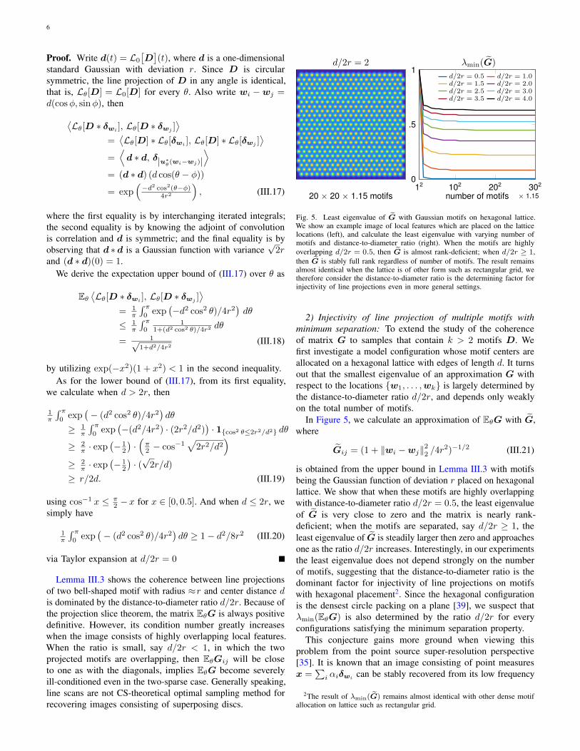
Fig. 5. Least eigenvalue of G with Gaussian motifs on hexagonal lattice.We show an example image of local features which are placed on the latticelocations (left), and calculate the least eigenvalue with varying number ofmotifs and distance-to-diameter ratio (right). When the motifs are highlyoverlapping d/2r = 0.5, then G is almost rank-deficient; when d/2r ≥ 1,then G is stably full rank regardless of number of motifs. The result remainsalmost identical when the lattice is of other form such as rectangular grid, wetherefore consider the distance-to-diameter ratio is the determining factor forinjectivity of line projections even in more general settings.

2) Injectivity of line projection of multiple motifs withminimum separation: To extend the study of the coherenceof matrix G to samples that contain k > 2 motifs D. Wefirst investigate a model configuration whose motif centers areallocated on a hexagonal lattice with edges of length d. It turnsout that the smallest eigenvalue of an approximation G withrespect to the locations w1, . . . ,wk is largely determined bythe distance-to-diameter ratio d/2r, and depends only weaklyon the total number of motifs.

In Figure 5, we calculate an approximation of EθG with G,where

Gij = (1 + ‖wi −wj‖22 /4r2)−1/2 (III.21)

is obtained from the upper bound in Lemma III.3 with motifsbeing the Gaussian function of deviation r placed on hexagonallattice. We show that when these motifs are highly overlappingwith distance-to-diameter ratio d/2r = 0.5, the least eigenvalueof G is very close to zero and the matrix is nearly rank-deficient; when the motifs are separated, say d/2r ≥ 1, theleast eigenvalue of G is steadily larger then zero and approachesone as the ratio d/2r increases. Interestingly, in our experimentsthe least eigenvalue does not depend strongly on the numberof motifs, suggesting that the distance-to-diameter ratio is thedominant factor for injectivity of line projections on motifswith hexagonal placement2. Since the hexagonal configurationis the densest circle packing on a plane [39], we suspect thatλmin(EθG) is also determined by the ratio d/2r for everyconfigurations satisfying the minimum separation property.

This conjecture gains more ground when viewing thisproblem from the point source super-resolution perspective[35]. It is known that an image consisting of point measuresx =

∑i αiδwi can be stably recovered from its low frequency

2The result of λmin(G) remains almost identical with other dense motifallocation on lattice such as rectangular grid.

KUO et al.: COMPRESSED SENSING MICROSCOPY WITH SCANNING LINE PROBES 7

information (with frequency cutoff fc) whenever the pointsources have minimum separation d > C/fc for some constantC, regardless of the number of such point measures in x. Inour scenario, we will show that the expected line projectionEθL∗θLθ is also a low-pass filter; and since the local featuresD is also often consists of low frequency components, ourline projections LΘ[D ∗X] can be modeled as the low-passmeasurements from sparse mapX , implying stable and efficientsparse reconstruction is possible as long as X is enoughseparated under infinitely many line measurements of all angles.

Lemma III.4. [Lowpass property of line projections] SupposeD is two-dimensional Gaussian of covariance r2I with‖L0[D]‖L2 = 1 and X is finite summation of Dirac measure.If θ is uniformly random, then EθD ∗ L∗θLθ[D ∗ X] is alow-pass filter K on X with cut-off frequency fc satisfies

fc = 1r ·min

2r2ε−1,

√|log (8r2ε−1)|+ 0.2

(III.22)

in a sense that max‖ξ‖2≥fc |F2 K (ξ)| ≤ ε.

Proof. We start with restating projection slice theorem asF1Lθ[Y ] = Sθ[F2Y ], where F1, F2 are unitary Fouriertransform in one, two-dimensional Euclidean space respectively,Sθ is the slice operator defined as Sθ[Y ](r) = Y (ru⊥θ ) [33].

Notice that Y = D ∗X ∈ L1∩L2(R2) therefore its Fouriertransform is well defined, we expand L∗θLθ in Fourier domainwith slice operator Sθ, write Y = F2Y . and derive

EθL∗θLθ[Y ](w)

= EθF∗2S∗θF−1∗1 F−1

1 SθF2Y (w)

= Eθ∫ξ∈R2 exp (j2π 〈ξ,w〉) · S∗θ [Sθ[Y ]](ξ) dξ

= Eθ∫t∈R Sθ[exp (j2π 〈·,w〉)](t) · Sθ[Y ](t) dt

= 12π

∫ 2π

θ=0

∫t∈R exp(j2πt

⟨u⊥θ ,w

⟩) · Y (tu⊥θ ) dt dθ

= 22π

∫ 2π

θ=0

∫t≥0

exp(j2πt⟨u⊥θ ,w

⟩) · Y (tu⊥θ ) dt dθ

=∫ξ∈R2 exp(j2πt 〈ξ,w〉) ·

(1

π‖ξ‖2

)· Y (ξ) dξ

=(F−1

2

1

π‖ξ‖2

∗ Y

)(w), (III.23)

where the third equality is derived from definition of adjointoperator, sixth equality is by coordinate transformation frompolar to Cartesian, and the last equality is by convolution the-orem. Hence we conclude that EθL∗θLθ[Y ] is the convolutionbetween Y and a lowpass kernel with spectrum decay rate‖ξ‖−1

2 .When ‖L0[D]‖L2 = 1 and is a Gaussian function with devi-

ation r, then D(w) =

√2r√π

2πr2 exp(−‖w‖

22

2r2

)with Fourier do-

main expression as F2 D (ξ) =√

2r√π exp(−2π2r2 ‖ξ‖22).

Combine with (III.23), the spectrum of EθD ∗ L∗θLθ[D ∗ · ]becomes

F2EθD ∗ L∗θLθ[D ∗X](ξ)

= 2r√π‖ξ‖2

exp(−4π2r2 ‖ξ‖22) · F2 X (ξ).

= F2 K (ξ) · F2 X (ξ) (III.24)

-10 0 100

imax

distance/mm

curr

ent/m

A

Estimated PSF Simulated PSF

θCLP = 65

θCLP = 45

Fig. 6. The point spread function of line probe. The PSF of line probe isskewed in the probe sweeping direction. We show an estimated PSF with closeform used for reconstruction (left); and the software (LabVIEW) simulatedPSF whose shape and intensity changes as the contacting angle varies (right).

Plug in (III.22), when ‖ξ‖2 ≥ 2rε then clearly

|F2 K (ξ)| ≤ ε. Lastly for the other lower bound ‖ξ‖2 ≥1r

(√|log(8r2ε−1)|+ 0.2

), we calculate

|F2 K (ξ)| ≤ 2r2

0.2√π· exp

(−4π2

∣∣log(8r2ε−1)∣∣)

≤ 2r2

0.2√π· 1

8r2ε−1 ≤ ε. (III.25)

Remark III.5. When radius of motif is sufficiently large, thenthe cut-off frequency fc is dominated by the cut-off frequencyof motif, roughly C/r, and is sufficient to recover its locationsas long as the separation d satisfies d > C ′r (reflects theobservation of Figure 5). In cases with small (pointy) D,the cut-off frequency is mainly determined by the low-passproperty of line projection, which requires minimum separationd > Cε/r for exact reconstruction.

Finally, base on [35], when the separation condition isensured, the image of separated discs can be recovered frominfinitely many line projections via total variation minimization(or `1 when X0 on discrete grid), regardless of number ofdiscs.

C. Obstacles of image reconstruction from line scans

Besides the apparent nonideality of coherence of line scanmeasurements which is not CS theoretical optimal, this specificsampling method and its corresponding hardware limitationscauses other practical nuisances during image reconstruction.

a) High coherence of line scans: To show the coherenceis a cause for concern, we rewrite the linear operator LΘ[D∗ · ]as A, and consider the nonnegative Lasso

minX≥0

λ ‖X‖1 + 12 ‖A[X]−R‖22 (III.26)

using the observed signal R = A[X0] and linear, columnnormalized and coherent sampling method A. Denote Ω as thesupport set of solution of (III.26), write AΩ as the submatrixof A restricted on columns of support Ω, the unique solution

8

X of program (III.26) (provided if AΩ is injective) can bewritten as

Xij =[X0ij − λ(A∗ΩAΩ)−11

]+

wij ∈ Ω

Xij = 0 wij 6∈ Ω.(III.27)

When A is coherent, columns of A have large inner product,implies many entries of the matrix A∗ΩAΩ have large, positiveoff-diagonal entries close to its diagonals. When the sparsepenalty λ is large in (III.26), its solution will have incorrectrelative magnitudes since A∗ΩAΩ is not close to identity matrixas conventional CS measurements [40]. When λ is small,the solution of program will be highly sensitive to noise,occasionally lead to incorrect results.

b) Incomplete information of PSF of line scans: Anotherlayer of complexity for line probe scans is the difficulty tocorrectly identify its PSF due to hardware limitations, especiallywhen operating line scans in nanoscale. For instance in Figure 6,we show if the contacting angle between the probe and thesample varies, the corresponding PSF changes drastically inboth the peak magnitude and the shape. It turns out thateven with seemingly small changes of probe condition, thecorresponding PSF can be inevitably variated.

IV. RECONSTRUCTION FROM LINE SCANS

In this section, we introduce an algorithm for reconstructingSECM images from line scans. In all following experiments,we consider a representative class of images Y character-ized by superposing reactive species D at locations W =w1, . . . ,w|W|

⊂ R2 with intensities

α1, . . . , α|W|

⊂ R+.

Define the activation map X0 as sum of Dirac measure at W ,then Y can simply be written as convolution between D andX0:

Y = D ∗X0 =∑|W|j=1 αjD ∗ δwj . (IV.1)

The imaging reconstruction problem then can be cast as findingthe best fitting sparse map X from line scans R = SΨ ∗LΘ[Y ], and the reconstructed image is simplyD∗X . Since allassociated operations on X0 (convolution with D,ψ and lineprojection LΘ) are all linear, this becomes a sparse estimationproblem, which can be solved via the Lasso. In practice, duethe resolution limit of probe and the sampling operation S , wedo not aiming to find exact X in a continuous space. Instead,we will solve the discretized version of this sparse recoveryproblem, which assume X resides on a grid. As such, theassociated Lasso problem can be written as:

minX≥0

λ∑ijXij + 1

2 ‖R− SΨ ∗ LΘ[D ∗X]‖22 . (IV.2)

A. Sparse recovery with Lasso from line projections

In light of Section III-B, the measurement performanceusing infinitely many line scans is almost dependent only onthe distance-to-diameter ratio of the local features. Since inpractice, only finite number line scan is available, we want tostudy how many line scans will be sufficient for efficient andexact sparse image reconstruction. We do this by studying theperformance of algorithm (IV.2) while assuming the line scanare idealized where the PSF is ideally all-pass in the sensethat ψ = δ.

16 64 112 160140500

3.6k

point probeline probe

20 40 60 80 100 120

140400

790

2.4k point probeline probe

16 64 112 160

3

7

11

15

1921 ≈ 50% recover

20 40 60 80 100 120

5

7

9

11

13

15 ≈ 50% recover

Fixed image size

Fixed image density

number of discs number of discs

num

bero

flin

es

num

bero

flin

es

number of discs number of discsnu

mbe

rofs

ampl

es

num

bero

fsam

ples

Fig. 7. Phase transition [8] of fixed image size (top) and fixed density (bot)on support recovery with Lasso. In each experiments, d/2r ≥ 1 is ensured. Ineither cases, the phase transitions (left) show the number of samples required isalmost linearly proportional to the number of discs for exact reconstruction. Andthe the advancement of scanning efficiency (right) is presented in comparisonwith the point probe scans. For the fixed size case, we let (image area)/(discarea) ≈ 1200; for the fixed density case, we let density ≈ (1/6)·(max density).

Figure 7 shows the reconstruction performance from linescans with varying number of lines used and number of discsin the target image Y . Each image Y is generated by randomlypopulating the discs of size r while satisfying d/2r ≥ 1 viarejection sampling, and the scan angles are also uniformlyrandom chosen. Here, two experiment settings are presented.The first is assumed that the imaging area of line scan isfixed (so the density increases linearly with more discs) andthe second is considering the cases where the density is aconstant (so the imaging area is proportional to the discamount). In the phase transition (PT) image (Figure 7, left),each pixel represents the average of 50 experiments; and ineach experiment, given random image Y and its line scansof randomly chosen angles, if solving (IV.2) correctly identifythe support map of Y , then the algorithm succeeds, and viceversa. It shows clear transition lines in both PT images, andthe comparison of scanning time between line/point probesshows clear improvement of scanning efficiency.

Interestingly if we compare the result with CS theory, whichasserts the number measurement of samples required is closeto linear proportional to signal sparsity; here, though the linescans are not CS-optimal, both PT images exhibits similarphenomenon. When the image size is fixed (up), total numberof samples m is proportional to the line count N , with PTtransition line showing linear proportionality between numberof line scans and discs N ∝ k, gives m ∝ k; on the otherhand, when the image density is fixed, the number of samples

KUO et al.: COMPRESSED SENSING MICROSCOPY WITH SCANNING LINE PROBES 9

m is proportional to N ×√k3 while the transition line in

PT is showing N ∝√k, again suggests linear proportionality

between the number of measurements and sparsity would bem ∝ N

√k ∝ k. To wrap up, these experimental results hinted

that if minimum separation of discs are ensured, then to ensureexact signal reconstruction with efficient algorithm, the numberof samples required is approximately linearly proportional tothe sparsity of image.

Finally, to formally elucidate the sample time reduction frompoint probe to line scans, we compare the consumed scanningtime using different probes in both settings under specificscenarios. (Figure 7, right). In the fixed area experiment welet the image area be 3×3 mm2 and the disc radius and theimage resolution are both 50µm (image area/disc area ratioaround 1200); for the fixed density we let all experiments haveequal density 20 discs/mm2 (nearly 1/6 of maximum densityin separating case) with same resolution. Both of the resultsshow clear improvement of scanning efficiency, with reductionof scanning time by 3 to 10 times under these signal settings.

In either case, line measurements are substantially moreefficient than measurements with a point probe. Realizing thisgain in practice requires us to modify the Lasso to cope withthe following nonidealities: (i) line scans are coherent, (ii)the PSF ψ is typically only partially known, and (iii) naiveapproaches to computing with line scans are inefficient whenthe target resolution is large. Below, we show how to addressthese issues, and give a complete reconstruction algorithm.

B. Computation of line projection

1) Fast computation of discrete line projection: The lineprojection of an image Y in direction of angle θ is equivalentto the line projection at 0 of clockwise rotated Y by angle θ.This enables an efficient line projection computationally viafast image rotation with shear transform in Fourier domain[41].

The clockwise rotation of image Y by angle θ is

Rotθ [Y ] (x, y) = Y

([cos θ − sin θsin θ cos θ

] [xy

])(IV.3)

where the rotational matrix can be decomposed into three sheartransforms[

cos θ − sin θsin θ cos θ

]=

[1 0

tan θ2 1

] [1 − sin θ0 1

] [1 0

tan θ2 1

];

write both x, y-shear transforms as

Shr-xs[Y ](x, y) = Y (x+ sy, y),

Shr-yt[Y ](x, y) = Y (x, y + tx),

then

Rotθ[Y ] = Shr-ytan

θ2

Shr-x− sin θ Shr-ytan

θ2

[Y ] .

(IV.4)

Each of the shear transform can be efficiently computed inFourier domain. Define

Sx,t(u, y) = ej2πtyu, Sy,t(x, v) = ej2πtxv, (IV.5)

3With fixed density, imaging area is proportional to disc count, and thenumber of samples is (line count)×

√(imaging area) = N ×

√k.

and Fx, Fy as n-DFT in x,y-domain, where

FxY (u, y) =∑x Y (x, y)e−j2πxu, (IV.6)

FyY (x, v) =∑y Y (x, y)e−j2πyv. (IV.7)

From (IV.5)-(IV.7), the y-shearing transform can be written as

Y (x, y + tx) =∑y′ Y (x, y′)δ(y′ − tx− y)

= 1n

∑y′ Y (x, y′)

∑v e−j2πv(y′−tx−y)

= 1n

∑v

(∑y′ Y (x, y′)e−j2πv(y′−tx)

)ej2πvy

= F−1y

[Fy [Y ] Sy,t

]; (IV.8)

and x-shear transform likewise,

Y (x+ ty, y) = F−1x

[Fx [Y ] Sx,t

]. (IV.9)

Combine (IV.3)-(IV.9), we obtain a computational efficientalgorithm for line projections Algorithm 1.

Algorithm 1 Fast computational discrete line projectionsRequire: Discrete image Y ∈ Rn×n, line scan anglesθ1, . . . , θm.for i = 1, . . . ,m do

y-shearing: Y ← F−1y

[Fy [Y ] Sy,tan(θi/2)

];

x-shearing: Y ← F−1x

[Fx [Y ] Sx,− sin θi

];

y-shearing: Y ← F−1y

[Fy [Y ] Sy,tan(θi/2)

];

for t = 1, . . . , n doRi(t)← 1√

m

∑y Y (t, y);

end forend for

Ensure: Discrete lines LΘ[Y ] = R1, . . . ,Rm ∈ Rn×m

Since the image Y is discrete, rotation will naturally incurinterpolation error. To mitigate this effect, it is advised to limitthe rotation operation to angle θ ∈ [−45, 45] in Algorithm 1,then flip the image vertically or horizontally to form the imagerotated by [−180, 180).

Although the Fourier rotation method demands O(n2 log n)for computational time, which is slightly larger then thedirect rotation O(n2), in practice we found Fourier rotationmore appealing: its actual computational time is usuallyslightly better then other methods, since it gets around theproblematic pixelated interpolation from direct rotation; andmore importantly, its adjoint is easy to calculate in a similarlyexplicit manner as well.

2) Adjoint of line projection: The adjoint operator4 of lineprojections L∗Θ : L2([m]× R)→ L2(R2) is deeply connectedwith the well-known tomography image reconstruction tech-nique back projection. The adjoint of a single line projectionL∗θi : L2(R) → L2(R2) of scanning angle θi is exactly theback projection of a continuous line Ri which generates animage L∗θi [Ri] whose value over `θi,t defined in in (III.11) isequivalent to Ri(t):

L∗θi [Ri](w) = Ri(t), ∀w ∈ `θi,t, (IV.10)

4We invoke the canonical definition of inner product of L2-space for bothimage and lines. For every images Y ,Y ′ ∈ L2(R2), we define 〈Y ,Y ′〉 =∫Y (w)Y ′(w) dw; and for every lines R, R′ ∈ L2(R× [m]), we define〈R, R′〉 =

∑mi=1

∫Ri(t)R

′i(t) dt.

10

04590135

θ()

Original image Line scans Back projection

Fig. 8. Back projection image from the scan lines. We demonstratea simple example (left) where four discs are line projected with angles0, 45, 90, 135 then undergo convolution with the simulated PSF (mid).Here, the arrows indicates the probe sweeping direction. The back projectionimage (right) is the superposition of back projection image of each line; and theback projection of a single line Rθ assigns value Rθ(t) along the sweepingdirections (arrows) onto the support `θ,t for every t.

then incorporate with definition of `θi,t, we obtain a simplerform for L∗θi as

L∗θi [Ri](w) = Ri(〈u⊥θiw〉). (IV.11)

Extending the derivation of (IV.11) to m-lines R, the backprojection of m angles L∗Θ on R is the superposition of imagesfrom all m back projected lines L∗θi [Ri] of different scanningangles:

L∗Θ[R](w) = 1√m

∑mi=1 L∗θi [Ri](w)

= 1√m

∑mi=1 Ri(

⟨u⊥θi ,w

⟩). (IV.12)

In the following proposition, we show that the line projectionsdefined in (IV.12) is indeed the adjoint operator of lineprojections.

Proposition IV.1. The back projection L∗Θ in (IV.12) is theadjoint of line projection LΘ in (II.2), where

〈R,LΘ[Y ]〉 = 〈L∗Θ[R],Y 〉. (IV.13)

Proof. For any lines R ∈ L2(R× [m]), image Y ∈ L2(R2),and any angles Θ = θ1, . . . , θm,

〈R,LΘ[Y ]〉 = 1√m

∑mi=1

∫Ri(t)Lθi [Y ](t) dt

= 1√m

∑mi=1

∫Ri(t)

∫Y (suθi + tu⊥θi) ds dt

= 1√m

∑mi=1

∫Ri

(⟨w,u⊥θi

⟩)Y (w) dw

=∫ (

1√m

∑mi=1 Ri

(⟨w,u⊥θi

⟩) )Y (w) dw

= 〈L∗Θ[R],Y 〉. (IV.14)

The first equality comes from the definition of inner product inlines space; the second comes from (II.2); the third uses changeof variable where w = suθ+tu⊥θ for every θ; the fourth comesfrom linearity; and the last equality from definition of innerproduct in image space.

3) Fast computation of discrete back projection: Similar tothe line projection, the discrete back projection of a single lineRi ∈ Rn at angle θ is the image Yi = [Ri,Ri, · · · ,Ri] ∈Rn×n counterclockwise rotated by θ, and the back projectionof multiple lines is the sum of all such images, as shownin Figure 8. The discrete back projection thereby can be

also calculated efficiently in Fourier domain, as presentedin Algorithm 2.

Algorithm 2 Fast computational discrete back projectionsRequire: Discrete lines R1, . . . ,Rm ∈ Rn×m, line scan

angles θ1, . . . , θm.Initialize Y ← 0 ∈ Rn×n;for i = 1, . . . ,m do

for x = 1, . . . , n doYi(x, :)← 1√

mR;

end fory-shearing: Yi ← F−1

y

[Fy [Yi] Sy,− tan(θi/2)

];

x-shearing: Yi ← F−1x

[Fx [Yi] Sx,sin θi

];

y-shearing: Yi ← F−1y

[Fy [Yi] Sy,− tan(θi/2)

];

Y ← Y + Yiend for

Ensure: Discrete image Y ∈ Rn×n

Remark IV.2. The discrete back projection from Algorithm 2 isthe adjoint operator of discrete line projection from Algorithm 1,which satisfies 〈R,LΘ[Y ]〉 = 〈L∗Θ[R],Y 〉.

C. Coping with nonidealities

As aforementioned in Section III-C, the vanilla Lassoformulation in (IV.2) does not provide a convincing solutionfor practical problems in SECM with line probe, due to thehigh coherence of line projections and the nonidealities of PSF.These issues can be remedied by implementing well knowntechniques such as reweighting and blind calibration.

1) Reweighting Lasso for coherent measurements: To copewith the coherence phenomenon, we adopt the reweightingscheme [42] by solving Lasso formulation (IV.2) multiple timeswhile updating penalty variable λ in each iterate. At k-th iterate,the algorithm chooses the regularizer λ in (IV.2) base on theprevious outcome of lasso solution X(k), where

λ(k)ij ← C(X

(k−1)ij + ε)−1 (IV.15)

Reweighting [42] is a technique in sparse recovery which istypically utilized for enhancing the sparsity regularizer, bysolving Lasso formulation (IV.2) multiple times while updatingpenalty variable λ in each iterate. At k-th iterate, the algorithmchooses the regularizer λ(k)

ij based on the previous outcomeof lasso solution X(k), where

λ(k)ij ← C(X

(k−1)ij + ε)−1 (IV.16)

with ε being the machine precision constant and C being closeto the smooth part in (IV.2). The effect of reweighting methodis two-fold: (i) it is a majorization-minimization algorithm ofsparse regression using log-norm as sparsity surrogate [42],hence, discovers sparse solution more effectively comparedto the `1-norm in Lasso; and (ii) the sparsity surrogate infinal stages of reweighting approaches `0-norm, by seeingX

(k+1)ij

X(k)ij +ε

≈ 1 if X(k)ij 6= 0 as k → ∞. As a result, in the

final stages, problem (IV.2) effectively turns into least squares,restricted to the support of X , which produces a sparse solution

KUO et al.: COMPRESSED SENSING MICROSCOPY WITH SCANNING LINE PROBES 11

Original image Lasso w/big λ Lasso w/small λ Reweight Lasso

Fig. 9. SECM image reconstruction with pure Lasso and reweighted Lasso.We apply three algorithm to reconstruct the image (left) with 6 line scanswith simulated PSF in Figure 6. The reconstruction from Lasso with largeλ (mid left) has unbalanced magnitude due to the coherence of line scans,and from Lasso with small λ (mid right) gives blurry image by weakenedsparsity regularizer. Reweighing Lasso can adjust the sparse regularizer ineach iteration and consistently gives good result.

Scan lines Original image Reweight only Reweight & Rescale

0457090115135

180

θ( )

Fig. 10. SECM image reconstruction with reweighed Lasso and reweighedcalibrating Lasso. We simulate a line scan with uneven magnitude (left), andreconstruct the image (mid left) with two algorithm. The algorithm withreweighting only (mid right) cannot identify the correct support; where thereweighting plus calibration (right) method well approximates the image.

with correct magnitude. Figure 9 (left) displays an example ofreweighting scheme, showing better reconstruction result thanvanilla Lasso.

In Figure 9, we display an example comparing reweighting tothe vanilla Lasso with different penalty variable in a noiselessscenario. When λ is large, the reconstructed X does notrecover correct relative magnitudes; when λ is small, theeffect of sparsity surrogate is weakened, resulting imprecisesupport recovery and offers blurry image. Using reweightingmethod correctly reconstruct the exact result. To show how theaddressed modification in Lasso algorithm improves successrate of image reconstruction from line scans, we present aseries of simulated experiments, comparing the reconstructionbetween the vanilla Lasso with different λ settings andreweighting method in Figure 11. Each data point consistsof average of 30 experiments; in each of the experiment, theground truth discs are generated at random with minimumseparation (rejection sampling), which is then reconstructedfrom 8 random lines scans if disc number < 16, or 16 linesscans when disc number >16. All discs are assumed to haveequal magnitude. The correctness of the image reconstructionis measured by calculating the relative error between thepixel values of image, which measures the difference betweennormalized ground truth image and reconstructed image. Theexperiments show the reweighting method steadily outperformsthe vanilla Lasso under various settings when measurementsare incoherent.

2) Blind calibration for incomplete PSF information: Dueto natural physical limitations, the incorrect estimation of PSFcan be inevitable, especially in nanoscale. One remedy is toparameterize the PSF to accommodate possible variations; thiscan significantly improve the accuracy of reconstruction result.

4 8 12 16 20 24 28 320

.5

1

number of discs

rela

tive

erro

r

Reweight v.s. Vanilla Lasso

big λ small λ rewt

left: 8 scansright: 16 scans

Fig. 11. Performance of reweighting method versus Lasso. We use 8 line scanswhen the disc number is below 16, and 16 line scans when disc number is abovefor reconstruction. The experiments show reweighting method outperformsvanilla Lasso with various penalty variable λ setting w.r.t. normalized (to1) magnitude difference between the ground truth images and reconstructedimages.

We assume ψ(pi) is a single instance of PSF with parameterpi, where the vector pi can represent the peak value, the widthof peak, and the rise/decay of PSF in Figure 6 for the scanof angle θi. For the reconstruction algorithm, we replace thePSF ψ in (IV.2) with the parameterized version ψ(pi), andoptimize both the parameter pi and the sparse map X viaalternating minimization.

Figure 10 exhibits a simulated example in which the PSFof line scans has unbalanced magnitudes due to the variationof probe scanning angle. In this example, the line scan withlargest overall magnitude is four times as much as the smallest,which shows the comparison of image reconstruction resultsfrom algorithm of reweighting or of reweighting plus rescalingcalibration. The figures show the calibration achieves successfulreconstruction while the former non-calibration method fellshort on this simulated problem which has more than enoughline scans are utilized to reconstruct a simplistic four discexample.

D. Image reconstruction algorithm

Finally we formally state the complete algorithm Algorithm 4for reconstruction of SECM image from line scans. Thealgorithm solves multiple iterations of

minX≥0,p∈P

∑ij λ

(k)ij Xij

+∑mi=1

12 ‖Sψ(pi) ∗ Lθi [D ∗X] −Ri‖22 . (IV.17)

while updating the penalty variable λ(k) in each iterate baseon (IV.16). To solve a single iterate of (IV.17), the algorithmutilizes an accelerated alternating minimization method specif-ically for nonsmooth, nonconvex objectives called iPalm [43]stated in Algorithm 3. Since this formulation is nonconvex andthe gradients of objective (IV.17) could have large local Lipchitzconstants, we adopt the backtracking method for choosing thestep size of each individual gradient step. In our real dataexperiments, the analytic form of PSF ψ(p) is realized as a

12

Algorithm 3 iPalm(Xinit, pinit,λ, h,P): Accelerated iPalmfor calibrating sparse regressionRequire: InitializationXinit ∈ Rn×n and pinit ∈ P , sparse

penalty λ ∈ Rn×n, smooth function h, and number ofiterations L.Let X(0) ←Xinit; p(0) ← pinit; α← 0.9; tX0, tp0 ← 1for ` = 1, . . . , L do

// Accelerated Proximal Gradient for map X.Y (`) ←X(`) + α (X(`) −X(`−1)); t← tX0;repeat

t← t/2;X(`+1) ← Soft+

tλ

[Y (`) − t ∂Xh(Y (`),p(`))

];

until h(X(`+1),p(`)) ≤ h(Y (`),p(`))+⟨∂Xh(Y (`),p(`)),X(`+1) − Y (`)

⟩+ 1

2t‖X(`+1) − Y (`)‖22;

tX0 ← 4t;// Accelerated Proximal Gradient for parameters p.q(`) ← p(`) + α (p(`) − p(`−1)); t← tp0;repeat

t← t/2;p(`+1) ← ProjP

[q(`) − t ∂ph(X(`+1), q(`))

];

until h(X(`+1),p(`+1)) ≤ h(X(`+1), q(`))+⟨∂ph(X(`+1), q(`)),p(`+1) − q(`)

⟩+ 1

2t‖p(`+1) − q(`)‖22;

tp0 ← 4t;end for

Ensure: (X(L),p(L)) as the approximated minimizers ofminX≥0,p∈P

∑ij λijXij + h(X,p)

Algorithm 4 Reconstruct SECM image with line scans viareweighted iPalm.Require: Line scans Rimi=1, scan angles θimi=1, profileD, estimated psf ψ, initial guess of parameters pinit ∈ Pconvex, and number of iterations K.Let X(0) ← 0, p(0) ← pinit,Let h(X,p)←

∑mi=1

12‖ψ ∗ Lθi [p] [D ∗X]−Ri‖22;

for k = 1, . . . ,K doif k = 1 then λ← C maxij

L∗Θ[ψ ∗R

]ij

· 1;

else∀ i, j ∈ [n], λ(k)

ij ← Ch(X(k),p(k))/(X(k−1)ij + ε);

end if(X(k+1),p(k+1))← iPalm(X(k),p(k),λ, h,P);

end forEnsure: Reconstructed image Y ←D ∗X(K)

two-sided exponential decaying function. Define a one-sideexponential-decay function as

Ec,α(t) = (c·t+ 1)−α1t>0, E

∧

c,α(t) = Ec,α(−t) (IV.18)

then ψ(p) = ψ(c`, α`, cr, αr, σ) is defined as

ψ(p) =[E

∧

c`,α` + Ecr,αr]∗ fσ (IV.19)

where fσ is zero-mean Gaussian function with deviation σ.

0

45

70

90

115

135

180

θs()

Camera image Line scans

Point probe image Line probe image

Fig. 12. Real signal experiments on three platinum discs [44]. We showthe reconstruction result of a three disc sample (up-left), which is scannedwith line probe in seven different directions (up-right). The arrow in opticalimage represents the line probe sweeping direction, while as θs stands forclockwise rotation of the sample. The black circle indicates the correct disclocation in each images. Compare to the point probe, in which the shifts ofdisc location are resulted from the skew of PSF (down-left), our line scanreconstruction accurately recovers the exact location (down-right). For both ofthe reconstructed images, the resolution is 10µm per pixel.

V. REAL DATA EXPERIMENTS

We present two sets of experiments to demonstrate an end-to-end result of line probe SECM.

Figure 12 displays the comparison of the line probe/pointprobe scan on a simplistic three disc samples (75µm in radius,platinum). In these experiments, the point probe tip diameterand the line probe edge thickness are equivalent (≈20µm), andthe probe moving speed (100ms), the sampling rate (10µm),and the probe end material (platinum) are identical as well.Four images are shown here, including the optical closeupimage for the three discs, the line scans, and the reconstructionimage of either point probe or the line probe. In the opticalimage, the arrow (scan direction) represents the line probesweeping direction when θs = 0, which generates the 0 linescan. The three discs sample is then rotated by θs (45 in thiscase) clockwise, proceeds with another sweep of line probe,produces the 45 line scans. This routine continues until allseven scans are carried out.

In the reconstructed images, the black circles indicatethe ground truth size and location of the platinum discsderived from the optimal image. The reconstruction algorithmAlgorithm 4 is setup with 6 reweighting iterates, where eachiterates runs 50 iterates of iPalm. We can see the reconstructedresult from the point probe exhibits distortion in the image dueto the skewness of probe PSF along its proceeding directionduring raster scans; while the image of line scan reconstructionpresents three circular features with its size and locations areagreeing with the ground truth, since the skewness of PSF has

KUO et al.: COMPRESSED SENSING MICROSCOPY WITH SCANNING LINE PROBES 13

been successfully corrected by the reconstruction algorithm.In Figure 13, we reconstruct images of samples consisting

of platinum discs arranged in more complicated configurations.Two experiments are presented here, which are the samplesconsisting of 8 or 10 discs, while the disc diameter/imageresolution/probe dimension/sampling rate are all identical tothe three discs case in Figure 12. The reconstruction algorithmare also set up similarly, with reweighting (ipalm) procedureswith 6(50) iterates, generating the images of interest of muchlarger dimension. Notice that here we use 7(9) line scans on8(10) disc sample respectively, and demonstrate both of theresulting reconstructed image and the location map, in whichthe location map is a binary image defined by 1Xij≥0.5‖X‖∞at (i, j)-th entry.

We can see for these more complicating images, ouralgorithm are still able to reconstruct the image of platinumdiscs with correct location and shape. The correspondinglocation maps are approximately recovered, with most of thediscs locations are represented by a single one-sparse vector,and some other locations are represented by a two-sparse vectordue to the inevitable discretization error.

Our code for the reconstruction of SECM image from scansfrom line probe can be found via the following link:

https://github.com/clpsecm/clpsecm_imaging

VI. SUMMARY & DISCUSSION

This paper presents the development of a novel scanningprobe microscope technique based on line measurements.The microscope obtains line integrals in each measurement,such measurements are non-local, hence more efficient thenconventional raster scans for microscopic image with localizedsparse structure. This paper shows the improved efficiencyof line probe via rudimentary analysis and experiments; andproposes a simple modification in conventional CS algorithmfor image reconstruction, with its effect on both the simulatedand the actual datasets. Due to the strong relation betweencomputational tomography and line scans, we also view ourwork can potentially being applied to ares of CT or othersimilar imaging modalities involving the use of projectionmeasurements.

We envision multiple possibilities for future work. First,the current studied microscopic images are circumscribed insparse convolutional model; while it has an immediate accessto applications such as lattice structure imaging in materialscience, we aim to expand the potential application of linescans to more general imaging problems. Furthermore, unlikemany other imaging modalities, in SPM the design of probetopography (i.e. the sampling pattern) is not limited to a straightline, therefore it is possible adopt various different probedesign to achieve CS-like sample reduction. Lastly, in thispaper we have shown via simple reasoning and experimentsto exhibit the relationship between the complexity of imageand the required number of line scan measurements to achieveexact reconstruction. We consider rigorously demonstrating therelationship can also be an interesting direction in CS, especiallysince the line scans are not the CS optimal measurement model.

REFERENCES

[1] R. Wiesendanger and W. Roland, Scanning probe microscopy andspectroscopy: methods and applications. Cambridge university press,1994.

[2] D. L. Donoho et al., “Compressed sensing,” IEEE Transactions oninformation theory, vol. 52, no. 4, pp. 1289–1306, 2006.

[3] E. J. Candes and M. B. Wakin, “An introduction to compressive sampling[a sensing/sampling paradigm that goes against the common knowledgein data acquisition],” IEEE signal processing magazine, vol. 25, no. 2,pp. 21–30, 2008.

[4] S. Foucart and H. Rauhut, “A mathematical introduction to compressivesensing,” Bull. Am. Math, vol. 54, pp. 151–165, 2017.

[5] M. Lustig, D. L. Donoho, J. M. Santos, and J. M. Pauly, “Compressedsensing mri,” IEEE signal processing magazine, vol. 25, no. 2, p. 72,2008.

[6] V. Studer, J. Bobin, M. Chahid, H. S. Mousavi, E. Candes, and M. Dahan,“Compressive fluorescence microscopy for biological and hyperspectralimaging,” Proceedings of the National Academy of Sciences, vol. 109,no. 26, pp. E1679–E1687, 2012.

[7] A. Veeraraghavan, D. Reddy, and R. Raskar, “Coded strobing pho-tography: Compressive sensing of high speed periodic videos,” IEEETransactions on Pattern Analysis and Machine Intelligence, vol. 33, no. 4,pp. 671–686, 2011.

[8] G. D. O’Neil, H.-W. Kuo, D. N. Lomax, J. Wright, and D. V. Esposito,“Scanning line probe microscopy: Beyond the point probe,” Analyticalchemistry, vol. 90, no. 19, pp. 11 531–11 537, 2018.

[9] A. J. Bard, L. R. Faulkner, J. Leddy, and C. G. Zoski, Electrochemicalmethods: fundamentals and applications. Wiley New York, 1980, vol. 2.

[10] A. J. Bard, F.-R. F. Fan, D. T. Pierce, P. R. Unwin, D. O. Wipf, andF. Zhou, “Chemical imaging of surfaces with the scanning electrochemicalmicroscope,” Science, vol. 254, no. 5028, pp. 68–74, 1991.

[11] G. N. Hounsfield, “Computerized transverse axial scanning (tomography):Part 1. description of system,” The British journal of radiology, vol. 46,no. 552, pp. 1016–1022, 1973.

[12] A. C. Kak, “Computerized tomography with x-ray, emission, andultrasound sources,” Proceedings of the IEEE, vol. 67, no. 9, pp. 1245–1272, 1979.

[13] G. T. Herman, Fundamentals of computerized tomography: imagereconstruction from projections. Springer Science & Business Media,2009.

[14] S. L. Wellington, H. J. Vinegar et al., “X-ray computerized tomography,”Journal of Petroleum Technology, vol. 39, no. 08, pp. 885–898, 1987.

[15] J. Frank, Electron tomography. Springer, 1992.[16] N. Duric, P. Littrup, A. Babkin, D. Chambers, S. Azevedo, A. Kalinin,

R. Pevzner, M. Tokarev, E. Holsapple, O. Rama et al., “Developmentof ultrasound tomography for breast imaging: Technical assessment,”Medical Physics, vol. 32, no. 5, pp. 1375–1386, 2005.

[17] J. Nuyts, B. De Man, P. Dupont, M. Defrise, P. Suetens, and L. Mortel-mans, “Iterative reconstruction for helical ct: a simulation study,” Physicsin Medicine & Biology, vol. 43, no. 4, p. 729, 1998.

[18] L. A. Shepp and B. F. Logan, “The fourier reconstruction of a headsection,” IEEE Transactions on nuclear science, vol. 21, no. 3, pp. 21–43,1974.

[19] G.-H. Chen, J. Tang, and S. Leng, “Prior image constrained compressedsensing (piccs): a method to accurately reconstruct dynamic ct imagesfrom highly undersampled projection data sets,” Medical physics, vol. 35,no. 2, pp. 660–663, 2008.

[20] K. Malczewski, “Pet image reconstruction using compressed sensing,” in2013 Signal Processing: Algorithms, Architectures, Arrangements, andApplications (SPA). IEEE, 2013, pp. 176–181.

[21] B. Goris, S. Bals, W. Van den Broek, E. Carbo-Argibay, S. Gomez-Grana,L. M. Liz-Marzan, and G. Van Tendeloo, “Atomic-scale determinationof surface facets in gold nanorods,” Nature materials, vol. 11, no. 11, p.930, 2012.

[22] Z. Saghi, D. J. Holland, R. Leary, A. Falqui, G. Bertoni, A. J. Sederman,L. F. Gladden, and P. A. Midgley, “Three-dimensional morphology ofiron oxide nanoparticles with reactive concave surfaces. a compressedsensing-electron tomography (cs-et) approach,” Nano letters, vol. 11,no. 11, pp. 4666–4673, 2011.

[23] R. Leary, Z. Saghi, P. A. Midgley, and D. J. Holland, “Compressedsensing electron tomography,” Ultramicroscopy, vol. 131, pp. 70–91,2013.

[24] L. Donati, M. Nilchian, S. Trepout, C. Messaoudi, S. Marco, andM. Unser, “Compressed sensing for stem tomography,” Ultramicroscopy,vol. 179, pp. 47–56, 2017.

14

-2.4 0 2.40

20406080

100120140160

θs()

0 2.4

2.4

0

0 2.4

0

2.4

-3.2 0 3.20

45

70

90

115

135

180

θs()

0 3.2

3.2

0

0 3.2

0

3.2

Active Profile Line scans Location mapLine probe image

Active Profile Line scans Location mapLine probe image

(mm)

(mm)

scan

dir. θs

scan

dir.

θs

Fig. 13. Real signal experiments of 8, 10 platinum discs. Showing the optimal image of the 8 discs (up) and 10 discs (down) sample, and their correspondingline scans, reconstructed image and reconstructed disc location map. In optical image, the arrows represent the line probe sweeping direction, while as θsstands for clockwise rotation of the sample. In both examples, our algorithm is able to successfully obtain these images of the discs, with most of the disclocations can be approximately represented by an one-sparse vector. Here, the image resolution is 20µm per pixel.

[25] P. Binev, W. Dahmen, R. DeVore, P. Lamby, D. Savu, and R. Sharpley,“Compressed sensing and electron microscopy,” in Modeling NanoscaleImaging in Electron Microscopy. Springer, 2012, pp. 73–126.

[26] O. Nicoletti, F. de La Pena, R. K. Leary, D. J. Holland, C. Ducati, andP. A. Midgley, “Three-dimensional imaging of localized surface plasmonresonances of metal nanoparticles,” Nature, vol. 502, no. 7469, p. 80,2013.

[27] M. E. Davis, J. E. Zuckerman, C. H. J. Choi, D. Seligson, A. Tolcher,C. A. Alabi, Y. Yen, J. D. Heidel, and A. Ribas, “Evidence of rnai inhumans from systemically administered sirna via targeted nanoparticles,”Nature, vol. 464, no. 7291, p. 1067, 2010.

[28] C. A. S. Batista, R. G. Larson, and N. A. Kotov, “Nonadditivity ofnanoparticle interactions,” Science, vol. 350, no. 6257, p. 1242477, 2015.

[29] S. C. Cheung, J. Y. Shin, Y. Lau, Z. Chen, J. Sun, Y. Zhang, J. N. Wright,and A. N. Pasupathy, “Dictionary learning in fourier transform scanningtunneling spectroscopy,” arXiv preprint arXiv:1807.10752, 2018.

[30] J. Radon, “1.1 uber die bestimmung von funktionen durch ihre inte-gralwerte langs gewisser mannigfaltigkeiten,” Classic papers in moderndiagnostic radiology, vol. 5, p. 21, 2005.

[31] A. M. Cormack, “Representation of a function by its line integrals, withsome radiological applications,” Journal of applied physics, vol. 34, no. 9,pp. 2722–2727, 1963.

[32] F. Natterer, The Mathematics of Computerized Tomography. Philadelphia,PA, USA: Society for Industrial and Applied Mathematics, 2001.

[33] S. Helgason, Integral geometry and Radon transforms. Springer Science& Business Media, 2010.

[34] S. Farsiu, D. Robinson, M. Elad, and P. Milanfar, “Advances andchallenges in super-resolution,” International Journal of Imaging Systemsand Technology, vol. 14, no. 2, pp. 47–57, 2004.

[35] E. J. Candes and C. Fernandez-Granda, “Towards a mathematical theoryof super-resolution,” Communications on Pure and Applied Mathematics,vol. 67, no. 6, pp. 906–956, 2014.

[36] F. Krahmer, C. Kruschel, and M. Sandbichler, “Total variation minimiza-tion in compressed sensing,” in Compressed Sensing and its Applications.Springer, 2017, pp. 333–358.

[37] W. Rudin, Real and complex analysis. Tata McGraw-Hill Education,2006.

[38] D. L. Donoho, M. Elad, and V. N. Temlyakov, “Stable recovery of

sparse overcomplete representations in the presence of noise,” IEEETransactions on information theory, vol. 52, no. 1, pp. 6–18, 2006.

[39] L. F. Toth, Regular figures. Elsevier, 2014.[40] E. Candes and T. Tao, “Decoding by linear programming,” arXiv preprint

math/0502327, 2005.[41] K. G. Larkin, M. A. Oldfield, and H. Klemm, “Fast fourier method for

the accurate rotation of sampled images,” Optics communications, vol.139, no. 1-3, pp. 99–106, 1997.

[42] E. J. Candes, M. B. Wakin, and S. P. Boyd, “Enhancing sparsity byreweighted l1 minimization,” Journal of Fourier analysis and applications,vol. 14, no. 5-6, pp. 877–905, 2008.

[43] T. Pock and S. Sabach, “Inertial proximal alternating linearized mini-mization (ipalm) for nonconvex and nonsmooth problems,” SIAM Journalon Imaging Sciences, vol. 9, no. 4, pp. 1756–1787, 2016.

[44] A. E. Dorfi, H.-W. Kuo, V. Smirnova, J. Wright, and D. V. Esposito,“Design and operation of a scanning electrochemical microscope forimaging with continuous line probes,” Manuscript submitted under review,2019.

[45] G. Tang, B. N. Bhaskar, P. Shah, and B. Recht, “Compressed sensingoff the grid,” IEEE transactions on information theory, vol. 59, no. 11,pp. 7465–7490, 2013.

[46] G. Schiebinger, E. Robeva, and B. Recht, “Superresolution withoutseparation,” Information and Inference: A Journal of the IMA, vol. 7,no. 1, pp. 1–30, 2017.

[47] B. N. Bhaskar, G. Tang, and B. Recht, “Atomic norm denoising withapplications to line spectral estimation,” IEEE Transactions on SignalProcessing, vol. 61, no. 23, pp. 5987–5999, 2013.

[48] M. A. Edwards, S. Martin, A. L. Whitworth, J. V. Macpherson, andP. R. Unwin, “Scanning electrochemical microscopy: principles andapplications to biophysical systems,” Physiological measurement, vol. 27,no. 12, p. R63, 2006.

[49] D. Polcari, P. Dauphin-Ducharme, and J. Mauzeroll, “Scanning electro-chemical microscopy: a comprehensive review of experimental parametersfrom 1989 to 2015,” Chemical reviews, vol. 116, no. 22, pp. 13 234–13 278, 2016.

[50] J. Kwak and A. J. Bard, “Scanning electrochemical microscopy. theory ofthe feedback mode,” Analytical Chemistry, vol. 61, no. 11, pp. 1221–1227,1989.

[51] A. J. Bard, F. R. F. Fan, J. Kwak, and O. Lev, “Scanning electrochemical

KUO et al.: COMPRESSED SENSING MICROSCOPY WITH SCANNING LINE PROBES 15

microscopy. introduction and principles,” Analytical Chemistry, vol. 61,no. 2, pp. 132–138, 1989.

[52] A. J. Bard and M. V. Mirkin, Scanning electrochemical microscopy.CRC Press, 2012.

[53] E. J. Candes, “The restricted isometry property and its implications forcompressed sensing,” Comptes rendus mathematique, vol. 346, no. 9-10,pp. 589–592, 2008.

[54] G. Wang, H. Yu, and B. De Man, “An outlook on x-ray ct research anddevelopment,” Medical physics, vol. 35, no. 3, pp. 1051–1064, 2008.

[55] Y. S. Han, J. Yoo, and J. C. Ye, “Deep residual learning for compressedsensing ct reconstruction via persistent homology analysis,” arXiv preprintarXiv:1611.06391, 2016.

[56] E. Kang, J. Min, and J. C. Ye, “A deep convolutional neural networkusing directional wavelets for low-dose x-ray ct reconstruction,” Medicalphysics, vol. 44, no. 10, pp. e360–e375, 2017.

[57] A. Lesch, B. Vaske, F. Meiners, D. Momotenko, F. Cortes-Salazar, H. H.Girault, and G. Wittstock, “Parallel imaging and template-free patterningof self-assembled monolayers with soft linear microelectrode arrays,”Angewandte Chemie International Edition, vol. 51, no. 41, pp. 10 413–10 416, 2012.

[58] K. J. Batenburg, S. Bals, J. Sijbers, C. Kubel, P. Midgley, J. Hernandez,U. Kaiser, E. Encina, E. Coronado, and G. Van Tendeloo, “3d imagingof nanomaterials by discrete tomography,” Ultramicroscopy, vol. 109,no. 6, pp. 730–740, 2009.

[59] S. Van Aert, K. J. Batenburg, M. D. Rossell, R. Erni, and G. Van Tendeloo,“Three-dimensional atomic imaging of crystalline nanoparticles,” Nature,vol. 470, no. 7334, p. 374, 2011.

[60] B. Song, N. Xi, R. Yang, K. W. C. Lai, and C. Qu, “Video rate atomicforce microscopy (afm) imaging using compressive sensing,” in 201111th IEEE International Conference on Nanotechnology. IEEE, 2011,pp. 1056–1059.

[61] S. B. Andersson and L. Y. Pao, “Non-raster sampling in atomic forcemicroscopy: A compressed sensing approach,” in 2012 American ControlConference (ACC). IEEE, 2012, pp. 2485–2490.

[62] H. S. Anderson, J. Ilic-Helms, B. Rohrer, J. Wheeler, and K. Larson,“Sparse imaging for fast electron microscopy,” in Computational ImagingXI, vol. 8657. International Society for Optics and Photonics, 2013, p.86570C.

[63] K. Yosida and E. Hewitt, “Finitely additive measures,” Transactions ofthe American Mathematical Society, vol. 72, no. 1, pp. 46–66, 1952.