COMPARISON OF VERTICAL DISCRETIZATION TECHNIQUES IN … · comparison of vertical discretization techniques in finite-difference models of ground-water flow: example from a hypothetical

COMPARISON OF VERTICAL DISCRETIZATION TECHNIQUES IN FINITE-DIFFERENCE MODELS OF GROUND-WATER FLOW: EXAMPLE FROM A HYPOTHETICAL NEW ENGLAND SETTINGBy PHILIP T. HARTE

U.S. GEOLOGICAL SURVEY Open-File Report 94-343

Bow, New Hampshire 1994

U.S. DEPARTMENT OF THE INTERIOR BRUCE BABBITT, Secretary

U.S. GEOLOGICAL SURVEY Gordon P. Eaton, Director

For additional information write to:

U.S. Geological SurveyChief, New Hampshire-Vermont DistrictWater Resources Division525 Clinton St.Bow, N.H. 03304

Copies of this report can be purchased from:

U.S. Geological SurveyEarth Science Information CenterOpen-File Reports SectionBox 25286, MS 517Denver Federal CenterDenver, CO 80225

CONTENTS

Abstract...........................................................................................................~^ 1Introduction............................................................................................~^ 1Considerations in Vertical Discretization of Finite-Difference Models............................................................................. 2Description of Hypothetical Setting................................................................................................................................... 4Numerical Models of Hypothetical Setting........................................................................................................................ 8Results of Model Simulations............................................................................................................................................ 10

Comparison of Horizontal-Model-Layer and Nonhorizontal-Model-Layer Approach.......................................... 10Vertical Discretization for Nonhorizontal-Model-Layer Approach........................................................................ 17

Summary and Conclusions................................................................................................................................................. 24References Cited ................................................................................................................................................................ 24

FIGURES

1. Diagram showing methods of vertical discretization.......................................................................................... 32. Diagram showing distortion of a nonhorizontal grid to a computational grid.................................................... 53. Diagram showing differences in vertical discretization of sloping hydrogeologic units by means

of a nonhorizontal-model-layer approach and a horizontal-model-layer approach....................................... 64. Hydrogeologic section showing generalized stratigraphy and boundary conditions for a model of

hypothetical setting........................................................................................................................................ 75. Schematic cross section showing enlargement of hillside area showing flow distribution and drain

locations along the hillside............................................................................................................................. 76. Vertical section showing model grids of a nonhorizontal-layer model, a 28-layer horizontal-

layer model, and a 54-layer horizontal-layer model...................................................................................... 97-9. Vertical section showing paths of ground-water flow for:

7. Homogeneous and isotropic conditions from nonhorizontal-model-layer grid, 28-layerhorizontal-model-layer grid, and 54-layer horizontal-model-layer grid............................................... 11

8. Heterogeneous and isotropic conditions from nonhorizontal-model-layer grid, 28-layerhorizontal-model-layer grid, and 54-layer horizontal-model-layer grid............................................... 12

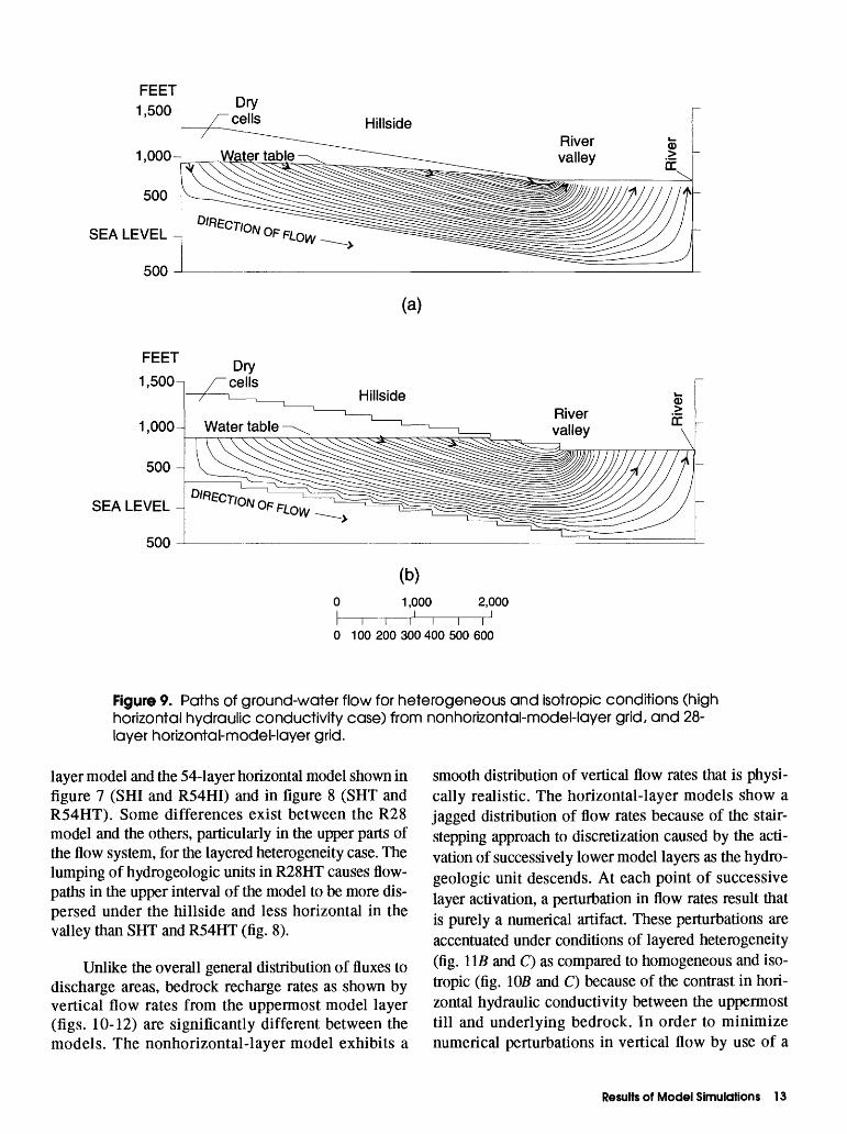
9. Heterogeneous and isotropic conditions (high horizontal hydraulic conductivity case) fromnonhorizontal-model-layer grid, and 28-layer horizontal-model-layer grid......................................... 13

10-12. Graphs showing distribution of vertical flow between bedrock and glacial drift for:10. Homogeneous and isotropic conditions from nonhorizontal-model-layer grid, 28-layer

horizontal-model-layer grid, and 54-layer horizontal-model-layer grid............................................... 1411. Heterogeneous and isotropic conditions from nonhorizontal-model-layer grid, 28-layer

horizontal-model-layer grid, and 54-layer horizontal-model-layer grid............................................... 1512. Heterogeneous and isotropic conditions (high horizontal hydraulic conductivity case) from

nonhorizontal-model-layer grid and 28-layer horizontal-model-layer grid.......................................... 1613-15. Graphs showing distribution of simulated head from lowest active model layer for:

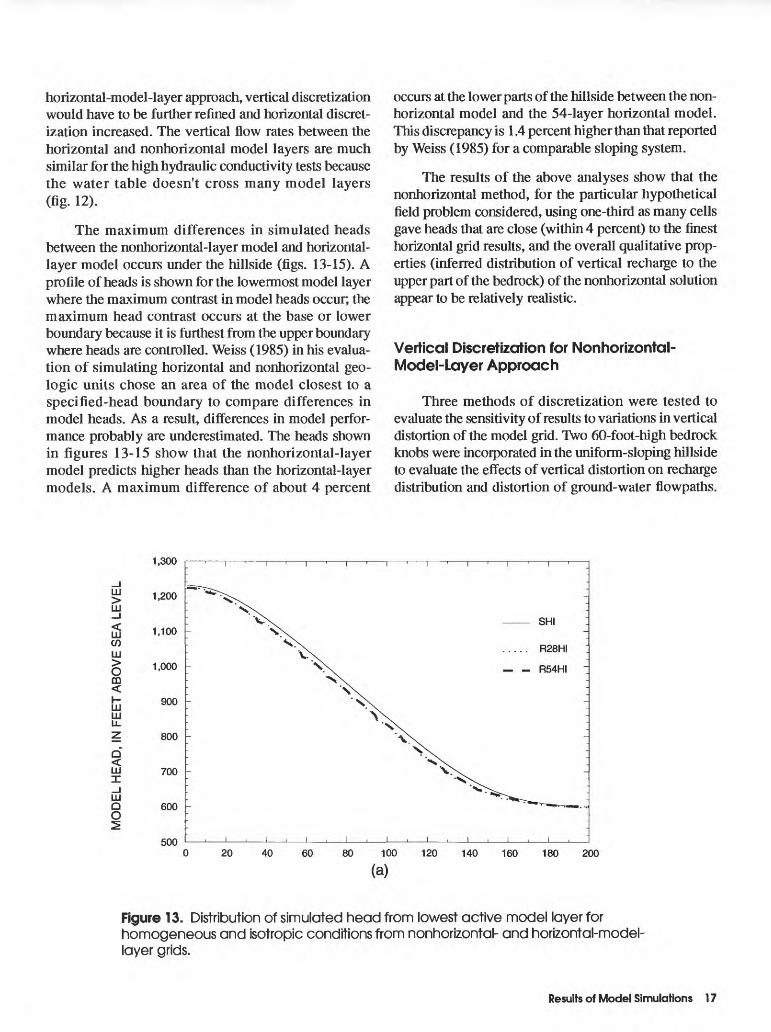
13. Homogeneous and isotropic conditions from nonhorizontal- and horizontal-model- layer grids.............................................................................................................................................. 17

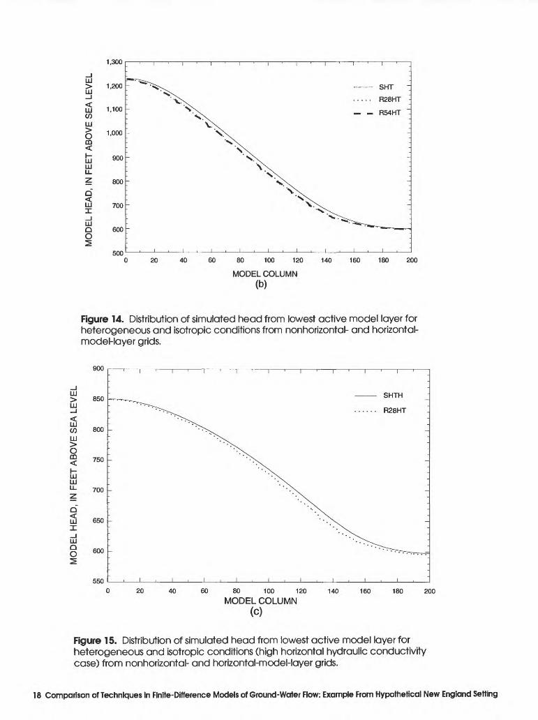
14. Heterogeneous and isotropic conditions from nonhorizontal- and horizontal-model- layer grids.............................................................................................................................................. 18

15. Heterogeneous and isotropic conditions (high horizontal hydraulic conductivity case)from nonhorizontal- and horizontal-model-layer grids......................................................................... 18

16-18. Vertical section showing model grid and paths of ground-water flow for simulated bedrock knobs with:

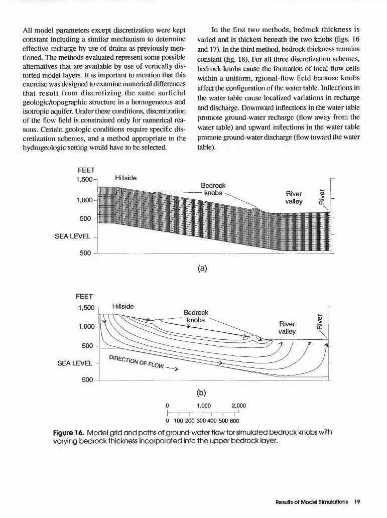
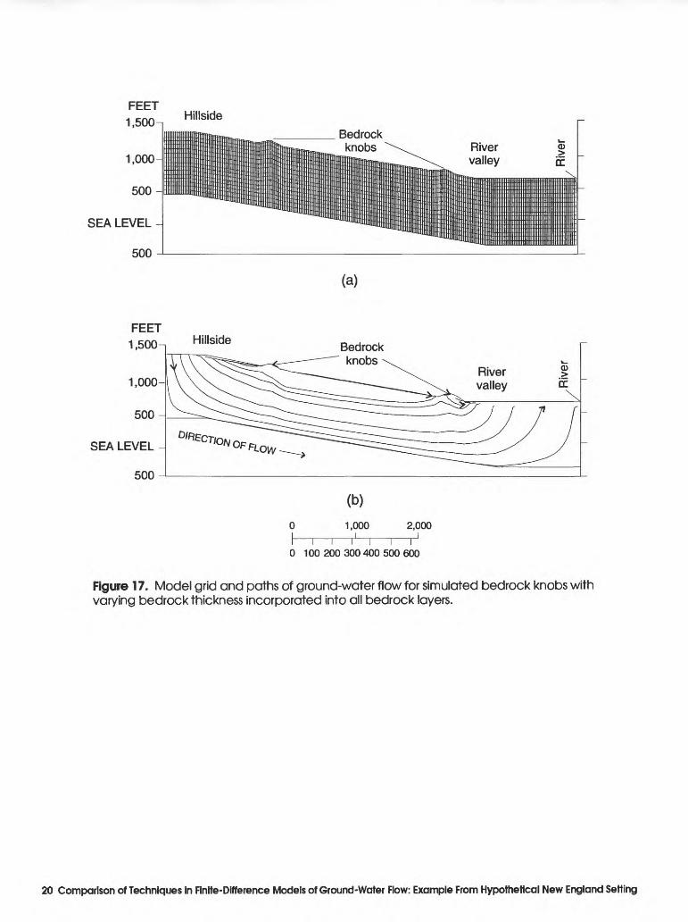
16. Varying bedrock thickness incorporated into the upper bedrock layer....................................................... 1917. Varying bedrock thickness incorporated into all bedrock layers................................................................ 2018. Constant bedrock thickness ........................................................................................................................ 21

19. Schematic diagrams showing a sloping hydrogeologic unit, a nonhorizontal-model-layer representation of the sloping unit, and a particle-tracking approach for a nonhorizontal- model-layer grid............................................................................................................................................. 22

20. Graph showing distribution of vertical flow between bedrock and glacial drift for simulatedbedrock knobs ................................................................................................................................................ 23

Contents Hi

TABLES

1. Distribution of major ground-water discharge patterns for vertical discretization tests on nonhorizontal- and horizontal-model-layer grids............................................................

2. Distribution of major ground-water discharge patterns for vertical discretization tests on bedrock knobs .................................................................................................................

10

22

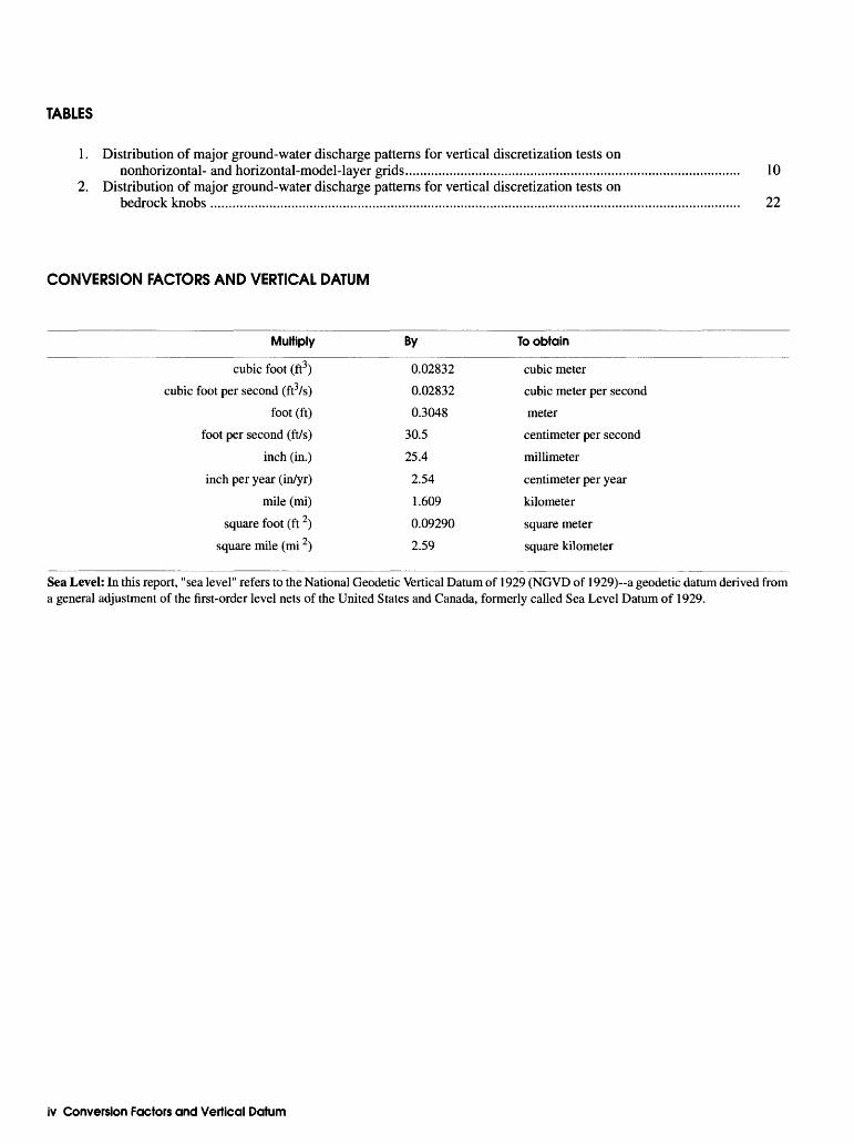
CONVERSION FACTORS AND VERTICAL DATUM

Multiply

cubic foot (ft3)

cubic foot per second (ft3/s)

foot (ft)

foot per second (ft/s)

inch (in.)

inch per year (in/yr)

mile (mi)

square foot (ft 2)

square mile (mi 2)

By

0.02832

0.02832

0.3048

30.5

25.4

2.54

1.609

0.09290

2.59

To obtain

cubic meter

cubic meter per second

meter

centimeter per second

millimeter

centimeter per year

kilometer

square meter

square kilometer

Sea Level: In this report, "sea level" refers to the National Geodetic Vertical Datum of 1929 (NGVD of 1929)~a geodetic datum derived from a general adjustment of the first-order level nets of the United States and Canada, formerly called Sea Level Datum of 1929.

iv Conversion Factors and Vertical Datum

Comparison of Vertical Discretization Techniques in Finite-Difference Models of Ground-Water Flow: Example From a Hypothetical New England Setting

By Philip T. Harte

Abstract

Proper discretization of a ground-water-flow field is necessary to provide adequate representation of a physical hydrogeologic system by numerical models. Some guidelines are available to ensure numerical sta bility, but current guidelines are flexible enough (par ticularly in vertical discretization) to allow for some ambiguity of simulation results. The finite-difference ground-water-flow equations used by many numerical models assume a horizontal-model-layer grid and rect angular cell faces. A horizontal-model-layer grid in the vertical section commonly leads to many model layers and cumbersome data input. To reduce data input, some finite-difference models allow for nonhorizontal- model layers and (or) vertical distortion of model cells to conform to hydrogeologic-unit slope and thickness but they may not incorporate the necessary mathemat ical terms to correct for the vertical misalignment of adjacent cells. These alternative discretization schemes, while introducing some numerical error, offer an improved physical representation of the system and minimize model-data input.

Several vertical-discretization tests on the same hypothetical representation of a hillside-valley terrain of New England revealed relatively small differences associated with horizontal-layer models and nonhorizontal-layer models in representing moderately sloping (0.17 foot per foot) hydrogeologic units. The numerical errors introduced by use of a nonhorizontal- model-layer grid because of the misalignment of model axes with the hydraulic conductivity tensor are small relative to advantages gained in improved representa tion of the flow system. The nonhorizontal grid results showed an inferred distribution of vertical recharge to the upper part of the bedrock that appears to be more

realistic than results from the horizontal grids tested. Further testing of discretization procedures by use of a nonhorizontal-layered model with vertical distortion of model cells showed that vertical distortion is a useful tool in approximating some geologic features.

INTRODUCTION

The ability of a numerical model to provide cor rect solutions to ground-water-flow problems is com monly evaluated by comparing results from the numerical model of interest with results from analytical models. However, because complex aquifer geometries and heterogeneities may not have analytical solutions, verification of numerical results by comparing against analytical solutions is not possible. Because numerical methods solve for head or stream function at a discrete point and do not provide a continuous solution like analytical methods do, proper discretization of the solution domain into a model grid is important to ensure accurate results. In the absence of verification options with analytical solutions, numerical model performance must be judged by testing various discretization schemes. Numerical results can then be evaluated by comparing consistency among various discretization schemes and adequacy of solution convergence for the various models. The characteris tics and rate of solution convergence (how well conver gence proceeds) is important in determining the acceptability of spatial and temporal discretization schemes (Trescott and others, 1976; Huyakorn and Finder, 1983).

Even within numerical stability guidelines, dis cretization practices are flexible enough to produce differences in model results. These diferences are

Introduction 1

commonly the result of variations in vertical discretization, variation in model-layer assignment of hydrogeologic units, and incorrect conceptual representation of the physical system.

The finite-difference method is computationally convenient if vertical discretization of the flow domain is in horizontal model layers and rectangular cells. As a result, most finite-difference numerical codes like MODFLOW (McDonald and Harbaugh, 1988) compute flow based on the assumption of horizontal model layers with cells of uniform rectangular shape. Because of the complex configuration of a three- dimensional distribution of hydrogeologic units, such as sloping or inclined units with nonuniform thickness, vertical discretization by use of horizontal model layers sometimes cannot create an accurate physical model of the stratigraphy without requiring an unreasonably fine grid.

Nonhorizontal model layers and (or) vertical dis tortion of model cells commonly are used in three- dimensional and cross-sectional models to compensate for the limitations of horizontal layer, rectangular dis cretization. Nonhorizontal model layers approximate a sloping hydrogeologic unit by means of a nonuniform vertical position of a model layer. Vertical distortion deforms a cell in the vertical direction to match thick nesses of hydrogeologic units (McDonald and Har baugh, 1988) and can lead to nonhorizontal layer cells. Each of these methods can be used to reduce the number of model cells and layers.

Although it has been acknowledged that with the nonhorizontal-layer approach some numerical accuracy is sacrificed to produce an improved conceptual repre sentation of the physical system (McDonald and Har baugh, 1988), little experimentation has been done to assess the ramifications of these discretization practices on error in model results. Weiss (1985) did a numerical study examining the differences of ground-water flow between horizontal stratigraphic units and synclinal stratigraphic units. In it he used variations in discretiza tion of the horizontal-model-layer approach to test the formulation of flow equations from a curvilinear grid system earlier described by Aziz and Settari (1979). However, he did not investigate the effect of discretiza tion refinements and the effects of model-layer assignment on model results.

This paper describes some numerical tests that were done to assess effects of nonhorizontal-layer- model grids and various vertical-distortion practices on results of simulations made using cross-sectional, finite- difference, steady-state models of a hypothetical hill side environment in New England. The U.S. Geological Survey finite-difference numerical model MODFLOW (McDonald and Harbaugh, 1988) was used because of its universal application to approximate various bound ary conditions and stresses and because of a post processing interface, MODPATH, that allows for particle tracking (Pollock, 1989). MODPATH is a semi- analytical particle-tracking scheme that uses heads computed by MODFLOW, assigned hydraulic conduc tivities, and a linear-tracking algorithm to move parti cles. MODPATH can accommodate various vertical- discretization approaches. A technique of vertically routing or tracking particles through inclined model layers is discussed by Pollock (1989).

Numerical test results in this paper include a com parison of model output (head distributions, ground- water flow, and ground-water budgets) from a horizontal-layer model with an inclined or sloping, nonhorizontal-layer model. Some additional numerical tests also are included to assess vertical-distortion practices by use of a nonhorizontal-layer model. These tests involve variations in vertical-distortion practices associated with representing a particular geologic feature.

CONSIDERATIONS IN VERTICAL DISCRETIZATION OF FINITE- DIFFERENCE MODELS

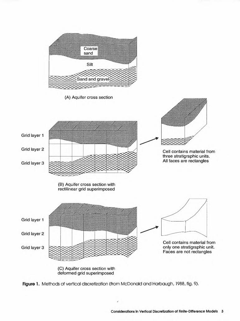
Two contrasting vertical-discretization schemes are permissible in MODFLOW corresponding to the horizontal- and nonhorizontal-model-layer approach (fig. 1). The horizontal approach involves dividing the flow system into horizontal segments along the vertical (fig. \B). The nonhorizontal approach attempts to con form individual stratigraphic or hydrogeologic units into discrete model layers (fig. 1C).

According to McDonald and Harbaugh (1988, p. 2-31):

Each of these methods of viewing the vertical-discretization process has advantages, and each presents difficulties. The model

2 Comparison of Techniques in Finite-Difference Models of Ground-Water Flow: Example From Hypothetical New England Setting

Grid layer 1

Grid layer 2

Grid layer 3

Grid layer 1

Grid layer 2

Grid layer 3

(A) Aquifer cross section

(B) Aquifer cross section with rectilinear grid superimposed

Cell contains material from three stratigraphic units. All faces are rectangles

Cell contains material from only one stratigraphic unit. Faces are not rectangles

(C) Aquifer cross section with deformed grid superimposed

Figure 1. Methods of vertical discretization (from McDonald and Harbaugh, 1988, fig. 9).

Considerations In Vertical Discretization of Finite-Difference Models 3

equations are based on the assumption that hydraulic properties are uniform within individ ual cells, or at least that meaningful average or integrated parameters can be specified for each cell; these conditions are more likely to be met when model layers conform to geohydrologic units (fig. 1C). Moreover, greater accuracy can be expected if model layers correspond to inter vals within which vertical head loss is negligible (fig. 1C). On the other hand, the deformed grid fails to conform to many of the assumptions upon which the model equations are based; for example, individual cells may no longer have rectangular faces, and the major axes of hydrau lic conductivity may not be aligned with the model axis. Some error is always introduced by these departures from assumed conditions.

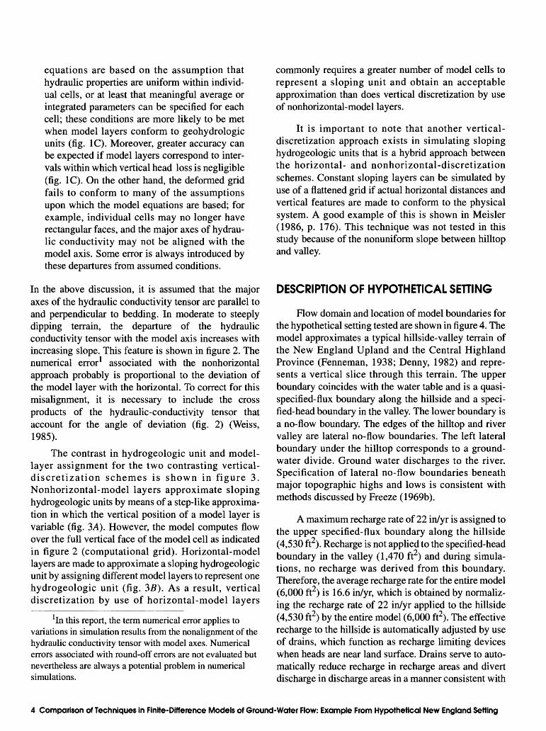
In the above discussion, it is assumed that the major axes of the hydraulic conductivity tensor are parallel to and perpendicular to bedding. In moderate to steeply dipping terrain, the departure of the hydraulic conductivity tensor with the model axis increases with increasing slope. This feature is shown in figure 2. The numerical error 1 associated with the nonhorizontal approach probably is proportional to the deviation of the model layer with the horizontal. To correct for this misalignment, it is necessary to include the cross products of the hydraulic-conductivity tensor that account for the angle of deviation (fig. 2) (Weiss, 1985).

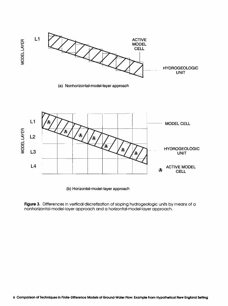
The contrast in hydrogeologic unit and model- layer assignment for the two contrasting vertical- discretization schemes is shown in figure 3. Nonhorizontal-model layers approximate sloping hydrogeologic units by means of a step-like approxima tion in which the vertical position of a model layer is variable (fig. 3A). However, the model computes flow over the full vertical face of the model cell as indicated in figure 2 (computational grid). Horizontal-model layers are made to approximate a sloping hydrogeologic unit by assigning different model layers to represent one hydrogeologic unit (fig. 3B). As a result, vertical discretization by use of horizontal-model layers

In this report, the term numerical error applies to variations in simulation results from the nonalignment of the hydraulic conductivity tensor with model axes. Numerical errors associated with round-off errors are not evaluated but nevertheless are always a potential problem in numerical simulations.

commonly requires a greater number of model cells to represent a sloping unit and obtain an acceptable approximation than does vertical discretization by use of nonhorizontal-model layers.

It is important to note that another vertical- discretization approach exists in simulating sloping hydrogeologic units that is a hybrid approach between the horizontal- and nonhorizontal-discretization schemes. Constant sloping layers can be simulated by use of a flattened grid if actual horizontal distances and vertical features are made to conform to the physical system. A good example of this is shown in Meisler (1986, p. 176). This technique was not tested in this study because of the nonuniform slope between hilltop and valley.

DESCRIPTION OF HYPOTHETICAL SETTING

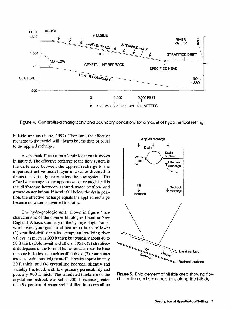
Flow domain and location of model boundaries for the hypothetical setting tested are shown in figure 4. The model approximates a typical hillside-valley terrain of the New England Upland and the Central Highland Province (Fenneman, 1938; Denny, 1982) and repre sents a vertical slice through this terrain. The upper boundary coincides with the water table and is a quasi- specified-flux boundary along the hillside and a specified-head boundary in the valley. The lower boundary is a no-flow boundary. The edges of the hilltop and river valley are lateral no-flow boundaries. The left lateral boundary under the hilltop corresponds to a ground- water divide. Ground water discharges to the river. Specification of lateral no-flow boundaries beneath major topographic highs and lows is consistent with methods discussed by Freeze (1969b).

A maximum recharge rate of 22 in/yr is assigned to the upper specified-flux boundary along the hillside (4,530 ft ). Recharge is not applied to the specified-head boundary in the valley (1,470 ft ) and during simula tions, no recharge was derived from this boundary. Therefore, the average recharge rate for the entire model (6,000 ft ) is 16.6 in/yr, which is obtained by normaliz ing the recharge rate of 22 in/yr applied to the hillside (4,530 ft2) by the entire model (6,000 ft2). The effective recharge to the hillside is automatically adjusted by use of drains, which function as recharge limiting devices when heads are near land surface. Drains serve to auto matically reduce recharge in recharge areas and divert discharge in discharge areas in a manner consistent with


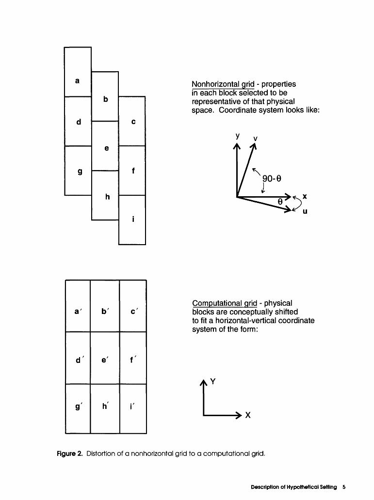
Nonhorizontal grid - properties in each block selected to be representative of that physical space. Coordinate system looks like:

Computational grid - physical blocks are conceptually shifted to fit a horizontal-vertical coordinate system of the form:

Figure 2. Distortion of a nonhorizontal grid to a computational grid.

Description of Hypothetical Setting 5

ccLU

LU O O

L1 ACTIVEMODELCELL

HYDROGEOLOGIC UNIT

(a) Nonhorizontal-model-layer approach

ccLU

Q O

L1

L2

L3

L4

MODEL CELL

HYDROGEOLOGIC UNIT

ACTIVE MODEL CELL

(b) Horizontal-model-layer approach

Figure 3. Differences in vertical discretization of sloping hydrogeologic units by means of a nonhorizontal-model-layer approach and a horizontal-model-layer approach.


FEET HILLTOP

1,500-| HILLSIDE

i 7*70*1*L i i

RIVER £ VALLEY |

STRATIFIED DRIFT

SEA LEVEL

500

CRYSTALLINE BEDROCK

1,000 2,000 FEET

IIr i r ir^0 100 200 300 400 500 600 METERS

Figure 4. Generalized stratigraphy and boundary conditions for a model of hypothetical setting.

hillside streams (Harte, 1992). Therefore, the effective recharge to the model will always be less than or equal to the applied recharge.

A schematic illustration of drain locations is shown in figure 5. The effective recharge to the flow system is the difference between the applied recharge to the uppermost active model layer and water diverted to drains that virtually never enters the flow system. The effective recharge to any uppermost active model cell is the difference between ground-water outflow and ground-water inflow. If heads fall below the drain posi tion, the effective recharge equals the applied recharge because no water is diverted to drains.

The hydrogeologic units shown in figure 4 are characteristic of the diverse lithologies found in New England. A basic summary of the hydrogeologic frame work from youngest to oldest units is as follows: (1) stratified-drift deposits occupying low lying river valleys, as much as 200 ft thick but typically about 40 to 50 ft thick (Goldthwait and others, 1951), (2) stratified- drift deposits in the form of kame terraces near the base of some hillsides, as much as 40 ft thick, (3) continuous and discontinuous lodgment-till deposits approximately 20 ft thick, and (4) crystalline bedrock, slightly and variably fractured, with low primary permeability and porosity, 900 ft thick. The simulated thickness of the crystalline bedrock was set at 900 ft because greater than 99 percent of water wells drilled into crystalline

Applied recharge

4r . . 4r

Water Jtable X V x

Till *

Bedrock

> Drain outflow

Effective recharge^^->

BedrockV recharge

Land surface

Bedrock surface

Figure 5. Enlargement of hillside area showing flow distribution and drain locations along the hillside.

Description of Hypothetical Setting 7

rock are drilled to depths less than 900 ft (Chorman, 1990). A detailed discussion of physical setting and conceptual flow system is given in Harte (1992).

NUMERICAL MODELS OF HYPOTHETICAL SETTING

Numerical simulations of the hypothetical setting were solved by use of iterative matrix solvers: either the preconditioned-conjugate-gradient solver (Hill, 1990) or the slice-successive-overrelaxation technique (McDonald and Harbaugh, 1988). A convergence criterion of 0.01 ft is used between successive iterations.

All model cells, except constant-head cells in the river valley along the upper model boundary, are simu lated as variable-head cells. In MODFLOW, flow in cells from the upper model layers are solved by use of an unconfined finite-difference flow equation to account for partially wet cells. Flow in cells from the remaining layers is solved by use of a confined finite-difference flow equation unless heads decline below the base of the upper layers. If heads decline below the altitude of the top face of a cell, flow is converted from confined to unconfined. An updated version of MODFLOW was used to allow for resaturation of cells during iterative solution for when numerical oscillation cause prema ture desaturation (McDonald and others, 1991). Numer ical oscillation can cause computed heads for some solution iterations to decline below the base of the cell even though some of the computed heads for the final iteration of that same simulation period or step may be above the top of the cell.

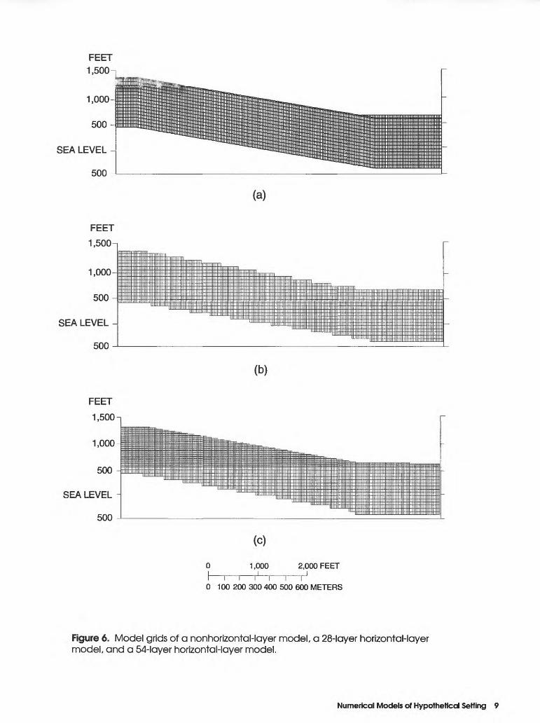
Three finite-difference models were constructed of the hypothetical New England setting to test the effects of vertical-discretization schemes on simulated flow (fig. 6). The three models include a nonhorizontal- model-layer grid (abbreviated S, fig. 6A) and two horizontal-model-layer grids, a 28-layer grid (abbrevi ated R28, fig. 6B) and a 54-layer grid (abbreviated R54, fig. 6Q. Horizontal model dimensions and grid spacing are identical for all three grids. Vertical discretization and model-layer assignment are different. The model- input requirements increase in complexity from the nonhorizontal-model-layer grid to the 54-layer horizontal grid.

The nonhorizontal-model-layer grid is vertically discretized into 17 model layers; the upper two layers are 50 and 20 ft thick, respectively; the lower 15 layers are each 60 ft thick. Multiple bedrock model layers are used to ensure numerical accuracy and provide high vertical resolution of flow. The hydrogeologic units are discretized as follows: (1) layer 1 is present only in the valley, and it simulates a 5 0-foot-thick stratified drift, (2) layer 2 is continuous, and it simulates a 20-foot- thick lodgment till, and (3) layers 3 through 17 simulate the bedrock, which has a total modeled thickness of 900 ft.

The horizontal-model-layer grids have different model layer assignments of hydrogeologic units. The 28-layer model is vertically discretized into 60-foot- thick layers and contains approximately the same number of active cells as the nonhorizontal-layer model. Because the number of cells and model layers were kept the same as the nonhorizontal-model-layer grid, the stratified drift and till could not be assigned to discrete layers and had to be incorporated with the bedrock into the upper 13, uniformly discretized 60-foot-thick layers. This deficiency requires the hydraulic parame ters from multiple hydrogeologic units to be lumped into a single model layer. The 54-layer model is verti cally discretized into thirty-seven 20-foot-thick layers in the upper part of the model so that the till could be assigned to discrete model layers; the lower 17 model layers are 60 ft thick and represent the bedrock. There fore, the effects of lumping of hydraulic parameters can be evaluated by comparing results of these two models.

For the 28-layer horizontal-layer model, the hori zontal hydraulic conductivity of the till and bedrock were incorporated into the uppermost active layer, from layers 1-12, to simulate the sloping hydrogeologic units along the hillside. Lumped horizontal hydraulic con ductivities of till and bedrock were calculated by use of a weighted average of the till and bedrock thickness within each model layer. The horizontal hydraulic con ductivities of the stratified drift and till in the valley were incorporated in layer 13 in the valley by similar procedures.

Use of the weighted-average technique causes a less precise physical representation of the system and therefore, is a deficiency of the 28-layer-model grid. Horizontal hydraulic conductivity is computed by assuming that flow within a model layer is parallel to the slope of the hydrogeologic unit. If difference in


FEET

1,500 n

1,000

500-

SEA LEVEL -

500

(a)

(b)

(c)

1,000 2,000 FEET

i i i i i i r0 100 200 300 400 500 600 METERS

Figure 6. Model grids of a nonhorizontal-layer model, a 28-layer horizontal-layer model, and a 54-layer horizontal-layer model.

Numerical Models of Hypothetical Setting 9

permeabilities between two dissimilar units, such as between stratified drift and till are significant, the phys ical representation of these units will be less precise than if units were assigned to discrete model layers. The lack of precision causes a problem in distribution of flow and precludes determination of the amount of recharge to a specific unit. Vertical hydraulic conductiv ity of the vertical hydrogeologic sequence of lumped units is governed by the least permeable unit of the sequence.

RESULTS OF MODEL SIMULATIONS

Model results were compared by examining the distribution of (1) ground-water flowpaths generated from particle tracking to track regional flow, (2) outflow to hillside streams and the river valley, (3) bedrock recharge, and (4) heads. Paths of ground-water flow were generated by moving particles in a frontward- tracking scheme, from recharge to discharge areas, or a backward-tracking scheme, from discharge to recharge areas. Bedrock recharge equals the applied recharge minus water diverted to drains (hillside streams) and lateral flow in the till.

Comparison of Horizontal-Model-Layer and Nonhorizontal-Model-Layer Approach

The model runs tested to compare vertical- discretization schemes are divided into homogeneous and isotropic (abbreviated HI) and layered heteroge neous and isotropic (abbreviated HT). Each group contains three different discretized models the nonhorizontal-layered model (abbreviated S), and two horizontal-layer models (abbreviated R28 for the 28-layered model and R54 for the 54-layer model). The significant difference in the R28 and R54 layered model is that the till unit, which is 20 ft thick, can be discretely represented in the 54-layer model instead of lumped together with the bedrock as in the 28-layer model. This problem is avoided in the nonhorizontal-layer model because each model layer conforms to the hydogeologic unit position.

The homogeneous and isotropic runs have a uni form hydraulic conductivity of 0.16x10 ft/s. These runs should eliminate the effect of lumping of multiple hydrogeologic units into one model layer, which happens in R28. The layered heterogeneous runs

contain the permeability distribution associated with the stratified drift (0.4xl(T4 ft/s), till (0.13xl(T5 ft/s), and bedrock (0.16xlO'6 ft/s).

The differences in major discharge patterns are small (table 1) and show no significant variation between model runs. Refinement of the horizontal lay ered model from 28 to 54 model layers makes little dif ference. For all models, layered heterogeneity increases flow to the river valley because of the presence of the permeable stratified-drift deposits.

Additional analyses were performed on the effects of layered heterogeneity by increasing the horizontal hydraulic conductivity of the bedrock (0.328xlO~5 ft/s) by using the nonhorizontal-layer model and the 28-layer horizontal model. This results in a much lower ratio of hillside to valley discharge and a greater dissimilarity between the two cases than that shown in table 1. The ratio of discharge is much less for model R28HT (0.1) than SHI (0.6). Under these conditions because the hydraulic-head gradient is shallow and is only close to land surface for a small part of the lower hillside, the differences in discretization technique is important.

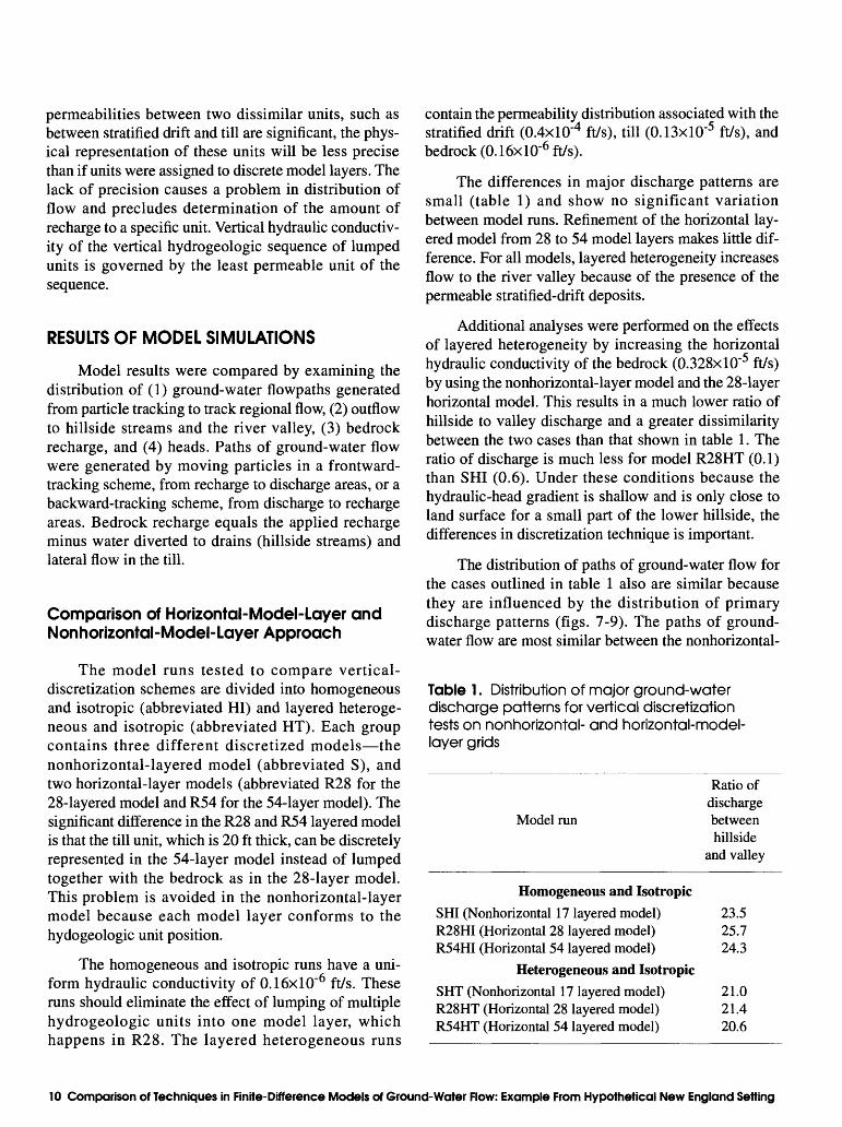
The distribution of paths of ground-water flow for the cases outlined in table 1 also are similar because they are influenced by the distribution of primary discharge patterns (figs. 7-9). The paths of ground- water flow are most similar between the nonhorizontal-

Table 1 . Distribution of major ground-water discharge patterns for vertical discretization tests on nonhorizontal- and horizontal-model- layer grids

Model run

Ratio ofdischargebetweenhillside

and valley

Homogeneous and IsotropicSHI (Nonhorizontal 17 layered model) 23.5R28HI (Horizontal 28 layered model) 25.7R54HI (Horizontal 54 layered model) 24.3

Heterogeneous and IsotropicSHT (Nonhorizontal 17 layered model) 21.0R28HT (Horizontal 28 layered model) 21.4R54HT (Horizontal 54 layered model) 20.6


(a)

(b)

(c)

1,000 2,000 FEET

0 100 200 300 400 500 600 METERS

Figure 7. Paths of ground-water flow for homogeneous and isotropic conditions from nonhorizontal-model-layer grid, 28-layer horizontal-model-layer grid, and 54-layer horizontal-model-layer grid.

Results of Model Simulations 11

(a)

(b)

(c)1,000 2,000 FEET

I I I I I I 0 100 200 300 400 500 600 METERS

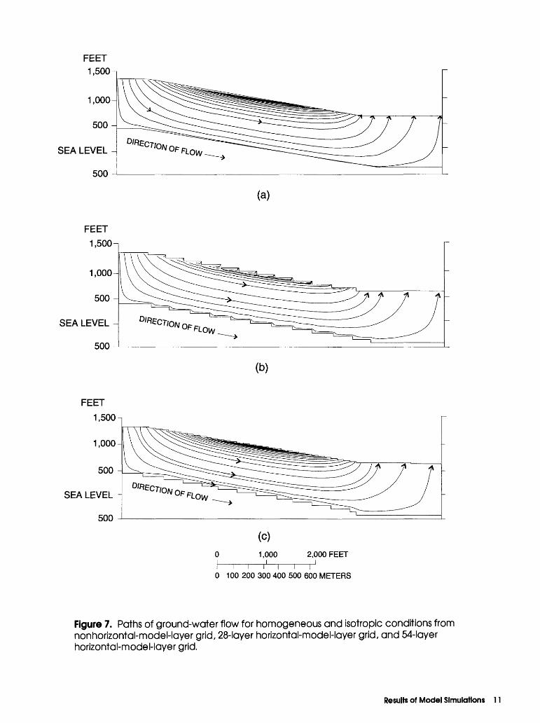
Figure 8. Paths of ground-water flow for heterogeneous and isotropic conditions from nonhorizontal-model-layer grid, 28-layer horizontal-model-layer grid, and 54-layer horizontal-model-layer grid.


(a)

500

(b)1,000 2,000

IIII I \ \^ 0 100200300400500600

Figure 9. Paths of ground-water flow for heterogeneous and isotropic conditions (high horizontal hydraulic conductivity case) from nonhorizontal-model-layer grid, and 28- layer horizontal-model-layer grid.

layer model and the 54-layer horizontal model shown in figure 7 (SHI and R54HI) and in figure 8 (SHT and R54HT). Some differences exist between the R28 model and the others, particularly in the upper parts of the flow system, for the layered heterogeneity case. The lumping of hydrogeologic units in R28HT causes flowpaths in the upper interval of the model to be more dis persed under the hillside and less horizontal in the valley than SHT and R54HT (fig. 8).

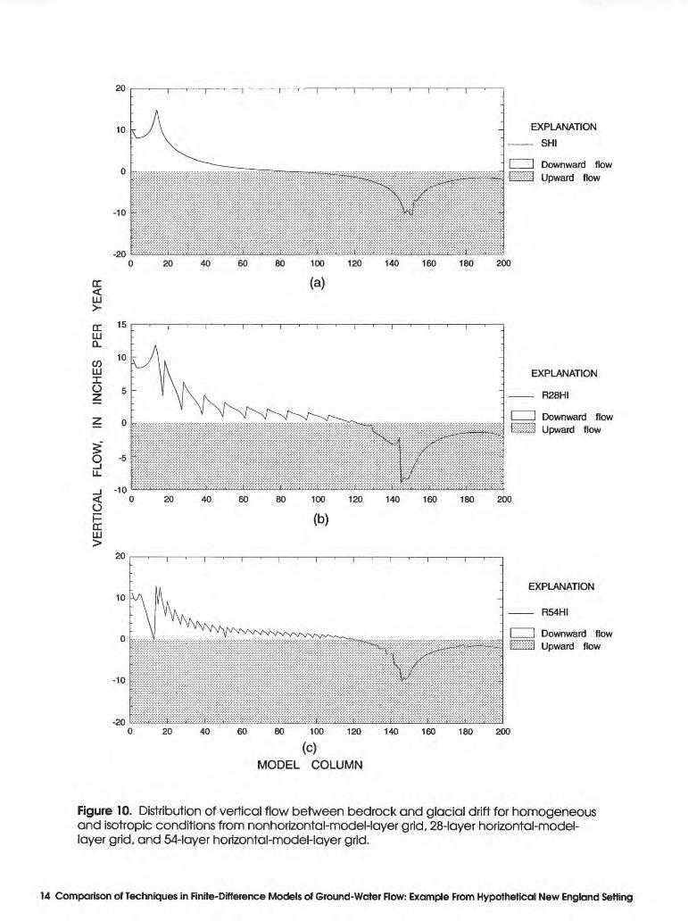
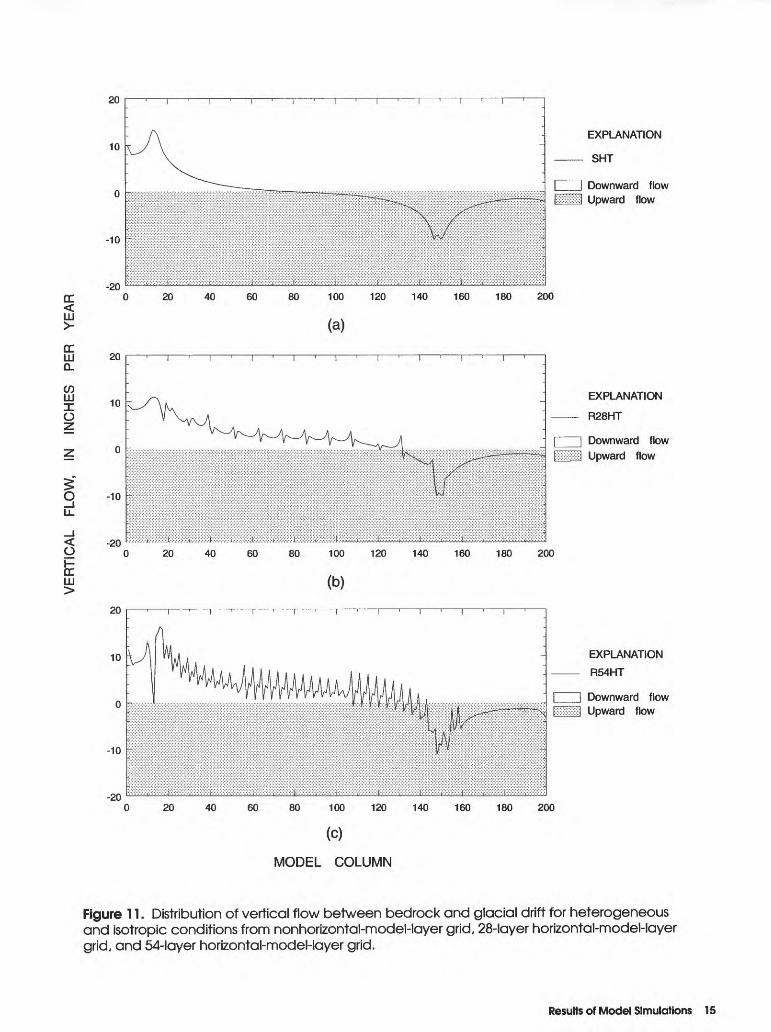
Unlike the overall general distribution of fluxes to discharge areas, bedrock recharge rates as shown by vertical flow rates from the uppermost model layer (figs. 10-12) are significantly different between the models. The nonhorizontal-layer model exhibits a

smooth distribution of vertical flow rates that is physi cally realistic. The horizontal-layer models show a jagged distribution of flow rates because of the stair stepping approach to discretization caused by the acti vation of successively lower model layers as the hydrogeologic unit descends. At each point of successive layer activation, a perturbation in flow rates result that is purely a numerical artifact. These perturbations are accentuated under conditions of layered heterogeneity (fig. IIB and C) as compared to homogeneous and iso tropic (fig. WB and C) because of the contrast in hori zontal hydraulic conductivity between the uppermost till and underlying bedrock. In order to minimize numerical perturbations in vertical flow by use of a


20

10

-10

-20

CC < 111

o: 15LLJCL

20 40 60 80 100 120 140

(a)160 180 200

co111X

10

O -5

-10

O

CC LLJ

(b)

-20 ! f !

0 20 40 60 80 100 120 140

(c)

MODEL COLUMN

20 40 60 80 100 120 140 160 180 200

EXPLANATION

SHI

I Downward flow:l Upward flow

EXPLANATION

- R28HI

Downward flow fcffff&l Upward flow

EXPLANATION

R54HI

Downward flow Wm\ Upward flow

160 180 200

Figure 10. Distribution of vertical flow between bedrock and glacial drift for homogeneous and isotropic conditions from nonhorizontal-model-layer grid, 28-layer horizontal-model- layer grid, and 54-layer horizontal-model-layer grid.


cc <LLJ

o:LJJ Q.

(f)LJJI Oz

o

< o

LJJ >

20

10

-10

-20 ""

20

10

-10

-20

80 100 120 140 160 180 200

(a)

0 20 40 60 80 100

(b)

n ' r i i

120 140 160 180 200

20 40 60 80 100 120 140 160 180

(C)

MODEL COLUMN

200

EXPLANATION

SHT

Downward flow Upward flow

EXPLANATION

R28HT


EXPLANATION

R54HT


Figure 11 . Distribution of vertical flow between bedrock and glacial drift for heterogeneous and isotropic conditions from nonhorizontal-model-layer grid, 28-layer horizontal-model-layer grid, and 54-layer horizontal-model-layer grid.


w20

0

-20

-40

-60

LL

LLI>- -100

OCLLI -120 QL

C/D -140 LLI

0 -160

:= (

^

O1 1 -inn

ERTICAL F

g i

^

0

-50

-100

-150

£.\J\J

| , | , | , | , | i , , |

\^^^^^^^^^

^^K^mii^^^^^^^^^^M^^^^m.

j* - - - - "^X;X;X ;!;!;! ;!;!;!;!;X;X;!;!;!;!;!;!;X;!;X^ [

*r XvX'XvXvXvXvXvX'X'X'X-XvX-XvXvXvXvX i

' ' ' ' ' ' ' ' ' ' ' ' ' ' ':;:;:;;;:;:;:;:;:;:;:;:;:;:;:;:;:;:;:;:;:;

I*

) 20 40 60 80 100 120 140

(a)

I I I . I I I < I I I I

? ^^mt^MZXMi^* ': :::::::::: :: :: :: :: : : :: i: : :: : :: :: :: :: :: :: :: :: :: :: :: :: :::: :: :: :: :: :: :: :::: :: :: :: :: :: :: :: :: :: :: :: :: :: :: :^^^^^^^

- J f

3 20 40 60 80 100 120 140

i , i i

^^f^mm^m^m^m

^k f- f;

S I / 1

;.-

J :

.. / \

:

V T 1 , 1160 180 2(

I '

mmmmmmmmm

rff ^

/ 1

$ ii !

160 180 2

EXPLANATION

SHTH

I I Downward flow fc£x£:l Upward flow

)0

EXPLANATION

DOQLJTLJ

I I Downward flow I££S£;I Upward flow

30

(b)

MODEL COLUMN

Figure 12. Distribution of vertical flow between bedrock and glacial drift for heterogeneous and isotropic conditions (high horizontal hydraulic conductivity case) from nonhorizontal-model-layer grid and 28-layer horizontal-model-layer grid.


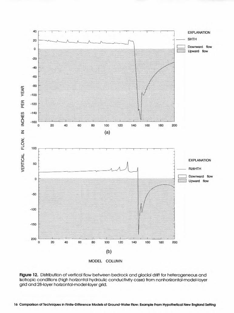
horizontal-model-layer approach, vertical discretization would have to be further refined and horizontal discret ization increased. The vertical flow rates between the horizontal and nonhorizontal model layers are much similar for the high hydraulic conductivity tests because the water table doesn't cross many model layers (fig. 12).

The maximum differences in simulated heads between the nonhorizontal-layer model and horizontal- layer model occurs under the hillside (figs. 13-15). A profile of heads is shown for the lowermost model layer where the maximum contrast in model heads occur; the maximum head contrast occurs at the base or lower boundary because it is furthest from the upper boundary where heads are controlled. Weiss (1985) in his evalua tion of simulating horizontal and nonhorizontal geo logic units chose an area of the model closest to a specified-head boundary to compare differences in model heads. As a result, differences in model perfor mance probably are underestimated. The heads shown in figures 13-15 show that the nonhorizontal-layer model predicts higher heads than the horizontal-layer models. A maximum difference of about 4 percent

occurs at the lower parts of the hillside between the nonhorizontal model and the 54-layer horizontal model. This discrepancy is 1.4 percent higher than that reported by Weiss (1985) for a comparable sloping system.

The results of the above analyses show that the nonhorizontal method, for the particular hypothetical field problem considered, using one-third as many cells gave heads that are close (within 4 percent) to the finest horizontal grid results, and the overall qualitative prop erties (inferred distribution of vertical recharge to the upper part of the bedrock) of the nonhorizontal solution appear to be relatively realistic.

Vertical Discretization for Nonhorizontal- Model-Layer Approach

Three methods of discretization were tested to evaluate the sensitivity of results to variations in vertical distortion of the model grid. Two 60-foot-high bedrock knobs were incorporated in the uniform-sloping hillside to evaluate the effects of vertical distortion on recharge distribution and distortion of ground-water flowpaths.

LU

HI

LU<n LU§CO<tuLU

LUI _l LU O O

1,300

1,200

1,100

1,000

900

800

700

600

500

SHI

..... R28HI

- R54HI

20 40 60 80 100 120 140 160 180 200

(a)

Figure 13. Distribution of simulated head from lowest active model layer for homogeneous and isotropic conditions from nonhorizontal- and horizontal-model- layer grids.


1,300

HI> 1,200HI

HJ 1,100C/DHI

1,000oCO

HI

HII _J HI Q O

900

800

700

600

500

______ OUTon i

..... R28HT

R54HT

20 40 60 80 100 120

MODEL COLUMN

140 160 180 200

(b)

Figure 14. Distribution of simulated head from lowest active model layer for heterogeneous and isotropic conditions from nonhorizontal- and horizontal- model-layer grids.

HI >HI

900

850

HICfl 800

HI

OCO

HI

750

700

UJ 650I

HI Q O

600

550

20 40 60 80 100 120

MODEL COLUMN (C)

140

SHTH

R28HT

160 180 200

Figure 15. Distribution of simulated head from lowest active model layer for heterogeneous and isotropic conditions (high horizontal hydraulic conductivity case) from nonhorizontal- and horizontal-model-layer grids.

18 Comparison of Techniques In Finite-Difference Models of Ground-Water Flow: Example From Hypothetical New England Setting

All model parameters except discretization were kept constant including a similar mechanism to determine effective recharge by use of drains as previously men tioned. The methods evaluated represent some possible alternatives that are available by use of vertically dis torted model layers. It is important to mention that this exercise was designed to examine numerical differences that result from discretizing the same surficial geologic/topographic structure in a homogeneous and isotropic aquifer. Under these conditions, discretization of the flow field is constrained only for numerical rea sons. Certain geologic conditions require specific dis cretization schemes, and a method appropriate to the hydrogeologic setting would have to be selected.

In the first two methods, bedrock thickness is varied and is thickest beneath the two knobs (figs. 16 and 17). In the third method, bedrock thickness remains constant (fig. 18). For all three discretization schemes, bedrock knobs cause the formation of local-flow cells within a uniform, rgional-flow field because knobs affect the configuration of the water table. Inflections in the water table cause localized variations in recharge and discharge. Downward inflections in the water table promote ground-water recharge (flow away from the water table) and upward inflections in the water table promote ground-water discharge (flow toward the water table).

(a)

FEET

1,500-i Hillside . r

(b)1,000 2,000

I I I I I I I 0 100 200 300 400 500 600

Figure 16. Model grid and paths of ground-water flow for simulated bedrock knobs with varying bedrock thickness incorporated into the upper bedrock layer.


FEETHillside

(a)

(b)

1,000 2,000

I I 0 100 200 300 400 500 600

Figure 17. Model grid and paths of ground-water flow for simulated bedrock knobs with varying bedrock thickness incorporated into all bedrock layers.


FEET

1,500-i

1,000-

500-

SEA LEVEL -

500

HillsideBedrock knobs River

valley

(a)

FEET1,500-i Hillside

(b)

1,000 2,000

I I I I I I F 0 100 200 300 400 500 600

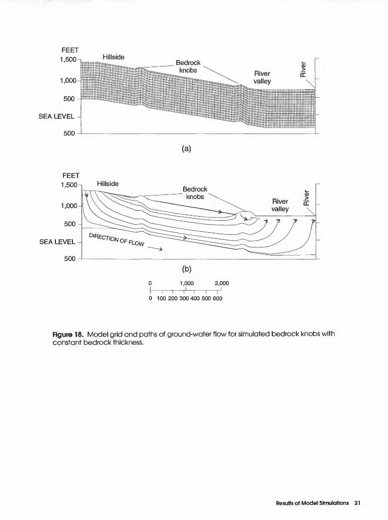
Figure 18. Model grid and paths of ground-water flow for simulated bedrock knobs with constant bedrock thickness.


In the first method, changes to the bedrock surface and the thickness of the flow field were restricted to the near surface by adjusting the thickness of the uppermost bedrock layer while maintaining the original thick nesses of the lower layers (fig. 16). Ground-water flowpaths are affected within the local-flow cell produced by the inflections of the water-table profile at bedrock knobs. Ground-water flowpaths within the regional- flow system also are affected below the local-flow cell to a depth of 200 ft. This effect is visible as a slight upward inflection or ripple in flowpaths under the local- discharge zone, on the upslope side of the bedrock knob. Ground-water flowpaths are unaffected in the remaining 700 ft. This method causes the least disturbance of flowpaths.

In the second method, changes to the bedrock sur face and the thickness of the flow field were incorpo rated into the entire flow field by adjusting the thickness of all modeled bedrock layers (fig. 17). Paths of ground- water flow within the regional-flow field are affected under the local-discharge zones at the upslope and downslope sides of knobs at greater depths than used in the first method. The second method causes a ripple effect in flowpaths within the regional-flow field, below the local-flow cell, to a depth of 700 ft below bedrock surface. This method causes an intermediate amount of disturbance of flowpaths.

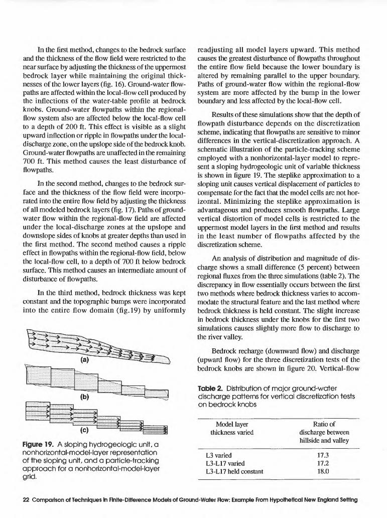
In the third method, bedrock thickness was kept constant and the topographic bumps were incorporated into the entire flow domain (fig. 19) by uniformly

(c)

Figure 19. A sloping hydrogeologic unit, a nonhorizontal-model-layer representation of the sloping unit, and a particle-tracking approach for a nonhorizontal-model-layer grid.

readjusting all model layers upward. This method causes the greatest disturbance of flowpaths throughout the entire flow field because the lower boundary is altered by remaining parallel to the upper boundary. Paths of ground-water flow within the regional-flow system are more affected by the bump in the lower boundary and less affected by the local-flow cell.

Results of these simulations show that the depth of flowpath disturbance depends on the discretization scheme, indicating that flowpaths are sensitive to minor differences in the vertical-discretization approach. A schematic illustration of the particle-tracking scheme employed with a nonhorizontal-layer model to repre sent a sloping hydrogeologic unit of variable thickness is shown in figure 19. The steplike approximation to a sloping unit causes vertical displacement of particles to compensate for the fact that the model cells are not hor izontal. Minimizing the steplike approximation is advantageous and produces smooth flowpaths. Large vertical distortion of model cells is restricted to the uppermost model layers in the first method and results in the least number of flowpaths affected by the discretization scheme.

An analysis of distribution and magnitude of dis charge shows a small difference (5 percent) between regional fluxes from the three simulations (table 2). The discrepancy in flow essentially occurs between the first two methods where bedrock thickness varies to accom modate the structural feature and the last method where bedrock thickness is held constant. The slight increase in bedrock thickness under the knobs for the first two simulations causes slightly more flow to discharge to the river valley.

Bedrock recharge (downward flow) and discharge (upward flow) for the three discretization tests of the bedrock knobs are shown in figure 20. Vertical-flow

Table 2. Distribution of major ground-water discharge patterns for vertical discretization tests on bedrock knobs

Model layer thickness varied

Ratio ofdischarge between hillside and valley

L3 varied L3-L17 varied L3-L17 held constant

17.317.218.0


20

10

-10

-20

-30

CC < LU

20 40 60 80 100 120 140 160 180 200

(a)

EXPLANATION

Knobs 13var

No knobs


CC LU CL

03 LUIo

o

5LJJ

20

10

-10

-20

20

10

EXPLANATION

___ Knobs13-117 var

No knobs


20 40 60 80 100 120 140 160 180 200

(b)

-10

-20

EXPLANATION

Knobs 13-117 const

No knobs

I I Downward flowf::S:&sl Upward flow

20 40 60 80 100 120 140 160 180 200

(c) MODEL COLUMN

Figure 20. Distribution of vertical flow between bedrock and glacial drift for simulated bedrock knobs.


curves from the bedrock knobs are shown along with a vertical flow curve (curve labeled no knob) from a uni form sloping hillside. Curves for all three simulations indicate similar vertical flow deviation from a uniformly sloping hillside.

In conclusion, the three simulations of the same bedrock feature give results that are comparable with respect to regional-flow patterns and fluxes. The magni tude and direction of ground-water flow directly below local-discharge zones are slightly affected by the discretization scheme. Conceptually, the simulation with maximum vertical distortion and least flowpath disturbance is the most realistic model in this situation. It is important to note that disturbed flowpaths is a phenomenon that must be simulated in some situations; for example, folded fracture zones might more accu rately be simulated by use of the variable-thickness technique than by one of the other techniques. The geologic framework of the physical setting should be the deciding factor in selecting the appropriate discretization method.

SUMMARY AND CONCLUSIONS

Numerical tests were done to assess the effects of nonhorizontal-layer-model grids and various vertical- distortion practices on results of simulations made using cross-sectional, finite-difference, steady-state models of a hypothetical hillside environment in New England. The moderately to steeply sloping hydrogeologic units for this study were best simulated with the fewest pos sible model cells by use of nonhorizontal model layers. For this particular problem, the numerical errors associated with neglecting the cross-products of the flow equation due to nonalignment of the hydraulic- conductivity tensor with model axes by use of nonhori zontal model layers were small (4 percent). In compari son with uncertainties in model parameters, a four percent discrepancy is considered negligible. The major benefit of using nonhorizontal model layers to represent sloping hydrogeologic units is that discrete units can be assigned to discrete model layers. The horizontal- model-layer approach may sometimes require lumping of multiple hydrogeologic units into a single model layer if vertical discretization is not sufficiently refined. Under these cases, flowpaths near model layers that incorporate several hydrogeologic units may not be physically realistic. Even if vertical discretization is maximized to allow for discrete representation in the

horizontal-model-layer approach, the cross-cutting of the water table across multiple model layers may produce an unrealistic distribution of vertical fluxes.

The practice of distorting model cells in the verti cal direction to conform to thicknesses of hydrogeo logic units seems to provide acceptable results within the contexts of this investigation. Variations in discreti zation of an identical structural feature (two bedrock knobs) have a negligible effect on regional fluxes and bulk-fluid rates of flow. Local flow within the region of modified discretization, however, may be affected by the discretization scheme of the structural feature and produce slightly different results. The method of dis cretization, where by maximum vertical distortion is incorporated to cells of the upper model layers, pro duces the most realistic physical representation of flowpaths for the near-surface feature tested. For discretization of near-surface features that are not present throughout the total saturated thickness of the flow system, vertical distortion of upper model cells is preferable.

For this study, the benefits of applying a nonhori zontal model layer vertical-discretization scheme to simulate flow because of its improved ability to repre sent discrete hydrogeologic units exceeded any associ ated numerical errors due to the misalignment of the model axes with the hydraulic-conductivity tensor. In terrains of similar slope or less, a nonhorizontal verti cal-discretization scheme also may be appropriate. However, additional numerical errors may occur in sys tems with (1) slopes exceeding the rate analyzed here (0.17 ft/ft), (2) anisotropy, and (3) significant contrasts in horizontal hydraulic conductivity. Systems character ized by these last three cases may dictate the use of a highly refined horizontal-layer model.

REFERENCES CITED

Aziz, Khalid, and Settari, Antonin, 1979, Petroleum reservoir simulation. Chapter 3: New York, Applied Science Publishers, 476 p.

Chorman, F.H., 1990, Bedrock water wells in New Hamp shire: A statistical summary of the 1984-1990 inventory: New Hampshire Department of Environmental Services, 19 p.

Denny, C.S., 1982, Geomorphology of New England: U.S. Geological Survey Professional Paper 1208, 18 p.

Fenneman, N.M., 1938, Physiography of Eastern United States: New York, McGraw-Hill, 714 p.


Freeze, R.A., 1969a, Regional groundwater flow Old Wives Lake drainage basin, Saskatchewan: Canadian Department of Energy, Mines, and Resources, Inland Waters Branch, Scientific Series No. 5, 245 p.

___1969b, Theoretical analysis of regional groundwater flow: Canadian Department of Energy, Mines, and Resources, Inland Waters Branch, Scientific Series No. 3, 147 p.

Goldthwait, J.W., Goldthwait, Lawrence, and Goldthwait, R.P., 1951, The geology of New Hampshire-Part 1 Sur- ficial geology: New Hampshire State Planning and Development Commission, 83 p.

Harte, P.T., 1992, Regional ground-water flow in crystalline bedrock and interaction with glacial drift in the New England Uplands: Durham, N.H., University of New Hampshire, published MS thesis, 147 p.

Hill, M.C., 1990, Preconditioned Conjugate-Gradient 2 (PCG2), computer program for solving ground-water flow equations: U.S. Geological Survey Water- Resources Investigations Report 90-4048, 43 p.

Huyakorn, PS., and Pinder, G.F., 1983, Computational meth ods in subsurface flow: New York, Academic Press, 473 p.

McDonald, M.G., and Harbaugh, A.W., 1988, A modular three-dimensional finite-difference ground-water-flow model: U.S. Geological Survey Techniques of Water- Resources Investigations, book 6, chap. Al, 586 p.

McDonald, M.G., Harbaugh, A.W., Orr, B.R., and Ackerman, D.J., 1991, A method of converting no-flow cells to vari able-head cells for the U.S. Geological Survey Modular Finite-Difference Ground-Water Flow Model: U.S. Geological Survey Open-File Report 91-536, 99 p.

Meisler, Harold, 1986, Northern Atlantic Coastal Plain Regional Aquifer-System Study, with a section by Leahy, P.P., and Martin, Mary, on simulation of ground- water flow; in Sun, Ren Jen, Regional Aquifer-System Analysis Program of the U.S. Geological Survey Sum mary of Projects, 1978-1984: U.S. Geological Survey Circular 1002, p. 168-193.

Pollock, D.W, 1989, Documentation of computer programs to compute and display pathlines using results from the U.S. Geological Survey Modular three-dimensional finite-difference ground-water-flow model: U.S. Geo logical Survey Open-File Report 89-381, 188 p.

Trescott, PC., Pinder, G.F., and Larson, S.P, 1976, Finite- difference model for aquifer simulation in two dimen sions with results of numerical experiments: U.S. Geo logical Survey Techniques of Water-Resources Investigations, book 7, chap. Cl, 116 p.

Weiss, Emanuel, 1985, Evaluating the hydraulic effects of changes in aquifer elevation using curvilinear coordi nates: Journal of Hydrology, v. 81, p. 253-275.

References Cited 25

District ChiefNew Hampshire DistrictU.S. Geological Survey525 Clinton StreetBow, New Hampshire 03304

Q

*o5? §i %I i.

* 8T =8 5a =r <D<D »O 5'

Q Z!Z ~O <D^ am =K

<E z

I &<Q (D.

i </>

6 a

"

i

Documents

COMPARISON OF VERTICAL DISCRETIZATION TECHNIQUES IN … · comparison of vertical discretization techniques in finite-difference models of ground-water flow: example from a hypothetical