Comparison of Unidimensional and Multidimensional ... · Research Report Comparison of Unidimensional and Multidimensional Approaches to IRT Parameter Estimation Jinming Zhang October

ResearchReport

Comparison of Unidimensional and Multidimensional Approaches to IRT Parameter Estimation

Jinming Zhang

October 2004 RR-04-44

Research & Development

Comparison of Unidimensional and Multidimensional Approaches

to IRT Parameter Estimation

Jinming Zhang

ETS, Princeton, NJ

October 2004

ETS Research Reports provide preliminary and limiteddissemination of ETS research prior to publication. Toobtain a PDF or a print copy of a report, please visit:

www.ets.org/research/contact.html

Abstract

It is common to assume during statistical analysis of a multiscale assessment that the assessment

has simple structure or that it is composed of several unidimensional subtests. Under this

assumption, both the unidimensional and multidimensional approaches can be used to estimate

item parameters. This paper theoretically demonstrates that these two approaches are the same if

the joint maximum likelihood method is used to estimate parameters. However, they are different

from each other if the marginal maximum likelihood method is applied. A simulation study is then

conducted in this paper to further compare the unidimensional and multidimensional approaches

with marginal maximum likelihood method. The simulation results indicate that when the

number of items is small the multidimensional approach provides more accurate estimates of item

parameters, while the unidimensional approach prevails if the test length is long enough. Further,

the impact of violation of the simple structure assumption is also investigated. Specifically the

correlation coefficient between subscales will be highly overestimated when the simple structure

assumption is violated.

Key words: IRT, MIRT, simple structure, mixed simple structure, dimensionality, ASSEST

i

Acknowledgements

The author would like to thank Ting Lu and Ming-mei Wang and Matthias von Davier for their

comments and suggestions. This paper presented at the annual meeting of American Educational

Research Association, San Diego, CA, April 2004. The opinions expressed herein are solely those

of the author and do not necessarily represent those of ETS.

ii

1 Introduction

Educational or psychological tests usually have intentionally constructed measurement

subscales based on attributes, constructs, content areas, or skills. Such tests, like the Graduate

Record Examinations r© (GRE r©) General Test, the Test of English as a Foreign LanguageTM

(TOEFL r©), the SAT r© Reasoning Test, etc., are typically composed of several sections or subsets

of items measuring different subscales, called subtests in this paper. For instance, the SAT is a test

with verbal and mathematics subtests that measures verbal and mathematical reasoning skills of

high school students. In such testing programs, an overall composite score together with subscale

scores is typically reported. The subscale scores are determined by examinee’s performance on the

corresponding subtests and the overall composite score is the sum, a weighted sum, or a weighted

average of subscale scores. In the process of analyzing response data, it is either explicitly or

implicitly assumed that each subtest is unidimensional. Specifically, if item response theory (IRT)

is used to analyze such a data set, it is assumed that each content-based subtest can be modelled

by a unidimensional IRT model. In short, a test consists of several subtests and each subtest

is unidimensional. From the perspective of multidimensional item response theory (MIRT),

this is equivalent to assuming that the test is multidimensional with simple structure, simply

called a simple structure test (SST) in this paper. One typical example of applications of simple

structure involves the National Assessment of Educational Progress (NAEP). The main NAEP

mathematics, reading, science, history, and geography assessments are all assumed to be SSTs (see

Allen, Kline, & Zelenak, 1997; Allen, Carlson, & Zelenak, 1999). For example, the grade 4 NAEP

reading assessment is assumed to be a two-dimensional SST with each dimension representing

one of the two general types of text and reading situations: Reading for literary experience and

Reading for information. In other words, it is composed of two unidimensional subtests, literature

and information. Typically this substantive dimensional simple structure is predetermined by

the test framework and/or test developers. The major advantages of such a substantive simple

structure assumption are that (a) all subscales have substantive meanings, such as reading for

literary experience and reading for information in the NAEP reading assessment or algebra and

geometry subscales in a mathematics test, and (b) subscale proficiency scores may be reported

along with composite scores.

From a statistical point of view, the dimensional structure of a test, or a response data set,

is the result of interaction between examinees and test items. One natural question is whether

1

the presumed substantive dimensional simple structure (mostly) fits the statistical dimensional

structure demonstrated by the response data. In fact, this should be verified before doing the

statistical analysis based on the presumed substantive dimensional structure, otherwise the

validity of the analysis may not be guaranteed. This paper proposes a two-step dimensionality

analysis to verify the simple structure. The first step is to see if the substantive partition of

items into subtests is statistically optimal in the sense that items from the same subtest are

dimensionally homogeneous while items from different subtests are not. If the results from the

first step are positive, the next step is to check the unidimensionality of individual subtests.

The first step may be accomplished by a statistical procedure using cluster analysis, factor

analysis, or multidimensional scaling. Specifically, DETECT (Zhang & Stout, 1999b; Stout et

al., 1996), a dimensionality assessment procedure, is appropriate for this purpose. DETECT,

short for dimensionality evaluation to enumerate contributing traits, is based on conditional

item-pair covariances and is designed to identify the number of substantively meaningful and

distinct dimensions based on response data, to assess the extent of test multidimensionality

and to correctly assign items to the resulting unique dimensionally homogeneous clusters when

approximate simple structure exists. An approximate simple structure test (ASST) is a test that

consists of several subtests and each subtest is essentially unidimensional, which means each

subtest has only one dominant distinct dimension. Clearly, when every subtest of an ASST is

unidimensional, the ASST is an SST. Generally, the results from DETECT will show whether

the data set is multidimensional, and if it is, how close it is to an approximate simple structure

and whether the substantive dimensional structure is in concert with its statistical optimal

partition of items into clusters (subtests). If, for example, DETECT puts (almost) all items of one

content area into one cluster and (almost) all items of another content area into another cluster

in a two-subscale test, the substantive dimensional structure (mostly) matches its statistical

counterpart. If a response data set has approximate simple structure, the next step is to further

check the unidimensionality of each subtest to verify its simple structure. In this step, DETECT

or any unidimensionality assessment procedure such as DIMTEST (Stout, 1987), can be applied

to each of the individual subtests to check its unidimensionality.

This paper mainly focuses on the case where the substantive dimensional simple structure

matches its statistical counterpart, or simple structure holds, as assumed with most operational

tests with multiple subscales. Since each subtest is unidimensional, a typical way of using IRT

2

to analyze such response data is to estimate item parameters of each unidimensional subtest

separately (independently) with a unidimensional estimation program, such as BILOG (Mislevy

& Bock, 1982) or PARSCALE (Muraki & Bock, 1991). This approach, commonly used in

operational analysis, is called the unidimensional approach for an SST in this paper. Note that

the unidimensional approach does not regard the whole test as unidimensional, and the simple

structure assumption is less stringent than the unidimensionality assumption applied to data from

the whole test.

One major criticism of this unidimensional approach is that the information between subscales

is ignored although the subscales in a test are usually highly correlated. When estimating item

parameters for a subtest, one could use items in other subtests to provide additional information

possibly to get more accurate item parameter estimates for that subtest if the subscales are highly

correlated and examinees do not just respond to that subtest only. If the number of items in

that subtest for which parameters are being estimated is small, then this additional information

might be very helpful in getting more accurate parameter estimates. In order to use the additional

information, item parameters from different subtests must be estimated jointly using an MIRT

estimation program under the constraint of simple structure. This is the multidimensional

approach for an SST.

One advantage of the multidimensional approach is that it can be used in situations more

complex than simple structure by giving up part or all of the simple structure constraint. The

simple structure assumption is very restrictive in practice since it requires every item to measure

exactly one subscale. It may be the case that only single subscale knowledge is needed to answer

a content-specific item correctly. However, it is more common that examinees need to master

knowledge of more than one subscale to answer a comprehensive item correctly. In another

words, while content-specific items, called pure items in this paper, measure one subscale, other

comprehensive items, called mixed items, measure several subscales. In an algebra-geometry

mathematics test, for example, there are possibly three kinds of items: items measuring algebra

only, items measuring geometry only, and items measuring both algebra and geometry. If

items of the third kind don’t exist, then the test has a simple structure. Otherwise, the test

dimensional structure goes beyond simple structure, and the multidimensional approach should

be applied without the simple structure constraint to analyze the data. Another advantage of the

multidimensional approach (either with or without the simple structure constraint) is that one

3

can obtain estimates of correlation coefficients between subscales as a by-product.

This paper will investigate which approach, unidimensional or multidimensional, is better for

the estimation of item parameters under the constraint of simple structure. Section 2 compares

these two approaches theoretically with two commonly used maximum likelihood estimation

(MLE) methods, the marginal and joint MLE methods. The paper also investigates the impact

of violation of the simple structure assumption. If the simple structure assumption is violated

but the data set is treated as if it has a simple structure, inaccurate and other misleading results

may be obtained, as revealed from this study. In particular, the correlation coefficients between

subscales will be overestimated when an ASST is mistreated as an SST. In Section 3, a simulation

study is conducted to further investigate the performance of these two approaches with the

marginal MLE method. Some discussion is presented in the last section.

2 MIRT Models and Main Results

Suppose there is a test with n dichotomously scored items, and Xi is the score on item i

for a randomly selected examinee from a certain population. The item response function (IRF)

is defined as the probability of answering an item correctly by a randomly selected examinee

with ability vector θ = (θ1, θ2, . . . , θd), where d is the number of dimensions of the test with a

fixed examinee population, and d should be much less than n, the number of items. That is,

Pi(θ) = P (Xi = 1 | θ) for i = 1, 2, . . . , n.

One widely used multidimensional item response model is the multidimensional compensatory

three-parameter logistic (M3PL) model. The item response function for this model is

Pi(θ) = ci + (1− ci)1

1 + exp{−1.7(∑d

k=1 aikθk − di)}(1)

where

aik are the discrimination parameters (nonnegative and not all zero),

di is the parameter that is related to the difficulty of item i, and

ci is the lower-asymptote parameter (0 ≤ ci < 1).

When ci is set to be zero, the M3PL model becomes a multidimensional two-parameter logistic

(M2PL) model (see Reckase, 1985; Reckase & McKinley, 1991). In practice, a multiple-choice

item is modeled by the M3PL model and the M2PL model is used for a constructed-response (an

4

open-ended) item. The M3PL model (1) is often reparametrized as

Pi(θ) = ci + (1− ci)1

1 + exp{−1.7∑d

k=1 aik(θk − bi)}(2)

where bi = di/∑d

k=1 aik, so that its difficulty parameter is directly comparable with that in the

usual expression for a unidimensional 3PL model or 2PL model when ci = 0 (see Lord, 1980).

2.1 Simple Structure

Let A = (aik) be the n× d discrimination matrix. Then the rank of A should be d, otherwise

the dimensional structure of the test (with its fixed examinee population) is degenerate (see Zhang,

1996). One special degenerate case is the unidimensional case, which occurs when the rank of A is

one. In this case, every discrimination vector is in the same direction (see Reckase, Ackerman, &

Carlson, 1988). When the rank of A is d, there exists d linear independent discrimination vectors

such that other discrimination vectors are linear combinations of these d discrimination vectors. If

every discrimination vector is in the same direction as one of these d discrimination vectors, then

the test has a simple structure. In this case, after some rotation, every discrimination vector will

have one and only one positive element and the other elements will be zero, that is, each item

loads on one theta axis only. In practice, it is often assumed that the number of dimensions in

an assessment is the number of subscales to be measured, and each item measures one and only

one subscale. For example, suppose a mathematics test (with a fixed student population) is well

fitted with two latent variables, θ1 and θ2, representing two mathematics subscales: algebra and

geometry, respectively. Note that the representation of subscales here is allowed to be oblique in

the sense that subscales (e.g., algebra and geometry) are usually positively correlated. Then, the

IRF of an algebra item will be presumed to depend on θ1 only, and it can be written as

Pi1(θ1, θ2) ≡ Pi1(θ1) = ci1 + (1− ci1)1

1 + exp{−1.7ai11(θ1 − bi1)}(3)

for i1 = 1, 2, . . . , n1. Similarly, the IRF of a geometry item can be written as

Pi2(θ1, θ2) ≡ Pi2(θ2) = ci2 + (1− ci2)1

1 + exp{−1.7ai22(θ2 − bi2)}(4)

for i2 = n1 + 1, n1 + 2, . . . , n. That is, ai12 ≡ 0 for all algebra items and ai21 ≡ 0 for all geometry

items. In other words, in a simple structure test every item is presumed to be pure, and each

content-based subtest is assumed to be unidimensional. Hence, a unidimensional calibration

program, such as BILOG, can be applied to each subtest to get item parameter estimates.

5

Clearly, an SST is a special case of a multidimensional test since both (3) and (4) are

special cases of the larger model (2) under the constraint of either ai12 = 0 or ai21 = 0. A

multidimensional calibration program can also be applied to estimate item parameters for all

subscales simultaneously under the constraint that each item measures only one subscale. Below,

this paper compares the unidimensional and multidimensional approaches for an SST in the

context of MLE methods.

MLE is the most popular method used to estimate unknown parameters. In IRT, the item

parameters are the structural parameters and the ability parameters are the incidental parameters

(Hambleton & Swaminathan, 1985). Depending on how one treats the incidental parameters, there

are two popular methods in IRT to estimate parameters: the joint and marginal MLE methods.

The major difference between these two MLE methods is the treatment of the ability parameters.

In the joint MLE method, the abilities are treated as fixed unknown parameters, while in the

marginal MLE method, examinees are treated as a random sample from the population and their

abilities are as random variables with a certain distribution. Below, this paper first compares

the unidimensional and multidimensional approaches for an SST involving two subtests. Readers

may consider the test to be an achievement test with verbal and mathematics sections or a

mathematics test with algebra and geometry subtests. Then this paper develops a more general

case. The notation used in the following two subsections is a little complicated and is summarized

in the appendix for readers’ convenience.

2.2 Joint Maximum Likelihood Estimation

By the local independence assumption, the joint probability of a particular response pattern

xj = (x1j , . . . , xnj) across a set of n items given the jth examinee’s θj is

P (xj | θj ,Γ) =n∏

i=1

Pi(θj)xij (1− Pi(θj))1−xij , j = 1, 2, . . . , N (5)

where Pi(θ) is the IRF, N is the number of examinees and Γ represents all item parameters in

the test. Suppose the test is two-dimensional with a simple structure, there are n1 and n2 items

in the two subtests and n = n1 + n2. The response vector of examinee j can be decomposed as

xj = (x1j ,x2j), where x1j = (x1j , . . . , xn1j) and x2j = (x(n1+1) j , . . . , xnj) are the response vectors

of its two subtests. Correspondingly, denote Γ = (Γ1,Γ2), where Γ1 and Γ2 represent all item

parameters in the two subtests. By (3) and (4), the joint probability (5) of a response vector

6

xj = (x1j ,x2j) given θj = (θ1j , θ2j) can be written as

P (xj | θj ,Γ) ≡ P (x1j , x2j | θ1j , θ2j ,Γ1,Γ2)

=n1∏

i1=1

Pi1(θ1j)xi1j (1− Pi1(θ1j))1−xi1j

n∏i2=n1+1

Pi2(θ2j)xi2j (1− Pi2(θ2j))1−xi2j

= P (x1j | θ1j ,Γ1)P (x2j | θ2j ,Γ2), (6)

where

P (x1j | θ1j ,Γ1) =n1∏

i1=1

Pi1(θ1j)xi1j (1− Pi1(θ1j))1−xi1j (7)

and

P (x2j | θ2j ,Γ2) =n∏

i2=n1+1

Pi2(θ2j)xi2j (1− Pi2(θ2j))1−xi2j (8)

are the joint probabilities of response vectors of the two subtests, respectively. Equation (6)

shows that the joint probability of a response vector of a whole test with simple structure

can be decomposed into the product of the joint probabilities of response vectors of the two

subtests. Denote Θ = (θ′1,θ

′2, . . . ,θ

′N )

′as the N × 2 ability matrix, and Θ = (Θ1,Θ2), where

Θ1 = (θ11, θ12, . . . , θ1N )′and Θ2 = (θ21, θ22, . . . , θ2N )

′represent the two subscale ability vectors

for N selected examinees. Denote X = (x′1,x

′2, . . . ,x

′N )

′as the N × n response data matrix of the

test, and X = (X1,X2), where X1 = (x′11,x

′12, . . . ,x

′1N )

′and X2 = (x

′21,x

′22, . . . ,x

′2N )

′are the

N × n1 and N × n2 response data matrices of the two subtests, respectively. Let L(Θ,Γ;X) be

the joint likelihood function of the response vectors, x1,x2, . . . ,xN , obtained from N randomly

sampled examinees with abilities θ1,θ2, . . . ,θN . Under the multidimensional approach, the joint

MLE method tries to find Θ̂m and Γ̂m such that

L(Θ̂m, Γ̂m;X) = maxΘ,Γ

L(Θ,Γ;X).

Θ̂m and Γ̂m are the joint MLE of Θ and Γ using the multidimensional approach. The “joint”

comes from the fact that both item and ability parameters are simultaneously estimated.

Let L1(Θ1,Γ1,X1) and L2(Θ2,Γ2;X2) be the the joint likelihood function of the response

patterns of the two subtests, respectively. Under the unidimensional approach, the joint MLE

method tries to separately find (Θ̂u1 , Γ̂u

1) and (Θ̂u2 , Γ̂u

2) such that

L1(Θ̂u1 , Γ̂u

1 ;X1) = maxΘ1,Γ1

L1(Θ1,Γ1;X1),

7

and

L2(Θ̂u2 , Γ̂u

2 ;X2) = maxΘ2,Γ2

L2(Θ2,Γ2;X2).

By (6), the joint likelihood function of the response patterns x1,x2, . . . ,xN from N randomly

sampled examinees is

L(Θ,Γ;X) ≡ L(Θ1,Θ2,Γ1,Γ2;X1,X2)

=N∏

j=1

P (x1j , x2j | θ1j , θ2j ,Γ1,Γ2)

=N∏

j=1

P (x1j | θ1j ,Γ1)N∏

j=1

P (x2j | θ2j ,Γ2)

= L1(Θ1,Γ1;X1) L2(Θ2,Γ2;X2). (9)

According to (9), maximizing L(Θ,Γ;X) over Θ and Γ is equivalent to maximizing both

L1(Θ1,Γ1;X1) over (Θ1, Γ1) and L2(Θ2,Γ2;X2) over (Θ2, Γ2). Therefore, under the

methodology of joint MLE, the unidimensional and multidimensional approaches are exactly

the same theoretically for an SST because the abilities are considered as independent and fixed

unknown parameters in the joint MLE method. Specifically, if the joint MLE is unique, then

Θ̂m = (Θ̂u1 , Θ̂u

2) and Γ̂m = (Γ̂u1 , Γ̂u

2).

Theorem 1. Under the simple structure assumption, the unidimensional and

multidimensional approaches are exactly the same if both use the joint MLE method to estimate

parameters.

Proof. This result has been proven above for an SST with two subtests. For an SST with d

subtests (d > 1), the following equation can be obtained, which is the generalization of (9):

L(Θ,Γ;X) ≡ L(Θ1, . . . ,Θd,Γ1, . . . ,Γd;X1, . . . ,Xd) =d∏

k=1

Lk(Θk,Γk;Xk), (10)

where Lk(Θk,Γk;Xk) is the joint likelihood function of the kth subtest for k = 1, . . . , d, and

L(Θ,Γ;X) is joint likelihood function of the whole test. For details about the notations, see the

appendix. Equation (10) shows that the joint likelihood function of a whole test with simple

structure can be decomposed as the product of the joint likelihood functions of subtests. According

to (10), maximizing L(Θ,Γ;X) over Θ and Γ (i.e., the multidimensional approach) is equivalent to

8

maximizing all Lk(Θk,Γk;Xk) over (Θk, Γk) for k = 1, . . . , d (i.e., the unidimensional approach).

Hence, the unidimensional and multidimensional approaches are exactly the same.

2.3 Marginal Maximum Likelihood Estimation

The marginal MLE approach (Bock & Aitkin, 1981) is the most widely used method in

IRT for the estimation of item parameters. Both BILOG and PARSCALE use this method. In

the marginal MLE method, the latent abilities are treated as random variables. As in the last

section, consider a two-dimensional case first. The (prior) distribution of the latent ability vector

is assumed to be a bivariate normal distribution. Without loss of generality, one can standardize

the latent traits so that they have means of zero and variances of one. Thus its density function is

ϕ(θ | ρ) ≡ ϕ(θ1, θ2 | ρ) =1

2π√

1− ρ2exp

{− 1

2(1− ρ2)(θ21 − 2ρθ1θ2 + θ2

2

)}, (11)

where ρ is the correlation coefficient between the two latent traits. The correlation between the

latent traits is unknown and needs to be estimated during calibration. Let

θ∗1 = θ1 and θ∗2 =1√

1− ρ2(−ρθ1 + θ2). (12)

It is not difficult to verify that θ∗1 and θ∗2 are uncorrelated and are, therefore, independent if

(θ1, θ2) is bivariate normal. From (12),

θ1 = θ∗1 and θ2 = ρθ∗1 +√

1− ρ2θ∗2. (13)

Using the new orthogonal (uncorrelated) coordinate system, the IRFs of (3) and (4) can be

rewritten as

Pi1(θ∗1) = ci1 + (1− ci1)

11 + exp{−1.7ai11(θ∗1 − bi1)}

, (14)

Pi2(θ∗1, θ∗2) = ci2 + (1− ci2)

1

1 + exp{−1.7ai22(ρθ∗1 +√

1− ρ2θ∗2 − bi2)}. (15)

Depending on what coordinate system is used, the IRFs of items from a two-dimensional SST

can be expressed as (3) and (4) or (14) and (15). From (14) and (15), it is clear that there is

information across subtests even for an SST unless the two subscales are uncorrelated, which is

almost impossible in practice.

For the multidimensional approach, the marginal likelihood function can be calculated as

below. By (6), the marginal probability of an observed response pattern xj for a randomly

9

sampled examinee j is

P (xj | ρ,Γ) =∫ ∫

P (xj | θj ,Γ)ϕ(θj | ρ)dθj

=∫ +∞

−∞

∫ +∞

−∞P (x1j | θ1j ,Γ1)P (x2j | θ2j ,Γ2)ϕ(θ1j , θ2j | ρ)dθ1jdθ2j , (16)

where ϕ(θ | ρ) is the density function of abilities. The marginal likelihood function of the response

patterns x1,x2, . . . ,xN from N randomly sampled examinees is given by

L(ρ,Γ;X) =N∏

j=1

P (xj | ρ,Γ). (17)

Under the multidimensional approach, the marginal MLE method tries to find ρ̂ and Γ̂m such that

L(ρ̂, Γ̂m;X) = maxρ,Γ

L(ρ,Γ;X).

For the unidimensional approach, the marginal probabilities of response patterns x1j and x2j

are

P (x1j | Γ1) =∫ +∞

−∞P (x1j | θ1j ,Γ1)ϕ(θ1j)dθ1j (18)

and

P (x2j | Γ2) =∫ +∞

−∞P (x2j | θ2j ,Γ2)ϕ(θ2j)dθ2j (19)

where ϕ(θ) is the marginal density function of ϕ(θ1, θ2 | ρ) for both θ1 and θ2 and turns out to

be the standard normal density function. Note that ϕ(θ1, θ2 | 0) ≡ ϕ(θ1)ϕ(θ2); but in general

ϕ(θ1, θ2 | ρ) 6= ϕ(θ1)ϕ(θ2). Therefore, by (16), (18), and (19),

P (xj | 0,Γ) ≡ P (x1j | Γ1)P (x2j | Γ2), (20)

but if ρ 6= 0,

P (xj | ρ,Γ) 6= P (x1j | Γ1)P (x2j | Γ2). (21)

The marginal likelihood functions given response data matrices X1 and X2 are

L1(Γ1;X1) =N∏

j=1

P (x1j | Γ1), (22)

and

L2(Γ2;X2) =N∏

j=1

P (x2j | Γ2), (23)

10

respectively. Under the unidimensional approach, the marginal MLE method tries to find Γ̂u1 and

Γ̂u2 such that

L1(Γ̂u1 ;X1) = max

Γ1

L1(Γ1;X1),

and

L2(Γ̂u2 ;X2) = max

Γ2

L2(Γ2;X2).

From (17), (21), (22), and (23), if ρ 6= 0,

L(ρ,Γ;X) 6= L1(Γ1;X1)L2(Γ2;X2).

Hence, the marginal MLE of Γ using the multidimensional approach, Γ̂m, may be quite different

from that using the unidimensional approach, Γ̂u = (Γ̂u1 , Γ̂u

2) when ρ 6= 0.

Theorem 2. Under the simple structure assumption, the marginal MLE of item parameters

using the multidimensional approach is different from that obtained by the unidimensional

approach except when the correlation coefficients between subscales are zero.

Proof. So far, this result has been proven for a two-dimensional case. The proof for a

d-dimensional case (d > 1) is the same except that the notation is a little more complicated. The

marginal probability of an observed response pattern xj is

P (xj | Σ,Γ) =∫ +∞

−∞· · ·

∫ +∞

−∞

d∏k=1

P (xkj | θkj ,Γk)ϕ(θ1j , . . . , θdj | Σ)dθ1j · · · dθdj (24)

for a randomly sampled examinee j from a population with ϕ(θj | Σ) ≡ ϕ(θ1j , . . . , θdj | Σ) as the

density function of the ability vector and Σ being the d × d correlation matrix. The marginal

likelihood function of the whole response data matrix X is given by

L(Σ,Γ;X) =N∏

j=1

P (xj | Σ,Γ). (25)

Under the multidimensional approach, the marginal MLE method tries to find Σ̂m and Γ̂m such

that

L(Σ̂m, Γ̂m;X) = maxΣ,Γ

L(Σ,Γ;X).

The marginal probability of response pattern xkj of the kth subtest is

P (xkj | Γk) =∫ +∞

−∞P (xkj | θkj ,Γk)ϕ(θkj)dθkj for k = 1, . . . , d, (26)

11

where ϕ(θkj) is the kth subscale marginal density function and is the standard normal density

function if ϕ(θ1j , . . . , θdj | Σ) is multivariate normal. The marginal likelihood functions given

response data matrices Xk of the kth subtest is

Lk(Γk;Xk) =N∏

j=1

P (xkj | Γk) for k = 1, . . . , d. (27)

Under the unidimensional approach, the marginal MLE method tries to find Γ̂uk such that

Lk(Γ̂uk ;Xk) = max

Γk

Lk(Γk;Xk) for k = 1, . . . , d.

From (24) and (26), in general,

P (xj | Σ,Γ) 6=d∏

k=1

P (xkj | Γk) (28)

unless abilities (i.e., subscales) are independent, that is, Σ is a d × d identity matrix. Therefore,

from (25), (27), and (28), in general,

L(Σ,Γ;X) 6=d∏

k=1

Lk(Γk;Xk).

Hence, the marginal MLE of Γ using the multidimensional approach, Γ̂m, may be quite different

from that using the unidimensional approach, Γ̂u = (Γ̂u1 , . . . , Γ̂u

d) when Σ is not an identity matrix.

Note that in the unidimensional approach the correlation coefficients between subscales are

not estimated. If needed, they can be estimated after the estimation of item parameters. In

NAEP analysis, for example, plausible values methodology (Mislevy, 1991) is used to obtain the

estimated correlation coefficients.

Theorem 2 shows that for a response data set with simple structure, two different sets of item

parameter estimates will be obtained from the unidimensional and multidimensional approaches

using the marginal MLE method. To investigate which approach is better in recovering item

parameters, a simulation study is conducted in the next section. In the simulation study, both

unidimensional and multidimensional estimation programs using the marginal MLE method are

needed. Considering that other factors, such as differences in algorithms and differences in levels

of numerical accuracy obtained from different computer programs, may confound the effect of

12

different dimensional approaches on the accuracy of item parameter estimation, it is better to use

a common algorithm/program when comparing unidimensional and multidimensional approaches.

In this paper, ASSEST (Zhang, 2000) is applied to estimate item parameters for each response data

set under two different specifications, corresponding to the unidimensional and multidimensional

approaches. ASSEST, short for approximate simple structure estimation, is designed to estimate

multidimensional models with mixed simple structure and uses the same algorithm to estimate

both unidimensional and multidimensional IRT models based on the marginal MLE method. This

paper first discusses mixed simple structure and then introduces ASSEST.

2.4 Approximate and Mixed Simple Structure

Theoretically, any coordinate system may be used in MIRT. However, constraints are imposed

in the MIRT models so that all discrimination parameters are nonnegative in this paper. Hence, a

coordinate system has to be chosen such that all discrimination vectors lie in the first quadrant.

One always picks the coordinate axes to be the d directions of the most separated items so that

other items are in the first quadrant as shown in Figure 1 below when d = 2. These most separated

items are pure items and used to anchor subscales, which are usually the measure of the target

test abilities. For convenience, this paper refers to these coordinate axes as the target subscales.

When this paper speaks of pure or mixed items (i.e., items measuring one subscale or more than

one subscale), it always refers to this coordinate system.

Simple structure requires that each item simply measure on one subscale. However, some

items may turn out to measure several subscales though the test is designed to have simple

structure. In addition, a test may require some of its items measure more than one subscale

according to its framework (see National Assessment Governing Board, 1994, p. 13). Suppose a

test is designed to measure d (d > 1) distinct subscales, Ak is the subset of pure items simply

measuring subscale k for k = 1, . . . , d and B is the subset of all mixed items measuring more

than one subscale. This test is called a d-dimensional mixed simple structure test (MSST).

Figure 1 presents an example of a two-dimensional test with mixed simple structure. Here the

discrimination vector of an item is used to represent the item in the latent space. When B is

empty (i.e., there are no mixed items), the MSST becomes an SST. An MSST that deviates the

most from simple structure is when there is only one pure item in each Ak for k = 1, . . . , d. Thus,

an MSST is virtually a general d-dimensional test without any restrictions and, therefore, might

13

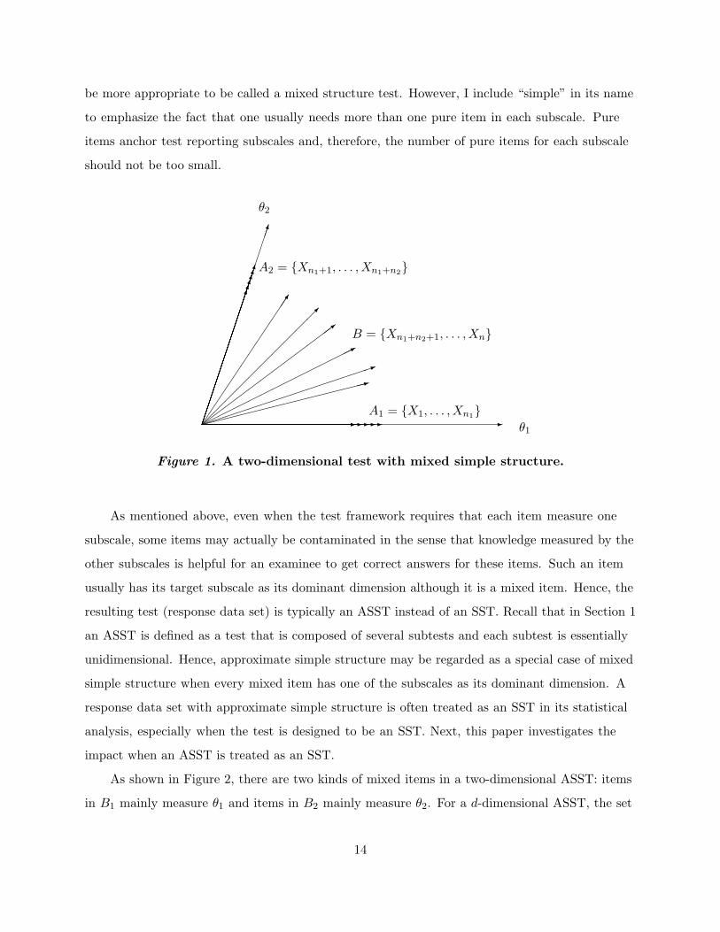
be more appropriate to be called a mixed structure test. However, I include “simple” in its name

to emphasize the fact that one usually needs more than one pure item in each subscale. Pure

items anchor test reporting subscales and, therefore, the number of pure items for each subscale

should not be too small.

-θ1

- -----A1 = {X1, . . . , Xn1}

��

θ2

��

��

��

��

��

��

A2 = {Xn1+1, . . . , Xn1+n2}

��:

��1

��

��

��*

��

��

��

��

��

��>

��

��

��

��

��

�

B = {Xn1+n2+1, . . . , Xn}

Figure 1. A two-dimensional test with mixed simple structure.

As mentioned above, even when the test framework requires that each item measure one

subscale, some items may actually be contaminated in the sense that knowledge measured by the

other subscales is helpful for an examinee to get correct answers for these items. Such an item

usually has its target subscale as its dominant dimension although it is a mixed item. Hence, the

resulting test (response data set) is typically an ASST instead of an SST. Recall that in Section 1

an ASST is defined as a test that is composed of several subtests and each subtest is essentially

unidimensional. Hence, approximate simple structure may be regarded as a special case of mixed

simple structure when every mixed item has one of the subscales as its dominant dimension. A

response data set with approximate simple structure is often treated as an SST in its statistical

analysis, especially when the test is designed to be an SST. Next, this paper investigates the

impact when an ASST is treated as an SST.

As shown in Figure 2, there are two kinds of mixed items in a two-dimensional ASST: items

in B1 mainly measure θ1 and items in B2 mainly measure θ2. For a d-dimensional ASST, the set

14

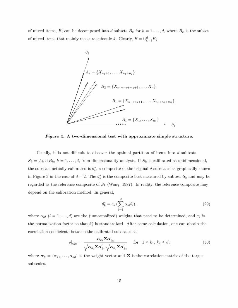
of mixed items, B, can be decomposed into d subsets Bk for k = 1, . . . , d, where Bk is the subset

of mixed items that mainly measure subscale k. Clearly, B = ∪dk=1Bk.

-θ1

- -----A1 = {X1, . . . , Xn1}

��

θ2

��

��

��

��

��

A2 = {Xn1+1, . . . , Xn1+n2}

��:

��:

��1

��1

B1 = {Xn1+n2+1, . . . , Xn1+n2+m1}

��

��

��

��

��7

�

��

�� B2 = {Xn1+n2+m1+1, . . . , Xn}

Figure 2. A two-dimensional test with approximate simple structure.

Usually, it is not difficult to discover the optimal partition of items into d subtests

Sk = Ak ∪ Bk, k = 1, . . . , d, from dimensionality analysis. If Sk is calibrated as unidimensional,

the subscale actually calibrated is θ∗k, a composite of the original d subscales as graphically shown

in Figure 3 in the case of d = 2. The θ∗k is the composite best measured by subtest Sk and may be

regarded as the reference composite of Sk (Wang, 1987). In reality, the reference composite may

depend on the calibration method. In general,

θ∗k = ck (d∑

l=1

αklθl), (29)

where αkl (l = 1, . . . , d) are the (unnormalized) weights that need to be determined, and ck is

the normalization factor so that θ∗k is standardized. After some calculation, one can obtain the

correlation coefficients between the calibrated subscales as

ρ∗k1k2=

αk1Σα′k2√

αk1Σα′k1

√αk2Σα

′k2

for 1 ≤ k1, k2 ≤ d, (30)

where αk = (αk1, . . . , αkd) is the weight vector and Σ is the correlation matrix of the target

subscales.

15

-θ1

- -----A1 = {X1, . . . , Xn1}

��

θ2

��

��

��

��

��

A2 = {Xn1+1, . . . , Xn1+n2}

��:

��:

��1

��1

B1 = {Xn1+n2+1, . . . , Xn1+n2+m1}

��

��

��

��

��7

�

��

�� B2 = {Xn1+n2+m1+1, . . . , Xn}

(((((((((((((((((((( θ∗1

��

θ∗2

Figure 3. The subscales calibrated are actually θ∗1 and θ∗2

when an ASST is treated as an SST.

Equation (30) gives the relationship between the correlation coefficients of the target subscales

and that of the calibrated subscales. Zhang and Stout (1999a) theoretically define a reference as

the composite at which the expected multidimensional critical ratio function achieves its maximum

value. According to Theorem 3 of Zhang and Stout (1999a), the weights of the composite are

mainly determined by the discrimination parameters. For subtest k (1 ≤ k ≤ d), an approximate

formula of weights is

αkl =∑i∈Sk

ail, l = 1, . . . , d.

Specifically,

αkk =∑i∈Ak

aik +∑i∈Bk

aik and αkl =∑i∈Bk

ail for l 6= k. (31)

Since Bk is the subset of items that mainly measure subscale k, aik > ail (l 6= k) for all items in

Bk. Hence, for any fixed k, αkk is always the largest weight among {αkl, l = 1, . . . , d}. In fact, αkk

is usually much larger than the others. Thus, the θ∗k in (29) is much closer to θk than the other θl

for l 6= k. Generally, all θ∗k should lie inside the convex region spanned by θk, k = 1, . . . , d, since all

weights are nonnegative. Hence, the correlation coefficients of θ∗k are larger than the corresponding

correlation coefficients of θk. Consequently, the correlation coefficients of the target subscales will

be overestimated since the correlation coefficients of θ∗k are actually estimated. The above results

16

are summarized in the theorem below.

Theorem 3. If an ASST is treated as an SST, the actually calibrated subscales are no

longer the target subscales though they could still be close to each other. The deviation between

a calibrated subscale and its corresponding target depends on how severe the subtest deviates

from unidimensionality. The correlation coefficients between calibrated subscales given by (30) are

larger than that between their respective target subscales.

Theorem 3 expresses the impact when an ASST is treated as an SST. Below an artificial

example is used to illustrate how large the difference is between the calibrated subscales’

correlation and the target subscales’ correlation.

Example 1. Suppose that all items in B1 measure the composite θ1 + 23θ2 in the sense that

the discrimination parameters of their secondary dimension (e.g., ai2) equal two thirds of the

discrimination parameters of their dominant dimension (e.g., ai1), and all items in B2 measure the

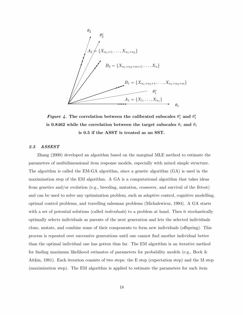
composite 23θ1 + θ2 as shown in Figure 4. If the magnitude of discrimination parameters and the

numbers of items in all subsets are balanced, then according to (29), θ∗1 should be in the middle

between A1 (i.e., θ1) and B1 (i.e., θ1 + 23θ2), and θ∗2 in the middle between A2 (i.e., θ2) and B2

(i.e., 23θ1 + θ2), that is,

θ∗1 = c1(θ1 +13θ2), and θ∗2 = c2(

13θ1 + θ2),

where c1 and c2 are the normalization constants. Let ρ be the correlation coefficient between

the original two subscales θ1 and θ2. Then, the correlation coefficient between θ∗1 and θ∗2 is

(6 + 10ρ)/(10 + 6ρ). If ρ is 0.5, then the correlation coefficient between θ∗1 and θ∗2 is 0.8462.

17

-θ1

----A1 = {X1, . . . , Xn1}

��

θ2

��

��

��

��

A2 = {Xn1+1, . . . , Xn1+n2}

��1

��1

��1

��1

B1 = {Xn1+n2+1, . . . , Xn1+n2+m}

(((((((((((((((((((( θ∗1

��

��

��

��

��

��7

��

��

��

��

��7

��

��

��

��

��7

��

��

��

��

��7B2 = {Xn1+n2+m+1, . . . , Xn}

��

θ∗2

Figure 4. The correlation between the calibrated subscales θ∗1 and θ∗1

is 0.8462 while the correlation between the target subscales θ1 and θ1

is 0.5 if the ASST is treated as an SST.

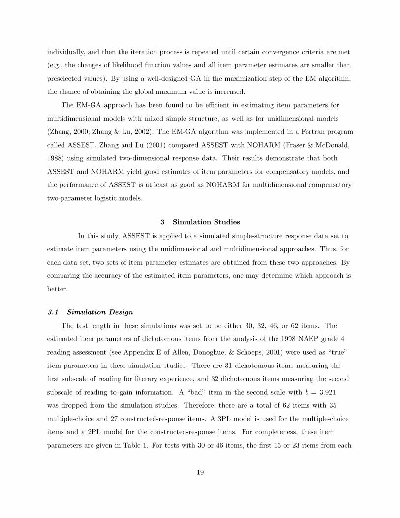
2.5 ASSEST

Zhang (2000) developed an algorithm based on the marginal MLE method to estimate the

parameters of multidimensional item response models, especially with mixed simple structure.

The algorithm is called the EM-GA algorithm, since a genetic algorithm (GA) is used in the

maximization step of the EM algorithm. A GA is a computational algorithm that takes ideas

from genetics and/or evolution (e.g., breeding, mutation, crossover, and survival of the fittest)

and can be used to solve any optimization problem, such as adaptive control, cognitive modelling,

optimal control problems, and travelling salesman problems (Michalewicsz, 1994). A GA starts

with a set of potential solutions (called individuals) to a problem at hand. Then it stochastically

optimally selects individuals as parents of the next generation and lets the selected individuals

clone, mutate, and combine some of their components to form new individuals (offspring). This

process is repeated over successive generations until one cannot find another individual better

than the optimal individual one has gotten thus far. The EM algorithm is an iterative method

for finding maximum likelihood estimates of parameters for probability models (e.g., Bock &

Aitkin, 1981). Each iteration consists of two steps: the E step (expectation step) and the M step

(maximization step). The EM algorithm is applied to estimate the parameters for each item

18

individually, and then the iteration process is repeated until certain convergence criteria are met

(e.g., the changes of likelihood function values and all item parameter estimates are smaller than

preselected values). By using a well-designed GA in the maximization step of the EM algorithm,

the chance of obtaining the global maximum value is increased.

The EM-GA approach has been found to be efficient in estimating item parameters for

multidimensional models with mixed simple structure, as well as for unidimensional models

(Zhang, 2000; Zhang & Lu, 2002). The EM-GA algorithm was implemented in a Fortran program

called ASSEST. Zhang and Lu (2001) compared ASSEST with NOHARM (Fraser & McDonald,

1988) using simulated two-dimensional response data. Their results demonstrate that both

ASSEST and NOHARM yield good estimates of item parameters for compensatory models, and

the performance of ASSEST is at least as good as NOHARM for multidimensional compensatory

two-parameter logistic models.

3 Simulation Studies

In this study, ASSEST is applied to a simulated simple-structure response data set to

estimate item parameters using the unidimensional and multidimensional approaches. Thus, for

each data set, two sets of item parameter estimates are obtained from these two approaches. By

comparing the accuracy of the estimated item parameters, one may determine which approach is

better.

3.1 Simulation Design

The test length in these simulations was set to be either 30, 32, 46, or 62 items. The

estimated item parameters of dichotomous items from the analysis of the 1998 NAEP grade 4

reading assessment (see Appendix E of Allen, Donoghue, & Schoeps, 2001) were used as “true”

item parameters in these simulation studies. There are 31 dichotomous items measuring the

first subscale of reading for literary experience, and 32 dichotomous items measuring the second

subscale of reading to gain information. A “bad” item in the second scale with b = 3.921

was dropped from the simulation studies. Therefore, there are a total of 62 items with 35

multiple-choice and 27 constructed-response items. A 3PL model is used for the multiple-choice

items and a 2PL model for the constructed-response items. For completeness, these item

parameters are given in Table 1. For tests with 30 or 46 items, the first 15 or 23 items from each

19

scale were chosen. For instance, the items in the 30-item test are items 1-15 and items 32-46 in

Table 1. The 32-item test consists of the remaining items after the 30-item test was selected from

the total 62 items. That is, the 32-item test is the complement of the 30-item test and consists of

items 16-31 and 47-62. The purpose of including this complement test in the simulation study is

to check whether different sets of item parameters have impact on the estimation results. In short,

there are two sets of embedded tests (i.e., a shorter test is a part of a longer test) in this simulation

design: the set of the 30-, 46-, and 62-item tests and the set of the 32- and 62-item tests.

The number of simulated examinees was 500, 1,000, 2,000, 3,000, 4,000, or 5,000 in this

study. Examinees’ (true) ability scores were generated independently from a bivariate normal

distribution with means of 0, variances of 1, and a (population) correlation of 0.0, 0.5, or 0.8. Not

that the estimated correlation coefficients between subscales in NAEP assessments are usually

around 0.8 (see Allen, Donoghue, & Schoeps, 2001), and the typical correlation coefficient is 0.5

between math and verbal in an achievement test with math and verbal sections, such as the SAT.

From the last section, when the correlation coefficient is zero, theoretically, there should be no

difference between the unidimensional and multidimensional approaches. Any difference between

the unidimensional and multidimensional approaches when the correlation coefficient is zero is

caused by numerical rounding error in ASSEST, which provides a reference when comparing

differences in other cases. Of course, the multidimensional approach has additional errors from

estimation of the correlation. However, the impact should be small, if it is not negligible, since the

errors from estimation of the correlation are typically small.

Simulated response data were generated using the following (standard) IRT method. Given

ability score θj , first calculate the probability of answering item i correctly by examinee j,

pij = Pi(θj), using item parameters from Table 1. Then generate a random number r from the

(0, 1) uniform distribution. If r < pij , then a correct response was obtained for examinee j on

item i; otherwise, an incorrect response was obtained. It should be noted that in this simulation

study a smaller data set is always just a part of its corresponding larger data set. For example, a

30-item response data set is a part of a 62-item response data set at the same level of correlation.

In this way, sampling variations may be reduced.

20

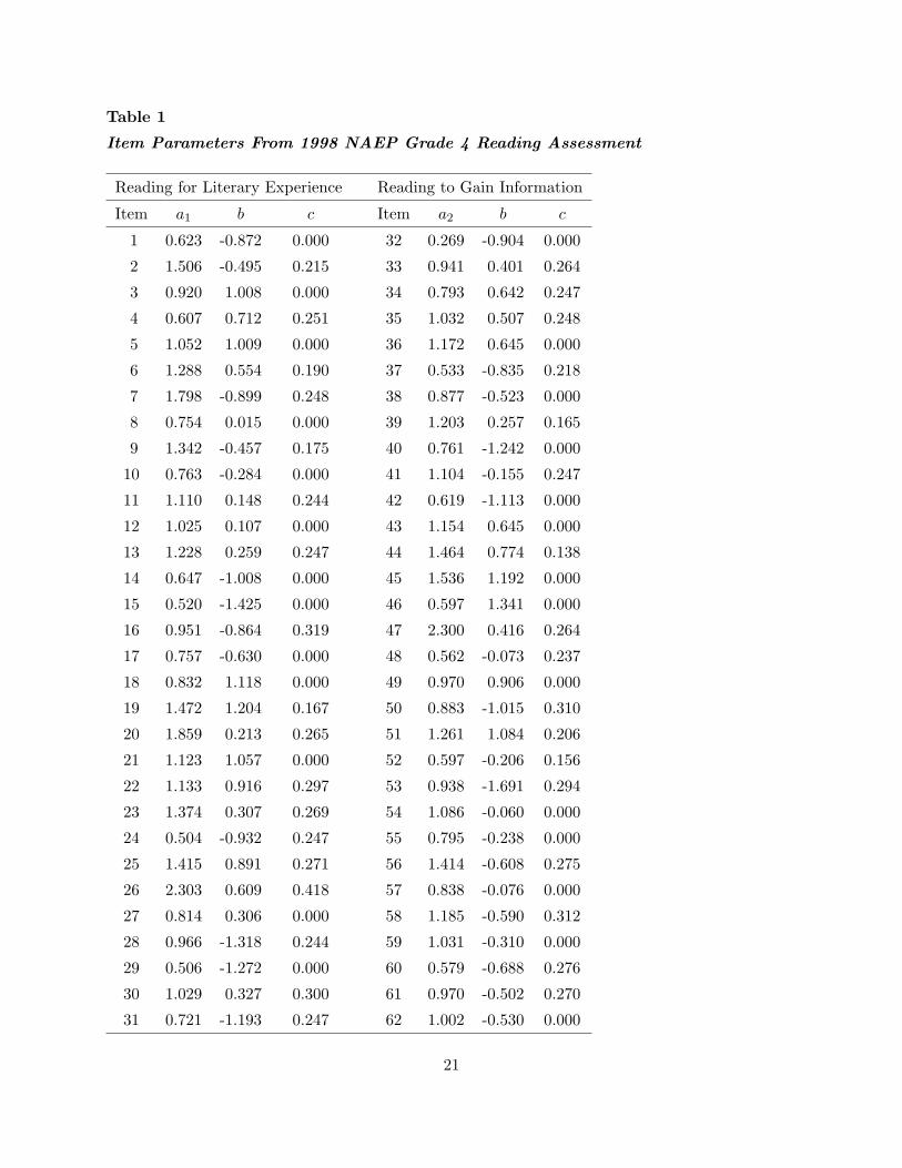
Table 1

Item Parameters From 1998 NAEP Grade 4 Reading Assessment

Reading for Literary Experience Reading to Gain Information

Item a1 b c Item a2 b c

1 0.623 -0.872 0.000 32 0.269 -0.904 0.000

2 1.506 -0.495 0.215 33 0.941 0.401 0.264

3 0.920 1.008 0.000 34 0.793 0.642 0.247

4 0.607 0.712 0.251 35 1.032 0.507 0.248

5 1.052 1.009 0.000 36 1.172 0.645 0.000

6 1.288 0.554 0.190 37 0.533 -0.835 0.218

7 1.798 -0.899 0.248 38 0.877 -0.523 0.000

8 0.754 0.015 0.000 39 1.203 0.257 0.165

9 1.342 -0.457 0.175 40 0.761 -1.242 0.000

10 0.763 -0.284 0.000 41 1.104 -0.155 0.247

11 1.110 0.148 0.244 42 0.619 -1.113 0.000

12 1.025 0.107 0.000 43 1.154 0.645 0.000

13 1.228 0.259 0.247 44 1.464 0.774 0.138

14 0.647 -1.008 0.000 45 1.536 1.192 0.000

15 0.520 -1.425 0.000 46 0.597 1.341 0.000

16 0.951 -0.864 0.319 47 2.300 0.416 0.264

17 0.757 -0.630 0.000 48 0.562 -0.073 0.237

18 0.832 1.118 0.000 49 0.970 0.906 0.000

19 1.472 1.204 0.167 50 0.883 -1.015 0.310

20 1.859 0.213 0.265 51 1.261 1.084 0.206

21 1.123 1.057 0.000 52 0.597 -0.206 0.156

22 1.133 0.916 0.297 53 0.938 -1.691 0.294

23 1.374 0.307 0.269 54 1.086 -0.060 0.000

24 0.504 -0.932 0.247 55 0.795 -0.238 0.000

25 1.415 0.891 0.271 56 1.414 -0.608 0.275

26 2.303 0.609 0.418 57 0.838 -0.076 0.000

27 0.814 0.306 0.000 58 1.185 -0.590 0.312

28 0.966 -1.318 0.244 59 1.031 -0.310 0.000

29 0.506 -1.272 0.000 60 0.579 -0.688 0.276

30 1.029 0.327 0.300 61 0.970 -0.502 0.270

31 0.721 -1.193 0.247 62 1.002 -0.530 0.000

21

In summary, this simulation study considers the following three factors:

1. the number of items: 30, 32, 46, or 62;

2. the number of simulated examinees: 500, 1,000, 2,000, 3,000, 4,000, or 5,000; and

3. the correlation coefficient between two subscales: 0.0, 0.5, or 0.8.

Given these factors, there were 72 combinations in this simulation. For each combination,

ASSEST was applied to a simulated response data set twice to get two sets of parameter estimates

under two different specifications, corresponding to the unidimensional and multidimensional

approaches. This process was repeated 100 times for each combination.

3.2 Criterion for Comparisons

In this simulation study, two different kinds of root mean-squared error (RMSE) were

calculated as comparison criterions. The first kind focuses on the recovery of item parameters and

the second kind on the recovery of IRFs directly.

The RMSE of estimated parameters is commonly used as a criterion for the recovery of item

parameters in simulation studies. The RMSE is the square root of the average of the squared

deviations of estimated parameters from the corresponding true ones. Let γi represent a parameter

of item i, ai1, ai2, bi, or ci, and γ̂ij be the estimate of γi from the jth replications for i = 1, . . . , n

and j = 1, . . . , J . Here n is the number of items and J is the number of replications (J = 100 in

the simulation studies). For each item parameter, define

RMSE(γi) =

√√√√ 1J

J∑j=1

(γ̂ij − γi)2.

Given an SST with n items, the total number of item parameters is 2n (n discrimination and n

difficulty parameters) plus the number of lower-asymptote parameters (i.e., the number of items

in the test modelled by the M3PL model). So is the number of RMSEs. To make the comparison

feasible, these RMSEs are further summarized by types of item parameters. If the test has two

subtests, then there are four types of item parameters, the discrimination parameter for the first

subscale a1, the discrimination parameter for the second subscale a2, the difficulty parameter b,

and the lower-asymptote parameter c for multiple-choice items. To further summarize the RMSE,

22

the average of the RMSEs, ARMSE, for each of these four kinds of item parameters is defined as

ARMSE(γ) =1

#Sγ

∑i∈Sγ

RMSR(γi) =1

#Sγ

∑i∈Sγ

√√√√ 1J

J∑j=1

(γ̂ij − γi)2, (32)

where γ represents one of the four kinds of item parameters, Sγ is the set of item sequence numbers

that have γ parameter and #Sγ is the number of elements in Sγ . If γ is the discrimination

parameter of the second subscale, for example, then Sa2 = {n1 + 1, n1 + 2, . . . , n} and #Sa2 = n2.

If γ is the lower-asymptote parameter, then Sc = {i: item i is a multiple-choice item, 1 ≤ i ≤ n}

and #Sc is the number of items modelled by M3PL models. For each of the two different

dimensional estimation approaches, there are four ARMSE(γ) for each of the 72 combinations

considered in the simulation study. These values (total of 2× 4× 72 = 576) together with ARMSE

of estimated IRF defined later are reported in Tables 2-4, which will be discussed later.

The estimates of item parameters are usually treated as fixed in any further analysis of

response data such as estimating abilities of examinees. In the process of such analysis, the IRF

is more directly relevant than item parameters themselves in operational applications since most

statistical analysis is based on the likelihood function formed by the IRFs. In addition, different

sets of item parameters may produce very close item characteristic curves or surfaces. Therefore,

it is more appropriate and vital to check the closeness of estimated IRF (curves or surfaces) to

the true IRF than the item parameter estimates to the true values. Moreover, it is possible when

making comparisons using the ARMSE of estimated parameters, one approach is better than

the other for some parameters (e.g., discrimination parameters), but worse for other parameters

(e.g., the lower-asymptote parameter). This did happen in the simulation study, for instance, in

the cases of 62 items with 0.8 correlation (see Table 4). Hence it is necessary to directly use the

RMSE for the estimated IRF. Let P̂ij(θ) be the estimated IRF of true IRF Pi(θ) from the jth

replication. The RMSE of P̂ij(θ) is defined as

dij =√

E{[P̂ij(Ξ)− Pi(Ξ)]2},

where the expectation E is respect to the latent ability vector Ξ. Or

dij =

√∫[P̂ij(θ)− Pi(θ)]2ϕ(θ | Σ)dθ, (33)

where ϕ(θ | Σ) is the density function of the latent ability vector and Σ is its correlation matrix.

The RMSE of an estimated IRF is its Euclidean distance from its corresponding true IRF.

23

Clearly, the smaller the RMSE, the better the estimator is. This simulation study considers only

two-dimensional tests, and the density function of the latent ability vector is given by (11). From

(33), the RMSE of an estimated IRF is

dij =

√∫ ∫[P̂ij(θ1, θ2)− Pi(θ1, θ2)]2ϕ(θ1, θ2 | ρ)dθ1dθ2, (34)

where ϕ(θ1, θ2 | ρ) is given by (11). When the test has a simple structure, (34) can be simplified as

dij =

√∫[P̂ij(θ)− Pi(θ)]2ϕ(θ)dθ, (35)

where Pi(θ) is given by either (3) when the item measures the first subscale or (4) when it

measures the second subscale, and ϕ(θ) is the marginal density function of ϕ(θ1, θ2 | ρ), which

is the standard normal distribution in this case here. Note that this paper does not distinguish

between θ1 and θ2 in (35) since they are just integral (dummy) variables.

The RMSEs of different IRFs in the same test may be quite different from each other because

of different item characteristics. The average of the RMSEs among the items in a test across

all replications will be used as an overall measure of the accuracy of the estimation, that is the

overall average d̄ = 1nJ

∑ni=1

∑Jj=1 dij , called the ARMSE of estimated IRF. For each of the 72

combinations considered in this study, two ARMSE were calculated based on the estimated IRF

from the unidimensional and multidimensional approaches, respectively, and are reported in the

last columns in Tables 2-4.

The RMSE of estimated item parameters is on the same scale as the item parameter.

However, the magnitude of the RMSE of an estimated IRF has no clear absolute reference

although it is always between zero and one. This study, however, is mainly interested in the

relative values of ARMSE between the unidimensional and multidimensional approaches, not in

their magnitudes. Nevertheless, these RMSEs of estimated item parameters and IRFs are together

in Tables 2-4 to give a reference for the scale of RMSE of an estimated IRF relative to that of the

RMSE of estimated item parameters.

24

Table 2

ARMSE of Estimated Item Parameters and IRF When Correlation Between

Subscales Is 0.0

Number of Number a1 a2 b c IRF

Examinees of Items

500 30 0.2312, 0.2336 0.2344, 0.2329 0.1847, 0.1849 0.0983, 0.0983 0.0321, 0.0321

32 0.2955, 0.2946 0.2377, 0.2391 0.2352, 0.2336 0.1154, 0.1146 0.0333, 0.0331

46 0.2473, 0.2474 0.2201, 0.2203 0.1920, 0.1917 0.0961, 0.0965 0.0319, 0.0319

62 0.2458, 0.2459 0.2108, 0.2112 0.1916, 0.1921 0.1010, 0.1011 0.0299, 0.0299

1,000 30 0.1588, 0.1603 0.1554, 0.1539 0.1393, 0.1387 0.0774, 0.0766 0.0231, 0.0231

32 0.2138, 0.2140 0.1736, 0.1744 0.1887, 0.1884 0.0988, 0.0976 0.0244, 0.0244

46 0.1657, 0.1642 0.1525, 0.1537 0.1493, 0.1496 0.0761, 0.0765 0.0238, 0.0238

62 0.1704, 0.1703 0.1502, 0.1500 0.1495, 0.1491 0.0825, 0.0817 0.0216, 0.0216

2,000 30 0.1123, 0.1108 0.1045, 0.1049 0.1047, 0.1052 0.0578, 0.0576 0.0170, 0.0171

32 0.1592, 0.1599 0.1255, 0.1257 0.1497, 0.1500 0.0782, 0.0778 0.0180, 0.0180

46 0.1176, 0.1171 0.1073, 0.1080 0.1175, 0.1184 0.0584, 0.0592 0.0182, 0.0184

62 0.1241, 0.1250 0.1080, 0.1084 0.1151, 0.1153 0.0639, 0.0635 0.0158, 0.0158

3,000 30 0.0952, 0.0934 0.0879, 0.0886 0.0918, 0.0907 0.0494, 0.0485 0.0148, 0.0147

32 0.1287, 0.1288 0.1067, 0.1046 0.1330, 0.1348 0.0674, 0.0682 0.0157, 0.0156

46 0.0987, 0.0975 0.0917, 0.0917 0.1043, 0.1047 0.0499, 0.0502 0.0162, 0.0163

62 0.1045, 0.1037 0.0924, 0.0919 0.1005, 0.0998 0.0545, 0.0540 0.0135, 0.0135

4,000 30 0.0848, 0.0849 0.0762, 0.0771 0.0826, 0.0832 0.0439, 0.0444 0.0131, 0.0133

32 0.1149, 0.1152 0.0942, 0.0933 0.1244, 0.1238 0.0632, 0.0624 0.0141, 0.0140

46 0.0849, 0.0837 0.0807, 0.0809 0.0953, 0.0954 0.0448, 0.0452 0.0149, 0.0150

62 0.0920, 0.0913 0.0828, 0.0822 0.0905, 0.0906 0.0487, 0.0488 0.0120, 0.0119

5,000 30 0.0742, 0.0755 0.0678, 0.0683 0.0769, 0.0769 0.0404, 0.0404 0.0121, 0.0123

32 0.1027, 0.1037 0.0862, 0.0859 0.1168, 0.1168 0.0580, 0.0577 0.0131, 0.0131

46 0.0739, 0.0734 0.0729, 0.0716 0.0892, 0.0882 0.0405, 0.0408 0.0140, 0.0137

62 0.0831, 0.0821 0.0761, 0.0751 0.0855, 0.0840 0.0456, 0.0448 0.0111, 0.0109

Note. Based on 100 replications using unidimensional and multidimensional approaches. The two

numbers in each cell in columns 3-7 are the ARMSEs from the unidimensional and

multidimensional approaches, respectively.

25

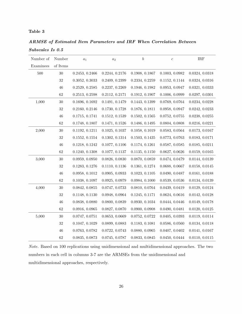
Table 3


Subscales Is 0.5


Examinees of Items

500 30 0.2453, 0.2466 0.2244, 0.2176 0.1908, 0.1867 0.1003, 0.0982 0.0324, 0.0318

32 0.3052, 0.3033 0.2409, 0.2399 0.2334, 0.2259 0.1152, 0.1144 0.0324, 0.0316

46 0.2529, 0.2585 0.2237, 0.2269 0.1946, 0.1982 0.0953, 0.0947 0.0321, 0.0333

62 0.2513, 0.2598 0.2112, 0.2171 0.1912, 0.1907 0.1006, 0.0999 0.0297, 0.0301

1,000 30 0.1696, 0.1692 0.1491, 0.1479 0.1443, 0.1399 0.0769, 0.0764 0.0234, 0.0228

32 0.2160, 0.2146 0.1730, 0.1728 0.1876, 0.1811 0.0958, 0.0947 0.0242, 0.0233

46 0.1715, 0.1741 0.1512, 0.1539 0.1502, 0.1565 0.0752, 0.0755 0.0238, 0.0255

62 0.1748, 0.1807 0.1471, 0.1526 0.1486, 0.1495 0.0804, 0.0808 0.0216, 0.0221

2,000 30 0.1192, 0.1211 0.1025, 0.1037 0.1058, 0.1019 0.0583, 0.0564 0.0173, 0.0167

32 0.1552, 0.1554 0.1302, 0.1314 0.1503, 0.1435 0.0773, 0.0763 0.0183, 0.0171

46 0.1218, 0.1242 0.1077, 0.1106 0.1174, 0.1261 0.0587, 0.0585 0.0185, 0.0211

62 0.1240, 0.1308 0.1077, 0.1137 0.1135, 0.1150 0.0627, 0.0626 0.0159, 0.0165

3,000 30 0.0959, 0.0950 0.0826, 0.0830 0.0870, 0.0859 0.0474, 0.0479 0.0144, 0.0139

32 0.1283, 0.1276 0.1110, 0.1136 0.1361, 0.1274 0.0688, 0.0667 0.0158, 0.0145

46 0.0958, 0.1012 0.0905, 0.0933 0.1023, 0.1105 0.0490, 0.0487 0.0161, 0.0188

62 0.1038, 0.1097 0.0925, 0.0979 0.0984, 0.1000 0.0539, 0.0536 0.0134, 0.0139

4,000 30 0.0842, 0.0855 0.0747, 0.0733 0.0810, 0.0764 0.0439, 0.0419 0.0129, 0.0124

32 0.1148, 0.1130 0.0948, 0.0964 0.1245, 0.1171 0.0624, 0.0616 0.0142, 0.0128

46 0.0838, 0.0880 0.0800, 0.0839 0.0930, 0.1034 0.0444, 0.0446 0.0149, 0.0178

62 0.0916, 0.0965 0.0827, 0.0870 0.0900, 0.0908 0.0490, 0.0481 0.0120, 0.0125

5,000 30 0.0747, 0.0751 0.0653, 0.0669 0.0752, 0.0722 0.0405, 0.0393 0.0119, 0.0114

32 0.1047, 0.1029 0.0899, 0.0883 0.1183, 0.1081 0.0586, 0.0560 0.0134, 0.0118

46 0.0763, 0.0782 0.0722, 0.0743 0.0880, 0.0965 0.0407, 0.0402 0.0141, 0.0167

62 0.0835, 0.0873 0.0745, 0.0787 0.0833, 0.0845 0.0450, 0.0444 0.0110, 0.0115




26

Table 4


Subscales Is 0.8


Examinees of Items

500 30 0.2309, 0.2239 0.2180, 0.2080 0.1840, 0.1785 0.1009, 0.0962 0.0318, 0.0306

32 0.3112, 0.3004 0.2460, 0.2328 0.2282, 0.2196 0.1121, 0.1102 0.0324, 0.0311

46 0.2459, 0.2449 0.2207, 0.2220 0.1914, 0.1955 0.0976, 0.0944 0.0315, 0.0332

62 0.2499, 0.2547 0.2095, 0.2174 0.1919, 0.1881 0.1013, 0.0987 0.0296, 0.0302

1,000 30 0.1618, 0.1593 0.1469, 0.1407 0.1401, 0.1335 0.0772, 0.0730 0.0233, 0.0223

32 0.2186, 0.2035 0.1752, 0.1660 0.1857, 0.1729 0.0956, 0.0915 0.0241, 0.0225

46 0.1728, 0.1763 0.1534, 0.1563 0.1498, 0.1584 0.0759, 0.0744 0.0237, 0.0266

62 0.1745, 0.1851 0.1488, 0.1588 0.1470, 0.1465 0.0799, 0.0783 0.0215, 0.0226

2,000 30 0.1124, 0.1095 0.0999, 0.1001 0.1072, 0.1006 0.0582, 0.0547 0.0171, 0.0165

32 0.1558, 0.1465 0.1261, 0.1216 0.1498, 0.1404 0.0766, 0.0748 0.0180, 0.0164

46 0.1143, 0.1216 0.1074, 0.1128 0.1160, 0.1278 0.0584, 0.0563 0.0180, 0.0222

62 0.1225, 0.1355 0.1073, 0.1198 0.1139, 0.1160 0.0623, 0.0603 0.0157, 0.0172

3,000 30 0.0902, 0.0886 0.0831, 0.0811 0.0884, 0.0832 0.0470, 0.0436 0.0144, 0.0139

32 0.1281, 0.1179 0.1068, 0.1026 0.1324, 0.1211 0.0663, 0.0646 0.0155, 0.0137

46 0.0953, 0.1004 0.0899, 0.0960 0.1022, 0.1160 0.0493, 0.0474 0.0159, 0.0204

62 0.1003, 0.1129 0.0898, 0.1028 0.0991, 0.1019 0.0540, 0.0523 0.0132, 0.0148

4,000 30 0.0774, 0.0790 0.0727, 0.0722 0.0800, 0.0769 0.0415, 0.0404 0.0129, 0.0126

32 0.1184, 0.1093 0.0943, 0.0895 0.1244, 0.1133 0.0622, 0.0599 0.0142, 0.0125

46 0.0836, 0.0901 0.0783, 0.0846 0.0932, 0.1056 0.0442, 0.0424 0.0147, 0.0191

62 0.0900, 0.1011 0.0808, 0.0915 0.0898, 0.0929 0.0486, 0.0470 0.0120, 0.0134

5,000 30 0.0727, 0.0744 0.0677, 0.0658 0.0740, 0.0700 0.0391, 0.0367 0.0119, 0.0115

32 0.1053, 0.0976 0.0864, 0.0826 0.1168, 0.1050 0.0577, 0.0547 0.0132, 0.0113

46 0.0761, 0.0811 0.0717, 0.0762 0.0870, 0.0982 0.0402, 0.0380 0.0138, 0.0178

62 0.0828, 0.0905 0.0734, 0.0819 0.0828, 0.0848 0.0445, 0.0426 0.0109, 0.0120




27

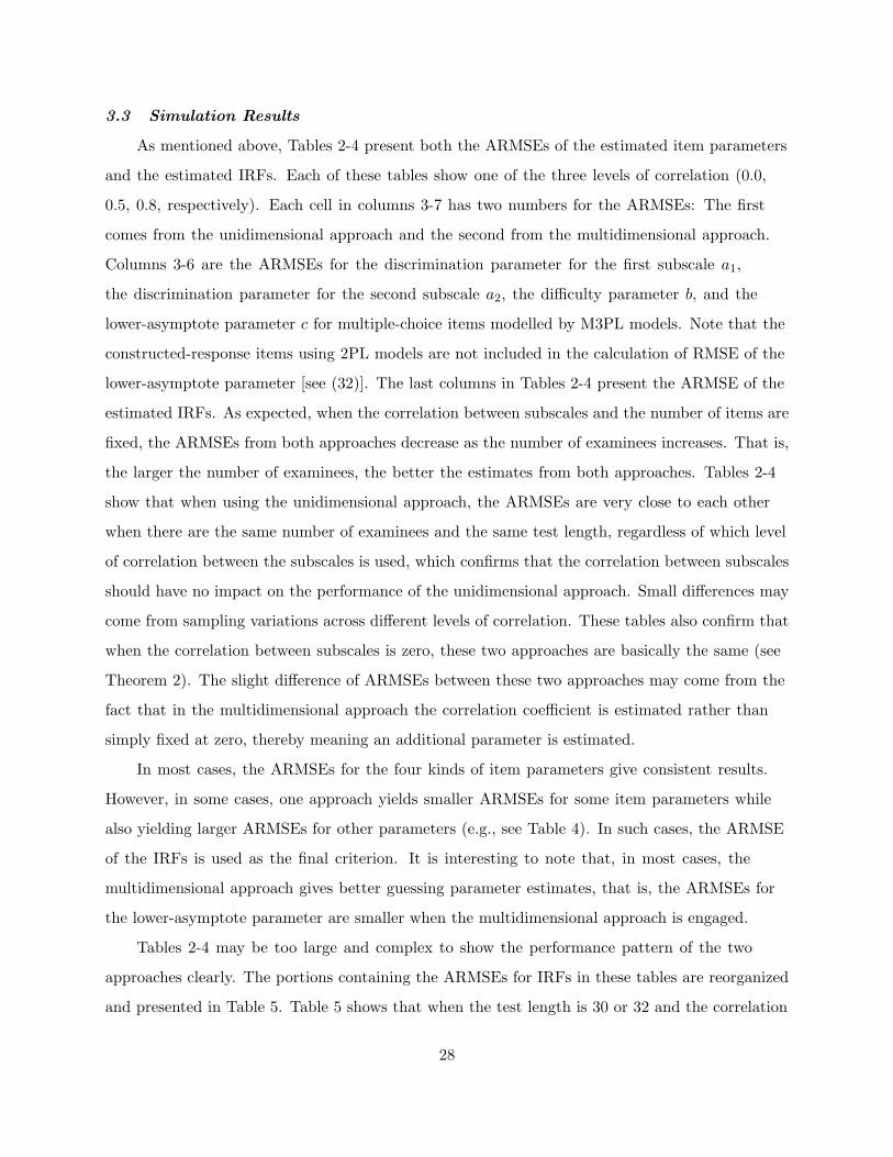
3.3 Simulation Results

As mentioned above, Tables 2-4 present both the ARMSEs of the estimated item parameters

and the estimated IRFs. Each of these tables show one of the three levels of correlation (0.0,

0.5, 0.8, respectively). Each cell in columns 3-7 has two numbers for the ARMSEs: The first

comes from the unidimensional approach and the second from the multidimensional approach.

Columns 3-6 are the ARMSEs for the discrimination parameter for the first subscale a1,

the discrimination parameter for the second subscale a2, the difficulty parameter b, and the

lower-asymptote parameter c for multiple-choice items modelled by M3PL models. Note that the

constructed-response items using 2PL models are not included in the calculation of RMSE of the

lower-asymptote parameter [see (32)]. The last columns in Tables 2-4 present the ARMSE of the

estimated IRFs. As expected, when the correlation between subscales and the number of items are

fixed, the ARMSEs from both approaches decrease as the number of examinees increases. That is,

the larger the number of examinees, the better the estimates from both approaches. Tables 2-4

show that when using the unidimensional approach, the ARMSEs are very close to each other

when there are the same number of examinees and the same test length, regardless of which level

of correlation between the subscales is used, which confirms that the correlation between subscales

should have no impact on the performance of the unidimensional approach. Small differences may

come from sampling variations across different levels of correlation. These tables also confirm that

when the correlation between subscales is zero, these two approaches are basically the same (see

Theorem 2). The slight difference of ARMSEs between these two approaches may come from the

fact that in the multidimensional approach the correlation coefficient is estimated rather than

simply fixed at zero, thereby meaning an additional parameter is estimated.

In most cases, the ARMSEs for the four kinds of item parameters give consistent results.

However, in some cases, one approach yields smaller ARMSEs for some item parameters while

also yielding larger ARMSEs for other parameters (e.g., see Table 4). In such cases, the ARMSE

of the IRFs is used as the final criterion. It is interesting to note that, in most cases, the

multidimensional approach gives better guessing parameter estimates, that is, the ARMSEs for

the lower-asymptote parameter are smaller when the multidimensional approach is engaged.

Tables 2-4 may be too large and complex to show the performance pattern of the two

approaches clearly. The portions containing the ARMSEs for IRFs in these tables are reorganized

and presented in Table 5. Table 5 shows that when the test length is 30 or 32 and the correlation

28

is either 0.5 or 0.8, the average of the ARMSEs from the multidimensional approach is uniformly

smaller than the corresponding average of the ARMSEs from the unidimensional approach across

all numbers of examinees considered here. In contrast, when the test length is increased to 46 or

62, while the correlation still remains 0.5 or 0.8, the unidimensional approach is uniformly better

(with smaller ARMSEs) than the multidimensional approach across all numbers of examinees.

These results suggest that when the test length is relatively short, the additional information

from other subscales’ items is helpful in obtaining more accurate IRF estimates if these scales are

positively correlated. Otherwise, the additional information from other subscales may not be as

helpful, but may even be harmful to the accuracy of parameter/IRF estimations, since additional

statistical and numerical noises are also likely introduced when employing the multidimensional

approach.

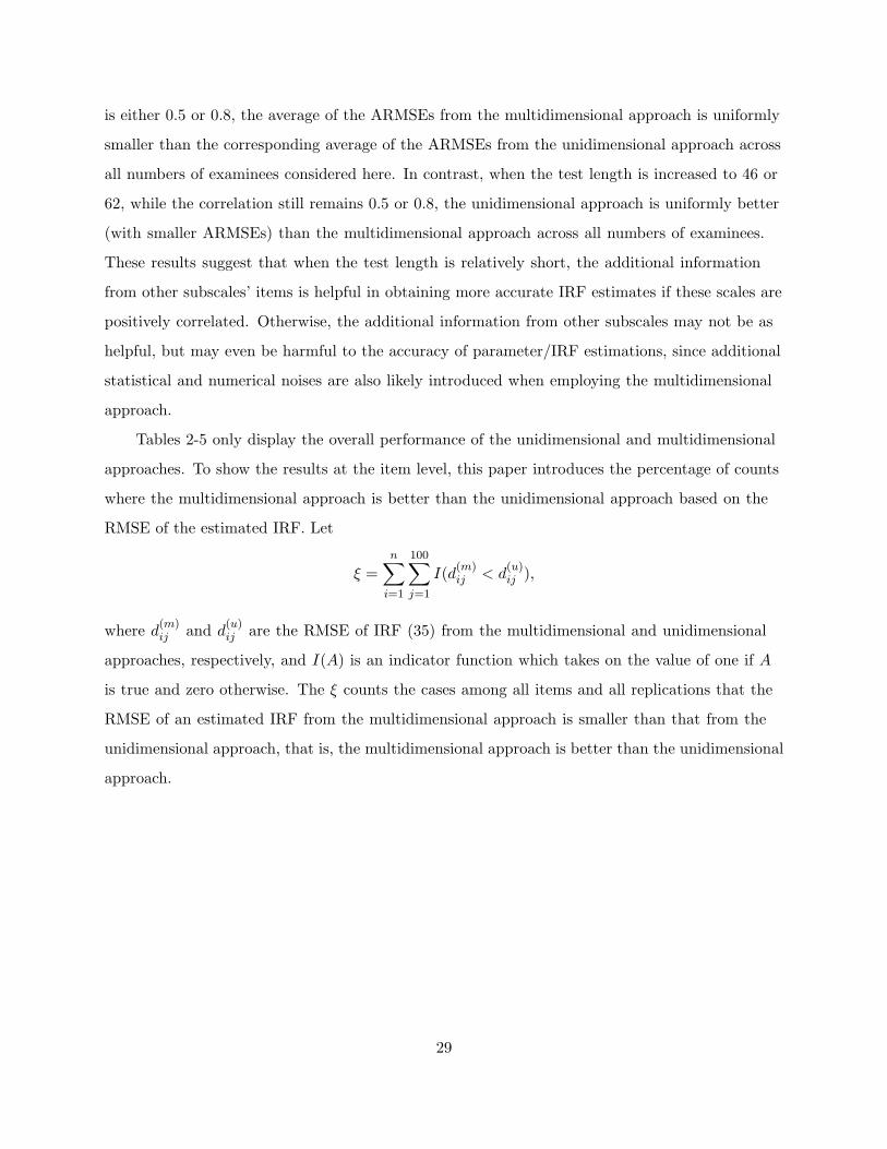
Tables 2-5 only display the overall performance of the unidimensional and multidimensional

approaches. To show the results at the item level, this paper introduces the percentage of counts

where the multidimensional approach is better than the unidimensional approach based on the

RMSE of the estimated IRF. Let

ξ =n∑

i=1

100∑j=1

I(d(m)ij < d

(u)ij ),

where d(m)ij and d

(u)ij are the RMSE of IRF (35) from the multidimensional and unidimensional

approaches, respectively, and I(A) is an indicator function which takes on the value of one if A

is true and zero otherwise. The ξ counts the cases among all items and all replications that the

RMSE of an estimated IRF from the multidimensional approach is smaller than that from the

unidimensional approach, that is, the multidimensional approach is better than the unidimensional

approach.

29

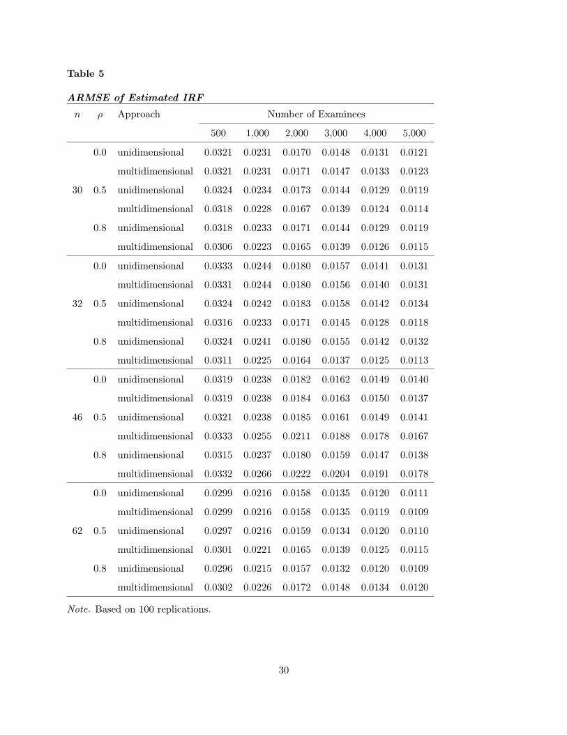
Table 5

ARMSE of Estimated IRF

n ρ Approach Number of Examinees

500 1,000 2,000 3,000 4,000 5,000

0.0 unidimensional 0.0321 0.0231 0.0170 0.0148 0.0131 0.0121

multidimensional 0.0321 0.0231 0.0171 0.0147 0.0133 0.0123

30 0.5 unidimensional 0.0324 0.0234 0.0173 0.0144 0.0129 0.0119


0.8 unidimensional 0.0318 0.0233 0.0171 0.0144 0.0129 0.0119


0.0 unidimensional 0.0333 0.0244 0.0180 0.0157 0.0141 0.0131


32 0.5 unidimensional 0.0324 0.0242 0.0183 0.0158 0.0142 0.0134


0.8 unidimensional 0.0324 0.0241 0.0180 0.0155 0.0142 0.0132


0.0 unidimensional 0.0319 0.0238 0.0182 0.0162 0.0149 0.0140


46 0.5 unidimensional 0.0321 0.0238 0.0185 0.0161 0.0149 0.0141


0.8 unidimensional 0.0315 0.0237 0.0180 0.0159 0.0147 0.0138


0.0 unidimensional 0.0299 0.0216 0.0158 0.0135 0.0120 0.0111


62 0.5 unidimensional 0.0297 0.0216 0.0159 0.0134 0.0120 0.0110


0.8 unidimensional 0.0296 0.0215 0.0157 0.0132 0.0120 0.0109


Note. Based on 100 replications.

30

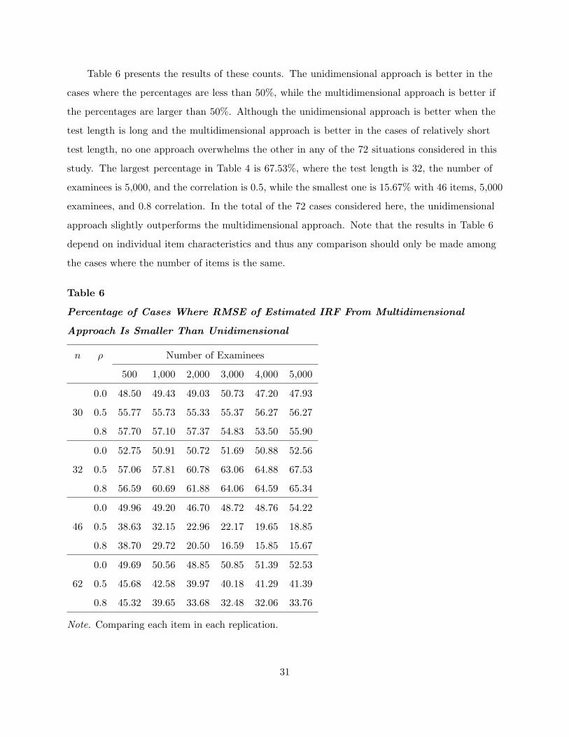
Table 6 presents the results of these counts. The unidimensional approach is better in the

cases where the percentages are less than 50%, while the multidimensional approach is better if

the percentages are larger than 50%. Although the unidimensional approach is better when the

test length is long and the multidimensional approach is better in the cases of relatively short

test length, no one approach overwhelms the other in any of the 72 situations considered in this

study. The largest percentage in Table 4 is 67.53%, where the test length is 32, the number of

examinees is 5,000, and the correlation is 0.5, while the smallest one is 15.67% with 46 items, 5,000

examinees, and 0.8 correlation. In the total of the 72 cases considered here, the unidimensional

approach slightly outperforms the multidimensional approach. Note that the results in Table 6

depend on individual item characteristics and thus any comparison should only be made among

the cases where the number of items is the same.

Table 6

Percentage of Cases Where RMSE of Estimated IRF From Multidimensional

Approach Is Smaller Than Unidimensional

n ρ Number of Examinees

500 1,000 2,000 3,000 4,000 5,000

0.0 48.50 49.43 49.03 50.73 47.20 47.93

30 0.5 55.77 55.73 55.33 55.37 56.27 56.27

0.8 57.70 57.10 57.37 54.83 53.50 55.90

0.0 52.75 50.91 50.72 51.69 50.88 52.56

32 0.5 57.06 57.81 60.78 63.06 64.88 67.53

0.8 56.59 60.69 61.88 64.06 64.59 65.34

0.0 49.96 49.20 46.70 48.72 48.76 54.22

46 0.5 38.63 32.15 22.96 22.17 19.65 18.85

0.8 38.70 29.72 20.50 16.59 15.85 15.67

0.0 49.69 50.56 48.85 50.85 51.39 52.53

62 0.5 45.68 42.58 39.97 40.18 41.29 41.39

0.8 45.32 39.65 33.68 32.48 32.06 33.76

Note. Comparing each item in each replication.

31

When using the multidimensional approach, the estimates of correlation coefficients between

abilities are also obtained as a by-product. These estimates are pretty close to their corresponding

true correlations. Table 7 presents the RMSE of estimated correlations, which is the square root

of the average of the squared deviations of estimated correlations from their corresponding true

correlation based on 100 replications. As shown in Table 7, the largest RMSE is 0.0380, which

appears in the 30-item 500-examinee zero-correlation case, while the smallest RMSE is 0.0084 in

the case of 30 items, 5,000 examinees, and 0.8 correlation. Generally speaking, the greater the

number of examinees, the better the estimated correlation is. However, the impact of test length

and the correlation between scales on the estimation of the correlation is not so straightforward. It

seems that some interactions exist among these three factors. For example, when the test length

is 30 or 32, for any fixed number of examinees, the RMSE decreases as the correlation increases.

But when the number of item is 62, this pattern holds only in the case of 500 examinees (see

Table 7). In uncorrelated cases (ρ = 0.0), with any fixed number of examinees, the RMSE for

embedded tests (e.g., 30-, 46-, and 62-item tests) decreases as the number of items increases. In

contrast, when the correlation is either 0.5 or 0.8, the RMSE increases as the number of items

increases except for the cases of 500 (with ρ = 0.5 or 0.8) or 1,000 (with ρ = 0.5 only) examinees

for the tests of 30, 46, and 62 items as shown in Table 7. Here this paper focuses on the embedded

tests to control the impact of item parameters (item quality) on the estimation. Note that in

practice, scales to be measured by a test are usually highly correlated. The cases of correlation

between scales being 0.5 or 0.8 are more important than uncorrelated cases. Focusing on the cases

of correlation being 0.8, in order to get the same level of accuracy as in the 30-item case, more

examinees were needed in the 62-item case. For instance, to achieve the same level of accuracy in

the case of 30 items with 1,000 examinees, 3,000 examinees are needed in the case of 62 items.

It should be noted that all results were obtained under the assumption that simple structure

holds exactly. To explore the consequence of the violation of simple structure, another simulation

study was conducted under the condition of approximate simple structure. Here this paper reports

only the case of 30 items with 1,000, 3,000, or 5,000 examinees and the correlation being 0.8. To

get an ASST, the original two-dimensional SST was modified by changing some pure items into

mixed items. Recall that every item in an SST is pure in the sense that for each item there is one

and only one nonzero discrimination parameter (i.e., only one loading). By giving some positive

value as its other discrimination parameter, a pure item becomes a mixed one.

32

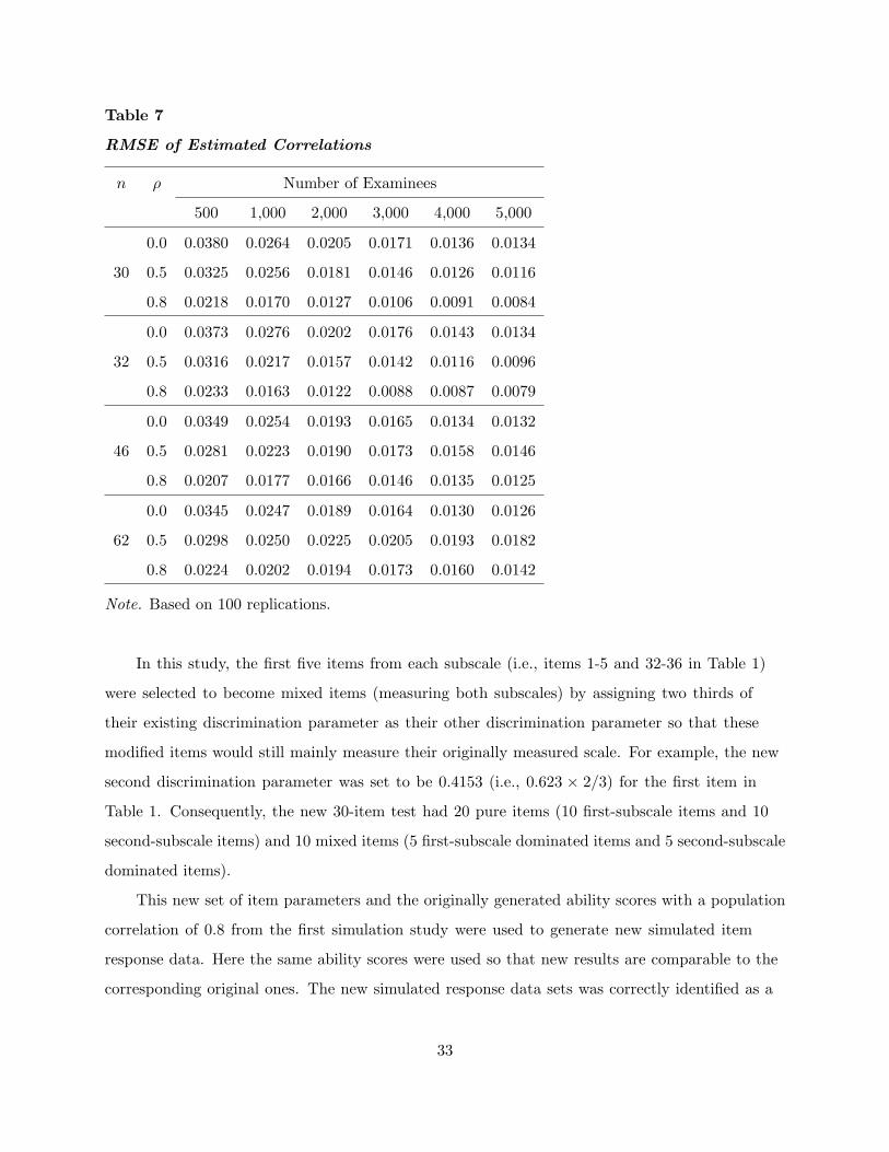
Table 7

RMSE of Estimated Correlations

n ρ Number of Examinees

500 1,000 2,000 3,000 4,000 5,000

0.0 0.0380 0.0264 0.0205 0.0171 0.0136 0.0134

30 0.5 0.0325 0.0256 0.0181 0.0146 0.0126 0.0116

0.8 0.0218 0.0170 0.0127 0.0106 0.0091 0.0084

0.0 0.0373 0.0276 0.0202 0.0176 0.0143 0.0134

32 0.5 0.0316 0.0217 0.0157 0.0142 0.0116 0.0096

0.8 0.0233 0.0163 0.0122 0.0088 0.0087 0.0079

0.0 0.0349 0.0254 0.0193 0.0165 0.0134 0.0132

46 0.5 0.0281 0.0223 0.0190 0.0173 0.0158 0.0146

0.8 0.0207 0.0177 0.0166 0.0146 0.0135 0.0125

0.0 0.0345 0.0247 0.0189 0.0164 0.0130 0.0126

62 0.5 0.0298 0.0250 0.0225 0.0205 0.0193 0.0182

0.8 0.0224 0.0202 0.0194 0.0173 0.0160 0.0142

Note. Based on 100 replications.

In this study, the first five items from each subscale (i.e., items 1-5 and 32-36 in Table 1)

were selected to become mixed items (measuring both subscales) by assigning two thirds of

their existing discrimination parameter as their other discrimination parameter so that these

modified items would still mainly measure their originally measured scale. For example, the new

second discrimination parameter was set to be 0.4153 (i.e., 0.623 × 2/3) for the first item in

Table 1. Consequently, the new 30-item test had 20 pure items (10 first-subscale items and 10

second-subscale items) and 10 mixed items (5 first-subscale dominated items and 5 second-subscale

dominated items).

This new set of item parameters and the originally generated ability scores with a population

correlation of 0.8 from the first simulation study were used to generate new simulated item

response data. Here the same ability scores were used so that new results are comparable to the

corresponding original ones. The new simulated response data sets was correctly identified as a

33

two-dimensional ASST using DETECT. Hence, when running ASSEST, each item was correctly

assigned to its dominant subscale in this study.

ASSEST was applied to the simulated response data with two different sets of specifications.

First, the simulated response data set was treated incorrectly as two-dimensional with simple

structure. Second, the data were correctly specified as two-dimensional with mixed simple

structure. In the former, both the unidimensional and multidimensional approaches can be applied

as before. The results from the unidimensional approach are not reported here since they are

similar to the corresponding results from the multidimensional approach. In the latter case, only

the multidimensional approach can be applied. The whole process was replicated 100 times and

the results are summarized in the last two columns of Table 8. The results in the second column

of Table 8 are from the first simulation study (see the eighth row in Table 5 and the fifth row in

Table 7) and serve as reference values here. Under the assumption that each item was correctly

assigned to its dominant subscale but the test itself was regarded as an SST, the ARMSE of

the estimated IRFs based on 100 replications was 0.0409 for 1,000 examinees, while the original

one (using the original SST data) was 0.0223. The new average estimated correlation between

subscales was 0.9059, while the original average of estimated correlations was 0.8043. Results are

similar in the cases of 3,000 and 5,000 examinees. Because the 10 mixed items were incorrectly

specified as pure items, ASSEST actually calibrated two composites, which were the combinations

of the target subscales, as discussed in Section 2.4. These two composite subscales leaned closer to

each other than the target subscales did. Not surprisingly, the correlation between target subscales

was overestimated. By (31), one may approximately calculate the expected correlation coefficient.

In the case here, α11 = 15.183, α12 = 3.139, α21 = 2.805, and α22 = 14.055. Hence, by (30), the

expected value of the correlation between the calibrated subscales is approximately 0.9070. When

the number of examinees is 5,000, the average estimated correlation is 0.9060, which is very close

to this expected value.

When the 10 modified items were correctly treated as mixed items (i.e., the data was treated

as an MSST instead of an SST), the ARMSE of the estimated IRF and the RMSE of the estimated

correlation are dramatically reduced (see the last column of Table 8). For instance, the ARMSE

of the estimated IRFs is 0.0180 for 3,000 examinees compared to 0.0350 when the modified items

were incorrectly treated as pure items. The average estimated correlation between subscales is

0.8057 in the case of 3,000 examinees while its counterpart is 0.9054 in the mistreated case. These

34

results indicate that it is inappropriate to treat an ASST as an SST.

Table 8

Summary Results for 30-item Test With 10 Mixed Items and 0.8 Correlation

Original SST ASST Calibrated ASST Calibrated

as an SST as an MSST

Number of Examinees = 1,000

ARMSE of Est. IRF 0.0223 0.0409 0.0263

(Its SD) (0.0023) (0.0020) (0.0029)

Average Est. Correlation 0.8043 0.9059 0.8071

(Its SD) (0.0186) (0.0104) (0.0224)

RMSE of Est. Correlation 0.0170 0.1065 0.0205


ARMSE of Est. IRF 0.0139 0.0350 0.0180

(Its SD) (0.0018) (0.0015) (0.0024)


(Its SD) (0.0115) (0.0063) (0.0125)



ARMSE of Est. IRF 0.0115 0.0335 0.0158

(Its SD) (0.0017) (0.0014) (0.0025)


(Its SD) (0.0093) (0.0051) (0.0102)


Note. Using the multidimensional approach, based on 100 replications.

4 Discussion

The simple structure assumption is widely used in the statistical analysis of data from many

testing programs. Until now, there are few testing programs that consider their tests to be more

complex than simple structure in operational data analysis. Many test frameworks or blueprints

35

require their tests to be of simple structure, that is, every item simply measures only one

subscale. This study shows that the simple structure assumption should be verified before doing

any statistical analysis based on it. As the second simulation study demonstrates, even a mild

violation may yield misleading results. In particular, the estimated correlation between subscales

will be overestimated if an ASST is mistreated as an SST. Hence, it is crucial to verify the simple

structure of a test even after its approximate simple structure has been identified. Although the

simple structure assumption is less stringent than the unidimensionality assumption of a whole

test, it is more complicated to check/test simple structure than just to check unidimensionality.

As discussed in Section 1, a two-step dimensionality analysis can be used to check the simple

structure of response data. The first step is to check if response data have approximate simple

structure. If so, the next step is to check the unidimensionality of each subtest.

After calibration, the estimated item parameters are usually treated as fixed in any further

analysis of response data. Therefore, the accuracy of estimated item parameters plays a very

important role in the analysis. Under the simple structure assumption, both the unidimensional

and multidimensional approaches can be used to estimate item parameters. This paper has proved

that these two approaches are theoretically the same if the joint maximum likelihood method is

used to estimate item parameters. However, when the marginal maximum likelihood method is

applied, the estimates of item parameters obtained from these two approaches are different. A

simulation study was conducted to further compare the unidimensional and multidimensional

approaches with the marginal maximum likelihood method. The simulation results reveal that

when the number of items is small the multidimensional approach provides relatively more

accurate estimates of item parameters; otherwise, the unidimensional approach prevails.

It should be noted that the unidimensional approach discussed in this paper has a different

focus than the unidimensional approximation approach that applies unidimensional models to

multidimensional item response data (see Reckase, Carlson, Ackerman, & Spray, 1986; Wang,

1988; Ackerman, 1989; Walker & Beretvas, 2003). The former applies unidimensional models

to each unidimensional subtest and the latter tries to approximate a test with unidimensional

models. When simple structure does not hold, the unidimensional approach deals with the same

problem as the unidimensional approximation approach does with each subtest. In this case,

however, the multidimensional approach should be used without simple structure constraints.

Future research may focus on the comparison of the accuracy of ability estimates between the

36

unidimensional and multidimensional approaches. Specifically, I may investigate how different

estimation approaches actually affect important measurement outcomes, such as pass/fail decision

consistency or placement decisions. Further research is also needed when a decision has to be

made whether to use the multidimensional approach or the unidimensional approach in the

analysis of complex matrix designed multiscale assessments, such as NAEP. The impact of such a

complex design has to be carefully investigated.

37

References

Ackerman, T. A. (1989). Unidimensional IRT calibration of compensatory and noncompensatory

multidimensional items. Applied Psychological Measurement, 13, 113-127.

Allen, N., Carlson, J. E., & Zelenak, C. (1999). The NAEP 1996 technical report (NCES

1999-452). Washington, DC: Office of Educational Research and Improvement, U.S.

Department of Education.

Allen, N., Donoghue, J. R., & Schoeps, T. L. (2001). The NAEP 1998 technical report (NCES

2001-509). Washington, DC: Office of Educational Research and Improvement, U.S.

Department of Education.

Allen, N., Kline, D., & Zelenak, C. (1997). The NAEP 1994 technical report (NCES 97-897).

Washington, DC: Office of Educational Research and Improvement, U.S. Department of

Education.

Bock, R. D., & Aitkin, M. (1981). Marginal maximum likelihood estimation of item parameters:

Application of the EM algorithm. Psychometrika, 46, 443-459.

Fraser, C., & McDonald, R. P. (1988). NOHARM: Least squares item factor analysis.

Multivariate Behavioral Research, 23, 267-269.

Hambleton, R. K., & Swaminathan, H. (1985). Item response theory: Principles and

applications. Boston: Kluwer-Nijhoff Publishing.

Lord, F. M. (1980). Applications of item response theory to practical testing problems. Hillsdale,

NJ: Lawrence Erlbaum Associates.

Michalewicsz, Z. (1994). Genetic algorithms + data structures = genetic programs. Berlin:

Springer-Verlag.

Mislevy, R. (1991). Randomization-based inference about latent variables from complex samples.

Psychometrika, 56, 177-196.

Mislevy, R., & Bock, R. D. (1982). BILOG: Item analysis and test scoring with binary logistic

models [Computer software]. Mooresville, IN: Scientific Software, Inc.

Muraki, E., & Bock, R. D. (1991). PARSCALE: Parameter scaling of rating data [Computer

software]. Chicago, IL: Scientific Software, Inc.

National Assessment Governing Board. (1994). Mathematics framework for the 1996 National

Assessment of Educational Progress. Washington, DC: National Assessment Governing

Board.

38

Reckase, M. D. (1985). The difficulty of test items that measure more than one ability. Applied

Psychological Measurement, 9, 401-412.

Reckase, M. D., Ackerman, T. A., & Carlson, J. E. (1988). Building a unidimensional test using

multidimensional items. Journal of Educational Measurement, 25, 193-203.

Reckase, M. D., Carlson, J. E., Ackerman, T. A., & Spray, J. A. (1986, June). The interpretation

of unidimensional IRT parameters when estimated from multidimensional data. Paper

presented at the annual meeting of the Psychometrika, Toronto, Canada.

Reckase, M. D., & McKinley, R. L. (1991). The discriminating power of items that measure

more than one dimension. Applied Psychological Measurement, 15, 361-373.

Stout, W. F. (1987). A nonparametric approach for assessing latent trait dimensionality.

Psychometrika, 52, 589-617.

Stout, W. F., Habing, B., Douglas, J., Kim, H. R., Roussos, L. A., & Zhang, J. (1996).

Conditional covariance based nonparametric multidimensionality assessment. Applied

Psychological Measurement, 20, 331-354.

Walker, C. M., & Beretvas, S. N. (2003). Comparing multidimensional and unidimensional

proficiency classifications: Multidimensional IRT as a diagnostic aid. Journal of Educational

Measurement, 40, 255-275.

Wang, M. (1987). Fitting a unidimensional model on the multidimensional item response data

(ONR Technical Report 87-1). University of Iowa.

Wang, M. (1988, April). Measurement bias in the application of a unidimensional model to

multidimensional item response data. Paper presented at the annual meeting of American

Educational Research Association, New Orleans, LA.

Zhang, J. (1996). Some fundamental issues in item response theory with applications.

Unpublished doctoral dissertation, Department of Statistics, University of Illinois at

Urbana-Champaign.

Zhang, J. (2000, April). Estimating multidimensional item response models with approximate

simple structure. Paper presented at the annual meeting of the National Council on

Measurement in Education, New Orleans, LA.

Zhang, J., & Lu, T. (2001, April). Evaluating the performance of ASSEST: A new item

parameter estimation program for multidimensional item response theory models. Paper

presented at the annual meeting of the National Council on Measurement in Education,

39

Seattle, WA.

Zhang, J., & Stout, W. F. (1999a). Conditional covariance structure of generalized

compensatory multidimensional items. Psychometrika, 64, 129-152.

Zhang, J., & Stout, W. F. (1999b). The theoretical DETECT index of dimensionality and its

application to approximate simple structure. Psychometrika, 64, 213-249.

40

Appendix

Some Notation

n The number of items in the test

nk The number of items in subtest k for k = 1, . . . , d, and∑d

k=1 nk = n

Γ The set of all item parameters in the test

Γk The set of all item parameters in subtest k for k = 1, . . . , d, and Γ = (Γ1,Γ2, . . . ,Γd)

N The number of examinees

xj Item response vector of the jth randomly sampled examinee for the test,

xj = (x1j , . . . , xnj) for j = 1, . . . , N

xkj Item response vector of subtest k for k = 1, . . . , d, and xj = (x1j ,x2j , . . . ,xdj)

where xkj = (xn1+···+nk−1+1 j , . . . , xn1+···+nk j) for k = 1, . . . , d, and n0 = 0

X The N × n response data matrix of the test, X = (x′1,x

′2, . . . ,x

′N )

′ ≡

x1

x2

...

xN

Xk The N × nk response data matrix of subtest k for k = 1, . . . , d,

Xk = (x′k1,x

′k2, . . . ,x

′kN )

′for k = 1, . . . , d, and X = (X1,X2, . . . ,Xd)

θj Ability vector of the jth sampled examinee and θj = (θ1j , θ2j , . . . , θdj),

where θkj is the kth subscale ability of examinee j for j = 1, . . . , N and k = 1, . . . , d.

Θ The N × d ability matrix of N randomly sampled examinees,

Θ = (θ′1,θ

′2, . . . ,θ

′N )

′

Θk Ability vector of the kth subscale abilities of N examinees for k = 1, . . . , d,

Θk = (θk1, θk2, . . . , θkN )′for k = 1, . . . , d, and Θ = (Θ1,Θ2, . . . ,Θd)

Σ The d× d correlation matrix of latent ability vector

41

I.N. 726810

Documents

Comparison of Unidimensional and Multidimensional ... · Research Report Comparison of Unidimensional and Multidimensional Approaches to IRT Parameter Estimation Jinming Zhang October