Comparative Assessment of Software Quality Classification Techniques: An Empirical Case Study

Empirical Software Engineering, 9, 229–257, 2004.

# 2004 Kluwer Academic Publishers. Manufactured in The Netherlands.

Comparative Assessment of Software Quality

Classification Techniques: An Empirical Case Study

TAGHI M. KHOSHGOFTAAR [email protected]

Empirical Software Engineering Laboratory, Department of Computer Science and Engineering, Florida

Atlantic University, Boca Raton, FL 33431 USA

NAEEM SELIYA

Empirical Software Engineering Laboratory, Department of Computer Science and Engineering, Florida

Atlantic University, Boca Raton, FL 33431 USA

Editor: Audris Mockus

Abstract. Software metrics-based quality classification models predict a software module as either fault-

prone ( fp) or not fault-prone (nfp). Timely application of such models can assist in directing quality

improvement efforts tomodules that are likely tobe fpduringoperations, thereby cost-effectively utilizing the

software quality testing and enhancement resources. Since several classification techniques are available, a

relative comparative study of some commonly used classification techniques can be useful to practitioners.

We present a comprehensive evaluation of the relative performances of seven classification techniques

and/or tools. These include logistic regression, case-based reasoning, classification and regression trees

(CART), tree-based classification with S-PLUS, and the Sprint-Sliq, C4.5, and Treedisc algorithms. The

use of expected cost of misclassification (ECM), is introduced as a singular unified measure to compare the

performances of different software quality classification models. A function of the costs of the Type I (a

nfp module misclassified as fp) and Type II (a fp module misclassified as nfp) misclassifications, ECM is

computed for different cost ratios. Evaluating software quality classification models in the presence of

varying cost ratios is important, because the usefulness of a model is dependent on the system-specific costs

of misclassifications. Moreover, models should be compared and preferred for cost ratios that fall within

the range of interest for the given system and project domain. Software metrics were collected from four

successive releases of a large legacy telecommunications system. A two-way ANOVA randomized-

complete block design modeling approach is used, in which the system release is treated as a block, while

the modeling method is treated as a factor. It is observed that predictive performances of the models is

significantly different across the system releases, implying that in the software engineering domain

prediction models are influenced by the characteristics of the data and the system being modeled. Multiple-

pairwise comparisons are performed to evaluate the relative performances of the seven models for the cost

ratios of interest to the case study. In addition, the performance of the seven classification techniques is

also compared with a classification based on lines of code. The comparative approach presented in this

paper can also be applied to other software systems.

Keywords: Software quality classification, decision trees, case-based reasoning, logistic regression,

expected cost of misclassification, analysis of variance.

1. Introduction

The use of software in high-assurance and mission-critical systems increases the needto develop and quantify measures of software quality. Subsequently, software

metrics are useful in the timely prediction of high-risk components during thesoftware development process (Basili et al., 1996; Briand et al., 2002; Ping et al.,2002). Such a prediction enables software managers to target quality improvementefforts to the needed areas. For example, prior to the system test, identifying thecomponents that are likely to be faulty during operations can improve theeffectiveness of testing efforts. Various software quality modeling techniques havebeen developed and used in real-life software quality predictions.Classification-based modeling for software quality estimation is a proven

technique in achieving better software quality control (Ebert, 1996; Ohlsson et al.,1996, 1998; Schneidewind, 1995). Some classification techniques used for softwarequality estimation include optimal set reduction (Briand et al., 1993), logisticregression (Khoshgoftaar and Allen, 1999; Schneidewind, 2001), decision trees(Khoshgoftaar et al., 2000; Suarez and Lutsko, 1999; Takahashi et al., 1997), neuralnetworks (Khoshgoftaar et al., 1997; Paul, 1992; Pizzi et al., 2002), and case-basedreasoning (Ross, 2001). Software metrics-based quality classification models classifysoftware modules into groups. A two-group classification model is the mostcommonly used, in which program modules are grouped into classes such as, fault-prone ( fp) and not fault-prone (nfp).1 Software analysts interested in predictingwhether a software component will be fp or nfp, can utilize classification models toobtain the needed prediction. When associating with such models, two types ofmisclassification errors are encountered: Type I error, that is, a nfp component ispredicted as fp, and Type II error, i.e., a fp component is misclassified as nfp.Practically speaking, Type II errors are more severe in terms of softwaredevelopment costs and the organization’s reputation. They may involve inspectionand correction to components after they have been deployed for operations.In our previous empirical studies related to software quality classification

modeling, we have investigated several classification techniques, includingclassification and regression trees (CART) (Khoshgoftaar et al., 2000), tree-basedclassification with S-PLUS (Khoshgoftaar et al., 2002), the Treedisc algorithm(Khoshgoftaar and Allen, 2001), the C4.5 algorithm (Ponnuswamy, 2001; Quinlan,1993), the Sprint-Sliq algorithm (Khoshgoftaar and Seliya, 2002), logisticregression (Khoshgoftaar and Allen, 1999), and case-based reasoning (Ross,2001). Classification models were calibrated using case studies of different large-scale software systems, including the one presented in this paper. The models arecalibrated to classify software modules as either fp or nfp, as defined by the systembeing modeled.Software quality classification models are usually compared based on how

accurately they can classify (predict) observations. It has been observed that whencomparing two-group software quality classification models, their Type I and TypeII misclassification error rates are used (Ebert, 1996; Schneidewind, 1995). As anattempt to utilize a singular comparative measure, some researchers have used theoverall misclassification error rate of models. Though the Type I, Type II, andoverall misclassification error rates have been commonly used as accuracy measures,they may not necessarily be the most appropriate and effective measures. We nowexplain in the following paragraphs, why this is so.

230 KHOSHGOFTAAR AND SELIYA

When performing empirical studies with different classification methods(Khoshgoftaar and Allen, 1999, 2001; Khoshgoftaar et al., 2000; Khoshgoftaarand Seliya, 2002; Ponnuswamy, 2001; Ross, 2001), our research group has observeddifficulty in comparing different models based solely on the misclassification errorrates. For example, consider classification models built by two competing methods(‘‘A’’ and ‘‘B’’) using a given data set for the software system under consideration.The difficulty of using only the models’ error rates for comparison occurs whenmethod ‘‘A’’ (as compared to method ‘‘B’’) has a lower Type I error rate and ahigher Type II error rate. Moreover, the difficulty in comparing competing methodsbased solely on their error rates increases when multiple methods are to becompared. In addition, the problem is compounded when multiple data sets (orsystem releases) are used for evaluating the relative performances of two or moreclassification methods. We can see that the use of two measures (Type I and Type IIerror rates) makes it difficult to compare the performances of competing methods.However, if method ‘‘A’’ always performs better (has lower Type I and Type II errorrates) than method ‘‘B’’ across all data sets, then we can undoubtedly infer thatmethod ‘‘A’’ is better.A quick solution to using the two error rates as performance measures would be to

use the overall misclassification error rate. However, such an approach assumes thatthe corrective costs of the two misclassifications are equal, i.e., cost ratio of one.Since from a software engineering point of view, it is obvious that Type II errors aremore costly than Type I errors, the use of the overall misclassification error rate asan accuracy measure may lead to misleading results. An improved solution would beto utilize an appropriate singular measure to compare different classification modelsin the context of the software quality estimation problem. Since the inspection (andcorrective) costs and efforts involved with the Type I and Type II errors are(practically speaking) different, a unified measure that incorporates the two types ofcosts is warranted.This paper introduces the use of the expected cost of misclassification (ECM)

(Johnson and Wichern, 1992), as a singular measure to compare the performances ofdifferent software quality classification models. Though it is not claimed that theECM values of competing models may not fluctuate across the system releases, wenote that the comparison difficulty is reduced because only one performancemeasure is used to compare the competing techniques. In a previous study, weinvestigated the use of ECM to evaluate overfitting tendencies of a decision tree-based model (Khoshgoftaar and Allen, 2001). Since ECM integrates the project- andsystem-specific costs of the Type I and Type II errors into a singular measure, itprovides a practical measure to compare the accuracies and performances ofsoftware quality classification models. To our knowledge, this is the first study toinvestigate the use of ECM as a practical performance measure for evaluatingusefulness of software quality classification models.Very few studies that compare different software quality classification modeling

methods, have been performed. Ebert (1996) presents a comparative study of fivesoftware quality classification methods, which include: Pareto classification, crispclassification trees, factor-based discriminant analysis, neural networks, and fuzzy

COMPARATIVE ASSESSMENT OF SOFTWARE QUALITY 231

classification. The study uses two small-scale case studies, consisting of 67 (10software metrics) and 451 (six software metrics) modules, respectively. Based onthese two case studies, it was suggested that among the five methods compared, fuzzyclassification is a better method. The different modeling methods were comparedusing the Type I and Type II misclassification error rates, the use of which (asdiscussed earlier) can lead to dubious results.This paper presents a comparative analysis of seven different classification

modeling methods for a case study of a large-scale legacy telecommunications (high-assurance) system. Software metrics and fault data were collected over foursuccessive system releases. The 28 software metrics that we used consist of softwareproduct and execution metrics. Other case studies of the legacy system were alsoperformed, however, they are not presented due to similarity of results andconclusions. When building classification models with the different techniques, acommon model building and validation approach was followed.The model-selection strategy adopted for the case study consisted of obtaining the

preferred balance (see Sections 4.1 and 4.3) of equality between the two error rates,with Type II being as low as possible. This implies that among the different (bychanging respective parameters) models obtained for a given classification technique,the model-selection strategy is such that priority is given to models that yield anapproximately equal balance between the two error rates, and among such models amodel that has the lowest Type II error is selected as the final model. Such anapproach was followed directly based upon our discussions with, and inputsprovided by, the project management team of the legacy system. The relativecomparison of the classification methods is based on their predictive performances(ECM values) in the context of varying cost ratios.Classification models built using CART (Khoshgoftaar et al., 2000), S-PLUS

(Khoshgoftaar et al., 2002), Treedisc algorithm (Khoshgoftaar and Allen, 2001),C4.5 algorithm (Ponnuswamy, 2001), Sprint-Sliq algorithm (Khoshgoftaar andSeliya, 2002), logistic regression (Khoshgoftaar and Allen, 1999), and case-basedreasoning (Ross, 2001) are compared in this paper. The first five are the tree-basedclassification techniques that were investigated by our research team. Since the costsof misclassifications may be influenced by the nature and required-reliability ofsoftware systems, we compare the seven methods at different cost ratios, CII=CI :ratio of costs of the Type II error rate ðCIIÞ and the Type I error rate ðCIÞ.Comparing classification models at different cost ratios will facilitate organiza-

tions to choose an appropriate modeling method, that performs best at a cost ratiowhich suits the software system being modeled. Based on our discussions with theproject management team of the legacy telecommunications system, a range of 20 to100 was identified as the likely cost ratio values for the high-assurance system.Therefore, our comparative evaluation is based on selected cost ratios that cover thepossible range for the legacy system. The ECM values of the classification models arecompared for cost ratios of 20, 25, 50, and 100.Performance comparison of different classification modeling methods is

performed by building two-way ANOVA randomized complete block design modelsfollowed by one-tailed multiple-pairwise comparisons of the seven modeling


techniques (Berenson et al., 1983). In the ANOVA models, we use system release(Releases 2, 3, and 4) as the ‘‘blocks’’ and the classification modeling methods as the‘‘factor’’. This is done to observe if the respective system releases and classificationmodels are significantly different from their respective counterparts. Release 1 wasnot used as a block since it was used to build or train the classification models. Thecomparative technique adopted in our study is not limited to only seven modelingmethods. It can be extended to compare fewer than, or more than, the number ofmethods compared in this paper. However, data from multiple releases or multipleprojects is needed to effectively utilize ANOVA design models for performancecomparisons of software quality classification models. In the case when softwaremetrics data is not available from multiple releases of a given system, similarperformance comparisons can be done by means of one-way ANOVA models.In addition to relatively comparing the seven classification techniques, we also

present a comparison of their classification performances with a software qualityclassification based on lines of code. This was done to investigate how the sevenclassification techniques perform with respect to classification based on a simplemethod.The layout of the rest of the paper is as follows. In Section 2, a brief description of

the different classification modeling methods is presented. In Section 3, the casestudy used in this paper is described. Section 4 discusses the modeling objective,methodology, and techniques employed in comparing the different classificationmodels. Sections 5 and 6 present the results and conclusions of our comparativestudy.

2. Software Quality Classification Techniques

This section presents a brief description of the classification methods compared inthis paper. The aim of this section is to give a brief overview of the classificationtechnique, and not (due to lack of space) to present an extensive algorithmic detail.Our research group has performed extensive empirical research in software qualityclassification modeling using all of the methods discussed. A generalized classifica-tion rule for model-building was adopted for all methods discussed.

2.1. CART

Classification and regression trees is a widely used decision tree system with manyapplications to data mining, predictive modeling, and data preprocessing (Breimanet al., 1984; Steinberg and Colla, 1995). CART is a statistical tool (Salford SystemsInc.) that automatically sifts large complex databases, searching for, discovering,and isolating significant patterns and relationships in the data. Our previous researchrelated to software quality classification include the use of CART (Khoshgoftaar etal., 2000).


The algorithms of CART search for questions that split nodes into relativelyhomogeneous child nodes, such as a group consisting largely of responders, or high-risk components. As the tree evolves, the nodes become increasingly morehomogeneous, identifying important segments. The set of predictor variables usedto split the nodes into segments, read directly off the tree and summarized in thevariable importance tables, are the key drivers of the response variable. Themethodology solves a number of performance, accuracy, and operational problemsthat still plague many current decision-tree methods. Some of innovations of CARTinclude: solving the tree size problem using strictly two-way splitting, incorporatingautomatic testing and validation, and providing a completely new method forhandling missing values in the data set.

2.2. S-PLUS

A solution for advanced data analysis, data mining, and statistical modeling (Clarkand Pregibon, 1992), the S-PLUS (Mathsoft Inc.) tool combines an intuitivegraphical user interface with an extensive data analysis environment to offer ease ofuse and flexibility. Among other data mining functions, S-PLUS includes regressiontree-based models.At the core of the S-PLUS system is S, a language designed specifically for data

visualization and exploration, statistical modeling and programming with data. Sprovides a rich, object-oriented environment designed for interactive data discovery.With a huge library of functions for all aspects of computing with data, S offers good

Table 1. Notations.

Symbol Description

ECM Expected cost of misclassification

NECM Normalized expected cost of misclassification

fp A fault-prone or high risk module

nfp A not fault-prone or low risk module

CI Cost of Type I misclassification error

CII Cost of Type II misclassification error

pfp Prior probability of fp modules

pnfp Prior probability of nfp modules

p The p-value for hypothesis testing

a The significance level for hypothesis testing

CBR Case-based reasoning (Leake, 1996; Ross, 2001)

LOG Logistic regression (Khoshgoftaar and Allen, 1999)

CART Classification and regression trees (Breiman et al., 1984)

SPT The Sprint-Sliq classification tree algorithm (Khoshgoftaar and Seliya, 2002;

Shafer et al., 1996)

TD The Treedisc classification tree algorithm (Khoshgoftaar and Allen, 2001)

S-PLUS The regression tree algorithm of S-PLUS (Khoshgaftaar et al., 2002)

C4.5 The C4.5 classification tree algorithm (Ponnuswamy, 2001; Quinlan, 1993)


extensibility. Our recent research related to software quality classification includedusing the regression tree algorithm of S-PLUS (Khoshgoftaar et al., 2002). In-depthmathematical details of the S-PLUS regression tree algorithm are presented in Clarkand Pregibon (1992). The predictors are software metrics treated by S-PLUS asordinal measures which are used to build regression trees to predict the responsevariable. Hereon, we use the notation S-PLUS to indicate the tool’s regression tree-based modeling algorithm.

2.3. C4.5 Algorithm

The C4.5 algorithm is an inductive supervised learning system which employsdecision trees to represent a quality model. C4.5 is a descendent of another inductionprogram, ID3 (Quinlan, 1993), and it consists of four principal programs: decisiontree generator, production rule generator, decision tree interpreter, and productionrule interpreter. The algorithm uses these four programs when constructing andevaluating classification tree models. Different tree models were built by varyingparameters: minimum node size before splitting and pruning percentage (Ponnus-wamy, 2001).The C4.5 algorithm commands certain pre-processing of data in order for it to

build decision tree models. Some of these include attribute value description type,predefined discrete classes, and sufficient number of observations for supervisedlearning. The classification tree is initially empty and the algorithm begins addingdecision and leaf nodes, starting with the root node.

2.4. Treedisc Algorithm

The Treedisc algorithm is a SAS macro implementation of the modified CHi-squareAutomatic Interaction Detection algorithm (Khoshgoftaar and Allen, 2001). Itconstructs a regression tree from an input data set, that predicts a specifiedcategorical response variable based on one or more predictors. The predictorvariable is selected to be the variable that is most significantly associated with thedependent variable according to a chi-squared test of independence in thecontingency table.Regression tree-based models are built by varying model parameters in order to

achieve the preferred balance between the misclassification error rates, and to avoidoverfitting of classification trees. A generalized classification rule is used to label eachleaf node after the regression tree is built. This classification rule is very similar to theapproach followed, when using S-PLUS regression trees as classification trees(Khoshgoftaar et al., 2002).


2.5. Sprint-Sliq algorithm

Sprint-Sliq is an abbreviated version of Scalable PaRallelizable INduction ofdecision Trees-Supervised Learning In Quest (Mehta et al., 1996; Shafer et al., 1996).The algorithm can be used to build classification tree models that can analyze bothnumeric and categorical attributes. It is a modified version of the classification treealgorithm of CART, and uses a different pruning technique based on the minimumdescription length principle (Mehta et al., 1995). The algorithm has excellentscalability and analysis speed. Classification tree modeling using Sprint-Sliq isaccomplished in two phases: a tree building phase and a tree pruning phase. Thebuilding phase recursively partitions the training data until each partition is either‘‘pure’’ or meets the stop-splitting rules set by the user.The IBM Intelligent Data Miner tool, which implements the Sprint-Sliq

algorithm, was used by our research group to build classification trees (Khoshgof-taar and Seliya, 2002). Sprint-Sliq uses the Gini Index to evaluate the goodness ofsplit of all the possible splits (Shafer et al., 1996). A class assignment rule is needed toclassify modules as fp and nfp.

2.6. Logistic Regression

Logistic regression is a statistical modeling technique that offers good modelinterpretation. Independent variables in logistic regression may be categorical,discrete or continuous. However, the categorical variables need to be encoded(e.g., 0, 1) to facilitate classification modeling. Our research group has used logisticregression to build software quality classification models (Khoshgoftaar and Allen,1999).Let xj be the jth independent variable, and let xi be the vector of the ith module’s

independent variable values. A module being fp is designated as an ‘‘event’’. Let q bethe probability of an event, and thus q=ð1� qÞ is the odds of an event. The logisticregression model has the form,

logq

1� q

� �¼ b0 þ b1x1 þ � � � þ bjxj þ bmxm ð1Þ

where, log means the natural logarithm, bj is the regression coefficient associatedwith independent variable xj, and m is the number of independent variables.Logistic regression suits software quality modeling because most software

engineering measures do have a monotonic relationship with faults that is inherentin the underlying processes. Given a list of candidate independent variables and asignificance level, a, some of the estimated coefficients may not be significantlydifferent from zero. Such variables should not be included in the final model.


2.7. Case-Based Reasoning

Case-based reasoning (CBR) (Kolodner, 1993; Leake, 1996), is a technique that aimsto find solutions to new problems based on past experiences, which are representedby ‘‘cases’’ in a ‘‘case library’’. The case library and the associated retrieval anddecision rules constitute a CBR model. In the context of a classification problem,each case in the case library has known attributes and class membership. Theworking hypothesis of CBR for software quality classification modeling is that amodule currently under development is probably fp if a module with similarattributes in an earlier release (or similar project) was fp.A CBR system can take advantage of availability of new or revised information by

adding new cases or by removing obsolete cases from the case library. Its goodscalability provides fast retrieval even as the size of the case library scales up. CBRsystems can be designed to alert users when a new case is outside the bounds ofcurrent experience. Our research group was the first to use CBR in the context ofbuilding and evaluating software metrics-based quality classification models (Ross,2001). A generalized classification rule, similar to the ones used in Khoshgoftaar andAllen (2000), is utilized to classify modules as fp or nfp.

3. Case Study Description

The case study data was collected over four successive releases, from a very largelegacy telecommunications system (LLTS). The software system is an embedded-computer application that included finite-state machines. Using the proceduraldevelopment paradigm the software was written in PROTEL (a high-level language)and was maintained by professional programrs in a large organization. A softwaremodule was considered as a set of related source-code files. Fault data was collectedat the module-level by the problem reporting system, and consisted of post-releasefaults discovered by customers during system operations. Faults were recorded onlyif their discovery resulted in changes to the source code of the respective module.Preventing discovery of faults after deployment was a high priority for thedevelopers, because visits to customer sites involved extensive consumption ofmonetary and other resources.Configuration management data analysis identified software modules that were

unchanged from the prior release. Fault data collected from the problem reportingsystem were tabulated into problem reports and anomalies were resolved. Due to thenature of the system being modeled, that is, a high-assurance system, the number ofmodules associated with post-release faults were very few as compared to moduleswith no faults. Two clusters of modules were identified: unchanged and updated. Theupdated modules consisted of those that were either new or had at least one updateto their source code since the prior release. Among the unchanged modules, almostall of them had no faults, and therefore, were not considered for modeling purposes.We selected updated modules with no missing data in relevant variables. These

updated modules had several millions lines of code, with a few thousand of these


modules in each system release. The number of updated modules (that remainedafter unchanged modules or those with missing data were removed) that wereconsidered for each of the four release are: 3649 for Release 1, 3981 for Release 2,3541 for Release 3, and 3978 for Release 4. A module was considered as nfp if it hadno post-release faults, and fp otherwise.The distribution of the post-release faults for each release is summarized in Table

2. The proportion of modules with no faults among the updated modules of Release1 was pnfp ¼ 0:937, and the proportion with at least one fault was pfp ¼ 0:063. Weobserve that the percentage of modules with no faults generally increases acrosssuccessive releases. This is to be expected for a legacy system in an environmentsimilar to that of LLTS, because the development process for such a high-assurancesoftware system generally tends to improve with time. However, this may not holdfor another software system because other factors such as new development staff orchanges in system functionality could increase the number of faults and introduceadditional fp modules.The set of available software metrics is usually determined by pragmatic

considerations. A data mining approach is preferred in exploiting software metricsdata (Fayyad, 1996), by which a broad set of metrics are analyzed rather thanlimiting data collection according to predetermined research questions. Datacollection for LLTS involved extracting source code from the configurationmanagement system. Measurements were recorded using the EMERALD softwaremetrics analysis tool (Khoshgoftaar et al., 2000). Preliminary data analysis selectedmetrics that were appropriate for our modeling purposes. Software metrics collectedincluded 24 product metrics, 14 process metrics and four execution metrics. The 14process metrics were not used in our empirical evaluation, because this studyexplores prediction of fp (and nfp) modules for software quality modeling after thecoding (implementation) phase and prior to system tests. The case study, consists of28 independent variables (Tables 3 and 4) that were used to predict the responsevariable: Class which identifies a software module either as fp or nfp.The software product metrics in Table 3 are based on call graph, control flow

graph, and statement metrics. An example of call graph metrics is number of distinctprocedure calls. A module’s control flow graph consists of nodes and arcs depicting

Table 2. Distribution of faults discovered by customers.

Percentage of updated modules

Faults Release 1 (%) Release 2 (%) Release 3 (%) Release 4 (%)

0 93.7 95.3 98.7 97.7

1 5.1 3.9 1.0 2.1

2 0.7 0.7 0.2 0.2

3 0.3 0.1 0.1 0.1

4 0.1 *

6 *

9 *

*One module.


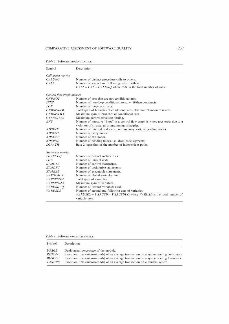
Table 3. Software product metrics.

Symbol Description

Call graph metrics

CALUNQ Number of distinct procedure calls to others.

CAL2 Number of second and following calls to others.

CAL2 ¼ CAL� CALUNQ where CAL is the total number of calls.

Control flow graph metrics

CNDNOT Number of arcs that are not conditional arcs.

IFTH Number of non-loop conditional arcs, i.e., if-then constructs.

LOP Number of loop constructs.

CNDSPNSM Total span of branches of conditional arcs. The unit of measure is arcs.

CNDSPNMX Maximum span of branches of conditional arcs.

CTRNSTMX Maximum control structure nesting.

KNT Number of knots. A ‘‘knot’’ in a control flow graph is where arcs cross due to a

violation of structured programming principles:

NDSINT Number of internal nodes (i.e., not an entry, exit, or pending node).

NDSENT Number of entry nodes.

NDSEXT Number of exit nodes.

NDSPND Number of pending nodes, i.e., dead code segments.

LGPATH Base 2 logarithm of the number of independent paths.

Statement metrics

FILINCUQ Number of distinct include files.

LOC Number of lines of code.

STMCTL Number of control statements.

STMDEC Number of declarative statements.

STMEXE Number of executable statements.

VARGLBUS Number of global variables used.

VARSPNSM Total span of variables.

VARSPNMX Maximum span of variables.

VARUSDUQ Number of distinct variables used.

VARUSD2 Number of second and following uses of variables.

VARUSD2 ¼ VARUSD� VARUSDUQ where VARUSD is the total number of

variable uses.

Table 4. Software execution metrics.

Symbol Description

USAGE Deployment percentage of the module.

RESCPU Execution time (microseconds) of an average transaction on a system serving consumers.

BUSCPU Execution time (microseconds) of an average transaction on a system serving businesses.

TANCPU Execution time (microseconds) of an average transaction on a tandem system.


the flow of control of the program. Statement metrics are measurements of theprogram statements without implying the meaning or logistics of the statements. Theproblem reporting system maintained records on past problems. The proportion ofinstallations that had a module, USAGE, was approximated by deployment data ona prior system release. Execution times in Table 4 were measured in a laboratorysetting with different simulated workloads.

4. Modeling Methodology

In this section, we present a brief discussion of the approach adopted in comparingthe different software quality classification modeling methods. We note that thedetails of classification modeling with the individual techniques have been omitted inthis paper due to paper-size concerns. Moreover, this has been done because thefocus of this study is to compare the various classification techniques we haveinvestigated in our previous studies. Please refer to the appropriate references for thedetails regarding the individual techniques (Khoshgoftaar and Allen, 1999, 2001;Khoshgoftaar et al., 2002, 2000; Khoshgoftaar and Seliya, 2002; Ponnuswamy, 2001;Ross, 2001).

4.1. Objective for Classification Models

In the case of high-assurance and mission-critical systems, due to the large disparitybetween the costs of misclassifications, it is highly desirable to detect and rectifyalmost all modules that are likely to be faulty during operations. As mentionedearlier, for a system similar to LLTS, the cost ratio is likely (based on practicalexperiences of similar projects) to fall within a range of 20 to 100. On the other hand,for a non-critical business application the cost ratio is likely to fall within the range10 to 25. The quality improvement needs of software projects are dependent on theapplication domain and the nature of the system being developed. Hence, whenevaluating techniques for calibrating classification models it is important that thepractical needs and objectives of the system being modeled are considered.While it is beneficial to detect prior to operations as many fp (actual) modules as

possible, the usefulness of a classification model is affected by the percentage ofactual nfp modules that are predicted as fp by the model, that is, a model’s Type Ierror rate. For example, despite capturing many of the actual fp modules, a modelwith a very low Type II error rate and a very high Type I error rate is not practicallyuseful. This is because, given the large number of modules predicted as fp (many ofthem are actually nfp), deploying the limited quality improvement resources will posea difficulty.Therefore, a more useful model is one that can obtain a preferred balance between

the error rates, according to the needs of the system being modeled. In the context oftwo-group classification modeling, an inverse relationship is observed between theType I and Type II error rates (Khoshgoftaar and Allen, 1999, 2001; Khoshgoftaar


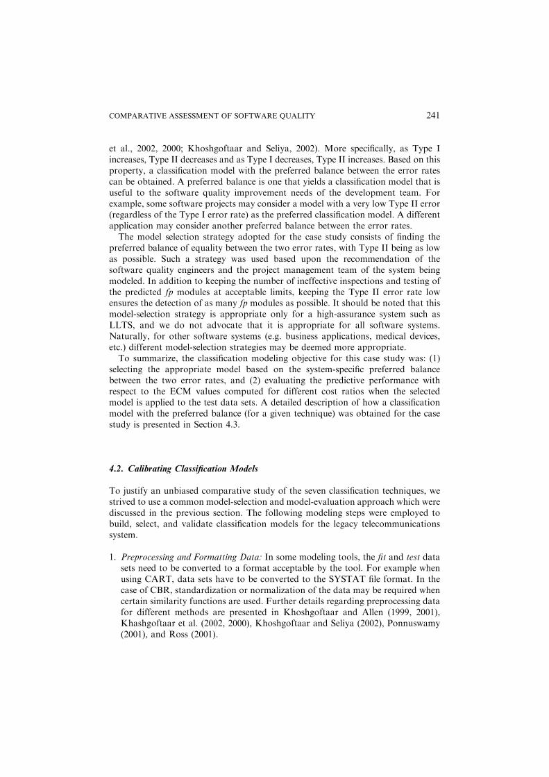
et al., 2002, 2000; Khoshgoftaar and Seliya, 2002). More specifically, as Type Iincreases, Type II decreases and as Type I decreases, Type II increases. Based on thisproperty, a classification model with the preferred balance between the error ratescan be obtained. A preferred balance is one that yields a classification model that isuseful to the software quality improvement needs of the development team. Forexample, some software projects may consider a model with a very low Type II error(regardless of the Type I error rate) as the preferred classification model. A differentapplication may consider another preferred balance between the error rates.The model selection strategy adopted for the case study consists of finding the

preferred balance of equality between the two error rates, with Type II being as lowas possible. Such a strategy was used based upon the recommendation of thesoftware quality engineers and the project management team of the system beingmodeled. In addition to keeping the number of ineffective inspections and testing ofthe predicted fp modules at acceptable limits, keeping the Type II error rate lowensures the detection of as many fp modules as possible. It should be noted that thismodel-selection strategy is appropriate only for a high-assurance system such asLLTS, and we do not advocate that it is appropriate for all software systems.Naturally, for other software systems (e.g. business applications, medical devices,etc.) different model-selection strategies may be deemed more appropriate.To summarize, the classification modeling objective for this case study was: (1)

selecting the appropriate model based on the system-specific preferred balancebetween the two error rates, and (2) evaluating the predictive performance withrespect to the ECM values computed for different cost ratios when the selectedmodel is applied to the test data sets. A detailed description of how a classificationmodel with the preferred balance (for a given technique) was obtained for the casestudy is presented in Section 4.3.

4.2. Calibrating Classification Models

To justify an unbiased comparative study of the seven classification techniques, westrived to use a common model-selection and model-evaluation approach which werediscussed in the previous section. The following modeling steps were employed tobuild, select, and validate classification models for the legacy telecommunicationssystem.

1. Preprocessing and Formatting Data: In some modeling tools, the fit and test datasets need to be converted to a format acceptable by the tool. For example whenusing CART, data sets have to be converted to the SYSTAT file format. In thecase of CBR, standardization or normalization of the data may be required whencertain similarity functions are used. Further details regarding preprocessing datafor different methods are presented in Khoshgoftaar and Allen (1999, 2001),Khashgoftaar et al. (2002, 2000), Khoshgoftaar and Seliya (2002), Ponnuswamy(2001), and Ross (2001).


2. Building Models: The modules of Release 1 were used as the fit data set to buildand select the respective classification models. Certain parameters specific to themodeling tool, are varied to build different classification models. For example,when using S-PLUS (Khoshgoftaar et al., 2002), mindev and minsize are varied tobuild different regression tree models. A generalized classification rule similar tothe one presented in Khoshgoftaar and Allen (2000) was used for all methods toclassify software modules as either fp or nfp.

3. Selecting Models: In order to validate our comparative study, it was importantthat model-selection for all the modeling techniques be based on the same dataset. For the case study, model-selection was based on the Release 2, i.e., based onthe misclassification error rates computed when Release 2 is used as the test dataset.

In the case of CART and CBR, model-selection was based on themisclassification error rates obtained from applying a cross-validation (Khosh-goftaar et al., 2000; Ross, 2001) technique on the fit (Release 1) data set. Cross-validation was not explicitly available for the other five modeling techniques.Since model-selection for two of the seven techniques was based on Release 1, wewere concerned with the model-selection validity of this comparative study. Upona close inspection of the Release 2 misclassification error rates for the differentCART and CBR models, we observed that the same model would have beenselected if Release 2 was used for model-selection purposes. Therefore, the model-selection validity of our comparative study is assured because the selected modelsfor the seven techniques remained unchanged when Release 2 is used for model-selection.

4. Evaluating Models: Releases 2, 3, and 4 are used as test data sets to evaluate the(predictive) classification accuracy of the different modeling techniques. Thecomputed Type I and Type II misclassification error rates (for the test datasets) are used to determine the ECM values for the different cost ratios thatwere considered. Only cost ratios that are likely for a system similar toLLTS were considered in our evaluation. The cost ratios considered are 20, 25,50, and 100.

4.3. Selecting a Preferred Model

In this section, we illustrate the description for obtaining the preferred balance withthe logistic regression classification technique (Khoshgoftaar and Allen, 1999).Similar descriptions for the other classification techniques can be obtained from therespective references. In the case of classification modeling with logistic regression, amodule being fp is designated as an ‘‘event’’.2 The maximum likelihood estimates ofthe model parameters ðbjÞ are computed using the iteratively re-weighted least


squares algorithm (Myers, 1990), where bj is the estimated value of bj (see Section2.6). The estimated logistic regression model takes the following form:

logeq̂q

1� q̂q

� �¼ b0 þ b1x1 þ � � � þ bjxj þ � � � þ bmxm ð2Þ

where q̂q is the estimate of the probability of a module being fp and 1� q̂q is theestimate of the probability of a module being nfp. The following procedure illustrateshow a logistic regression model can be used to classify program modules as either fpor nfp.

1. Compute q̂q=ð1� q̂qÞ using Equation (2).

2. Assign a module’s class, that is, ClassðxiÞ, by using the classification rule,

ClassðxiÞ ¼ nfp if 1�q̂qq̂q

� �> z

fp otherwise

(ð3Þ

where, z is a modeling parameter which can be empirically varied to obtain thepreferred classification model (Khoshgoftaar and Allen, 1999). In our case study,we varied the value of the parameter z to obtain the preferred balance between theerror rates.

The misclassification rates for the logistic regression models based on the differentvalues of z are presented in Table 5. The table only presents the error rates forReleases 1 and 2. The inverse relationship between the error rates is clearly observedwith respect to z. A very high value of z yielded a very low Type II error and a veryhigh Type I error. On the other hand, a very low value of z yielded a very high TypeII error and a very low Type I error. For example, when z ¼ 50 the correspondingfitted (Release 1) model yielded a Type I error rate of 67% and a Type II error rate of

Table 5. Preferred balance for logistic regression.

Release 1 Release 2

z Type I (%) Type II (%) Type I (%) Type II (%)

50 67.00 3.50 64.79 4.23

30 49.80 8.70 46.70 11.64

25 42.90 13.50 39.90 14.81

20 34.90 19.70 31.59 21.69

18 31.00 21.00 28.11 24.87

16 27.00 24.90 25.00 29.60

10 15.50 38.90 14.61 41.80

5 6.20 60.30 6.20 67.20

1 0.40 91.70 0.40 91.53

0.067 0.00 100.00 0.00 100.00


3.5%. Moreover, when z ¼ 1, the corresponding model yielded a Type I error rate of0.4% and a Type II error rate of 91.7%.According to the model-selection strategy described in Section 4.1, the preferred

balance (based on the fit data set, i.e., Release 1) was obtained when z ¼ 16. Weobserve that for z ¼ 16 the two error rates are approximately equal with the Type IIerror rate being low. Other values of z were also considered at the time of modeling,however, since they did not yield different empirical results, their correspondingmodels are not presented in the table.

4.4. Expected Cost of Misclassification

Recall, the cost of a Type I misclassification, CI , is the effort wasted on inspecting ortesting a nfp module. On the other hand, the cost of a Type II misclassification, CII ,is the rectification cost incurred due to the lost opportunity to correct faults prior tooperations. When the proportions of each class are approximately equal and thecosts of the misclassification for the system being modeled are approximately equal,the overall misclassification error rate can be a satisfactory measure of a model’spredictive accuracy. However, we have seen that in software applications of high-assurance and mission-critical systems, the proportion of fp modules is often verysmall in comparison to the proportion of nfp modules, and CII is usually severalmagnitudes greater than CI . Therefore, a model that yields a low ECM is preferred.The ECM measure (Equation (4)), takes prior probabilities of the two classes and

the costs of misclassifications into account (Johnson and Wichern, 1992). Since inmany organizations, it is not practical to quantify the individual costs ofmisclassifications, we normalize ECM3 with respect to CI (Equation (5)), facilitatingthe use of the cost ratio instead of individual misclassification costs.

ECM ¼ CIPrð fp j nfpÞpnfp þ CIIPrðnfp j fpÞpfp ð4Þ

NECM ¼ ECM

CI¼ Prð fp j nfpÞpnfp þ

CII

CIPrðnfp j fpÞpfp ð5Þ

The prior probabilities of the fp and nfp classes are given by, pfp and pnfprespectively. Prðfp j nfpÞ is the proportion of the nfp modules incorrectly classified asfp and conversely, Prðnfp j fpÞ is the proportion of the fp modules incorrectlyclassified as nfp. The prior probabilities, that is, pfp and pnfp, are estimated as therespective proportions in the given data set. We compared the classification modelsof the different modeling methods at different cost ratios, that is, by varying CII=CI

in Equation (5). Evaluating models across a range of cost ratios is more practicalsince the actual costs of misclassifications are unknown at the time of modeling.Moreover, the sensitivity (robustness) of a classification model in light of the possiblecosts and effort values, can be observed.It can be argued that advocating the use of ECM as a practical model-evaluation

measure can be extended for model-selection purposes. However, one has to becareful in doing so, because the selected model may not serve the practical quality


improvement objectives of the project management team, as discussed in Section 4.1.For example, for a cost ratio of 100 (empirical upper bound for high-assurancesystems) if a classification model demonstrates a very low Type II error rate and ahigh Type I error rate, then its ECM value is likely to be very low, leading toconclusion that it be selected as the preferred model.However, such a model is not useful for practical quality improvement purposes,

because a high Type I error rate indicates that many of the predicted fp modules areactually nfp. As discussed in Section 4.1, applying the limited resources allocated forsoftware quality improvement to all of the (a relatively large number) predicted fpmodules becomes infeasible. Inspecting a large number of modules according to thegiven organization’s software inspection and testing process may not be practicallypossible. Therefore, the first criterion for model-selection should be to respect theneeds of the software quality assurance team for the system being modeled. In ourstudy, model selection was done as per the recommendation provided by thesoftware quality engineers of the legacy system.We note that the use of ECM as a unified singular performance measure may

overlook some underlying predictive behavior of a classification model. Forexample, the prediction of a selected model may not yield a good preferred balancebut may yield a low ECM value. However, tracking the stability and robustness ofthe model performances (with respect to Type I and Type II errors) across the systemreleases is out of scope for this paper, and can be considered in future works.

4.5. Two-Way ANOVA: Randomized Complete Block Design

ANOVA, abbreviated for analysis of variance, is a commonly used statisticaltechnique when comparing differences between the means of three or moreindependent groups or populations. In our study, we employ the two-way ANOVA:Randomized complete block design modeling approach (Berenson et al., 1983; Neteret al., 1996), in which n heterogeneous subjects are classified into b homogeneousgroups, called blocks so that the subjects in each block can then be randomlyassigned, one each, to the levels of the factor of interest prior to the performance of atwo-tailed F test, to determine the existence of significant factor effects.Selecting the appropriate experimental design approach depends on the level of

reduction in experimental error required. Since the primary objective for selecting aparticular experimental design is to reduce experimental error (variability withindata), a better design could be obtained if subject variability is separated from theexperimental error (Neter et al., 1996). A two-way ANOVA randomized completeblock design is a restricted randomization design in which the experimental units arefirst sorted into homogeneous groups, i.e., blocks, and the treatments are thenassigned randomly within the blocks.We are interested in observing if the different modeling methods and the different

system releases are significantly different from their respective counterparts. Theobserved data for each release constitutes a replication. Since within each release, theobserved data is not affected by releases, blocking by release will reduce the


experimental error variability and will make the experiment more powerful(Berenson et al., 1983). We employ NECM predicted by different modeling methodsfor different releases as the response variable in our experimental design models.Since the analysis of variance models are based on some underlying assumptionssuch as normality of data and randomness of the variable, we note that anysignificant deviations from these assumptions were not observed.Experimental design models are built using NECM values computed for different

cost ratios. Two-way ANOVA models for our comparative study involved sevenfactor treatments (seven classification methods) and three blocks (system releases 2,3, and 4). The p-values (for different cost ratios) in the ANOVA design models(Table 7, later), indicate the significance of the difference between the variousmodeling methods as well as between the different system releases. To develop theANOVA procedure for a randomized complete block design, Yij , the observation inthe ith block of Bði ¼ 1; 2; . . . ; bÞ under the jth level of factor Að j ¼ 1; 2; . . . ; aÞ, canbe represented by the model,

Yi j ¼ mþ Aj þ Bi þ eij ð6Þ

where m ¼ overall effect or mean common to all observations; Aj ¼ m ? j � m, atreatment effect peculiar to the jth level of factor A (method); Bi ¼ m ? i � m, a blockeffect (system release) peculiar to the ith block of B; eij ¼ random variation orexperimental error associated with the observation in the ith block of B under the jthlevel of factor A; m ? j ¼ true mean for the jth level of factor A; m ? i ¼ true mean forthe ith block of B; Yij is an NECM value in the context of this paper.

4.6. Hypothesis Testing: A p-value Approach

Hypothesis testing is concerned with the testing of certain specified (i.e.,hypothesized) values for those population parameters. Statisticians and softwareanalysts alike, often perform hypothesis tests (Berenson et al., 1983) when comparingdifferent models. A null hypothesis, H0, is tested against its compliment, thealternate hypothesis, HA. Hypotheses are usually set up to determine if the datasupports a belief as specified by HA. These tests indicate the significance ðaÞ ofdifference between two methods or populations.The selection of the pre-determined significance level a, may depend on the analyst

and the project involved. In some cases the selection of a, may be too ambiguous ordifficult (Beaumont, 1996). In such situations, it may be preferred to performhypothesis testing without setting a value for a. This may be achieved by employingthe p-value approach to hypothesis testing (Beaumont, 1996; Berenson et al., 1983).This approach involves finding a value p, such that a given H0 will not be acceptedfor any a � p. Otherwise, H0 will not be rejected, that is, a < p. If this probability (p-value) is very high, H0 is not rejected, while if this likelihood is very small(traditionally lower than 0.05 or 0.1), H0 is rejected. Hypotheses tests may be


one-tailed or two-tailed, depending on the alternative hypothesis, HA, of interest tothe researcher (Beaumont, 1996; Berenson et al., 1983).We use the Minitab software tool (Beaumont, 1996), which has a provision for

statistical comparative analysis. We compute the p-values to determine if a method issignificantly better than another method. These p-values are used in deciding on theperformance order of the different tree-based classification methods. In makingdecisions regarding the rejection of H0, the appropriate test statistic would becompared against the critical values for the particular sampling distribution ofinterest. For our comparative study, we use the F statistic (Berenson et al., 1983). Ifthe F test statistic is distributed as Fðn1; n2Þ, then p-value is given by,

p ¼ PrfFð p; n1; n2Þ � Fðn1; n2Þg ð7Þ

where, n1 and n2 are the degrees of freedom for the F distribution, Fðp; n1; n2Þ is theentry in the F-table (Beaumont, 1996), and Fðn1; n2Þ is the computed statistic for thehypothesis test.

4.7. Multiple-Pairwise Comparison

The ANOVA block design models do not specify or indicate which means differfrom which of the other means. Multiple comparison methods facilitate a moredetailed information about the differences of these means. Specifically they provide astatistical technique to compare two methods (e.g. methods A and B) at a time. Avariety of multiple comparison methods are available, and for our study we employBonferroni’s multiple comparison equation (Beaumont, 1996; Berenson et al., 1983).Hypothesis testing using the p-value approach (see Section 4.6) is performed,yielding the p-value which indicates the level of difference between the two methodsbeing compared. The null and alternate hypotheses used for the multiple-pairwisecomparison study are given by,

H0 : NECMA � NECMB ð8ÞHA : NECMA < NECMB ð9Þ

4.8. Comparison with a Simple Method

A software quality assurance team of a given software project is often interested inknowing how well a given software quality model performs as compared toobtaining a model based on simple software metrics, such as software size. One ofthe most simple software metric is lines-of-code, which has often been used as a ruleof thumb to detect problematic software modules, i.e., the more the lines-of-code(LOC), the greater is the likelihood of having software faults. In addition toperforming a relative comparison of the seven classification techniques, we providethe classification results obtained by classifying modules as fp or nfp according totheir LOC.


The modules in the Release 1 (fit) data set are ordered in a descending order oftheir LOC, that is, the module at the top of the list has the most LOC and istherefore the most fp, while the module at the bottom of the list has the least LOCand is therefore the most nfp. Subsequently, starting from the top, the number ofmodules considered as fp according to LOC is varied until the two error rates satisfythe model selection strategy described in Section 4.1.Once the final model is selected according to classification based on LOC, the

number of modules considered as fp is recorded as is denoted by FPLOC.Subsequently, the modules in the test data sets, i.e., Releases 2, 3, and 4, areordered according to their LOC and the top FPLOC modules are considered as fp andthe Type I, Type II, and overall misclassification error rates are computed.Moreover, the respective expected cost of misclassification are also computed for thefour cost ratios mentioned earlier.

5. Results and Analysis

The results of our comparative analysis is based on observing the performances ofthe seven4 classification modeling techniques for the test data sets, that is, Releases 2,3, and 4. Release 1 was not included in the comparison, because it was used to trainthe individual models. Initially we wanted to consider evaluating the performancesof the seven techniques based solely on their Type I and Type II error rates.However, comparisons based on such an approach proved difficult and inappropri-ate, as discussed in Section 1.The predictive (on test data sets) performances of the seven models including the

Type I, Type II, and overall misclassification error rates and the NECM values forthe different cost ratios are presented in Table 6. These cost ratios represent the likelyrange for the legacy telecommunications system. For each of the techniques, thepreferred model was selected based on the practical model-selection strategy adoptedfor the legacy system. Our comparison goal is to observe (NECM values) the relativeperformances of the seven techniques, and if possible, suggest a relative rank-orderof their models. The comparative analysis and conclusions for each of the cost ratios,i.e., 20, 25, 50, and 100, is discussed at a significance level of 10%. This holds true forthe analysis of variance models and the multiple pairwise comparisons.The two-way ANOVA block design results for the seven techniques are presented

in Table 7. The NECM values computed for the test data sets, are used as theresponse variable for the ANOVA models. The notations used in Table 7 are asfollows: DF—degrees of freedom, SS—sums of squares, MS—mean squares, andF—the F statistic. The table indicates the respective p-values of whether the sevenmodels perform significantly different than each other, and whether the threereleases yield significantly different NECM values with respect to each other.We observe that for all the cost ratios, the NECM values across the three releases

(Releases 2, 3, and 4) are significantly different: p-values of less than or equal to0.1%. The difference in the performance across the system releases may be reflectiveof the software engineering domain. Shepperd and Kododa (2001) recently discussed


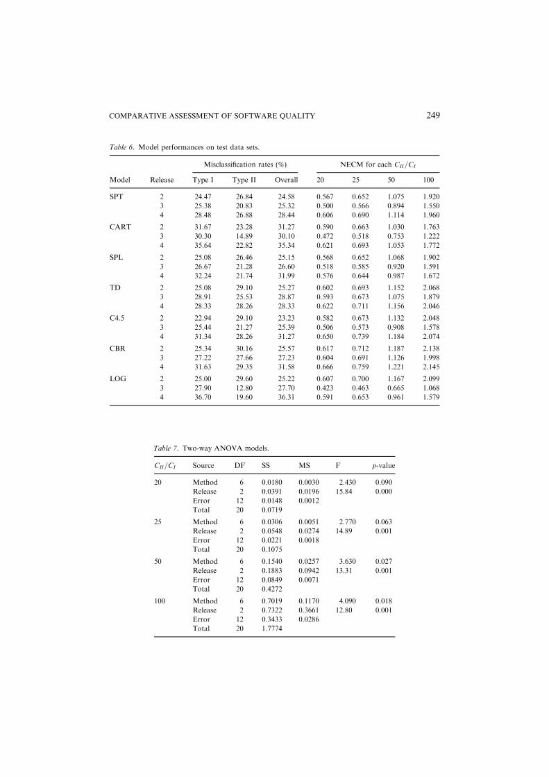
Table 7. Two-way ANOVA models.

CII=CI Source DF SS MS F p-value

20 Method 6 0.0180 0.0030 2.430 0.090

Release 2 0.0391 0.0196 15.84 0.000

Error 12 0.0148 0.0012

Total 20 0.0719

25 Method 6 0.0306 0.0051 2.770 0.063

Release 2 0.0548 0.0274 14.89 0.001

Error 12 0.0221 0.0018

Total 20 0.1075

50 Method 6 0.1540 0.0257 3.630 0.027

Release 2 0.1883 0.0942 13.31 0.001

Error 12 0.0849 0.0071

Total 20 0.4272

100 Method 6 0.7019 0.1170 4.090 0.018

Release 2 0.7322 0.3661 12.80 0.001

Error 12 0.3433 0.0286

Total 20 1.7774

Table 6. Model performances on test data sets.

Misclassification rates (%) NECM for each CII=CI

Model Release Type I Type II Overall 20 25 50 100

SPT 2 24.47 26.84 24.58 0.567 0.652 1.075 1.920

3 25.38 20.83 25.32 0.500 0.566 0.894 1.550

4 28.48 26.88 28.44 0.606 0.690 1.114 1.960

CART 2 31.67 23.28 31.27 0.590 0.663 1.030 1.763

3 30.30 14.89 30.10 0.472 0.518 0.753 1.222

4 35.64 22.82 35.34 0.621 0.693 1.053 1.772

SPL 2 25.08 26.46 25.15 0.568 0.652 1.068 1.902

3 26.67 21.28 26.60 0.518 0.585 0.920 1.591

4 32.24 21.74 31.99 0.576 0.644 0.987 1.672

TD 2 25.08 29.10 25.27 0.602 0.693 1.152 2.068

3 28.91 25.53 28.87 0.593 0.673 1.075 1.879

4 28.33 28.26 28.33 0.622 0.711 1.156 2.046

C4.5 2 22.94 29.10 23.23 0.582 0.673 1.132 2.048

3 25.44 21.27 25.39 0.506 0.573 0.908 1.578

4 31.34 28.26 31.27 0.650 0.739 1.184 2.074

CBR 2 25.34 30.16 25.57 0.617 0.712 1.187 2.138

3 27.22 27.66 27.23 0.604 0.691 1.126 1.998

4 31.63 29.35 31.58 0.666 0.759 1.221 2.145

LOG 2 25.00 29.60 25.22 0.607 0.700 1.167 2.099

3 27.90 12.80 27.70 0.423 0.463 0.665 1.068

4 36.70 19.60 36.31 0.591 0.653 0.961 1.579


the important relationship between the performance of a prediction technique andthe characteristics of the software metrics data. A recent work by Ohlsson andRuneson (2002) demonstrated that replicating empirical studies on classificationmodels in a context other than the original, can yield different results depending onhow different parameters are chosen. In the case of the legacy system studied in thispaper, it was observed that the software development process improved with time,i.e., the number of fp modules reduced over the different system releases.It is also seen in Table 7 that for all the cost ratios, the seven classification models

are different from each other at a 10% significance level. This was an important stepin our comparative study, because if the ANOVA models had revealed insignificantp-values for the ‘‘method’’ factor, then there would be no need to perform multiplepairwise comparisons to evaluate the relative differences of the seven models.However, since the p-values are significant, we proceeded with the pairwisecomparisons for all the seven methods. A given model among the seven is comparedwith the other six models using a one-tailed pairwise comparison. For example,CART is compared with SPL, SPT, TD, C4.5, LOG, and CBR individually. Thus,for each pair of methods (say A and B), we have two comparisons: is A better thanB? and is B better than A? The null and alternate hypotheses for the multiplepairwise comparisons are presented in Section 4.7.The p-values obtained from the multiple pairwise comparisons are presented in

Table 8. For a given cost ratio, the table can be viewed as a 767 matrix, i.e., eachpair of two methods forms a comparison. This implies that methods in the secondcolumn are compared with the methods listed in the headings of the tables. Examplecomparisons would be, fSPT vs. CART, CART vs. SPTg, fSPT vs. SPL, SPL vs.SPTg, and so on. A * in the table indicates the fact that a given model is notcompared to itself. Since we have seven modeling methods, there are 42 comparisonsfor each cost ratio. The p-values indicate the significance level of difference in theNECM values between two methods for a particular cost ratio.We are interested in determining (if possible) the performance order of these seven

models. To do so, we present our discussion based on the comparisons for one of thecost ratios shown in Table 8. Subsequently, similar analysis and discussions can bemade for the other cost ratios. Let us consider the comparisons for CII=CI ¼ 25. Aquick look at the p-values for this case indicates that many of the pairwisecomparisons are not statistically significant at a 10% significance level: shown by themany 1s. However, p-values of some of the comparisons are significant at 10%. Inthe next few paragraphs we analyze the p-values for this cost ratio, and comment onthe significance of their relative performances.When LOG is compared to CART, SPL, and SPT we observe that there are no

statistical differences (p-values of 1.000) in their relative performances, that is, allfour models essentially yielded similar NECM values for a cost ratio of 25. We alsoobserve that when compared to C4.5, the LOG model is not better ð p ¼ 0:399Þ atthe 10% significance level. However, when compared to CBR ð p ¼ 0:019Þ and TDð p ¼ 0:086Þ, its performance is significantly better. Observing the pairwisecomparisons between TD, C4.5, and CBR it is indicated that neither is significantlybetter than the other two.


If we denote LOG, CART, SPL, and SPT into one group (say A), and C4.5, TD,and CBR into another group (say B), we note that each of the models in a givengroup perform similar to the other models in that group. So practically speaking, ifone were to pick a model from each of the groups, then any of the respective modelscan be selected without significantly sacrificing performance. It is indicated that allthe models of group A are significantly better (at 10%) than the CBR model of groupB, as indicated by the respective p-values. All the models of group A, except LOG,do not perform better (or are similar) than the C4.5 and TD models of group B at the10% significance level. We observe an overlap between the two groups, i.e., theCART, SPL, and SPT models of group A and the C4.5, and TD models of group Bperformed similar. Therefore, among these five techniques any one can be pickedwithout significantly sacrificing performance.Therefore, for the cost ratio of 25 we can identify two performance-based clusters,

i.e., fLOG, CART, SPL, SPTg and fC4.5, TD, CBRg. The grouping of models intotwo clusters does not indicate that all models of group A are better than all models ofgroup B. It simply indicates that all models within their respective groups showed

Table 8. Multiple pairwise comparison: p-values.

CII=CI Model SPT CART SPL TD C4.5 CBR LOG

20 SPT * 1.000 1.000 0.371 1.000 0.086 1.000

CART 1.000 * 1.000 0.448 1.000 0.106 1.000

SPL 1.000 1.000 * 0.301 1.000 0.068 1.000

TD 1.000 1.000 1.000 * 1.000 1.000 1.000

C4.5 1.000 1.000 1.000 1.000 * 0.324 1.000

CBR 1.000 1.000 1.000 1.000 1.000 * 1.000

LOG 1.000 1.000 1.000 0.128 0.598 0.028 *

25 SPT * 1.000 1.000 0.402 1.000 0.098 1.000

CART 1.000 * 1.000 0.237 0.944 0.055 1.000

SPL 1.000 1.000 * 0.262 1.000 0.061 1.000

TD 1.000 1.000 1.000 * 1.000 1.000 1.000

C4.5 1.000 1.000 1.000 1.000 * 0.357 1.000

CBR 1.000 1.000 1.000 1.000 1.000 * 1.000

LOG 1.000 1.000 1.000 0.086 0.399 0.019 *

50 SPT * 1.000 1.000 0.513 1.000 0.145 1.000

CART 0.764 * 1.000 0.063 0.252 0.016 1.000

SPL 1.000 1.000 * 0.215 0.754 0.056 1.000

TD 1.000 1.000 1.000 * 1.000 1.000 1.000

C4.5 1.000 1.000 1.000 1.000 * 0.471 1.000

CBR 1.000 1.000 1.000 1.000 1.000 * 1.000

LOG 0.555 1.000 1.000 0.043 0.175 0.011 *

100 SPT * 1.000 1.000 0.598 1.000 0.188 1.000

CART 0.387 * 1.000 0.034 0.126 0.010 1.000

SPL 1.000 1.000 * 0.205 0.6592 0.059 1.000

TD 1.000 1.000 1.000 * 1.000 1.000 1.000

C4.5 1.000 1.000 1.000 1.000 * 0.561 1.000

CBR 1.000 1.000 1.000 1.000 1.000 * 1.000

LOG 0.372 1.000 0.997 0.033 0.119 0.009 *


similar performances with respect to their ECM values. As per the discussion in theprevious two paragraphs, there is clearly an overlap between the two clusters. A pureor strict ranking (at 10% significance) of all the seven models is not feasible for thiscase.The classification results obtained by ordering the modules of Release 1 and

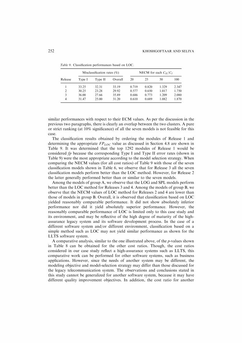
determining the appropriate FPLOC value as discussed in Section 4.8 are shown inTable 9. It was determined that the top 1292 modules of Release 1 would beconsidered fp because the corresponding Type I and Type II error rates (shown inTable 9) were the most appropriate according to the model selection strategy. Whencomparing the NECM values (for all cost ratios) of Table 9 with those of the sevenclassification models shown in Table 6, we observe that for Release 3 all the sevenclassification models perform better than the LOC method. However, for Release 2the latter generally performed better than or similar to the seven models.Among the models of group A, we observe that the LOG and SPL models perform

better than the LOC method for Releases 3 and 4. Among the models of group B, weobserve that the NECM values of LOC method for Releases 2 and 4 are lower thanthose of models in group B. Overall, it is observed that classification based on LOCyielded reasonably comparable performance. It did not show absolutely inferiorperformance nor did it yield absolutely superior performance. However, thereasonably comparable performance of LOC is limited only to this case study andits environment, and may be reflective of the high degree of maturity of the high-assurance legacy system and its software development process. In the case of adifferent software system and/or different environment, classification based on asimple method such as LOC may not yield similar performance as shown for theLLTS software system.A comparative analysis, similar to the one illustrated above, of the p-values shown

in Table 8 can be obtained for the other cost ratios. Though, the cost ratiosconsidered in our case study reflect a high-assurance systems such as LLTS, thiscomparative work can be performed for other software systems, such as businessapplications. However, since the needs of another system may be different, themodeling objective and model-selection strategy may differ than those discussed forthe legacy telecommunication system. The observations and conclusions stated inthis study cannot be generalized for another software system, because it may havedifferent quality improvement objectives. In addition, the cost ratio for another

Table 9. Classification performances based on LOC.

Misclassification rates (%) NECM for each CII=CI

Release Type I Type II Overall 20 25 50 100

1 33.25 32.31 33.19 0.719 0.820 1.329 2.347

2 30.25 23.28 29.92 0.577 0.650 1.017 1.750

3 36.00 27.66 35.89 0.686 0.773 1.209 2.080

4 31.47 25.00 31.20 0.610 0.689 1.082 1.870


software system may also be different. However, the comparative methodology cancertainly be applied to other systems for selecting a preferred model amongrespective competitors.In an empirical software engineering effort, threats to internal validity are

unaccounted influences that may affect case study results. In the context of thisstudy, poor estimates can be caused by a wide variety of factors, includingmeasurement errors while collecting and recording software metrics; modeling errorsdue to the unskilled use of software applications; errors in model-selection during themodeling process; and the presence of outliers and noise in the training data set.Measurement errors are inherent to the data collection effort, which has beendiscussed earlier. In our comparative study, a common model-building and model-selection approach have been adopted. Moreover, the statistical analysis (ANOVAmodels, pairwise comparison, etc.) was performed by only one skilled person inorder to keep modeling errors to a minimum.Threats to external validity are conditions that limit generalization of case study

results. To be credible, the software engineering community demands that the subjectof an empirical study be a system with the following characteristics (Votta andPorter, 1995): (1) developed by a group, rather than an individual; (2) developed byprofessionals, rather than students; (3) developed in an industrial environment,rather than an artificial setting; and (4) large enough to be comparable to realindustry projects. The software system investigated in this study meets all theserequirements.

6. Summary

Software quality estimation models can effectively minimize software failures,improving the operational-reliability of software-based systems. Many softwareapplications involve the use of software in high-assurance systems, which creates theneed to develop and quantify effective software quality prediction models. Thetimely prediction of fp components during the software development process canenable the software quality assurance team to target inspection and testing efforts tothose components. Software quality classification modeling techniques facilitate sucha timely estimation. Software metrics-based quality classification models, classifysoftware modules into classes.In this study, we compared the predictive performances of seven classification

methods which were used to build two-group classification models that classifiedmodules as either fp or nfp. The modeling methods that were compared includedCART, S-PLUS, the Sprint-Sliq algorithm, the C4.5 algorithm, the Treediscalgorithm, case-based reasoning, and logistic regression. The comparative study ispresented through a case study of a legacy telecommunications system. ANOVAblock design models are designed to study whether the classification methods weresignificantly different than each other with respect to their ECM values. The blockdesign was also used to investigate whether the system releases were significantlydifferent than each other with respect to a given model’s predictive performance.


Expected cost of misclassification is introduced as a unified singular performancemeasure for comparing different software quality classification models. The use ofECM was warranted because of the misleading tendencies and ambiguitiesassociated when Type I and Type II errors are used to compare differentclassification models. It incorporates the importance of misclassification costs onthe usefulness of classification models. The relative performances of the seven modelswas investigated by performing one-tailed multiple pairwise comparisons withrespect to their ECM values. Models were evaluated for a set of cost ratio values thatwere considered appropriate for the legacy telecommunications system, that is, 20 to100.We note that our comparative evaluation for the case study is based on comparing

only the ECM values of the different techniques. Other criteria, such as simplicity inmodel-calibration, complexity of model-interpretation, and stability of modelsacross releases may decide which modeling techniques are better than others. Wealso reiterate that the results of this paper cannot be generalized because thecomparative study is based on a single software system. Moreover, due to the lack ofintuition as to why some classification techniques sometimes behaved differentlythan others, it is not possible to draw a definitive conclusion about which method(s)will perform the best. We also note that the success/failure of a particular predictionmethod has a strong relationship with the characteristics of the estimation problem,specifically the characteristics of the data set(s) and the system domain (Shepperdand Kadoda, 2001).Future work may include, investigating a similar comparative study as the one

presented in this study, with software metrics and fault data from a software systemother than a telecommunications system.

Acknowledgments

We thank the three anonymous reviewers for their insightful comments. We alsothank the coordinating editor for providing useful suggestions. We thank John P.Hudepohl, Wendell D. Jones and the EMERALD team for collecting the necessarycase-study data. We also thank Meihui Mao for her assistance with data analysis andstatistical modeling. This work was supported in part by Cooperative AgreementNCC 2-1141 from NASA Ames Research Center, Software Technology Division,and Center Software Initiative for the NASA software IV&V Facility at Fairmont,West Virginia.

Notes

1. Some of the notations used in this paper are presented in Table 1.

2. This section only presents a discussion on how to obtain the preferred balance with logistic regression,

and is not meant to provide a complete classification procedure of the technique.


3. In the paper, the notation ECM refers to the normalized expected cost of misclassification (NECM),

and the two are used interchangeably.

4. The notations used for the different methods/techniques/tools are shown in Table 1.

References

Basili, V. R., Briand, L. C., and Melo, W. L. 1996. A validation of object-oriented design metrics as

quality indicators. IEEE Transactions on Software Engineering 22(10): 751–761, October.

Beaumont, G. P. 1996. Statistical Tests: An Introduction with Minitab Commentary. Prentice Hall.

Berenson, M. L., Levine, D. M., and Goldstein, M. 1983. Intermediate Statistical Methods and

Applications: A Computer Package Approach. Englewood Cliffs, NJ: Prentice Hall, USA.

Breiman, L., Friedman, J. H., Olshen, R. A., and Stone, C. J. 1984. Classification And Regression Trees.

Belmont, California, USA: Wadsworth International Group, 2nd edition.

Briand, L. C., Basili, V. R., and Hetmanski, C. J. 1993. Developing interpretable models with optimized

set reduction for identifying high-risk software components. IEEE Transactions on Software Engineering

19(11): 1028–1044, November.

Briand, L. C., Melo, W. L., and Wust, J. 2002. Assessing the applicability of fault-proneness models across

object-oriented software projects. IEEE Transactions on Software Engineering 28(7): 706–720.

Clark, L. A., and Pregibon, D. 1992. Tree-based models. In J. M. Chambers and T. J. Hastie, (eds),

Statistical Models in S. Wadsworth International Group, Pacific Grove, California,

pp. 377–419.

Ebert, C. 1996. Classification techniques for metric-based software development. Software Quality Journal

5(4): 255–272.

Fayyad, U. M. 1996. Data mining and knowledge discovery: Making sense out of data. IEEE Expert

11(4): 20–25.

Johnson, R. A., and Wichern, D. W. 1992. Applied Multivariate Statistical Analysis. Englewood Cliffs, NJ:

Prentice Hall, USA, 2nd edition.

Khoshgoftaar, T. M., and Allen, E. B. 1999. Logistic regression modeling of software quality.

International Journal of Reliability, Quality and Safety Engineering 6(4): 303–317.

Khoshgoftaar, T. M., and Allen, E. B. 2000. A practical classification rule for software quality models.

IEEE Transactions on Reliability 49(2): 209–216.

Khoshgoftaar, T. M., and Allen, E. B. 2001. Controlling overfitting in classification-tree models of

software quality. Empirical Software Engineering 6(1): 59–79.

Khoshgoftaar, T. M., Allen, E. B., and Deng, J. 2002. Using regression trees to classify fault-prone

software modules. IEEE Transactions on Reliability 51(4): 455–462.

Khoshgoftaar, T. M., Allen, E. B., Hudepohl, J. P., and Aud, S. J. 1997. Applications of neural networks

to software quality modeling of a very large telecommunications system. IEEE Transactions on Neural

Networks 8(4): 902–909.

Khoshgoftaar, T. M., Allen, E. B., Jones, W. D., and Hudepohl, J. P. 2000. Classification tree models of

software-quality over multiple releases. IEEE Transactions on Reliability 49(1): 4–11.

Khoshgoftaar, T. M., and Seliya, N. 2002. Software quality classification modeling using the SPRINT

decision tree algorithm. In Proceedings: 14th International Conference on Tools with Artificial

Intelligence. Washington, DC, USA: IEEE Computer Society, November, pp. 365–374.

Kolodner, J. 1993. Case-Based Reasoning. San Mateo, California USA: Morgan Kaufmann Publishers,

Inc.

Leake, D. B. (ed.) 1996. Case-Based Reasoning: Experience, Lessons, and Future Directions. Cambridge,

MA USA: MIT Press.

Mehta, M., Agarwal, R., and Rissanen, J. 1996. SLIQ: A fast scalable classifier for data mining. IBM

White Paper Series: Available at www.almaden.ibm.com/cs/quest, March.

Mehta, M., Rissanen, J., and Agarwal, R. 1995. MDL-based decision tree pruning. IBM White Paper

Series: Available at www.almaden.ibm.com/cs/quest, August.

Myers, R. H. 1990. Classical and Modern Regression with Applications. PWS-KENT, Boston, MA, USA.


Neter, J., Kutner, M. H., Nachtsheim, C. J., and Wasserman, W. 1996. Applied Linear Statistical Models.

4th edition. Chicago, IL, USA: Irwin McGraw-Hill.

Ohlsson, M. C., Helander, M., and Wohlin, C. 1996. Quality improvement by identification of fault-prone

modules using software design metrics. In Proceedings: International Conference on Software Quality,

Ottawa, Ontario, Canada, pp. 1–13.

Ohlsson, M. C., and Runeson, P. 2002. Experience from replicating empirical studies on prediction

models. In Proceedings: 8th International Software Metrics Symposium. Ottawa, Ontario, Canada: IEEE

Computer Society, June, pp. 217–226.

Ohlsson, N., Zhao, M., and Helander, M. 1998. Application of multivariate analysis for software fault

prediction. Software Quality Journal 7(1): 51–66.

Paul, R. 1992. Metric-based neural network classification tool for analyzing large-scale software. In

Proceedings: International Conference on Tools with Artificial Intelligence. Arlington, Virginia, USA:

IEEE Computer Society, November, pp. 108–113.

Ping, Y., Systa, T., and Muller, H. 2002. Predicting fault-proneness using OO metrics, an industrial case

study. In T. Gyimothy and F. B. Abreu (eds), Proceedings: 6th European Conference on Software

Maintenance and Reengineering. Budapest, Hungary, March, pp. 99–107.

Pizzi, N. J., Summers, A. R., and Pedrycz, W. 2002. Software quality prediction using median-adjusted

class labels. In Proceedings: International Joint Conference on Neural Networks, volume 3. Honolulu,

Hawaii, USA: IEEE Computer Society, May, pp. 2405–2409.

Ponnuswamy, V. 2001. Classification of software quality with tree modeling using C4.5 algorithm.

Master’s thesis, Florida Atlantic University, Boca Raton, Florida USA, December. Advised by Taghi

M. Khoshgoftaar.

Quinlan, J. R. 1993. Machine Learning, C4.5: Programs For Machine Learning. San Mateo, California:

Morgan Kaufmann.

Ross, F. D. 2001. An empirical study of analogy based software quality classification models. Master’s

thesis, Florida Atlantic University, Boca Raton, FL USA, August. Advised by T. M. Khoshgoftaar.

Schneidewind, N. F. 1995. Software metrics validation: Space shuttle flight software example. Annals of

Software Engineering 1: 287–309.

Schneidewind, N. F. 2001. Investigation of logistic regression as a discriminant of software quality. In

Proceedings: 7th International Software Metrics Symposium. London UK: IEEE Computer Society,

April, pp. 328–337.

Shafer, J., Agarwal, R., and Mehta, M. 1996. SPRINT: A scalable parallel classifier for data mining. IBM

White Paper Series: Available at www.almaden.ibm.com/cs/quest, September.

Shepperd, M., and Kadoda, G. 2001. Comparing software prediction techniques using simulation. IEEE

Transactions on Software Engineering 27(11): 1014–1022.

Steinberg, D., and Colla, P. 1995. CART: A supplementary module for SYSTAT. Salford Systems, San

Diego, California.

Suarez, A., and Lutsko, J. F. 1999. Globally optimal fuzzy decision trees for classification and regression.

Pattern Analysis and Machine Intelligence 21(12): 1297–1311, IEEE Computer Society.

Takahashi, R., Muraoka, Y., and Nakamura, Y. 1997. Building software quality classification trees:

Approach, experimentation, evaluation. In Proceedings: 8th International Symposium on Software

Reliability Engineering. Albuquerque, NM, USA: IEEE Computer Society: November, pp. 222–233.

Votta, L. G., and Porter, A. A. 1995. Experimental software engineering: A report on the state of the art.

In Proceedings of the 17th. International Conference on Software Engineering. Seattle, WA USA: IEEE

Computer Society, April, pp. 277–279.


Taghi M. Khoshgoftaar is a professor of the Department of Computer Science and Engineering, Florida

Atlantic University and the Director of the Empirical Software Engineering Laboratory. His research

interests are in software engineering, software complexity metrics and measurements, software reliability

and quality engineering, computational intelligence, computer performance evaluation, multimedia

systems, and statistical modeling. He has published more than 150 refereed papers in these areas. He has

been a principal investigator and project leader in a number of projects with industry, government, and

other research-sponsoring agencies. He is a member of the Association for Computing Machinery, the

IEEE Computer Society, and IEEE Reliability Society. He served as the general chair of the 1999 IEEE

International Symposium on Software Reliability Engineering (ISSRE’99). He was the recipient of the

Researcher of the Year Award at Florida Atlantic University for the year 2000. He is the general chair of

the 2001 IEEE International Symposium on High-Assurane Systems Engineering HASE’01). He has

served on technical program committees of various international conferences, symposia, and workshops.

He has served as North American editor of the Software Quality Journal, and was on the editorial board of

the Journal of Multimedia Tools and Applications.

Naeem Seliya recieved the MS degree in Computer Science from Florida Atlantic University, Boca Raton,

FL, USA, in 2001. He is currently a Ph.D. candidate in the Department of Computer Science and

Engineering at Florida Atlantic University. His research interests include software engineering with

computational intelligence, software metrics, software architecture, data mining, software quality and

reliability, object oriented design, and computer data security. He is student member of the IEEE

Computer Society and the Association for Computing Machinery.


Documents

Comparative Assessment of Software Quality Classification Techniques: An Empirical Case Study