Embed Size (px)
Citation preview
Communications Hertziennes (COH)
Jean-Marie Gorce
Dept Télécommunications,
Services & Usages
CIT
I -D
ept T
éléc
om
s -
INS
A L
yon
2
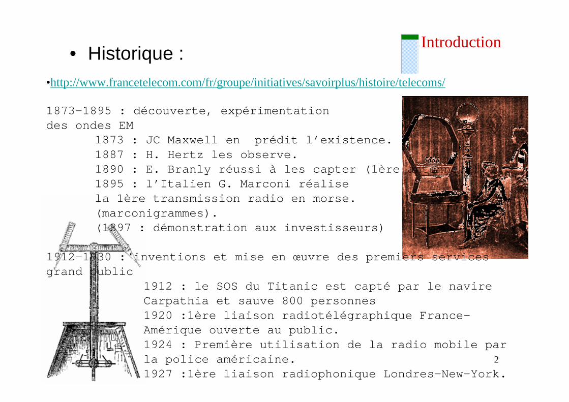
Introduction• Historique :
1873-1895 : découverte, expérimentation des ondes EM
1873 : JC Maxwell en prédit l’existence.1887 : H. Hertz les observe.1890 : E. Branly réussi à les capter (1ère antenne? ?).1895 : l’Italien G. Marconi réalise la 1ère transmission radio en morse. (marconigrammes). (1897 : démonstration aux investisseurs)
1912-1930 : inventions et mise en œuvre des premier s services grand public
1912 : le SOS du Titanic est capté par le navireCarpathia et sauve 800 personnes1920 :1ère liaison radiotélégraphique France-Amérique ouverte au public.1924 : Première utilisation de la radio mobile par la police américaine.1927 :1ère liaison radiophonique Londres-New-York.
•http://www.francetelecom.com/fr/groupe/initiatives/savoirplus/histoire/telecoms/
CIT
I -D
ept T
éléc
om
s -
INS
A L
yon
3
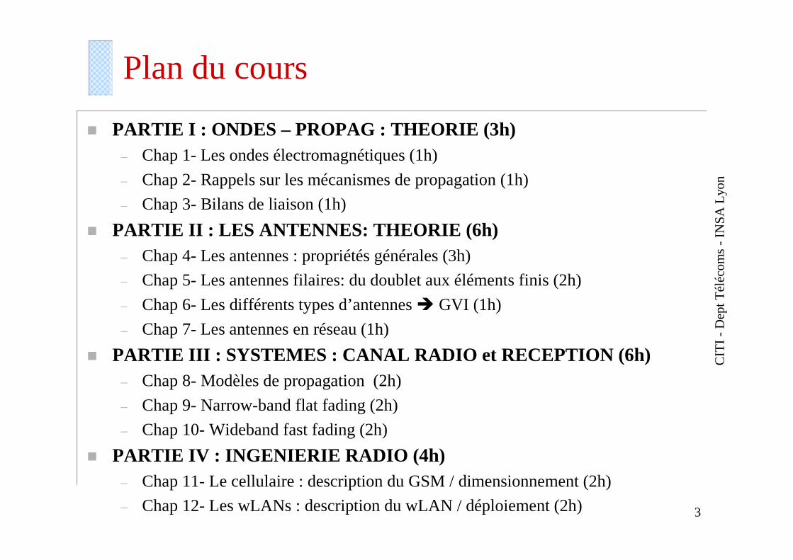
Plan du cours
� PARTIE I : ONDES – PROPAG : THEORIE (3h)– Chap 1- Les ondes électromagnétiques (1h)
– Chap 2- Rappels sur les mécanismes de propagation (1h)
– Chap 3- Bilans de liaison (1h)
� PARTIE II : LES ANTENNES: THEORIE (6h)– Chap 4- Les antennes : propriétés générales (3h)
– Chap 5- Les antennes filaires: du doublet aux éléments finis (2h)
– Chap 6- Les différents types d’antennes � GVI (1h)
– Chap 7- Les antennes en réseau (1h)
� PARTIE III : SYSTEMES : CANAL RADIO et RECEPTION (6h)– Chap 8- Modèles de propagation (2h)
– Chap 9- Narrow-band flat fading (2h)
– Chap 10- Wideband fast fading (2h)
� PARTIE IV : INGENIERIE RADIO (4h)– Chap 11- Le cellulaire : description du GSM / dimensionnement (2h)
– Chap 12- Les wLANs : description du wLAN / déploiement (2h)
CIT
I -D
ept T
éléc
om
s -
INS
A L
yon
4
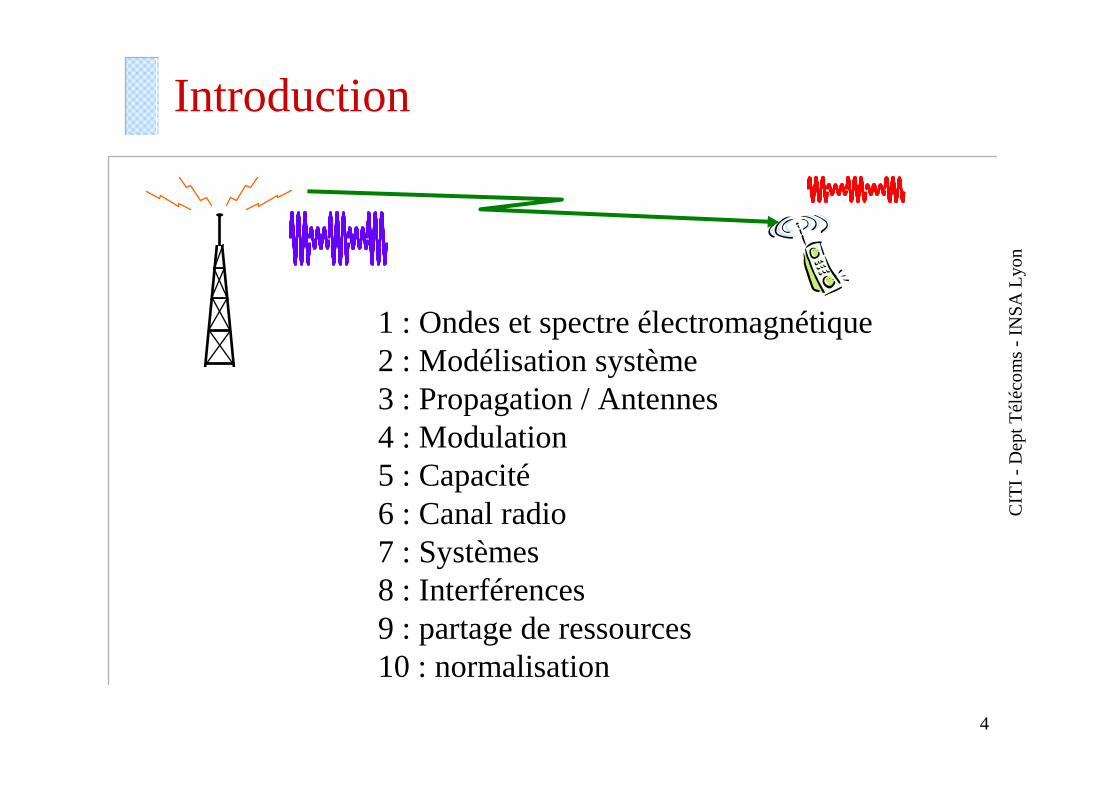
Introduction
1 : Ondes et spectre électromagnétique2 : Modélisation système3 : Propagation / Antennes4 : Modulation 5 : Capacité 6 : Canal radio7 : Systèmes8 : Interférences9 : partage de ressources10 : normalisation
CIT
I -D
ept T
éléc
om
s -
INS
A L
yon
5
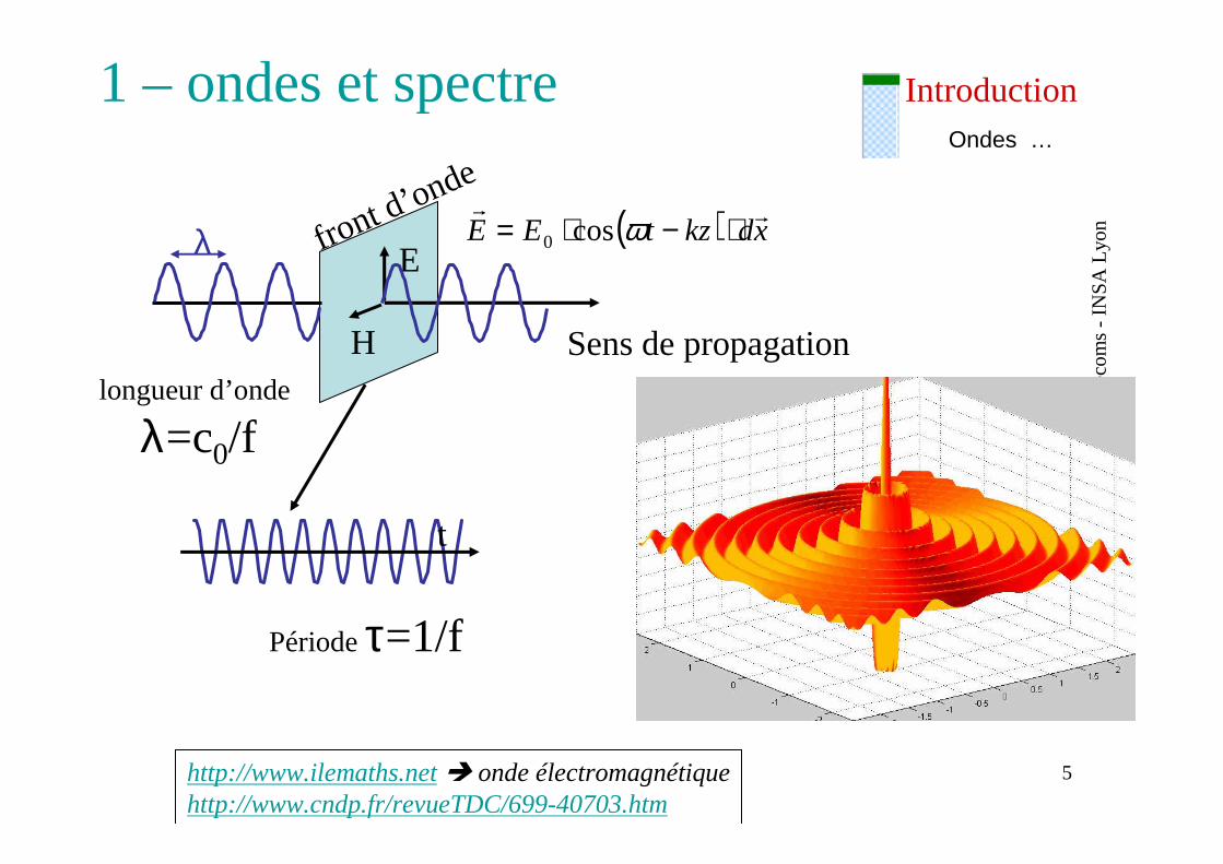
IntroductionOndes …
Sens de propagation
front d’onde
E
H
λ ( ) xdkztEErr
⋅−⋅= ωcos0
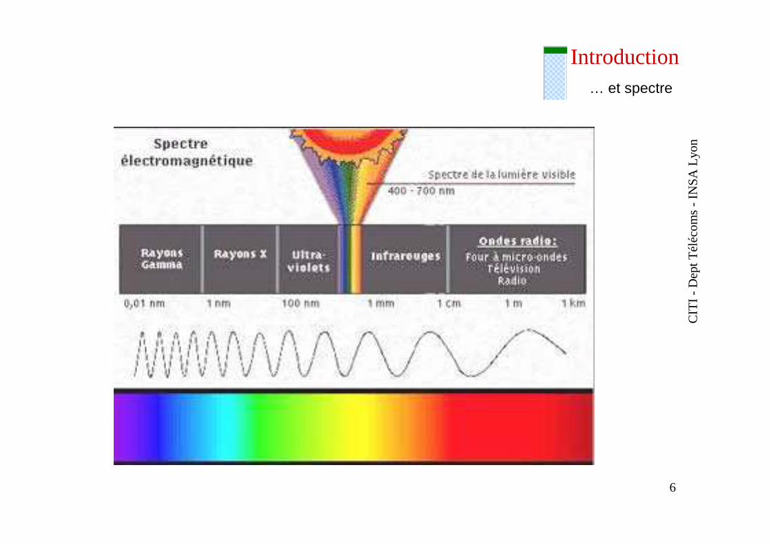
1 – ondes et spectre
longueur d’onde
λ=c0/f
t
Période τ=1/f
http://www.ilemaths.net� onde électromagnétiquehttp://www.cndp.fr/revueTDC/699-40703.htm
CIT
I -D
ept T
éléc
om
s -
INS
A L
yon
6
Introduction… et spectre
CIT
I -D
ept T
éléc
om
s -
INS
A L
yon
7
Introduction… et spectre
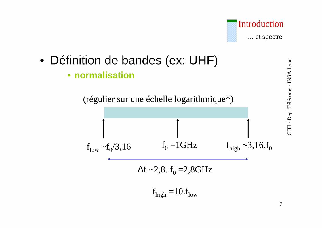
• Définition de bandes (ex: UHF)• normalisation
f0 =1GHzf low ~f0/3,16 fhigh ~3,16.f0
(régulier sur une échelle logarithmique*)
∆f ~2,8. f0 =2,8GHz
fhigh =10.flow
CIT
I -D
ept T
éléc
om
s -
INS
A L
yon
8
Introduction
120 dBm
100
80
60
40
20
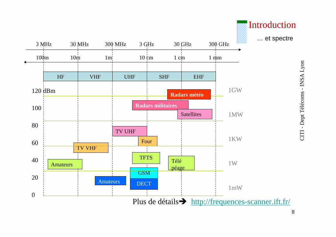
HF VHF UHF SHF EHF
TV VHF
Amateurs
Amateurs
GSM
TV UHF
Radars militaires
Satellites
Four
Télépéage
DECT
TFTS
0
1W
1mW
1MW
1KW
1GWRadars météo
… et spectre3 MHz
100m
30 MHz
10m
300 MHz
1m
3 GHz
10 cm
30 GHz
1 cm
300 GHz
1 mm
Plus de détails� http://frequences-scanner.ift.fr/
CIT
I -D
ept T
éléc
om
s -
INS
A L
yon
9
Introduction
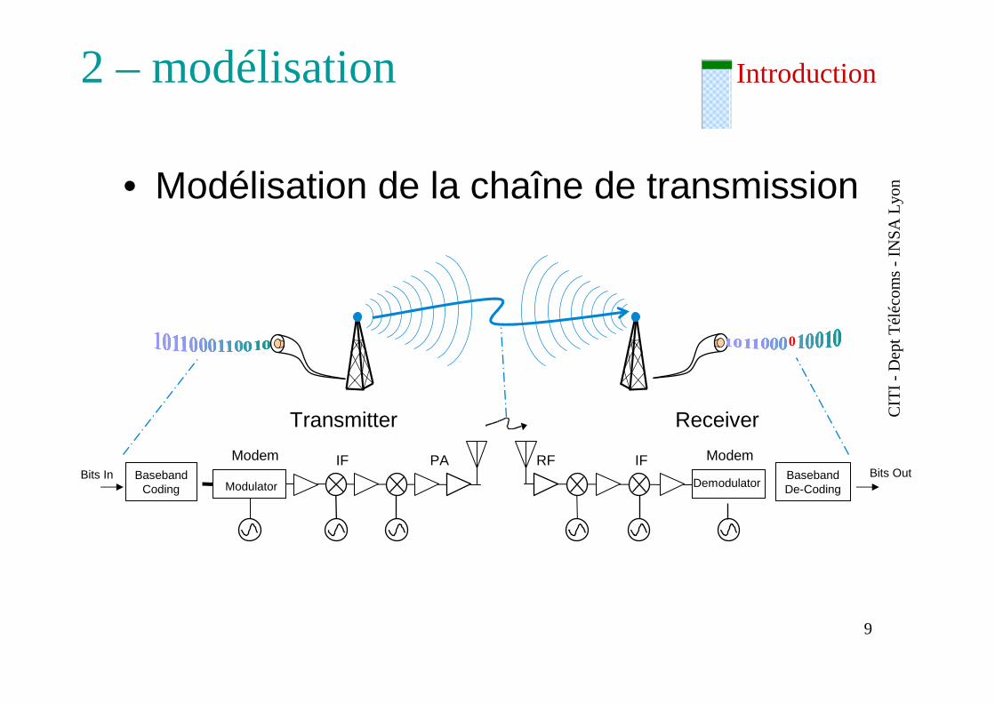
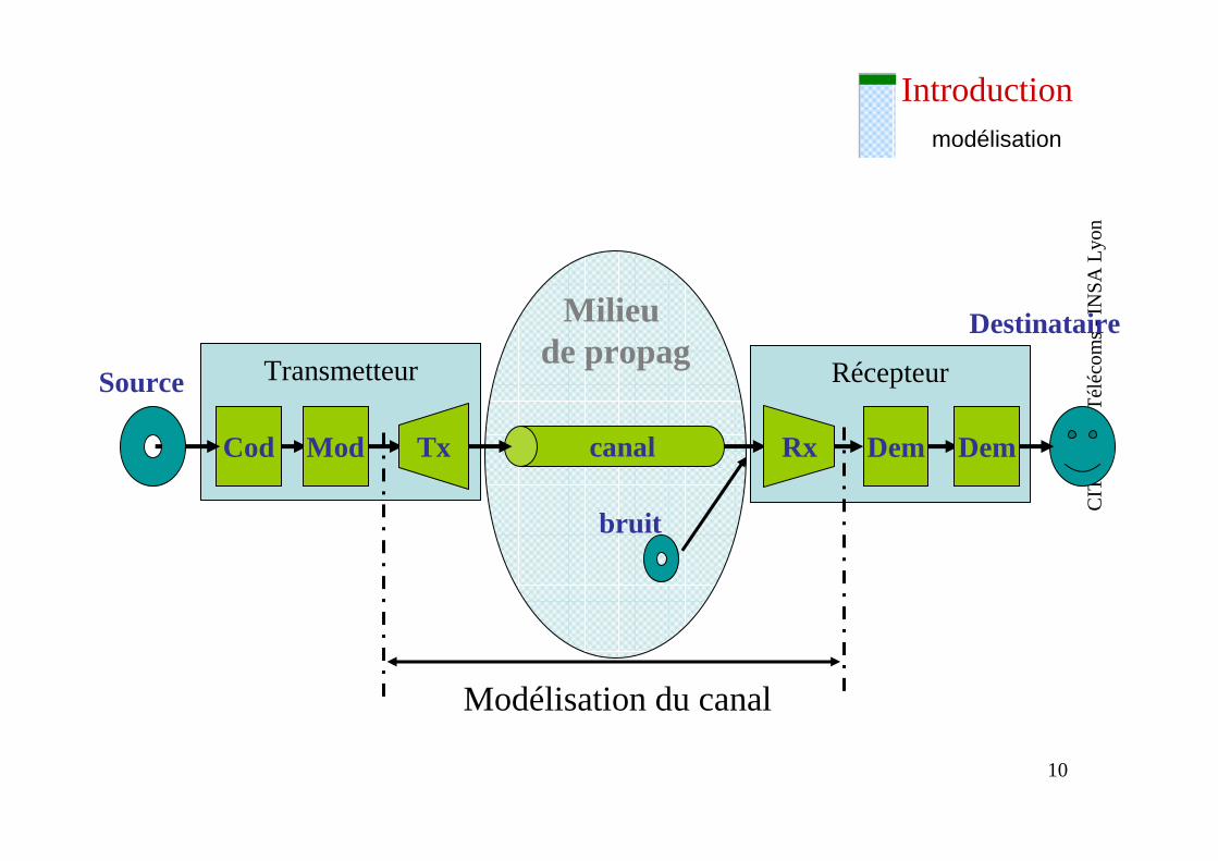
• Modélisation de la chaîne de transmission
2 – modélisation
0
ReceiverTransmitter
Modulator
Modem Modem
Demodulator
RF IFPAIFBaseband
CodingBasebandDe-Coding
Bits In Bits Out
CIT
I -D
ept T
éléc
om
s -
INS
A L
yon
10
Introduction
RécepteurTransmetteurSource
DestinataireMilieu de propag
Demcanal RxCod TxMod Dem
modélisation
bruit
Modélisation du canal
CIT
I -D
ept T
éléc
om
s -
INS
A L
yon
11
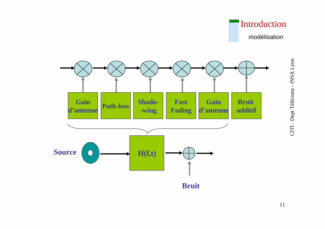
Introductionmodélisation
Gaind’antenne
Path-lossShado--wing
FastFading
Gaind’antenne
Bruit additif
H(f,t)Source
Bruit
CIT
I -D
ept T
éléc
om
s -
INS
A L
yon
12
IntroductionPropagation
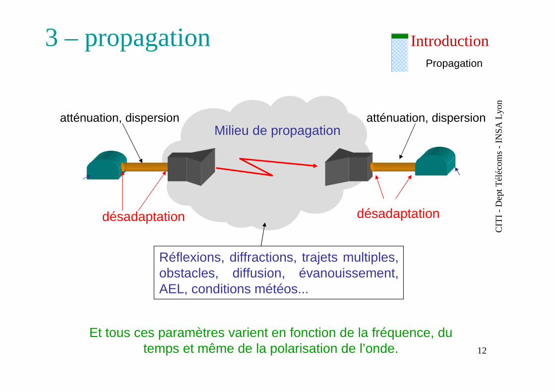
3 – propagation
désadaptation désadaptation
Milieu de propagation
Réflexions, diffractions, trajets multiples, obstacles, diffusion, évanouissement, AEL, conditions météos...
atténuation, dispersion atténuation, dispersion
Et tous ces paramètres varient en fonction de la fréquence, du temps et même de la polarisation de l’onde.
CIT
I -D
ept T
éléc
om
s -
INS
A L
yon
13
IntroductionPropagation
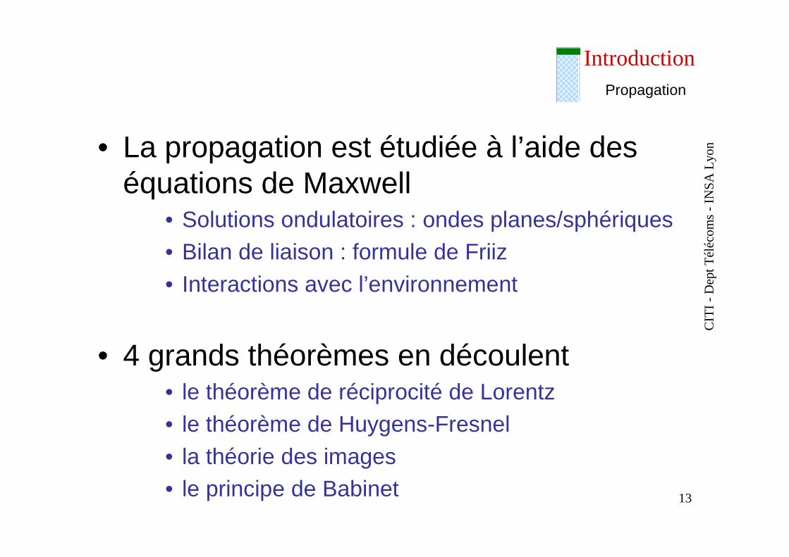
• La propagation est étudiée à l’aide des équations de Maxwell
• Solutions ondulatoires : ondes planes/sphériques• Bilan de liaison : formule de Friiz• Interactions avec l’environnement
• 4 grands théorèmes en découlent• le théorème de réciprocité de Lorentz• le théorème de Huygens-Fresnel• la théorie des images• le principe de Babinet
CIT
I -D
ept T
éléc
om
s -
INS
A L
yon
14
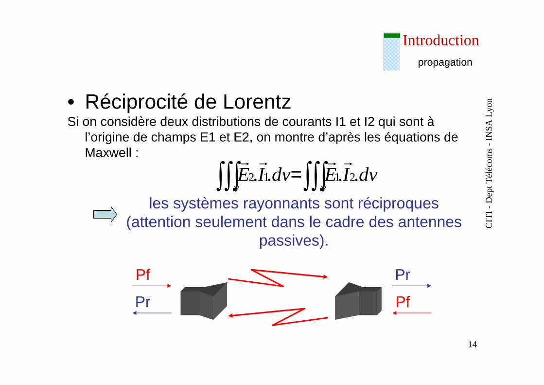
Introductionpropagation
• Réciprocité de LorentzSi on considère deux distributions de courants I1 et I2 qui sont à
l’origine de champs E1 et E2, on montre d’après les équations deMaxwell :
∫∫∫∫∫∫ =vv
dvIEdvIE .... 2112
rrrr
les systèmes rayonnants sont réciproques (attention seulement dans le cadre des antennes
passives).
Pf Pr
PfPr
CIT
I -D
ept T
éléc
om
s -
INS
A L
yon
15
IntroductionCanal radio
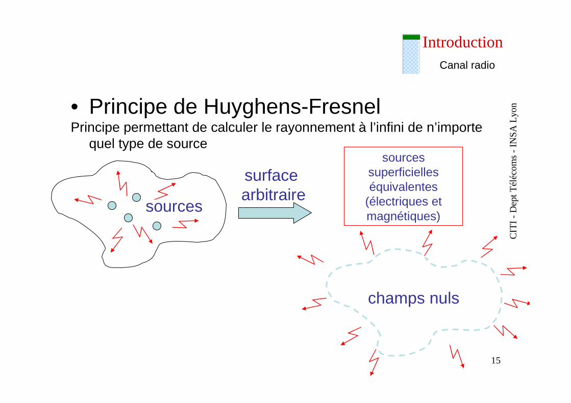
• Principe de Huyghens-FresnelPrincipe permettant de calculer le rayonnement à l’infini de n’importe
quel type de source
sources
surface arbitraire
champs nuls
sources superficielles équivalentes
(électriques et magnétiques)
CIT
I -D
ept T
éléc
om
s -
INS
A L
yon
16
IntroductionCanal radio
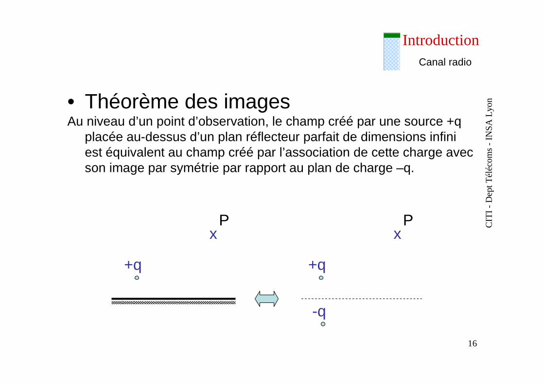
• Théorème des imagesAu niveau d’un point d’observation, le champ créé par une source +q
placée au-dessus d’un plan réflecteur parfait de dimensions infini est équivalent au champ créé par l’association de cette charge avec son image par symétrie par rapport au plan de charge –q.
+q
Px
+q
Px
-q
CIT
I -D
ept T
éléc
om
s -
INS
A L
yon
17
IntroductionCanal radio
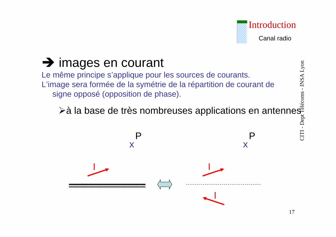
� images en courantLe même principe s’applique pour les sources de courants.L’image sera formée de la symétrie de la répartition de courant de
signe opposé (opposition de phase).
Px
Px
I I
I
�à la base de très nombreuses applications en antennes
CIT
I -D
ept T
éléc
om
s -
INS
A L
yon
18
IntroductionCanal radio
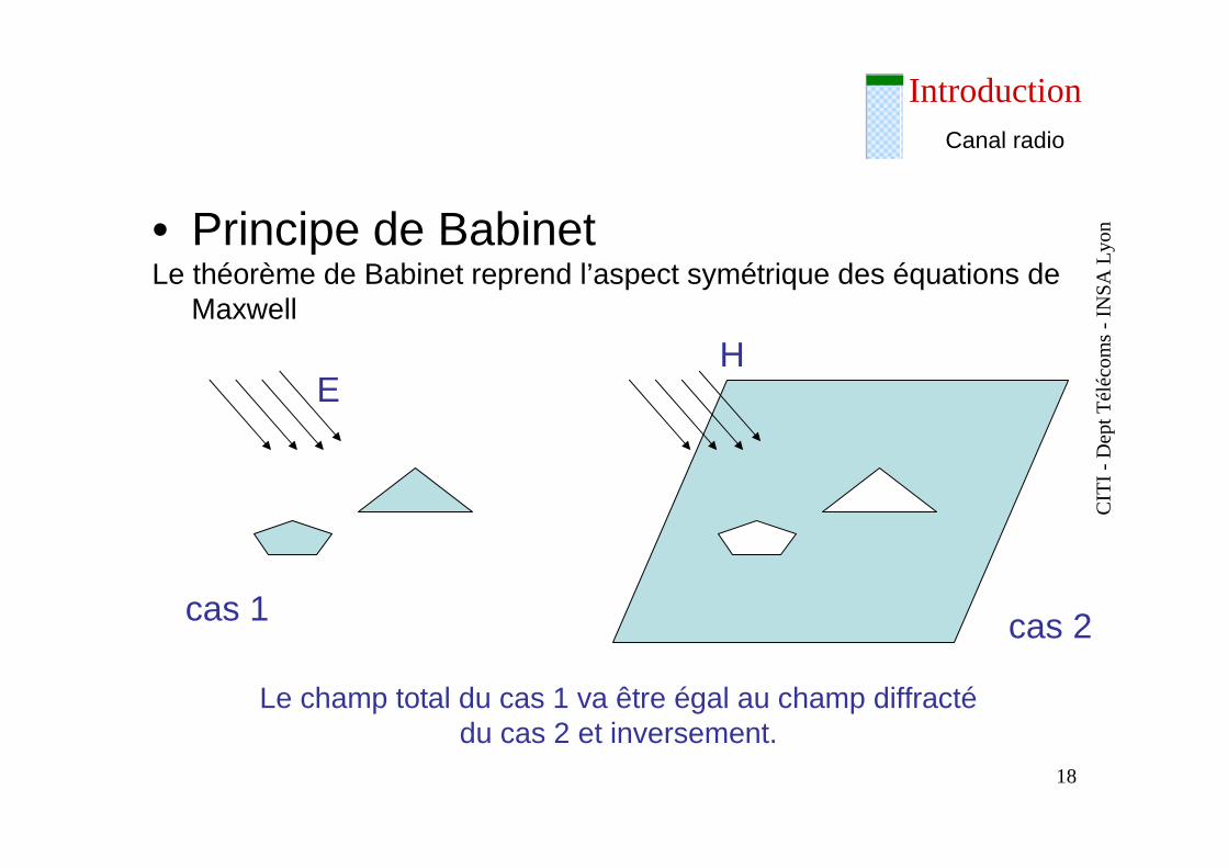
• Principe de BabinetLe théorème de Babinet reprend l’aspect symétrique des équations de
Maxwell
EH
cas 1 cas 2
Le champ total du cas 1 va être égal au champ diffracté du cas 2 et inversement.
CIT
I -D
ept T
éléc
om
s -
INS
A L
yon
19
IntroductionCanal radio
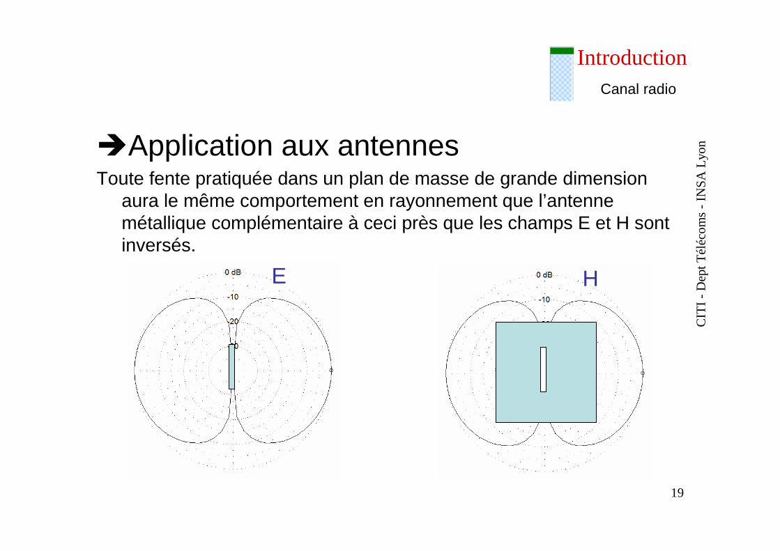
�Application aux antennesToute fente pratiquée dans un plan de masse de grande dimension
aura le même comportement en rayonnement que l’antenne métallique complémentaire à ceci près que les champs E et H sontinversés.
E H
CIT
I -D
ept T
éléc
om
s -
INS
A L
yon
20
Introduction
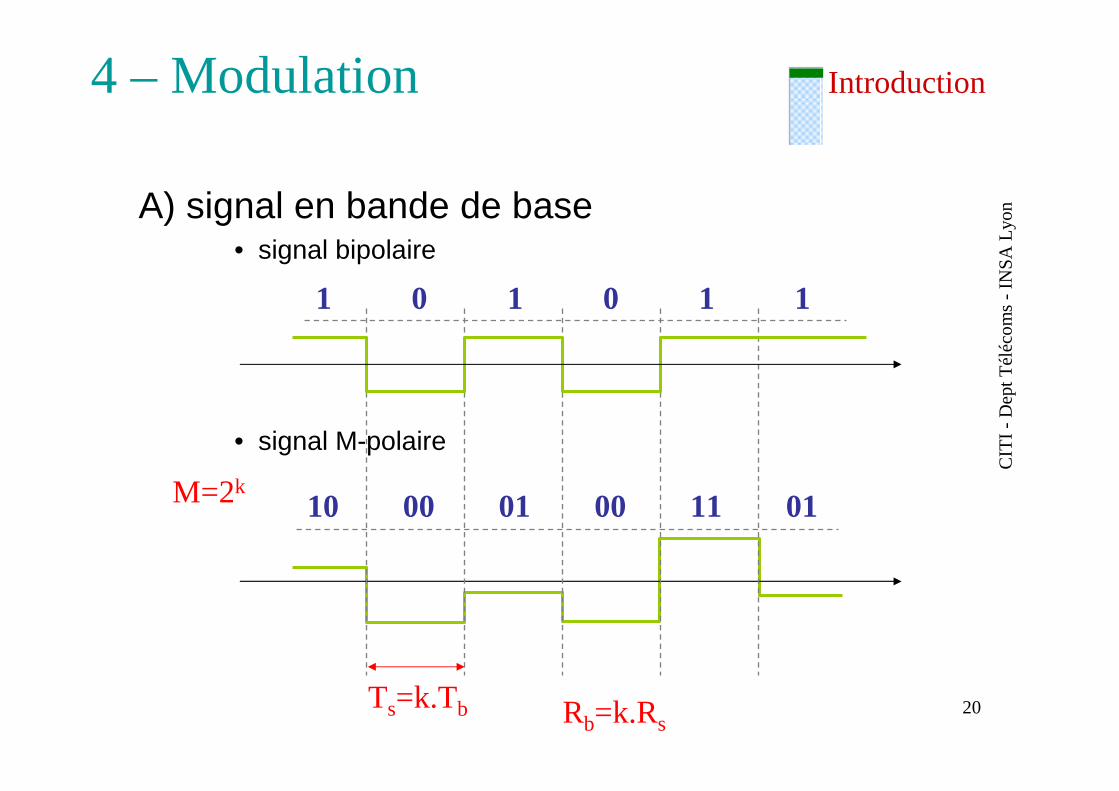
1 0 1 0 1 1
10 00 01 00 11 01
Ts=k.Tb
M=2k
Rb=k.Rs
4 – Modulation
A) signal en bande de base • signal bipolaire
• signal M-polaire
CIT
I -D
ept T
éléc
om
s -
INS
A L
yon
21
Introduction
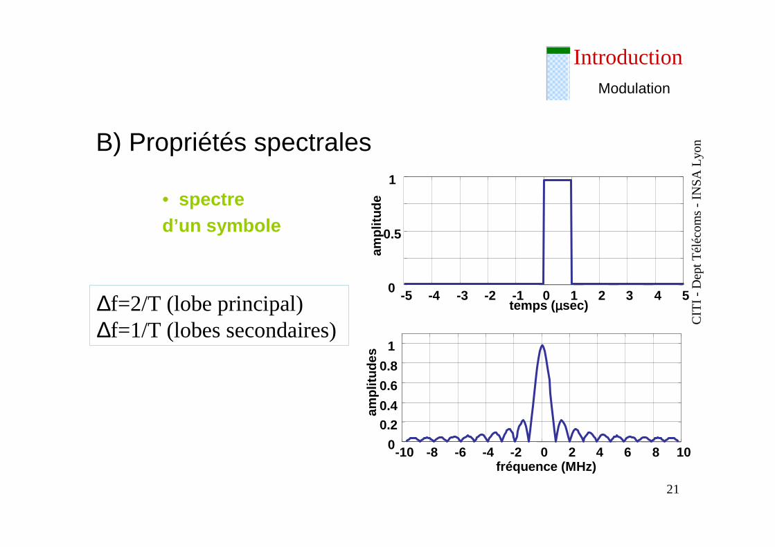
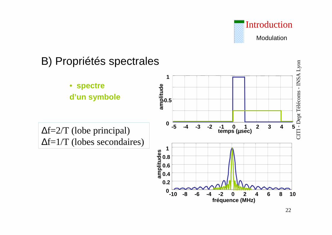
∆f=2/T (lobe principal)∆f=1/T (lobes secondaires)
Modulation
B) Propriétés spectrales
• spectre d’un symbole
-10 -8 -6 -4 -2 0 2 4 6 8 100
0.20.4
0.6
0.8
1
fréquence (MHz)
ampl
itude
s
-5 -4 -3 -2 -1 0 1 2 3 4 50
0.5
1
temps ( µµµµsec)
ampl
itude
CIT
I -D
ept T
éléc
om
s -
INS
A L
yon
22
Introduction
-10 -8 -6 -4 -2 0 2 4 6 8 100
0.20.4
0.6
0.8
1
fréquence (MHz)
ampl
itude
s
-5 -4 -3 -2 -1 0 1 2 3 4 50
0.5
1
temps ( µµµµsec)
ampl
itude
∆f=2/T (lobe principal)∆f=1/T (lobes secondaires)
Modulation
B) Propriétés spectrales
• spectre d’un symbole
CIT
I -D
ept T
éléc
om
s -
INS
A L
yon
23
Introduction
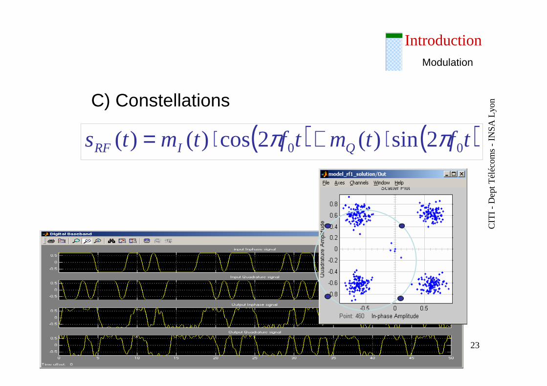
( ) ( )tftmtftmts QIRF 00 2sin)(2cos)()( ππ ⋅+⋅=
Modulation
C) Constellations
CIT
I -D
ept T
éléc
om
s -
INS
A L
yon
24
Introduction
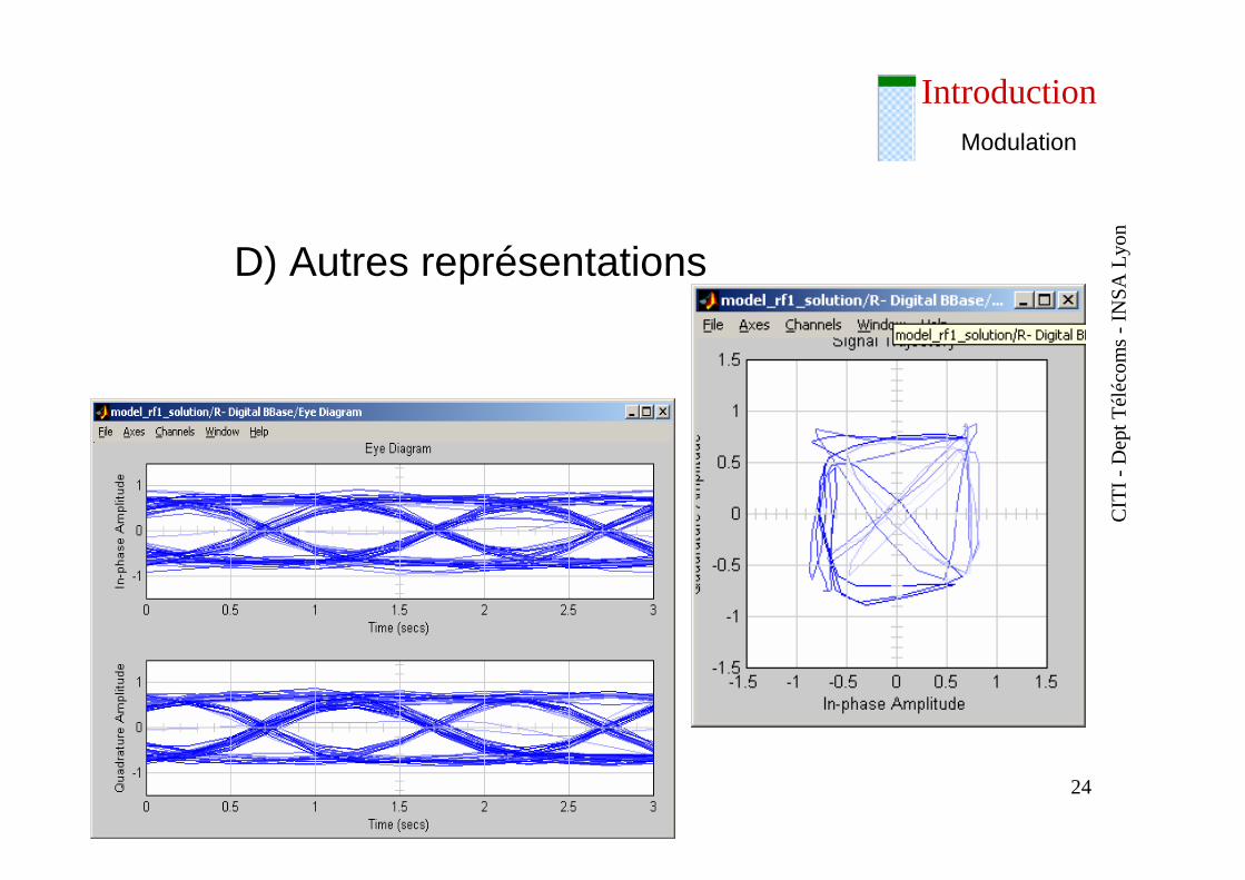
D) Autres représentations
Modulation
CIT
I -D
ept T
éléc
om
s -
INS
A L
yon
25
Introduction
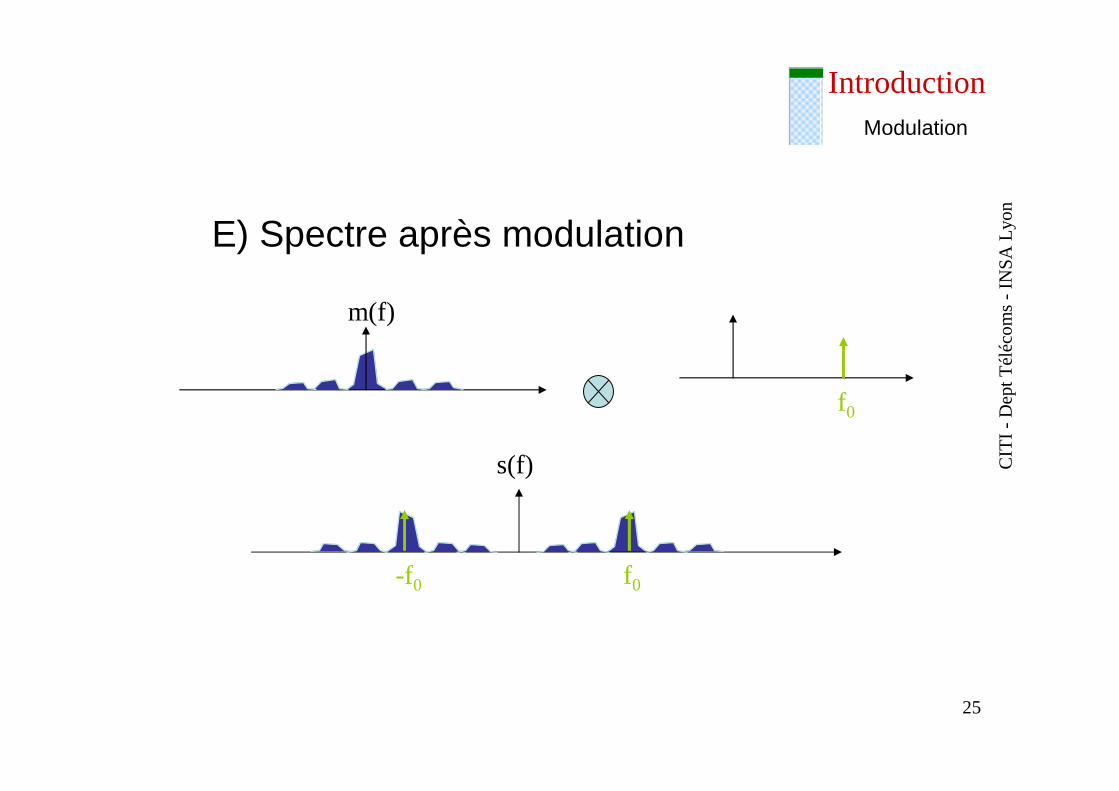
E) Spectre après modulation
m(f)
f0
s(f)
f0-f0
Modulation
CIT
I -D
ept T
éléc
om
s -
INS
A L
yon
26
Introduction
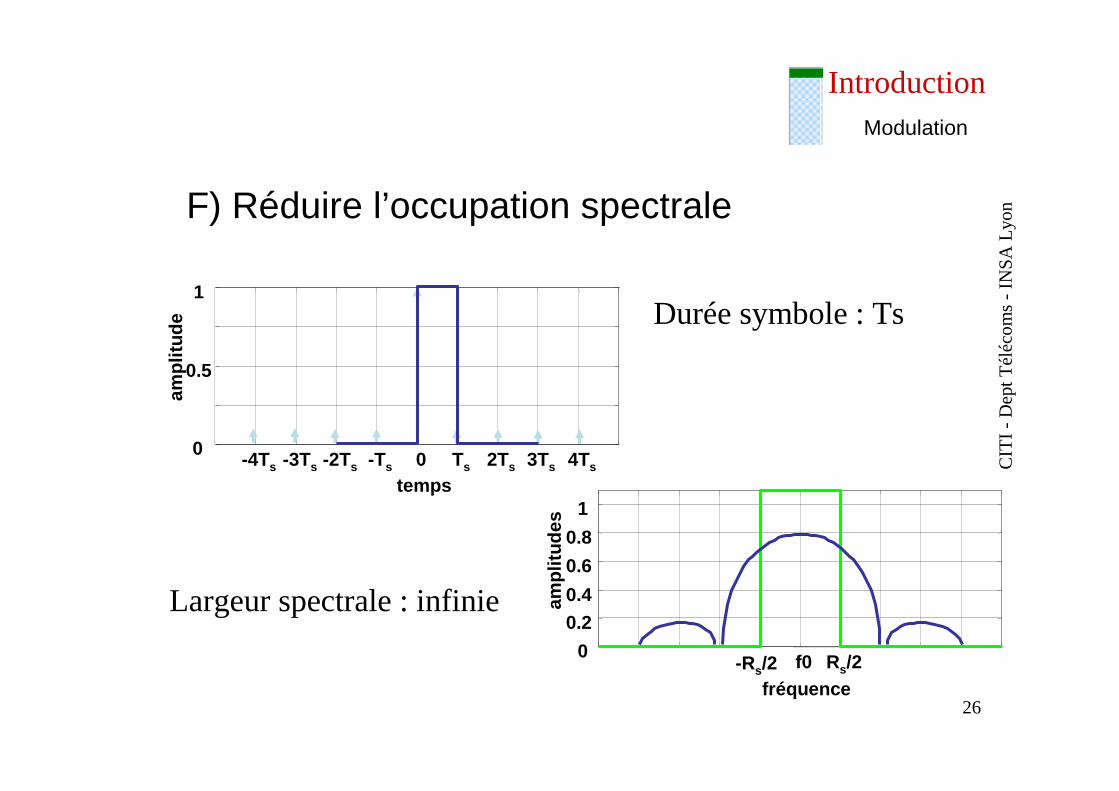
F) Réduire l’occupation spectrale
-Rs/2 f0 Rs/20
0.20.4
0.6
0.8
1
fréquence
ampl
itude
s
-4Ts -3Ts -2Ts -Ts 0 Ts 2Ts 3Ts 4Ts0
0.5
1
temps
ampl
itude
Durée symbole : Ts
Largeur spectrale : infinie
Modulation
CIT
I -D
ept T
éléc
om
s -
INS
A L
yon
27
Introduction
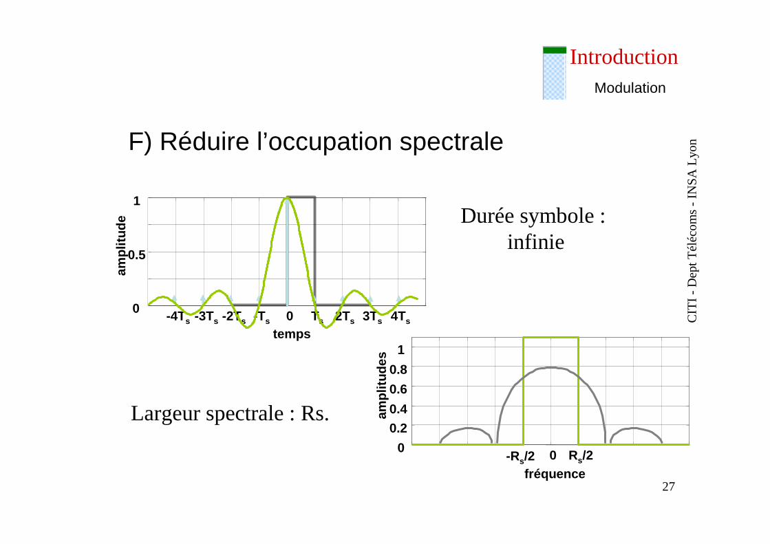
F) Réduire l’occupation spectrale
-4Ts -3Ts -2Ts -Ts 0 Ts 2Ts 3Ts 4Ts0
0.5
1
temps
ampl
itude
-Rs/2 0 Rs/20
0.20.4
0.6
0.8
1
fréquence
ampl
itude
s
Durée symbole : infinie
Largeur spectrale : Rs.
Modulation
CIT
I -D
ept T
éléc
om
s -
INS
A L
yon
28
Introduction
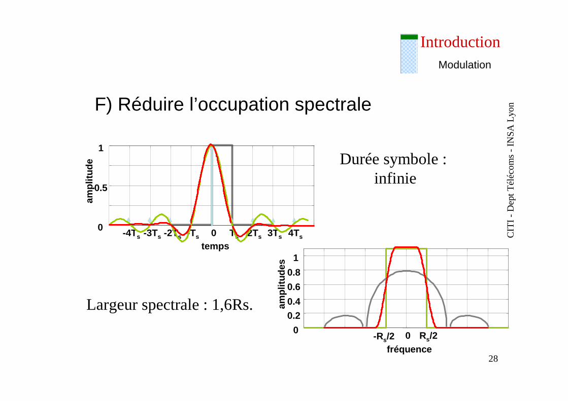
F) Réduire l’occupation spectrale
-4Ts -3Ts -2Ts -Ts 0 Ts 2Ts 3Ts 4Ts0
0.5
1
temps
ampl
itude
-Rs/2 0 Rs/20
0.20.4
0.6
0.8
1
fréquence
ampl
itude
s
Durée symbole : infinie
Largeur spectrale : 1,6Rs.
Modulation
CIT
I -D
ept T
éléc
om
s -
INS
A L
yon
29
Introduction
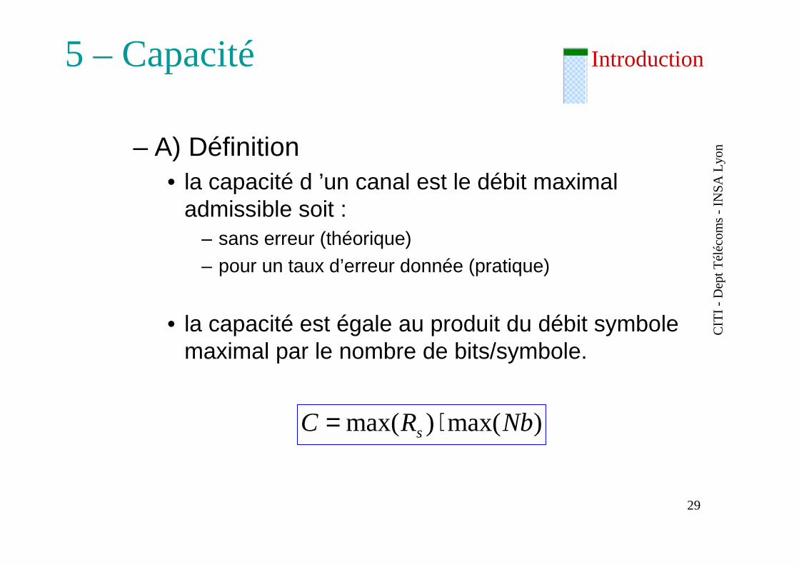
– A) Définition• la capacité d ’un canal est le débit maximal
admissible soit : – sans erreur (théorique) – pour un taux d’erreur donnée (pratique)
• la capacité est égale au produit du débit symbole maximal par le nombre de bits/symbole.
)max()max( NbRC s ⋅=
5 – Capacité
CIT
I -D
ept T
éléc
om
s -
INS
A L
yon
30
Introduction
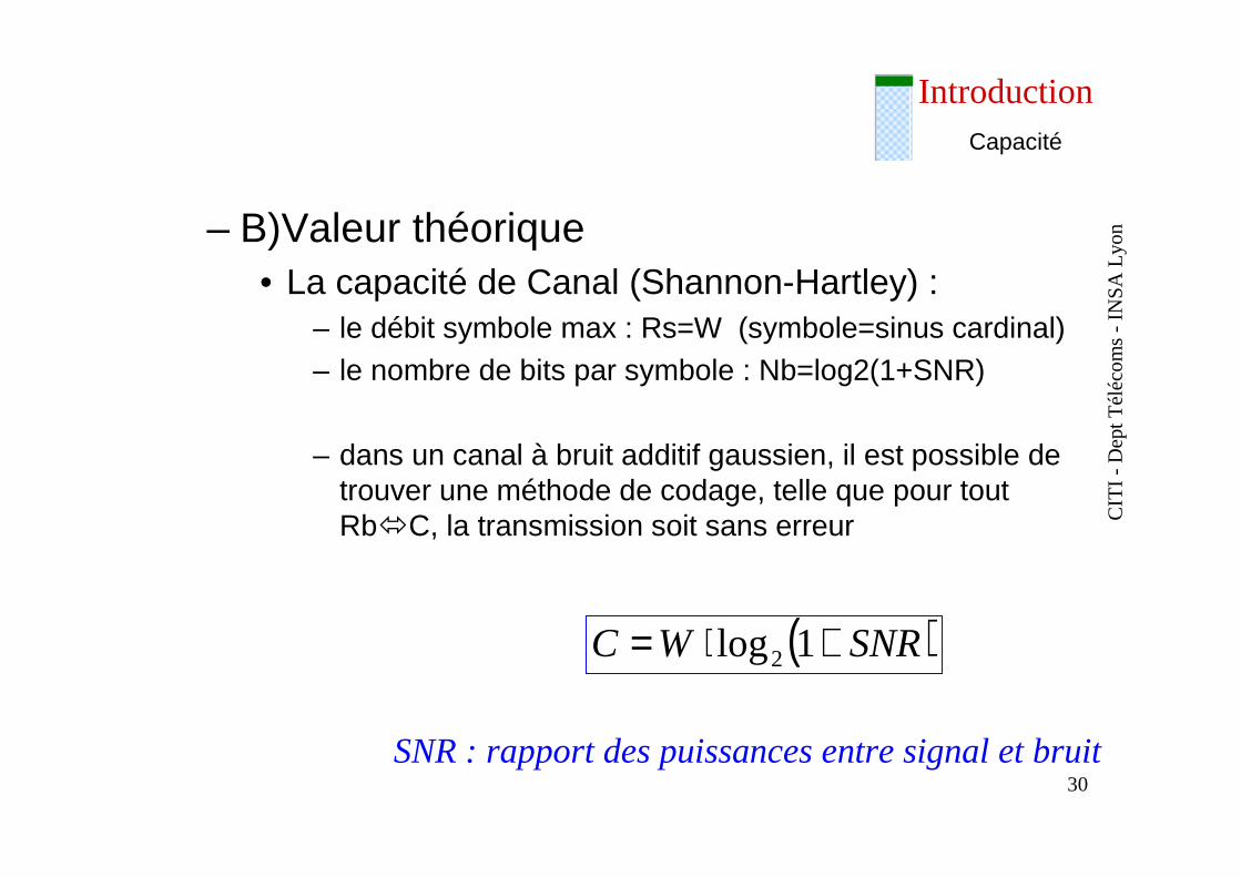
– B)Valeur théorique• La capacité de Canal (Shannon-Hartley) :
– le débit symbole max : Rs=W (symbole=sinus cardinal)– le nombre de bits par symbole : Nb=log2(1+SNR)
– dans un canal à bruit additif gaussien, il est possible de trouver une méthode de codage, telle que pour tout Rb�C, la transmission soit sans erreur
( )SNRWC +⋅= 1log2
SNR : rapport des puissances entre signal et bruit
Capacité
CIT
I -D
ept T
éléc
om
s -
INS
A L
yon
31
Introduction
– C)Valeur expérimentale
• La capacité de Canal pour un système donné :– le débit symbole max : Rs ~1,6.W (dépend de la qualité
de la modulation, et des contraintes imposées en terme de largeur spectrale : bande à -3dB, -10dB, etc...)
– le nombre de bits par symbole dépend du taux d ’erreur acceptable : Nb=f(SNR) (cf. courbes précédentes)
– La capacité est donnée par le produit des 2.
Capacité
CIT
I -D
ept T
éléc
om
s -
INS
A L
yon
32
Introduction
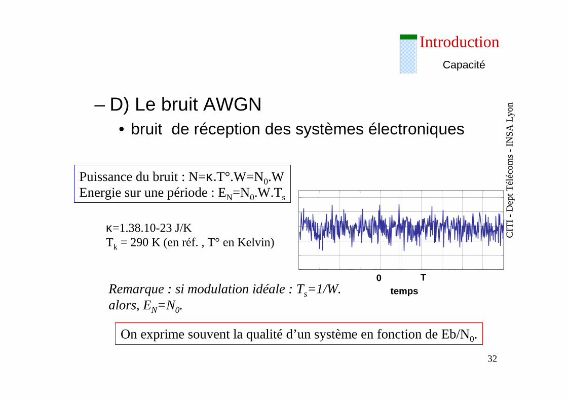
– D) Le bruit AWGN• bruit de réception des systèmes électroniques
Puissance du bruit : N=κ.T°.W=N0.WEnergie sur une période : EN=N0.W.Ts
0 TtempsRemarque : si modulation idéale : Ts=1/W.
alors, EN=N0.
On exprime souvent la qualité d’un système en fonction de Eb/N0.
κ=1.38.10-23 J/K Tk = 290 K (en réf. , T° en Kelvin)
Capacité
CIT
I -D
ept T
éléc
om
s -
INS
A L
yon
33
Introduction
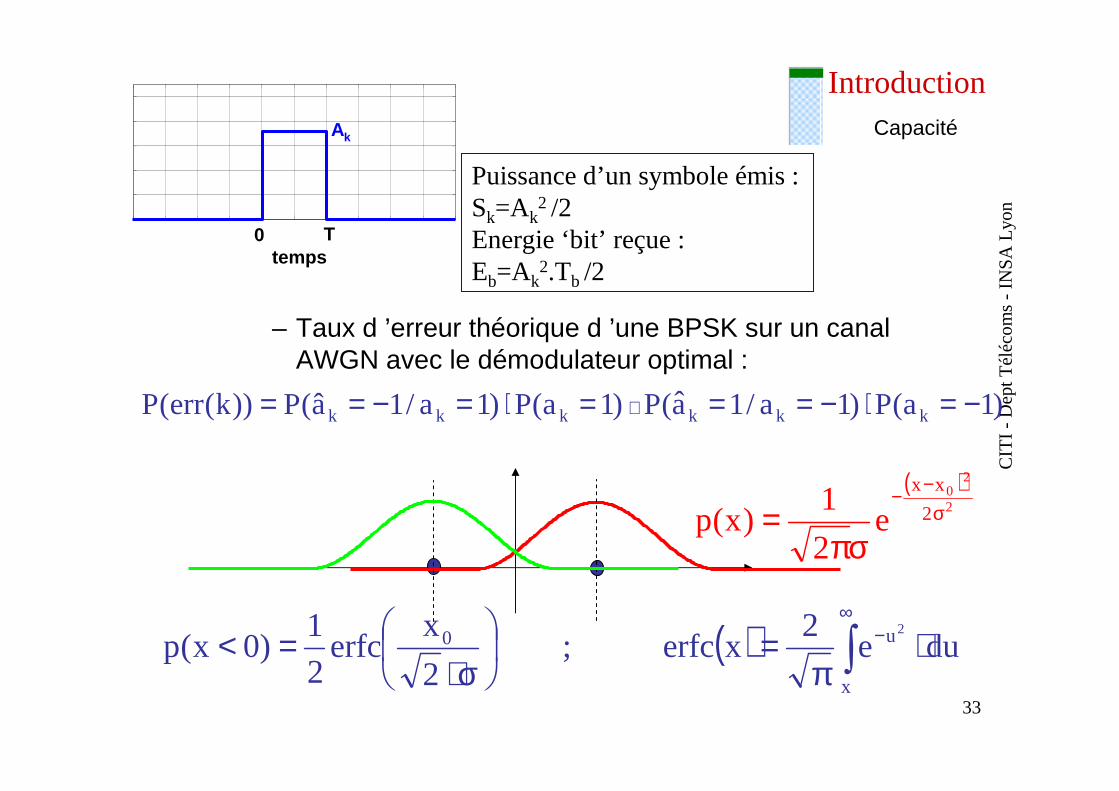
Puissance d’un symbole émis : Sk=Ak
2 /2Energie ‘bit’ reçue : Eb=Ak
2.Tb /2
0 Ttemps
Ak Capacité
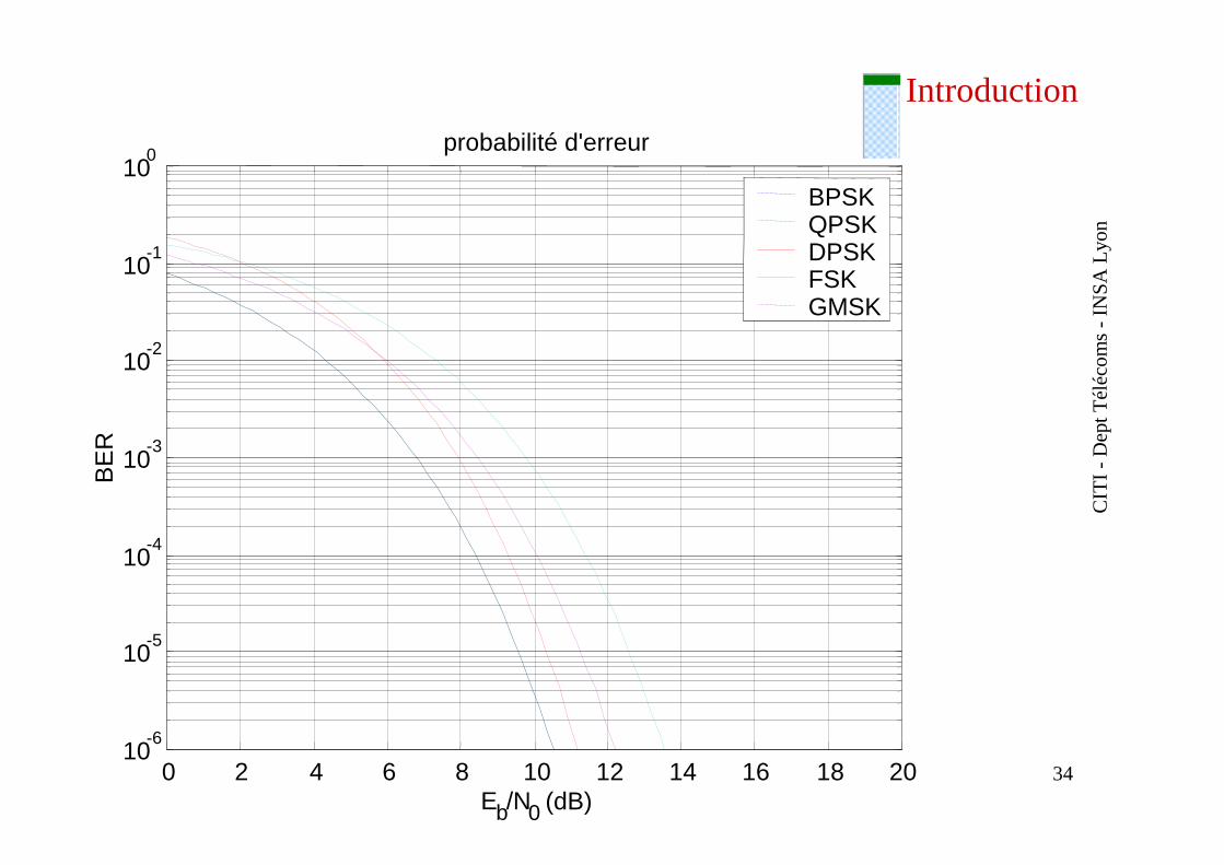
– Taux d ’erreur théorique d ’une BPSK sur un canal AWGN avec le démodulateur optimal :
( )2
20
2
xx
e2
1)x(p σ
−−
σπ=
)1a(P)1a/1a(P)1a(P)1a/1â(P))k(err(P kkkkkk −=⋅−===⋅=−== +
( ) ∫∞
− ⋅π
=
σ⋅=<
x
u0 due2
xerfc;2
xerfc
2
1)0x(p
2
CIT
I -D
ept T
éléc
om
s -
INS
A L
yon
34
Introduction
0 2 4 6 8 10 12 14 16 18 2010
-6
10-5
10-4
10-3
10-2
10-1
100
Eb/N0 (dB)
BE
R
probabilité d'erreur
BPSKQPSKDPSKFSK GMSK
CIT
I -D
ept T
éléc
om
s -
INS
A L
yon
35
Introduction
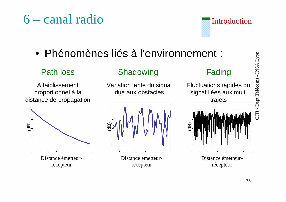
• Phénomènes liés à l’environnement :
6 – canal radio
Distance émetteur-récepteur
(dB
)
Path loss
Affaiblissement proportionnel à la
distance de propagation
Shadowing
Distance émetteur-récepteur
(dB
)
Variation lente du signal due aux obstacles
Fading
Distance émetteur-récepteur
(dB
)
Fluctuations rapides du signal liées aux multi
trajets
CIT
I -D
ept T
éléc
om
s -
INS
A L
yon
36
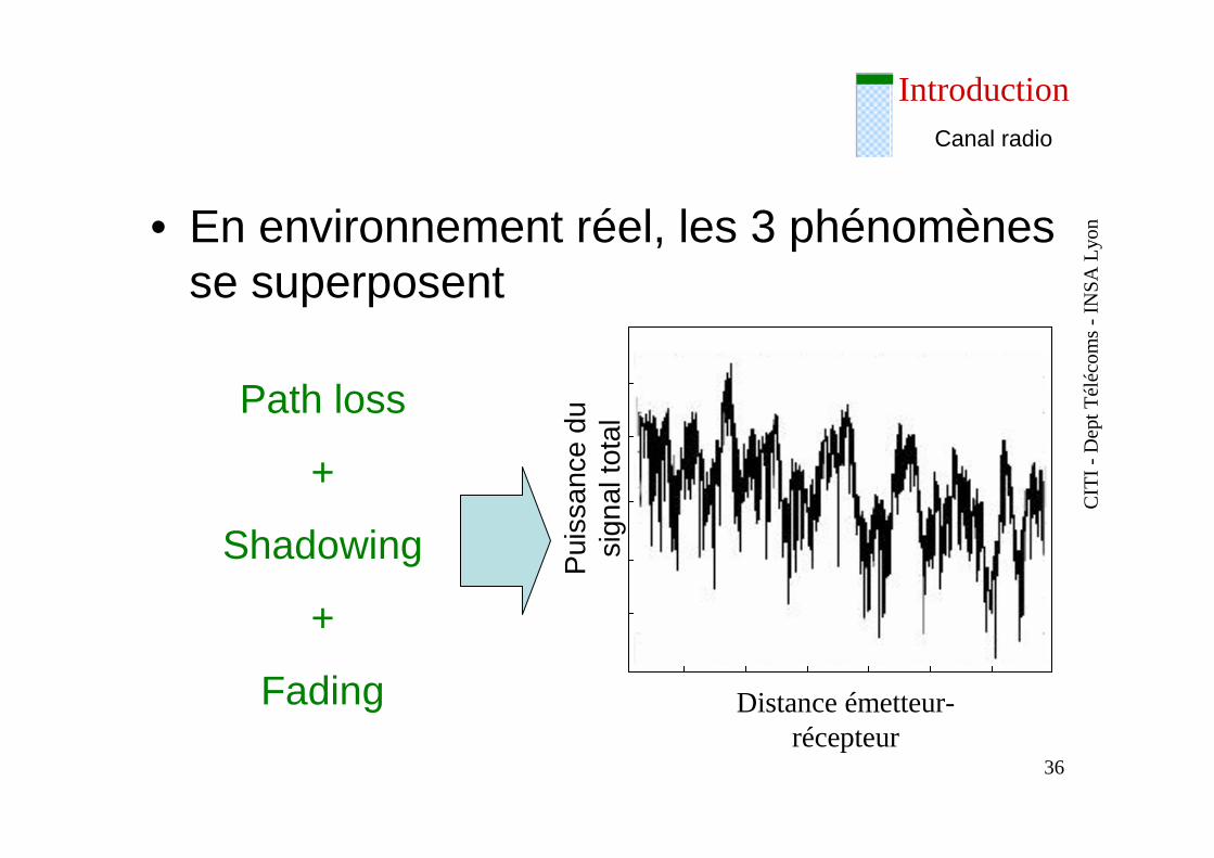
Introduction
Distance émetteur-récepteur
Pui
ssan
ce d
u si
gnal
tota
lPath loss
+
Shadowing
+
Fading
Canal radio
• En environnement réel, les 3 phénomènes se superposent
CIT
I -D
ept T
éléc
om
s -
INS
A L
yon
37
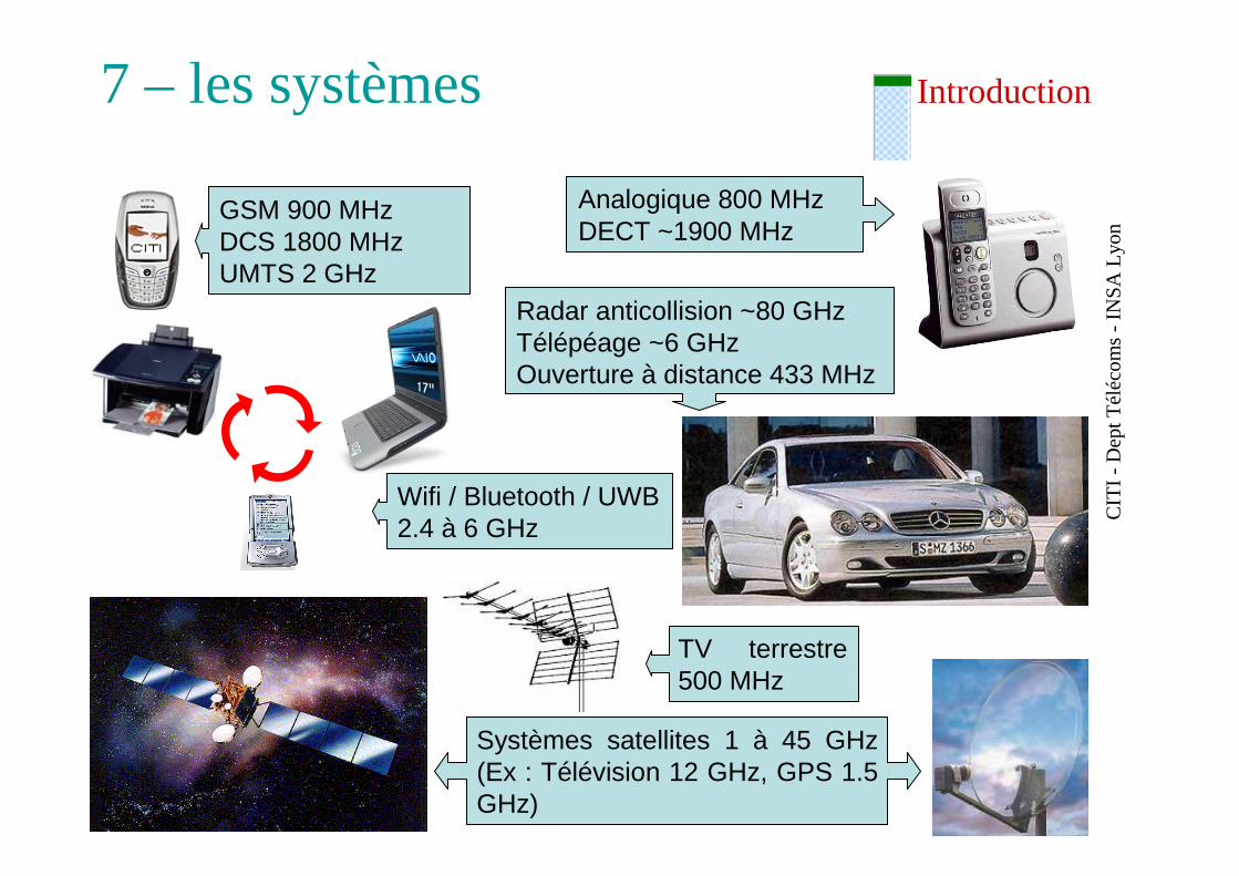
Introduction7 – les systèmes
Analogique 800 MHzDECT ~1900 MHz
Radar anticollision ~80 GHzTélépéage ~6 GHzOuverture à distance 433 MHz
GSM 900 MHzDCS 1800 MHzUMTS 2 GHz
Systèmes satellites 1 à 45 GHz (Ex : Télévision 12 GHz, GPS 1.5 GHz)
TV terrestre 500 MHz
Wifi / Bluetooth / UWB2.4 à 6 GHz
CIT
I -D
ept T
éléc
om
s -
INS
A L
yon
38
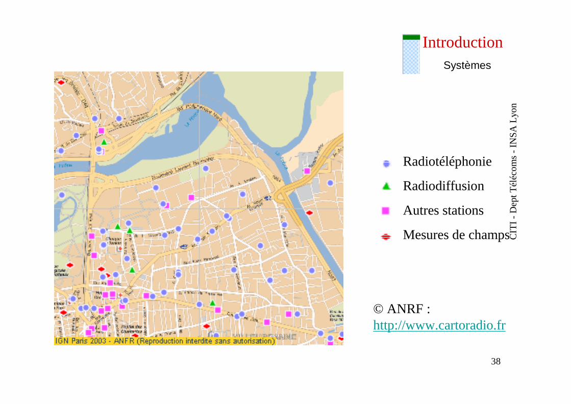
Introduction
Mesures de champs
Autres stations
Radiodiffusion
Radiotéléphonie
© ANRF :http://www.cartoradio.fr
Systèmes
CIT
I -D
ept T
éléc
om
s -
INS
A L
yon
39
IntroductionSystèmes
• La diffusion• La liaison point à point• L’accès fixe• Les radio-mobiles• Les réseaux cellulaires
CIT
I -D
ept T
éléc
om
s -
INS
A L
yon
40
IntroductionSystèmes
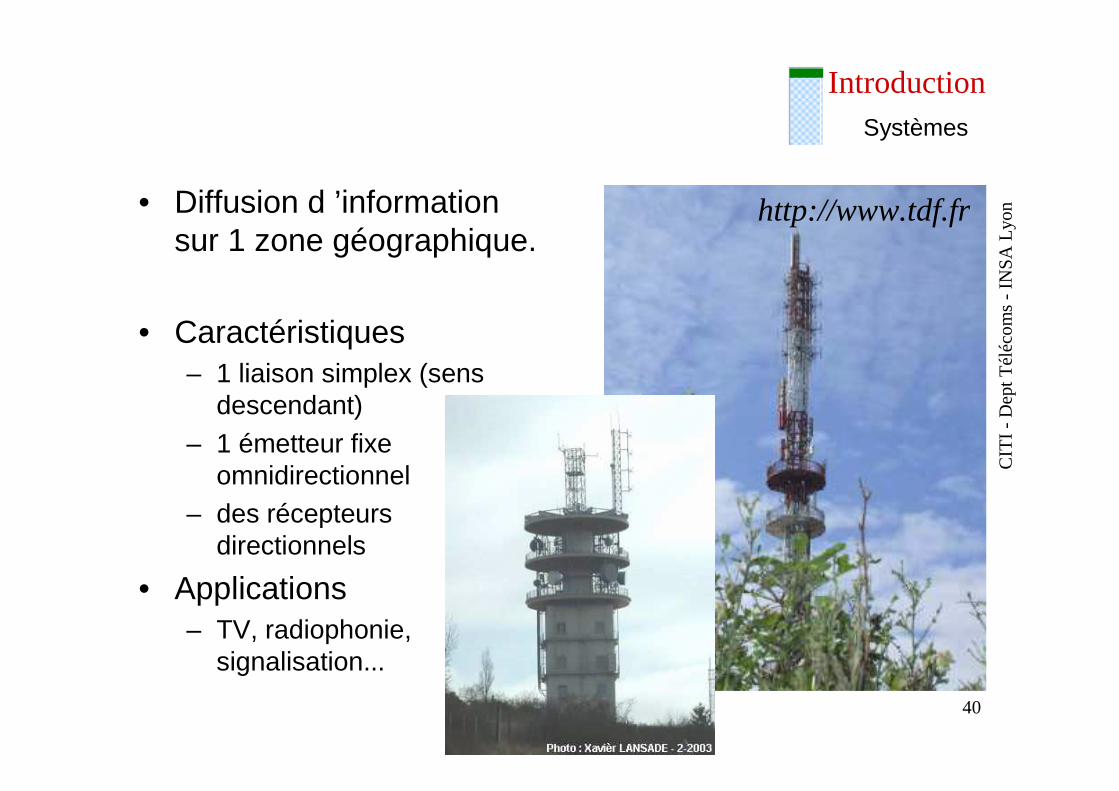
• Diffusion d ’information sur 1 zone géographique.
• Caractéristiques – 1 liaison simplex (sens
descendant)– 1 émetteur fixe
omnidirectionnel– des récepteurs
directionnels
• Applications– TV, radiophonie,
signalisation...
http://www.tdf.fr
CIT
I -D
ept T
éléc
om
s -
INS
A L
yon
41
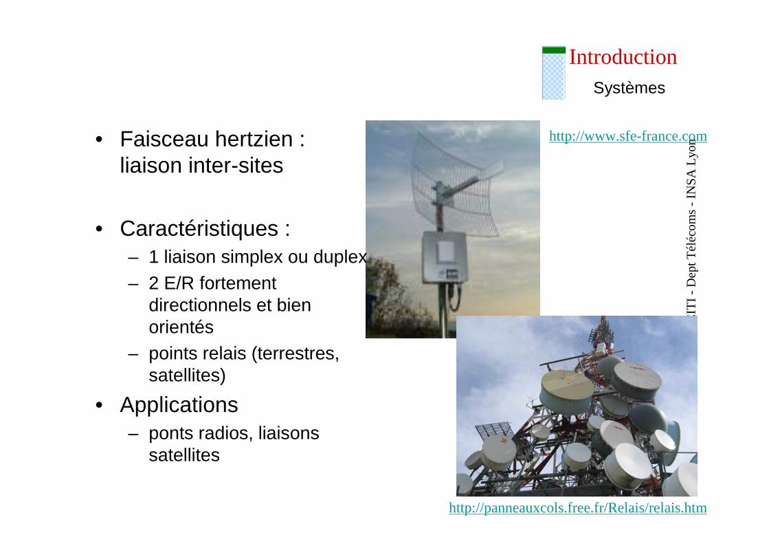
IntroductionSystèmes
• Faisceau hertzien : liaison inter-sites
• Caractéristiques :– 1 liaison simplex ou duplex– 2 E/R fortement
directionnels et bien orientés
– points relais (terrestres, satellites)
• Applications– ponts radios, liaisons
satellites
http://www.sfe-france.com
http://panneauxcols.free.fr/Relais/relais.htm
CIT
I -D
ept T
éléc
om
s -
INS
A L
yon
42
IntroductionSystèmes
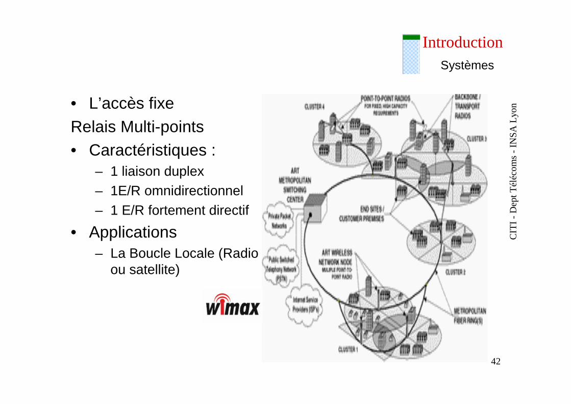
• L’accès fixeRelais Multi-points• Caractéristiques :
– 1 liaison duplex– 1E/R omnidirectionnel– 1 E/R fortement directif
• Applications– La Boucle Locale (Radio
ou satellite)
CIT
I -D
ept T
éléc
om
s -
INS
A L
yon
43
IntroductionSystèmes
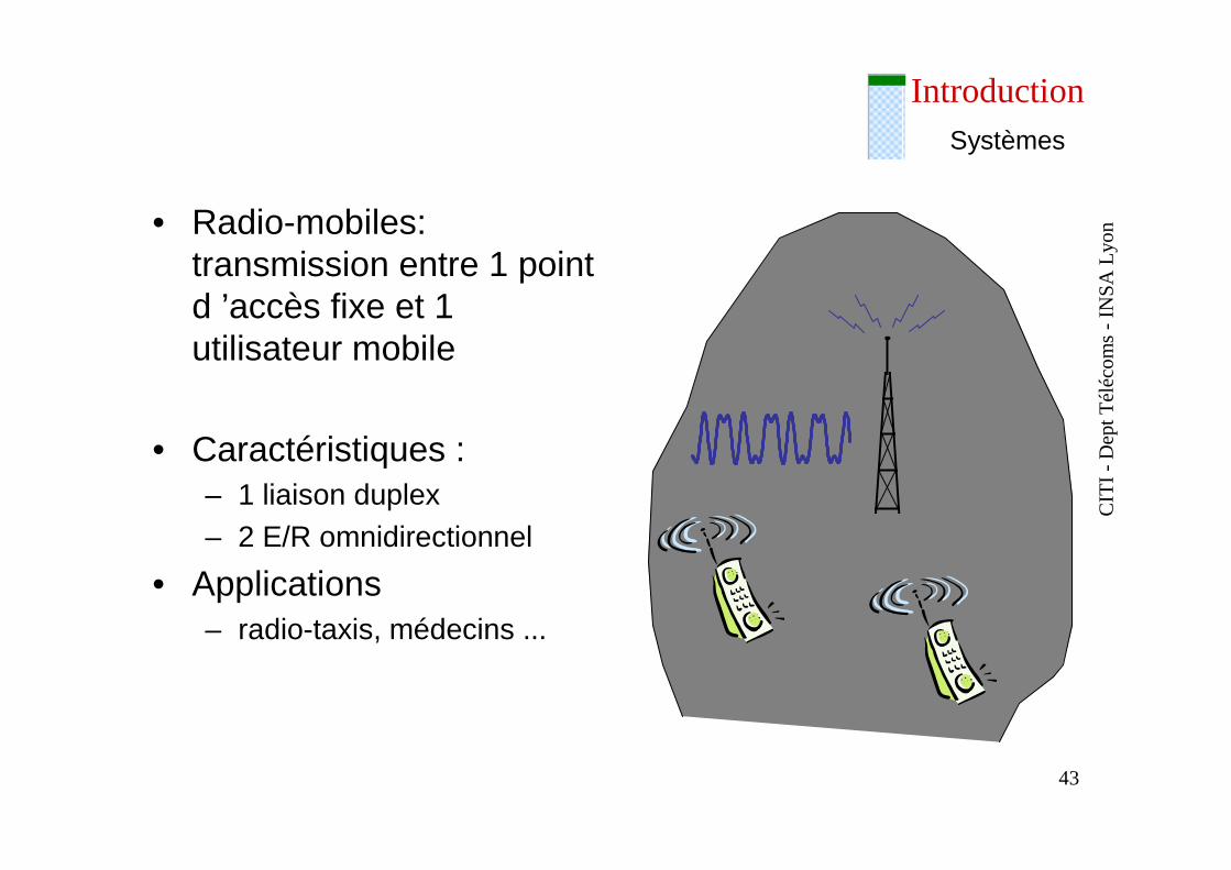
• Radio-mobiles: transmission entre 1 point d ’accès fixe et 1 utilisateur mobile
• Caractéristiques :– 1 liaison duplex– 2 E/R omnidirectionnel
• Applications– radio-taxis, médecins ...
CIT
I -D
ept T
éléc
om
s -
INS
A L
yon
44
IntroductionSystèmes
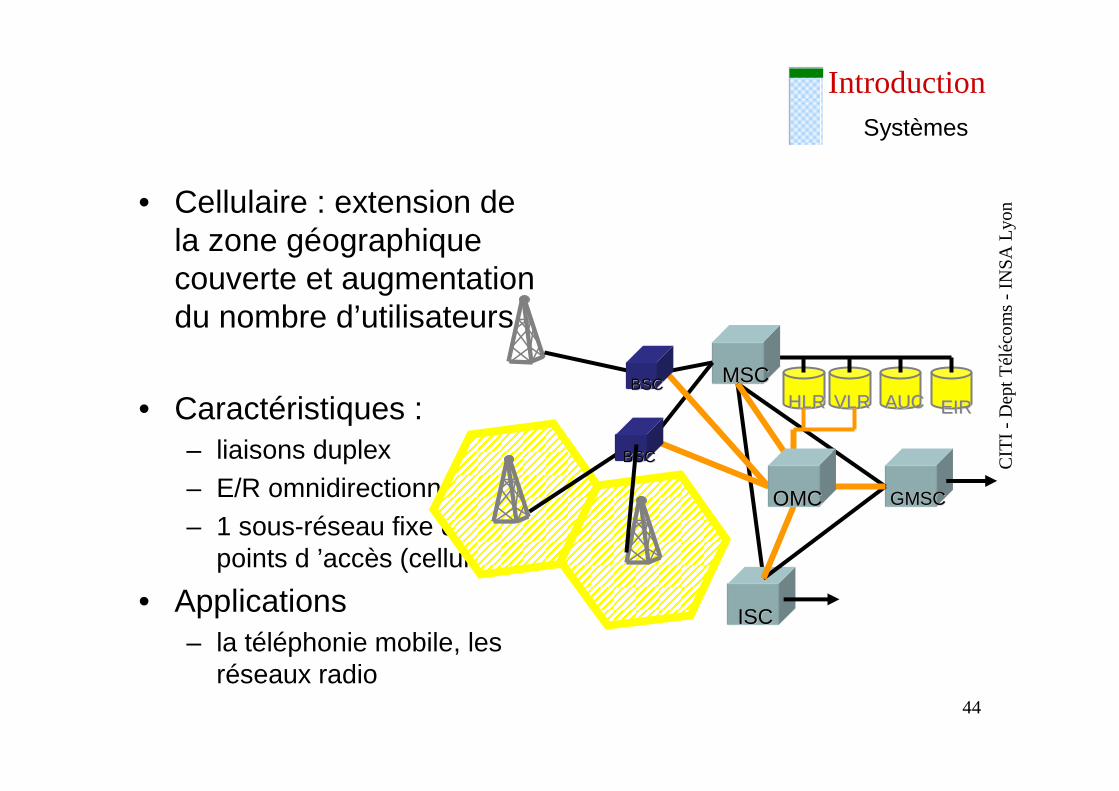
• Cellulaire : extension de la zone géographique couverte et augmentation du nombre d’utilisateurs
• Caractéristiques :– liaisons duplex– E/R omnidirectionnel– 1 sous-réseau fixe de
points d ’accès (cellules)
• Applications– la téléphonie mobile, les
réseaux radio
EIREIRVLRVLRHLRHLR AUCAUC
GMSCGMSC
ISCISC
MSCMSC
OMCOMC
BSCBSC
BSCBSC
CIT
I -D
ept T
éléc
om
s -
INS
A L
yon
45
Introduction
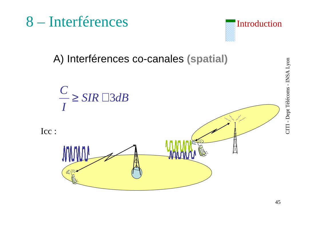
A) Interférences co-canales (spatial)
dBSIRI
C3+≥
Icc :
8 – Interférences
CIT
I -D
ept T
éléc
om
s -
INS
A L
yon
46
Introduction
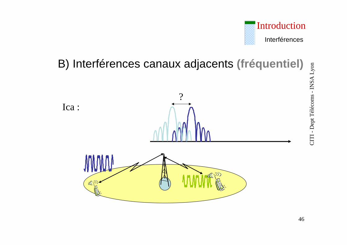
B) Interférences canaux adjacents (fréquentiel)
Ica : ?
Interférences
CIT
I -D
ept T
éléc
om
s -
INS
A L
yon
47
Introduction
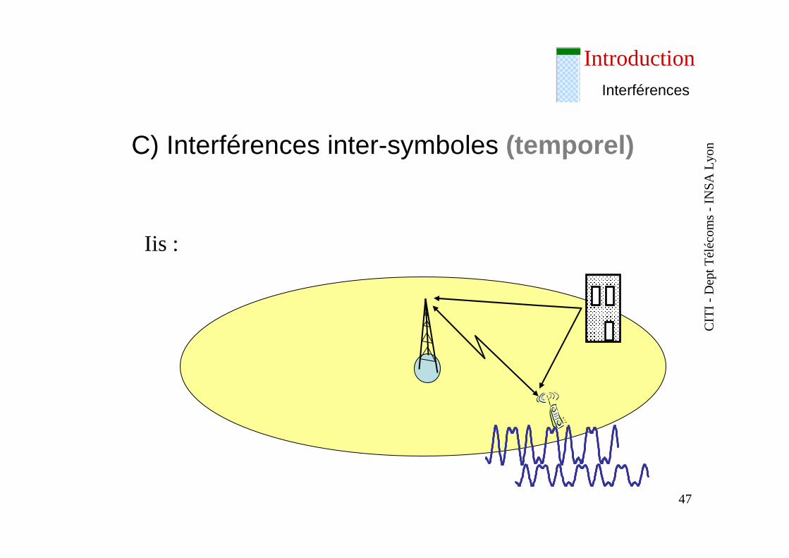
C) Interférences inter-symboles (temporel)
Iis :
Interférences
CIT
I -D
ept T
éléc
om
s -
INS
A L
yon
48
Introduction
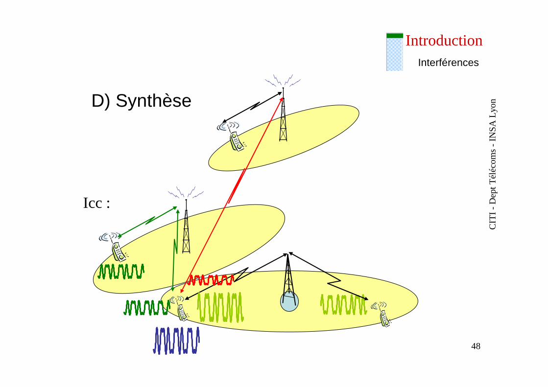
D) Synthèse
Icc :
Interférences
CIT
I -D
ept T
éléc
om
s -
INS
A L
yon
49
Introduction
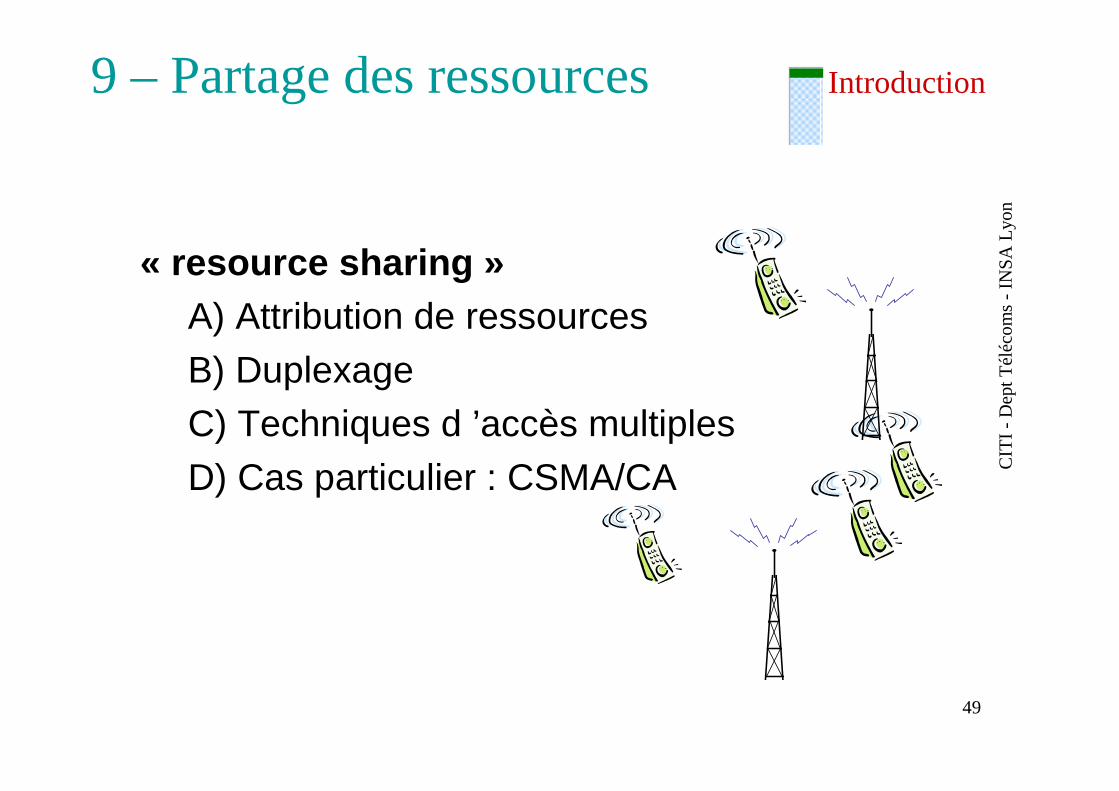
« resource sharing »A) Attribution de ressources
B) DuplexageC) Techniques d ’accès multiples
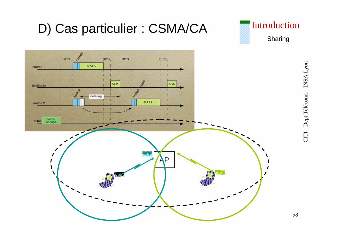
D) Cas particulier : CSMA/CA
9 – Partage des ressources
CIT
I -D
ept T
éléc
om
s -
INS
A L
yon
50
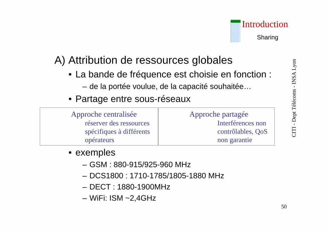
Introduction
A) Attribution de ressources globales• La bande de fréquence est choisie en fonction :
– de la portée voulue, de la capacité souhaitée…
• Partage entre sous-réseaux
• exemples– GSM : 880-915/925-960 MHz – DCS1800 : 1710-1785/1805-1880 MHz– DECT : 1880-1900MHz– WiFi: ISM ~2,4GHz
Sharing
Approche centralisée réserver des ressources spécifiques à différents opérateurs
Approche partagéeInterférences non contrôlables, QoSnon garantie
CIT
I -D
ept T
éléc
om
s -
INS
A L
yon
51
IntroductionSharing
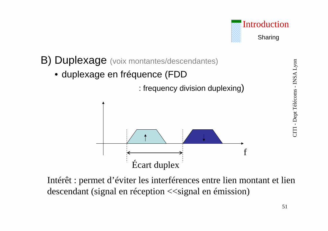
B) Duplexage (voix montantes/descendantes)
• duplexage en fréquence (FDD : frequency division duplexing)
fÉcart duplex
Intérêt : permet d’éviter les interférences entre lien montant et lien descendant (signal en réception <<signal en émission)
CIT
I -D
ept T
éléc
om
s -
INS
A L
yon
52
Introduction
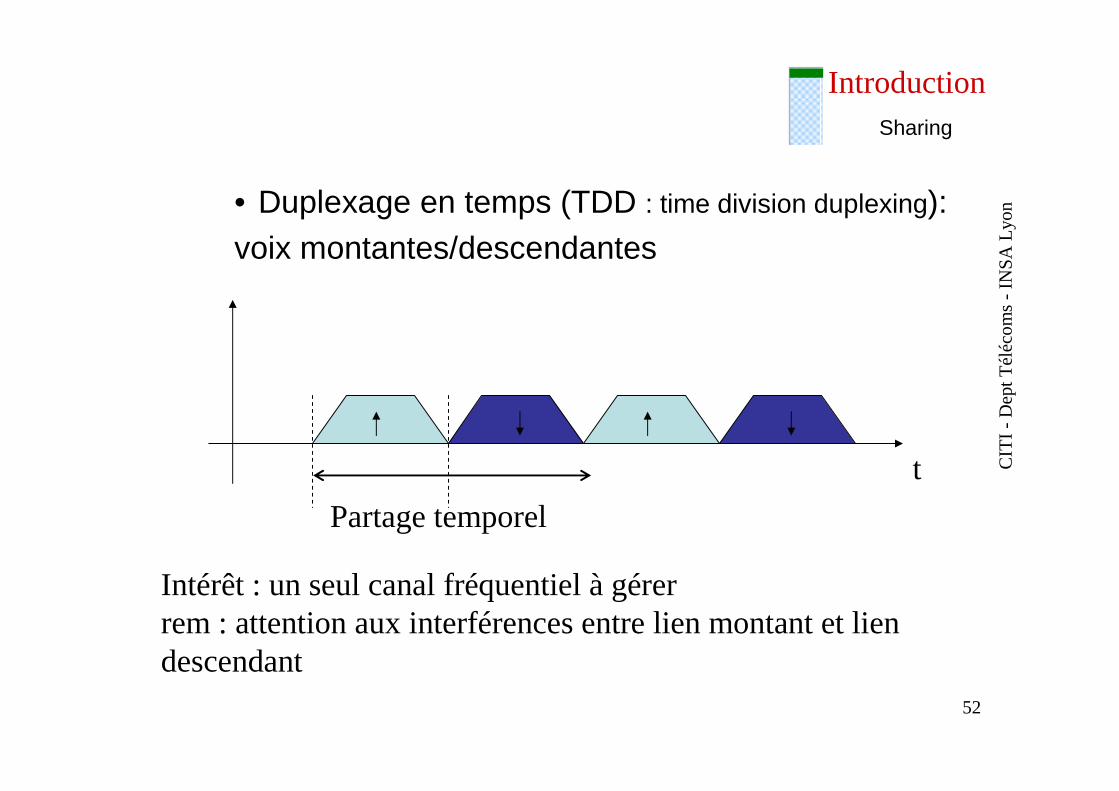
• Duplexage en temps (TDD : time division duplexing): voix montantes/descendantes
t
Partage temporel
Intérêt : un seul canal fréquentiel à gérerrem : attention aux interférences entre lien montant et lien descendant
Sharing
CIT
I -D
ept T
éléc
om
s -
INS
A L
yon
53
Introduction
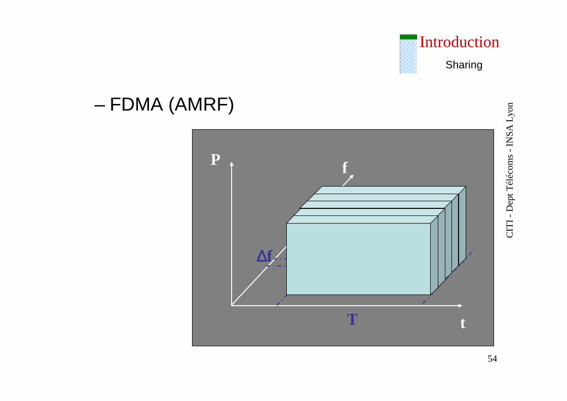
C) Méthodes d ’accès multiples• 1 bande globale : W ; C=Rs x Nb ; Nb=f(SNR)
– théorique C=2xW (2porteuses, 1 bit/porteuse) – pratique : W=1,6Rs; C=2/1,6 x W=1,25xW.
» BER~10-4 =>Eb/No=8dB; SNR=9dB.
• On veut partager ce débit global :– choix parmi : FDMA, TDMA, FTDMA (GSM) ou CDMA
(IS-95, UMTS).
• Critères : – Maximiser l’utilisation des ressources (bits/s/hertz)– Gérer le niveau d’interférences
Sharing
CIT
I -D
ept T
éléc
om
s -
INS
A L
yon
54
Introduction
– FDMA (AMRF)
t
fP
∆∆∆∆f
T
Sharing
CIT
I -D
ept T
éléc
om
s -
INS
A L
yon
55
Introduction
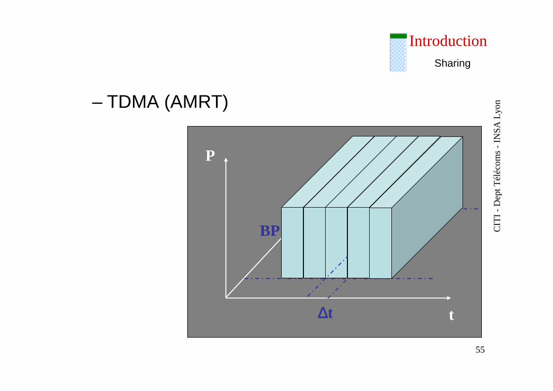
– TDMA (AMRT)
t
fP
BP
∆∆∆∆t
Sharing
CIT
I -D
ept T
éléc
om
s -
INS
A L
yon
56
Introduction
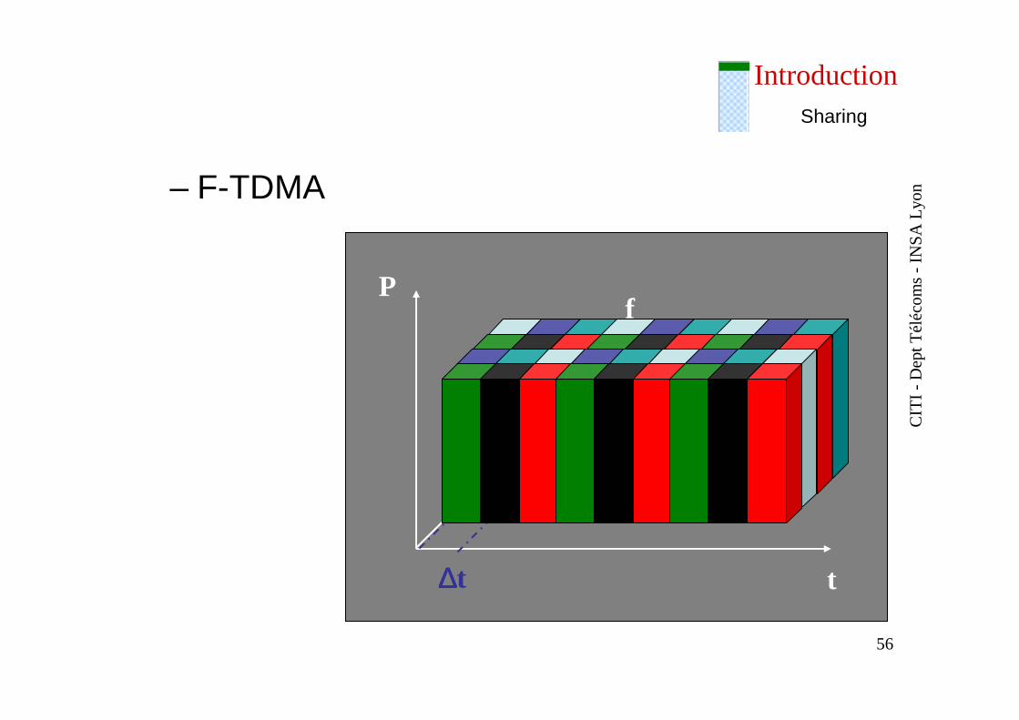
– F-TDMA
t
fP
∆∆∆∆f
∆∆∆∆t
Sharing
CIT
I -D
ept T
éléc
om
s -
INS
A L
yon
57
Introduction
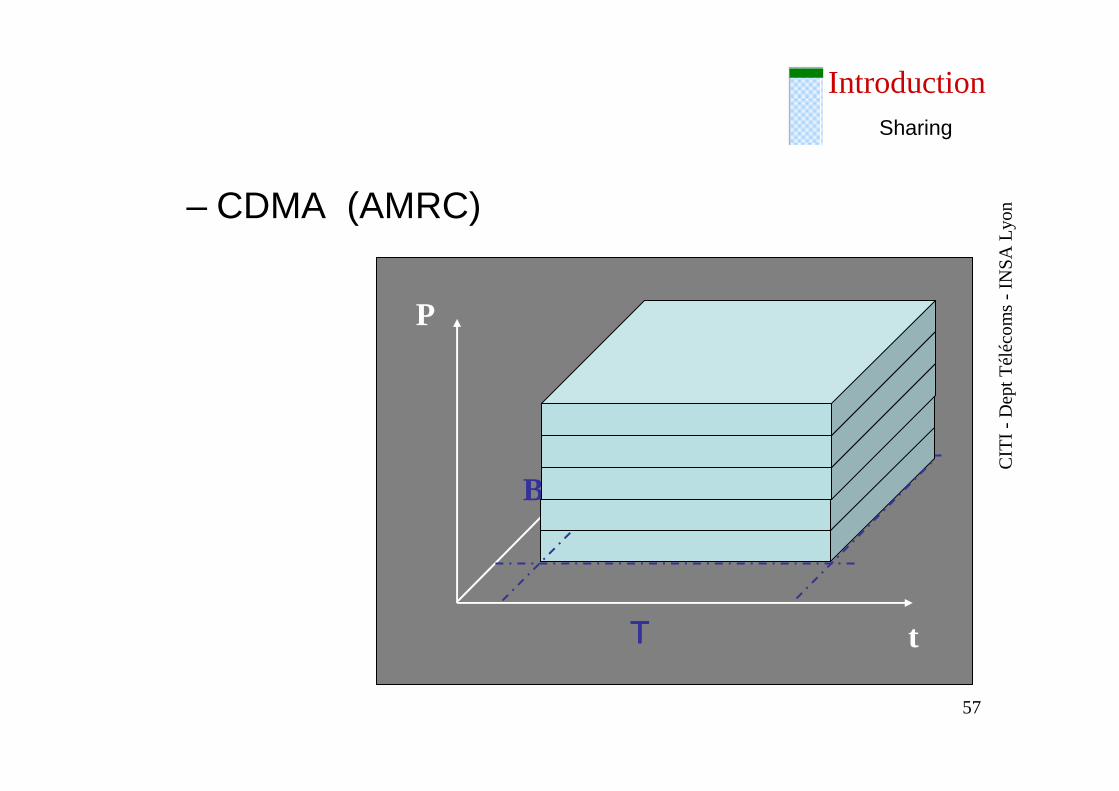
– CDMA (AMRC)
t
fP
BP
ΤΤΤΤ
Sharing
CIT
I -D
ept T
éléc
om
s -
INS
A L
yon
58
IntroductionD) Cas particulier : CSMA/CA
AP
Sharing
CIT
I -D
ept T
éléc
om
s -
INS
A L
yon
59
Introduction
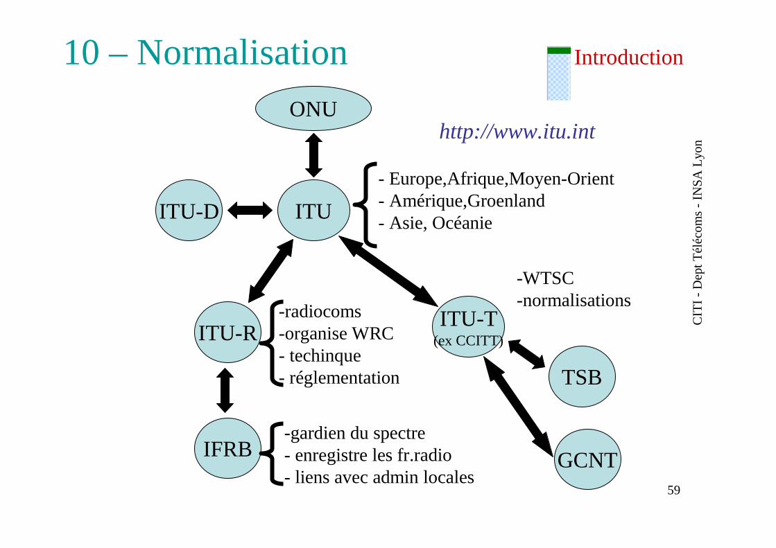
ONU
ITU
ITU-T(ex CCITT)
ITU-D
ITU-R
- Europe,Afrique,Moyen-Orient- Amérique,Groenland- Asie, Océanie
-radiocoms-organise WRC- techinque- réglementation
IFRB-gardien du spectre- enregistre les fr.radio- liens avec admin locales
-WTSC-normalisations
TSB
GCNT
http://www.itu.int
10 – Normalisation
CIT
I -D
ept T
éléc
om
s -
INS
A L
yon
60
Introduction
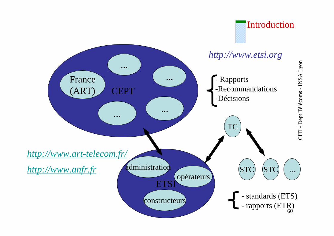
CEPTFrance(ART)
... ...
......
ETSI
- Rapports-Recommandations-Décisions
opérateurs
constructeurs
administration
TC
STC STC ...
- standards (ETS)- rapports (ETR)
http://www.etsi.org
http://www.anfr.fr
http://www.art-telecom.fr/
CIT
I -D
ept T
éléc
om
s -
INS
A L
yon
61
Résumé de l’introduction (à savoir ☺ )
– Les bandes de fréquences (f, λ)
– La modélisation en blocs (pour se repérer dans le cours)
– Les grands principes/théorèmes de propagation
– Modulation/capacité : qu’est-ce qui limite les systèmes?
– Les familles de systèmes radio
– Les types d’interférences
– Les méthodes de partage de ressources
– Qui régule l’utilisation des fréquences