Commodity Connectedness

Francis X. Diebold

University of Pennsylvania

Laura Liu

University of Pennsylvania

Kamil Yılmaz

Koc University

June 27, 2017

Abstract: We use variance decompositions from high-dimensional vector autoregressions to characterizeconnectedness in 19 key commodity return volatilities, 2011-2016. We study both static (full-sample) anddynamic (rolling-sample) connectedness. We summarize and visualize the results using tools from networkanalysis. The results reveal clear clustering of commodities into groups that match traditional industrygroupings, but with some notable differences. The energy sector is most important in terms of sendingshocks to others, and energy, industrial metals, and precious metals are themselves tightly connected.

Key Words: network centrality, network visualization, pairwise connectedness, total directional connect-edness, total connectedness, vector autoregression, variance decomposition, LASSO

JEL codes: G1, C3

Contact Author: F.X. Diebold, fdiebold@sas.upenn.edu

Acknowledgments: For helpful comments we thank an anonymous referee, as well as Gary Gorton, AlainKabundi, Danilo Leiva, Fabrizio Perri, and Xiao Qiao. The usual disclaimer applies.

Contents

1 Introduction 1

2 Commodities Data and Volatility 2

2.1 Price Indices . . . . . . . . . . . . . . . . . . . . . . . . . . . . . . . . . . . . . . . . . . . . . 2

2.2 Realized Volatility . . . . . . . . . . . . . . . . . . . . . . . . . . . . . . . . . . . . . . . . . . 3

3 Benchmark Results I: Static (Full-Sample) Connectedness 5

3.1 Measuring Connectedness . . . . . . . . . . . . . . . . . . . . . . . . . . . . . . . . . . . . . . 5

3.2 System-Wide Connectedness . . . . . . . . . . . . . . . . . . . . . . . . . . . . . . . . . . . . . 7

3.3 To-Degrees and From-Degrees . . . . . . . . . . . . . . . . . . . . . . . . . . . . . . . . . . . . 7

3.4 The Network Graph . . . . . . . . . . . . . . . . . . . . . . . . . . . . . . . . . . . . . . . . . 8

3.5 Six-Group Aggregation . . . . . . . . . . . . . . . . . . . . . . . . . . . . . . . . . . . . . . . . 9

4 Benchmark Results II: Dynamic (Rolling-Sample) Connectedness 11

4.1 On the Economics of Commodity Connectedness Dynamics . . . . . . . . . . . . . . . . . . . 11

4.2 System-Wide Connectedness . . . . . . . . . . . . . . . . . . . . . . . . . . . . . . . . . . . . . 13

4.3 Total Directional Connectedness . . . . . . . . . . . . . . . . . . . . . . . . . . . . . . . . . . 15

5 Conclusion 19

Appendices 19

A Verification of Key Properties of Realized Volatility 19

B Different Horizons (Various h, Fixed p = 3) 20

C Different Dynamics (Fixed h = 10, Various p) 20

1 Introduction

Commodities and commodity markets play a central role in the global economy.1 Hence

commodity market developments are widely chronicled and followed.2 Commodities are a

key input to all countries’ production, and a key output of many emerging economies, so fluc-

tuations in commodity prices may contribute strongly to common business cycle fluctuations

in emerging economies and beyond, as emphasized by Fernandez et al. (2015). Commodities

have also emerged as important financial asset classes (e.g., energy, agriculture, metals), with

properties different from those of “traditional” asset classes like stocks, bonds, and foreign

exchange, as emphasized by Kat and Oomen (2007a) and Kat and Oomen (2007b).

Understanding connectedness, which is central to risk measurement and management,

seems particularly important in the commodities context, particularly for emerging economies

relying heavily on commodities production. Relevant aspects include connectedness across

firms, markets, and countries, both nominal/financial and real. In particular, we have in

mind things like connectedness of commodity company stocks (both within and across coun-

tries), connectedness of commodity prices, and links between commodity price connectedness

and country real output connectedness.

Moreover, connectedness measurement in real time is of special relevance for policy.

Successful real-time policy (and all policy is real-time) demands real-time monitoring, often

exploiting high-frequency data.3 As we shall later describe in detail, the daily commodity

volatilities that we study in this paper are in precisely that tradition, built from key parts

of trade-by-trade intra-day price paths.

Several approaches to connectedness measurement have been considered recently.4 Billio

et al. (2012) use pairwise Granger causality. Bonaldi et al. (2013) work with vector autore-

gressions (VAR’s), which allow for full multivariate dynamic cross-variable interaction and

hence richer connectedness assessment, focusing on connectedness due to cross-lag interac-

tions as opposed to innovation correlations. Diebold and Yilmaz (2009), Diebold and Yilmaz

(2012), and Diebold and Yilmaz (2014) also use VAR’s, but they use variance decomposi-

tions, which account for innovation correlations in addition to dynamic cross-variable inter-

actions.5 Demirer et al. (2016) extend the Diebold-Yilmaz framework to high-dimensional

1For a broad overview from an empirical perspective, see Chevallier and Ielpo (2013).2See, for example, the World Bank Commodity Market Outlook, http://www.worldbank.org/en/

research/commodity-markets.3See, for example, John Taylor’s inaugural Feldstein Lecture at the National Bureau of Economic Re-

search, (http://www.nber.org/feldstein_lecture/feldsteinlecture_2009.html).4For an interpretive survey see Kara et al. (2015).5The Diebold and Yilmaz (2014) framework extends earlier variance-decomposition work by Diebold and

environments, which are increasingly relevant, by incorporating LASSO estimation.

In this paper, we characterize global commodity market connectedness using the Demirer

et al. (2016) framework. This is of interest in a variety of contexts. One such key context

is private-sector investment management strategies, whose portfolio concentration risk is di-

rectly related to connectedness. Another is public-sector monitoring and policy formulation,

because connectedness tends to increase during commodity-market crises, which may then

spill over into the broader macroeconomy.

We proceed as follows. In section 2 we discuss our commodity price indices, our con-

struction and verification of realized return volatility, and our framework for measuring

commodity volatility connectedness. In section 3 we provide benchmark results for static

connectedness, and in section 4 we provide results for dynamic connectedness. We conclude

in section 5, and we explore variations and extensions in several appendices.

2 Commodities Data and Volatility

In this section we describe our commodities data – prices, returns, and range-based return

volatilities – and their properties.

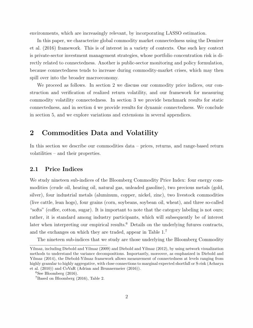
2.1 Price Indices

We study nineteen sub-indices of the Bloomberg Commodity Price Index: four energy com-

modities (crude oil, heating oil, natural gas, unleaded gasoline), two precious metals (gold,

silver), four industrial metals (aluminum, copper, nickel, zinc), two livestock commodities

(live cattle, lean hogs), four grains (corn, soybeans, soybean oil, wheat), and three so-called

“softs” (coffee, cotton, sugar). It is important to note that the category labeling is not ours;

rather, it is standard among industry participants, which will subsequently be of interest

later when interpreting our empirical results.6 Details on the underlying futures contracts,

and the exchanges on which they are traded, appear in Table 1.7

The nineteen sub-indices that we study are those underlying the Bloomberg Commodity

Yilmaz, including Diebold and Yilmaz (2009) and Diebold and Yilmaz (2012), by using network visualizationmethods to understand the variance decompositions. Importantly, moreover, as emphasized in Diebold andYilmaz (2014), the Diebold-Yilmaz framework allows measurement of connectedness at levels ranging fromhighly granular to highly aggregative, with close connections to marginal expected shortfall or S-risk (Acharyaet al. (2010)) and CoVaR (Adrian and Brunnermeier (2016)).

6See Bloomberg (2016).7Based on Bloomberg (2016), Table 2.

2

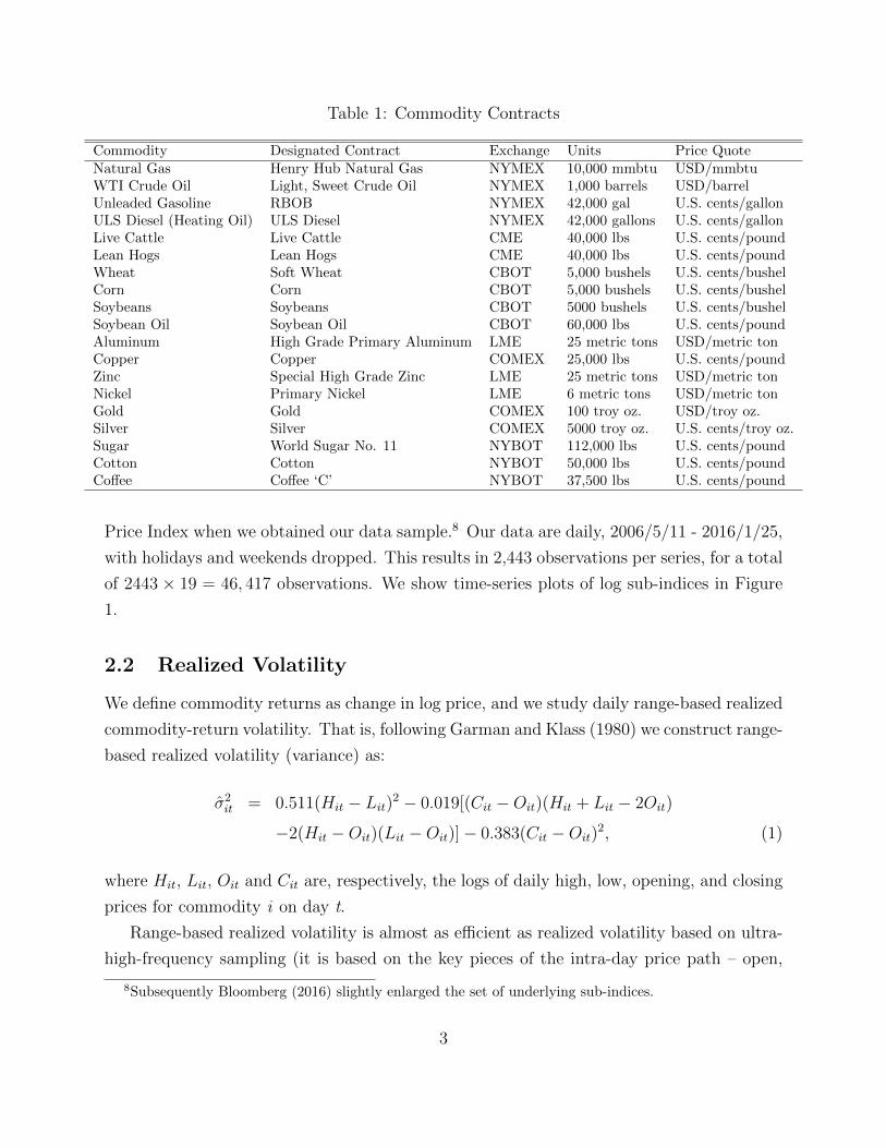
Table 1: Commodity Contracts

Commodity Designated Contract Exchange Units Price QuoteNatural Gas Henry Hub Natural Gas NYMEX 10,000 mmbtu USD/mmbtuWTI Crude Oil Light, Sweet Crude Oil NYMEX 1,000 barrels USD/barrelUnleaded Gasoline RBOB NYMEX 42,000 gal U.S. cents/gallonULS Diesel (Heating Oil) ULS Diesel NYMEX 42,000 gallons U.S. cents/gallonLive Cattle Live Cattle CME 40,000 lbs U.S. cents/poundLean Hogs Lean Hogs CME 40,000 lbs U.S. cents/poundWheat Soft Wheat CBOT 5,000 bushels U.S. cents/bushelCorn Corn CBOT 5,000 bushels U.S. cents/bushelSoybeans Soybeans CBOT 5000 bushels U.S. cents/bushelSoybean Oil Soybean Oil CBOT 60,000 lbs U.S. cents/poundAluminum High Grade Primary Aluminum LME 25 metric tons USD/metric tonCopper Copper COMEX 25,000 lbs U.S. cents/poundZinc Special High Grade Zinc LME 25 metric tons USD/metric tonNickel Primary Nickel LME 6 metric tons USD/metric tonGold Gold COMEX 100 troy oz. USD/troy oz.Silver Silver COMEX 5000 troy oz. U.S. cents/troy oz.Sugar World Sugar No. 11 NYBOT 112,000 lbs U.S. cents/poundCotton Cotton NYBOT 50,000 lbs U.S. cents/poundCoffee Coffee ‘C’ NYBOT 37,500 lbs U.S. cents/pound

Price Index when we obtained our data sample.8 Our data are daily, 2006/5/11 - 2016/1/25,

with holidays and weekends dropped. This results in 2,443 observations per series, for a total

of 2443 × 19 = 46, 417 observations. We show time-series plots of log sub-indices in Figure

1.

2.2 Realized Volatility

We define commodity returns as change in log price, and we study daily range-based realized

commodity-return volatility. That is, following Garman and Klass (1980) we construct range-

based realized volatility (variance) as:

σ2it = 0.511(Hit − Lit)

2 − 0.019[(Cit −Oit)(Hit + Lit − 2Oit)

−2(Hit −Oit)(Lit −Oit)]− 0.383(Cit −Oit)2, (1)

where Hit, Lit, Oit and Cit are, respectively, the logs of daily high, low, opening, and closing

prices for commodity i on day t.

Range-based realized volatility is almost as efficient as realized volatility based on ultra-

high-frequency sampling (it is based on the key pieces of the intra-day price path – open,

8Subsequently Bloomberg (2016) slightly enlarged the set of underlying sub-indices.

3

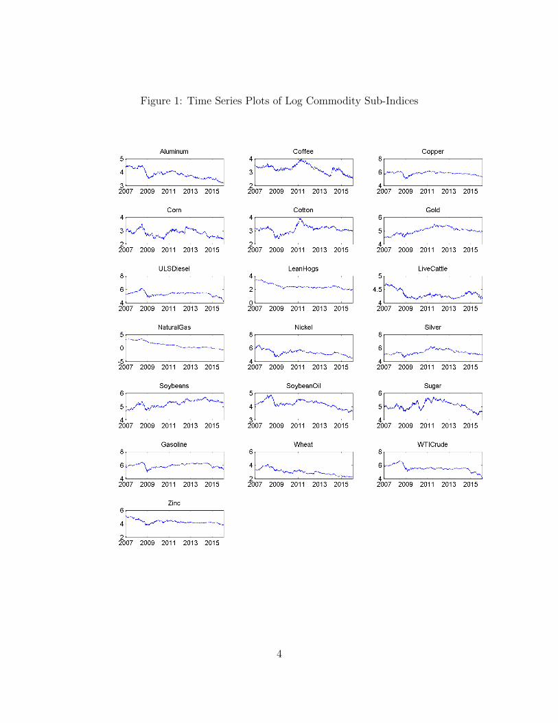
Figure 1: Time Series Plots of Log Commodity Sub-Indices

4

close, high, low), much less tedious to construct, robust to microstructure noise, and widely

available, often for many decades.9

In Appendix A we verify the key properties of realized volatility. Results for other markets

like equities (Andersen et al. (2001a)) and foreign exchange (Andersen et al. (2001b)) indicate

that daily realized volatilities are (1) generally distributed asymmetrically, with a right skew,

(2) approximately Gaussian after taking natural logarithms, and (3) very strongly serially

correlated. Despite the fact that the economics of commodity markets are quite different

from those of foreign exchange or equities, the results in Appendix A make clear that all

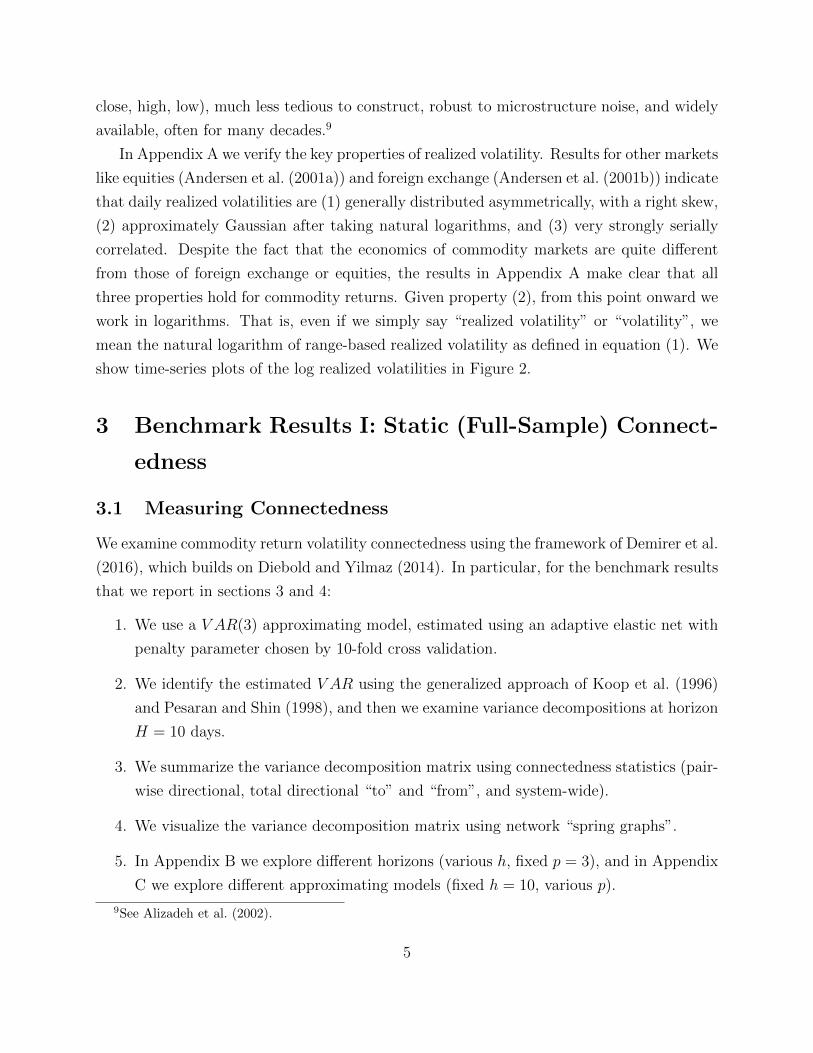
three properties hold for commodity returns. Given property (2), from this point onward we

work in logarithms. That is, even if we simply say “realized volatility” or “volatility”, we

mean the natural logarithm of range-based realized volatility as defined in equation (1). We

show time-series plots of the log realized volatilities in Figure 2.

3 Benchmark Results I: Static (Full-Sample) Connect-

edness

3.1 Measuring Connectedness

We examine commodity return volatility connectedness using the framework of Demirer et al.

(2016), which builds on Diebold and Yilmaz (2014). In particular, for the benchmark results

that we report in sections 3 and 4:

1. We use a V AR(3) approximating model, estimated using an adaptive elastic net with

penalty parameter chosen by 10-fold cross validation.

2. We identify the estimated V AR using the generalized approach of Koop et al. (1996)

and Pesaran and Shin (1998), and then we examine variance decompositions at horizon

H = 10 days.

3. We summarize the variance decomposition matrix using connectedness statistics (pair-

wise directional, total directional “to” and “from”, and system-wide).

4. We visualize the variance decomposition matrix using network “spring graphs”.

5. In Appendix B we explore different horizons (various h, fixed p = 3), and in Appendix

C we explore different approximating models (fixed h = 10, various p).

9See Alizadeh et al. (2002).

5

Figure 2: Time Series Plots of Log Realized Volatilities

6

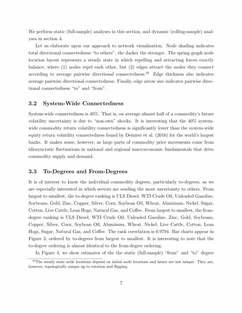
We perform static (full-sample) analyses in this section, and dynamic (rolling-sample) anal-

yses in section 4.

Let us elaborate upon our approach to network visualization. Node shading indicates

total directional connectedness “to others”; the darker the stronger. The spring graph node

location layout represents a steady state in which repelling and attracting forces exactly

balance, where (1) nodes repel each other, but (2) edges attract the nodes they connect

according to average pairwise directional connectedness.10 Edge thickness also indicates

average pairwise directional connectedness. Finally, edge arrow size indicates pairwise direc-

tional connectedness “to” and “from”.

3.2 System-Wide Connectedness

System-wide connectedness is 40%. That is, on average almost half of a commodity’s future

volatility uncertainty is due to “non-own” shocks. It is interesting that the 40% system-

wide commodity return volatility connectedness is significantly lower than the system-wide

equity return volatility connectedness found by Demirer et al. (2016) for the world’s largest

banks. It makes sense, however, as large parts of commodity price movements come from

idiosyncratic fluctuations in national and regional macroeconomic fundamentals that drive

commodity supply and demand.

3.3 To-Degrees and From-Degrees

It is of interest to know the individual commodity degrees, particularly to-degrees, as we

are especially interested in which sectors are sending the most uncertainty to others. From

largest to smallest, the to-degree ranking is ULS Diesel, WTI Crude Oil, Unleaded Gasoline,

Soybeans, Gold, Zinc, Copper, Silver, Corn, Soybean Oil, Wheat, Aluminum, Nickel, Sugar,

Cotton, Live Cattle, Lean Hogs, Natural Gas, and Coffee. From largest to smallest, the from-

degree ranking is ULS Diesel, WTI Crude Oil, Unleaded Gasoline, Zinc, Gold, Soybeans,

Copper, Silver, Corn, Soybean Oil, Aluminum, Wheat, Nickel, Live Cattle, Cotton, Lean

Hogs, Sugar, Natural Gas, and Coffee. The rank correlation is 0.9794. Bar charts appear in

Figure 3, ordered by to-degrees from largest to smallest. It is interesting to note that the

to-degree ordering is almost identical to the from-degree ordering.

In Figure 4, we show estimates of the the static (full-sample) “from” and “to” degree

10The steady state node locations depend on initial node locations and hence are not unique. They are,however, topologically unique up to rotation and flipping.

7

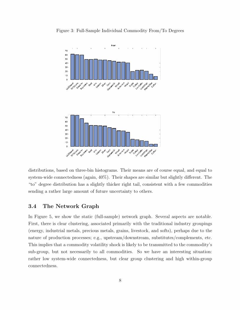
Figure 3: Full-Sample Individual Commodity From/To Degrees

distributions, based on three-bin histograms. Their means are of course equal, and equal to

system-wide connectedness (again, 40%). Their shapes are similar but slightly different. The

“to” degree distribution has a slightly thicker right tail, consistent with a few commodities

sending a rather large amount of future uncertainty to others.

3.4 The Network Graph

In Figure 5, we show the static (full-sample) network graph. Several aspects are notable.

First, there is clear clustering, associated primarily with the traditional industry groupings

(energy, industrial metals, precious metals, grains, livestock, and softs), perhaps due to the

nature of production processes; e.g., upstream/downstream, substitutes/complements, etc.

This implies that a commodity volatility shock is likely to be transmitted to the commodity’s

sub-group, but not necessarily to all commodities. So we have an interesting situation:

rather low system-wide connectedness, but clear group clustering and high within-group

connectedness.

8

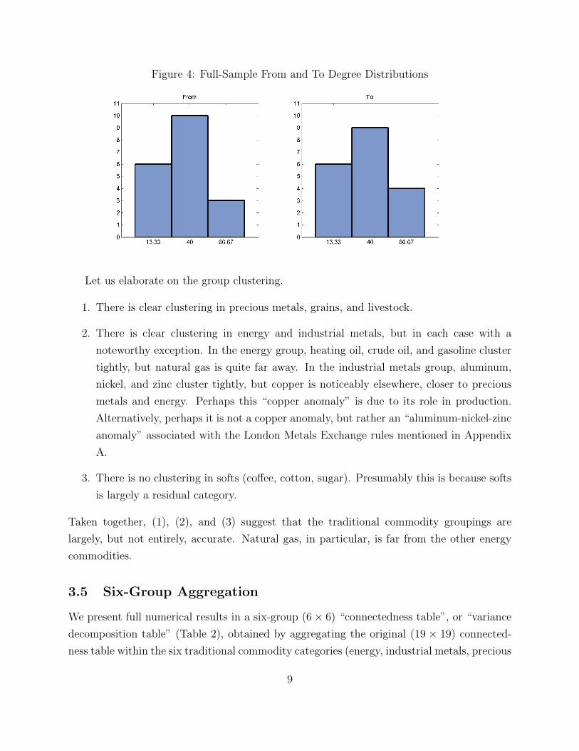
Figure 4: Full-Sample From and To Degree Distributions

Let us elaborate on the group clustering.

1. There is clear clustering in precious metals, grains, and livestock.

2. There is clear clustering in energy and industrial metals, but in each case with a

noteworthy exception. In the energy group, heating oil, crude oil, and gasoline cluster

tightly, but natural gas is quite far away. In the industrial metals group, aluminum,

nickel, and zinc cluster tightly, but copper is noticeably elsewhere, closer to precious

metals and energy. Perhaps this “copper anomaly” is due to its role in production.

Alternatively, perhaps it is not a copper anomaly, but rather an “aluminum-nickel-zinc

anomaly” associated with the London Metals Exchange rules mentioned in Appendix

A.

3. There is no clustering in softs (coffee, cotton, sugar). Presumably this is because softs

is largely a residual category.

Taken together, (1), (2), and (3) suggest that the traditional commodity groupings are

largely, but not entirely, accurate. Natural gas, in particular, is far from the other energy

commodities.

3.5 Six-Group Aggregation

We present full numerical results in a six-group (6× 6) “connectedness table”, or “variance

decomposition table” (Table 2), obtained by aggregating the original (19 × 19) connected-

ness table within the six traditional commodity categories (energy, industrial metals, precious

9

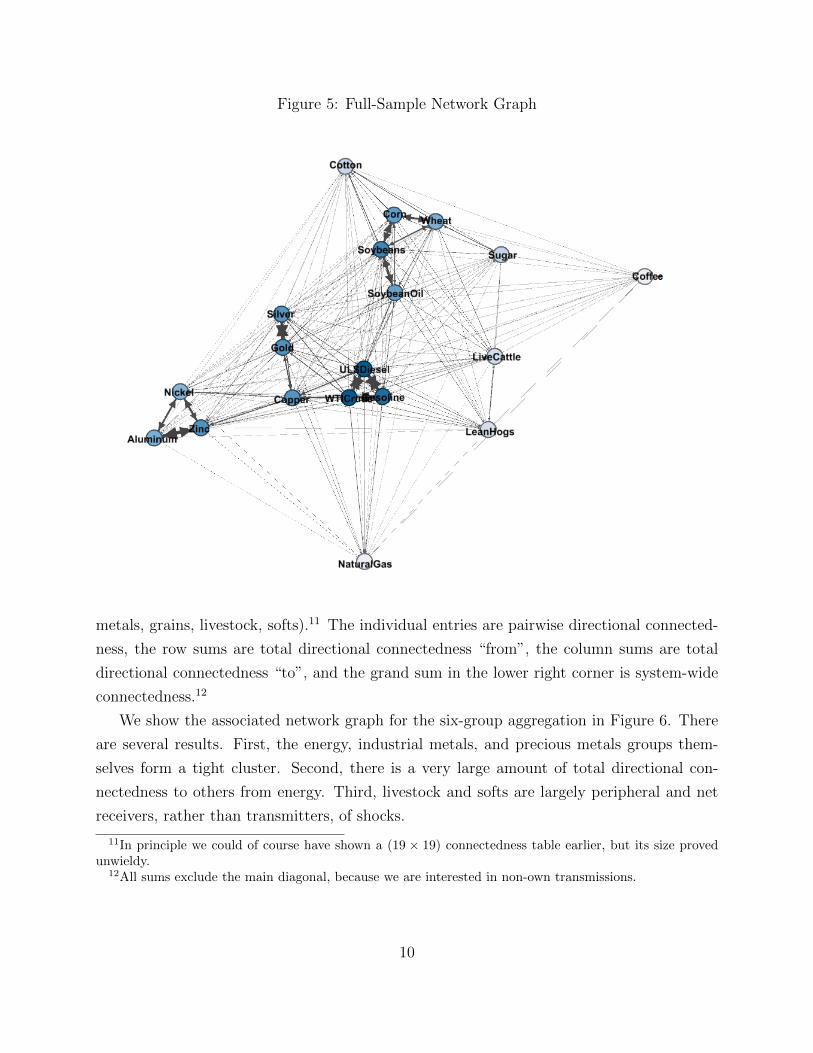
Figure 5: Full-Sample Network Graph

metals, grains, livestock, softs).11 The individual entries are pairwise directional connected-

ness, the row sums are total directional connectedness “from”, the column sums are total

directional connectedness “to”, and the grand sum in the lower right corner is system-wide

connectedness.12

We show the associated network graph for the six-group aggregation in Figure 6. There

are several results. First, the energy, industrial metals, and precious metals groups them-

selves form a tight cluster. Second, there is a very large amount of total directional con-

nectedness to others from energy. Third, livestock and softs are largely peripheral and net

receivers, rather than transmitters, of shocks.

11In principle we could of course have shown a (19 × 19) connectedness table earlier, but its size provedunwieldy.

12All sums exclude the main diagonal, because we are interested in non-own transmissions.

10

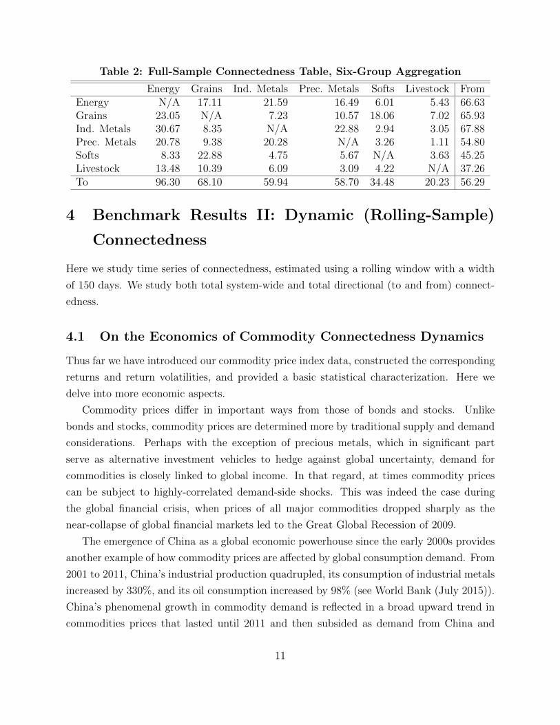
Table 2: Full-Sample Connectedness Table, Six-Group Aggregation

Energy Grains Ind. Metals Prec. Metals Softs Livestock FromEnergy N/A 17.11 21.59 16.49 6.01 5.43 66.63Grains 23.05 N/A 7.23 10.57 18.06 7.02 65.93Ind. Metals 30.67 8.35 N/A 22.88 2.94 3.05 67.88Prec. Metals 20.78 9.38 20.28 N/A 3.26 1.11 54.80Softs 8.33 22.88 4.75 5.67 N/A 3.63 45.25Livestock 13.48 10.39 6.09 3.09 4.22 N/A 37.26To 96.30 68.10 59.94 58.70 34.48 20.23 56.29

4 Benchmark Results II: Dynamic (Rolling-Sample)

Connectedness

Here we study time series of connectedness, estimated using a rolling window with a width

of 150 days. We study both total system-wide and total directional (to and from) connect-

edness.

4.1 On the Economics of Commodity Connectedness Dynamics

Thus far we have introduced our commodity price index data, constructed the corresponding

returns and return volatilities, and provided a basic statistical characterization. Here we

delve into more economic aspects.

Commodity prices differ in important ways from those of bonds and stocks. Unlike

bonds and stocks, commodity prices are determined more by traditional supply and demand

considerations. Perhaps with the exception of precious metals, which in significant part

serve as alternative investment vehicles to hedge against global uncertainty, demand for

commodities is closely linked to global income. In that regard, at times commodity prices

can be subject to highly-correlated demand-side shocks. This was indeed the case during

the global financial crisis, when prices of all major commodities dropped sharply as the

near-collapse of global financial markets led to the Great Global Recession of 2009.

The emergence of China as a global economic powerhouse since the early 2000s provides

another example of how commodity prices are affected by global consumption demand. From

2001 to 2011, China’s industrial production quadrupled, its consumption of industrial metals

increased by 330%, and its oil consumption increased by 98% (see World Bank (July 2015)).

China’s phenomenal growth in commodity demand is reflected in a broad upward trend in

commodities prices that lasted until 2011 and then subsided as demand from China and

11

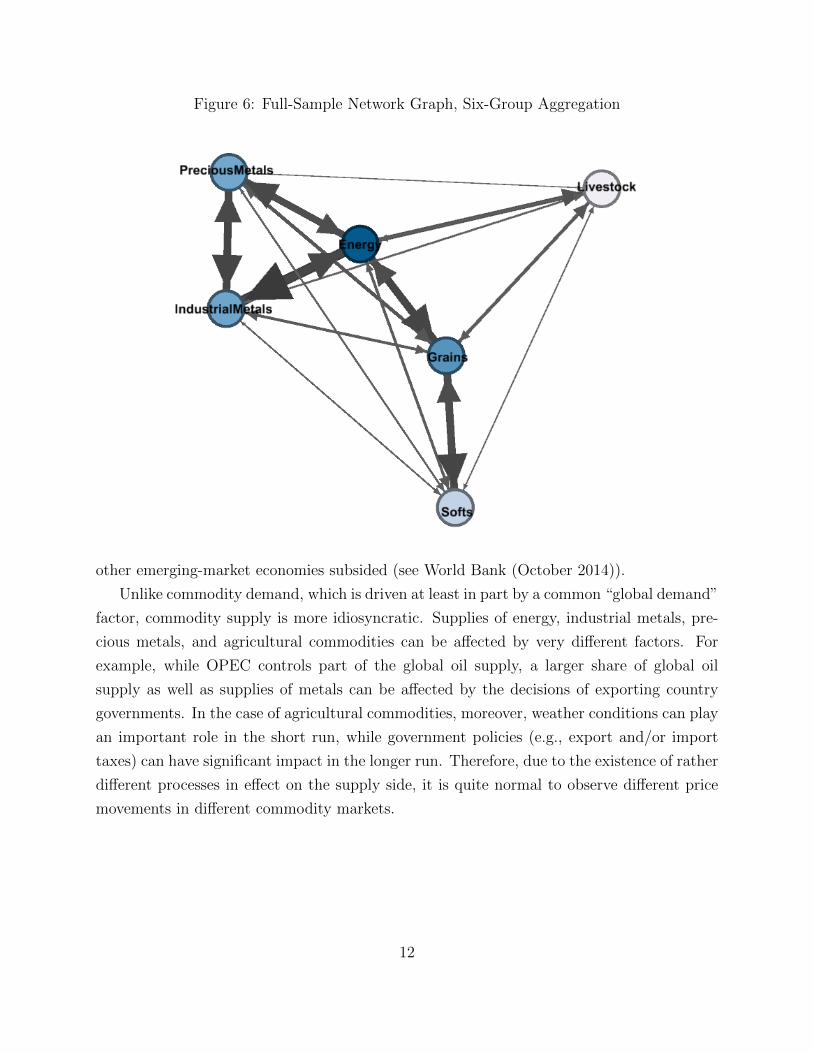
Figure 6: Full-Sample Network Graph, Six-Group Aggregation

other emerging-market economies subsided (see World Bank (October 2014)).

Unlike commodity demand, which is driven at least in part by a common “global demand”

factor, commodity supply is more idiosyncratic. Supplies of energy, industrial metals, pre-

cious metals, and agricultural commodities can be affected by very different factors. For

example, while OPEC controls part of the global oil supply, a larger share of global oil

supply as well as supplies of metals can be affected by the decisions of exporting country

governments. In the case of agricultural commodities, moreover, weather conditions can play

an important role in the short run, while government policies (e.g., export and/or import

taxes) can have significant impact in the longer run. Therefore, due to the existence of rather

different processes in effect on the supply side, it is quite normal to observe different price

movements in different commodity markets.

12

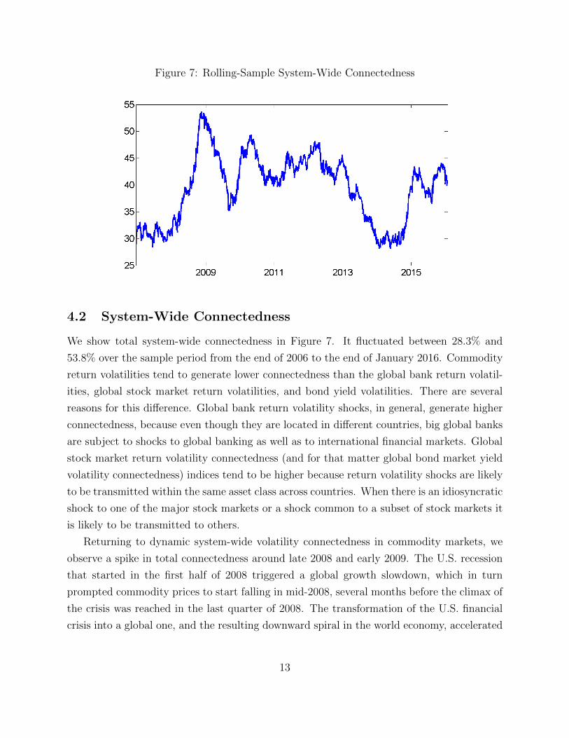
Figure 7: Rolling-Sample System-Wide Connectedness

4.2 System-Wide Connectedness

We show total system-wide connectedness in Figure 7. It fluctuated between 28.3% and

53.8% over the sample period from the end of 2006 to the end of January 2016. Commodity

return volatilities tend to generate lower connectedness than the global bank return volatil-

ities, global stock market return volatilities, and bond yield volatilities. There are several

reasons for this difference. Global bank return volatility shocks, in general, generate higher

connectedness, because even though they are located in different countries, big global banks

are subject to shocks to global banking as well as to international financial markets. Global

stock market return volatility connectedness (and for that matter global bond market yield

volatility connectedness) indices tend to be higher because return volatility shocks are likely

to be transmitted within the same asset class across countries. When there is an idiosyncratic

shock to one of the major stock markets or a shock common to a subset of stock markets it

is likely to be transmitted to others.

Returning to dynamic system-wide volatility connectedness in commodity markets, we

observe a spike in total connectedness around late 2008 and early 2009. The U.S. recession

that started in the first half of 2008 triggered a global growth slowdown, which in turn

prompted commodity prices to start falling in mid-2008, several months before the climax of

the crisis was reached in the last quarter of 2008. The transformation of the U.S. financial

crisis into a global one, and the resulting downward spiral in the world economy, accelerated

13

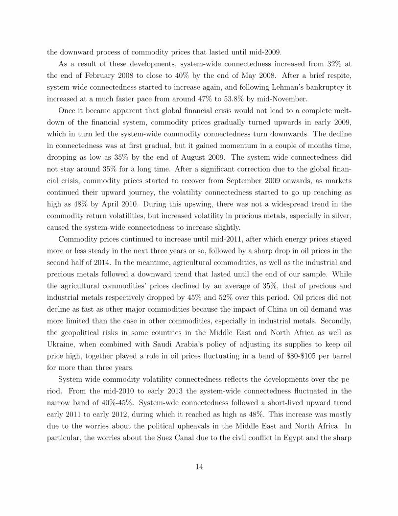
the downward process of commodity prices that lasted until mid-2009.

As a result of these developments, system-wide connectedness increased from 32% at

the end of February 2008 to close to 40% by the end of May 2008. After a brief respite,

system-wide connectedness started to increase again, and following Lehman’s bankruptcy it

increased at a much faster pace from around 47% to 53.8% by mid-November.

Once it became apparent that global financial crisis would not lead to a complete melt-

down of the financial system, commodity prices gradually turned upwards in early 2009,

which in turn led the system-wide commodity connectedness turn downwards. The decline

in connectedness was at first gradual, but it gained momentum in a couple of months time,

dropping as low as 35% by the end of August 2009. The system-wide connectedness did

not stay around 35% for a long time. After a significant correction due to the global finan-

cial crisis, commodity prices started to recover from September 2009 onwards, as markets

continued their upward journey, the volatility connectedness started to go up reaching as

high as 48% by April 2010. During this upswing, there was not a widespread trend in the

commodity return volatilities, but increased volatility in precious metals, especially in silver,

caused the system-wide connectedness to increase slightly.

Commodity prices continued to increase until mid-2011, after which energy prices stayed

more or less steady in the next three years or so, followed by a sharp drop in oil prices in the

second half of 2014. In the meantime, agricultural commodities, as well as the industrial and

precious metals followed a downward trend that lasted until the end of our sample. While

the agricultural commodities’ prices declined by an average of 35%, that of precious and

industrial metals respectively dropped by 45% and 52% over this period. Oil prices did not

decline as fast as other major commodities because the impact of China on oil demand was

more limited than the case in other commodities, especially in industrial metals. Secondly,

the geopolitical risks in some countries in the Middle East and North Africa as well as

Ukraine, when combined with Saudi Arabia’s policy of adjusting its supplies to keep oil

price high, together played a role in oil prices fluctuating in a band of $80-$105 per barrel

for more than three years.

System-wide commodity volatility connectedness reflects the developments over the pe-

riod. From the mid-2010 to early 2013 the system-wide connectedness fluctuated in the

narrow band of 40%-45%. System-wde connectedness followed a short-lived upward trend

early 2011 to early 2012, during which it reached as high as 48%. This increase was mostly

due to the worries about the political upheavals in the Middle East and North Africa. In

particular, the worries about the Suez Canal due to the civil conflict in Egypt and the sharp

14

cut in Libya’s oil production due to the civil war in the country fed into the oil price volatility

which in turn contributed to the system-wide connectedness in commodity markets. After

the overthrow of Qaddafi regime in Libya 2011, the political crisis in Egypt was resolved

with a coup d’etat in mid-July 2013. Following the turn of events in Egypt, volatility in oil

prices subsided and the system-wide connectedness started to decline from around 37% in

mid-July 2013 to 28.5% within six months.

After fluctuating around 30% for several months, system-wide connectedness started to

increase from its lows of 30% in July 2014 to reach 43% by the early 2015. The latest upward

move in system-wide connectedness was due to worries about the civil war in Ukraine and

whether it would lead to the temporary suspension of oil supplies from the Russian Federation

to the world market.

At the same time, military actions of Russian-backed separatists increased confrontation

between Russia, on the one side, and the U.S. and the EU, on the other side. It is speculated

that as the tensions between the two sides increased, Saudi Arabia decided to change its

policy of playing the marginal supplier which aims to keep oil prices high. With this policy

change Saudi Arabia wanted to push high cost shale frackers out of business. Thanks to high

global oil prices shale frackers were able to profitably increase global supply of oil, which

threatened the dominant position of OPEC and in particular, Saudi Arabia, in the long-run.

Secondly, Saudi Arabia helped the U.S. to increase pressure on the Russian government,

which had become increasingly belligerent not only in Ukraine but in other civil unrests in

parts of the world. As a result, the oil price was almost halved from around $100 at the end

of July 2014 to around $50 by the end of the year.

After staying above 40% for several months, system-wide connectedness dropped to 37%

in the summer of 2015, as the oil price ended its downward spiral and settled around $50

per barrel. However, news about China’s financial market troubles in August 2015 increased

tensions and system-wide connectedness not only in commodity markets but in all financial

markets. As a result, system-wide connectedness increased by more than five percentage

points within a month and later reached 44% by the end of October 2015.

4.3 Total Directional Connectedness

In this section we analyze the dynamics of directional connectedness of individual commodi-

ties as well as commodity groups, based on net total directional connectedness graphs (“to”

- “from”) in Figure 8.

As our discussion of the dynamic system-wide connectedness in the previous section

15

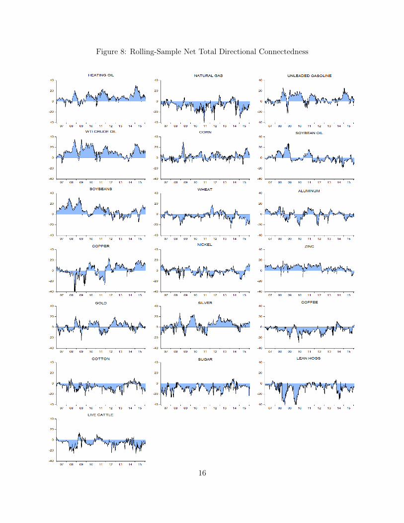
Figure 8: Rolling-Sample Net Total Directional Connectedness

16

showed, and as Figure 8 confirms, oil played quite an important role in the commodity

market connectedness. Its net connectedness is higher than all other commodities for an

overwhelming majority of the rolling sub-sample windows considered. Both in earlier and

later parts of the period, net connectedness of oil reached as high as 30-35% range. The only

sub-periods during which the net connectedness of crude oil was lower are the first half of

2007, and the period from the second half of 2013 to July 2014.

Starting in the first quarter of 2008, the crude oil price skyrocketed from around $60 in

February 2007 to reach $141 per barrel by the first week of July 2008. After that moment,

however, the oil price started to come down as the worries about U.S. economic performance

intensified along with the signs of slowdown in many countries. As the downturn started in

the oil price, oil return volatility increased substantially. Along with the rising oil return

volatility, system-wide volatility connectedness increased from around 40% in early July 2008

to 53% by the end of October 2008. Over the same period net connectedness of WTI crude

oil increased from 10% to 35%, the highest net connectedness level generated by a commodity

for all rolling subsample windows considered (see Figure 8).

By the end of October 2008, the crude oil price dropped to $60 per barrel. However,

the downward spiral in the price of oil continued until the third week of December, with

a minimum price of $31 per barrel. As the oil price lost its downward momentum, its net

connectedness oil dropped to around 10% by the end of 2008. Once the oil price recovers to

reach closer to $60 per barrel, we observe that net volatility connectedness (hence volatility)

of oil returns started to increase significantly and reached to 35% by mid-July 2009.

Heating oil, soybeans and zinc are the three commodities that followed crude oil in

generating very high levels of net connectedness to other commodities over all subsamples

considered. Heating oil is also in the energy commodities group. Its net connectedness to

others follows a trajectory which resembles to that of crude oil.

Soybeans have high net connectedness, not because they are an important consumption

item for households around the world, but rather because they are used in the biofuel pro-

duction. Soybeans’ net connectedness reached as high as 28% in March 2008 and last quarter

of 2008 and first half of 2009. Unlike crude oil, soybeans’ net connectedness increased in

January 2008 (exactly around the FOMC’s emergency conference-call meeting on January

22) and at the end of February and beginning of March 2008. During this period, crude

oil prices were still on an upward move with a net connectedness of only around 10%. A

similar asymmetric move between the net connectedness of crude oil and soybeans occurred

in the first half of 2009. While crude oil’s net connectedness declined from its peak at the

17

end of October 2008 to a low of -6% in the first week of April 2009, during this period the

net connectedness of soybeans increased to reach 28% level.

Zinc is actually the only commodity that generated net positive connectedness to others

throughout the period from 2006 to 2016. Throughout the period, zinc had small but positive

(between 5 to 10%) net connectedness from the beginning of the sample to the end of 2012.

Its net connectedness declined significantly since late 2012 to less than 5%, yet continued to

stay on the positive side.

As for energy commodities, unleaded gasoline is the third in terms of generating net

connectedness to other commodities. Again its net connectedness followed quiet a similar

behavior over time to that of crude oil. The only energy commodity that is a net recipient of

connectedness from others is natural gas. Natural gas is the energy market with the weakest

link to the economic news flow, even when accounting for periods of recession. Reflecting

this fact, its connectedness to others and from others are much lower than those of other

energy commodities. As such its return volatility is likely to be affected by the return

volatilities of other energy commodities. That is why its net connectedness was negative for

an overwhelming majority of rolling sample windows, as shown in Figure 8.

We also need to focus on the net connectedness of copper. While its net connectedness

was negative during the U.S. and global financial crisis in 2007 through 2009 and during the

2011 European debt crisis, copper has generated positive net connectedness since early 2012.

Copper prices declined by more than 50% since the end of 2010, from a high of $9,800 per

ton to a low of $4,700 per ton at the end of 2015. The decline in the price of copper and

its increasing contribution to system-wide connectedness are closely related to the Chinese

slowdown in recent years. Other industrial metals, such as zinc, nickel, and aluminum also

experienced significant price drops over the period, but none of them had net connectedness

as high as copper. We have already covered zinc above. The other two industrial metals,

aluminum and nickel, displayed both positive and negative episodes. When considered all

together industrial metals, industrial metals generated positive net connectedness to other

commodity groups (ranging from 5 to 20%) for almost all rolling window samples.

Among the precious metals, silver has higher net connectedness than gold for most of the

period covered. During the global financial crisis, in the second half of 2009 and first half

of 2010, and since the end of 2011, silver’s net connectedness is much higher (sometimes as

high as 20%) than that of gold (see Figure 8).

Soft commodities (coffee, cotton and sugar) and livestock (lean hogs and live cattle) all

have negative connectedness for almost all rolling sample windows, indicating that their

18

prices on average are influenced by other commodities and/or commodity groups (see Fig-

ure 8).

5 Conclusion

We have estimated and examined the network graph for a set of major commodity sub-

index volatilities. The results reveal clear clustering of commodities into groups that match

traditional industry groupings, but with some notable differences. The energy sector is most

important in terms of sending shocks to others, and energy, industrial metals, and precious

metals are themselves tightly connected.

Appendices

A Verification of Key Properties of Realized Volatility

Results for other markets like equities (Andersen et al. (2001a)) and foreign exchange (An-

dersen et al. (2001b)) indicate that daily realized volatilities are (1) generally distributed

asymmetrically, with a right skew, but approximately Gaussian after taking natural loga-

rithms, and (2) very strongly serially correlated. The economics of commodity markets are

quite different from those of foreign exchange or equities, however, so here we provide an

examination of fundamental distributional and dynamic properties of commodity volatilities.

Let us start with distributional aspects. As obviously revealed in the Gaussian Q-Q plots

of Figure 9, the distribution of realized commodity volatility is strongly skewed right. This is

not surprising, because volatilities are bounded below by zero and experience occasional large

bursts. The real issue is whether log commodity volatilities are approximately Gaussian, as

with foreign exchange and equities. As shown in the Gaussian Q-Q plots for log returns in

Figure 10, the answer is mostly yes.13

Finally, we consider dynamics. In Figure 11 we show volatility autocorrelations. They

decay, which is consistent with covariance stationarity, but they decay very slowly, indicating

highly persistent, if nevertheless mean-reverting, dynamics.

13The only exceptions to approximate log-normality are three industrial metals (aluminum, nickel, zinc),as clearly shown in the Gaussian Q-Q plots of Figure 10. All are traded on the London metals exchange(LME), and they are the only commodities in our data set traded on that exchange.

19

B Different Horizons (Various h, Fixed p = 3)

It is of interest to explore connectedness at different horizons h. On the one hand, one might

hope for results robust to horizon. On the other hand, upon further consideration, it is not

obvious why the results should be robust, or whether such robustness is “desirable”. This

point is related to different notions of network centrality; one can assess 1-step through the

adjacency matrix A, 2-step through A2, and so on to ∞-step (eigenvalue centrality).

First consider static connectedness. In Figure 12, we show static (full-sample) V AR(3)

network connectedness graphs for six variance decomposition horizons: h = 2, 10, 20, ..., 50

days. The different subgraphs are rotated to enhance multiple comparisons. The topology

appears strongly robust to horizon.14

C Different Dynamics (Fixed h = 10, Various p)

We already noted the very high persistence in commodity return volatilities, as is common

across many assets and asset classes. Indeed there may even be long memory, as empha-

sized in Andersen et al. (2003). To allow for that possibility, we also explored a variety of

higher-order approximating models, estimation of which is feasible despite profligate param-

eterizations, given the regularization achieved by the LASSO.

In Figure 13, we show static (full-sample) h = 10 network connectedness graphs for six

V AR lag orders, p = 3, 5, 10, 15, 20, 25. The different subgraphs are rotated to enhance

multiple comparisons. The topology appears strongly robust to lag order.

14The scaling, however, differs across the subgraphs; otherwise the small-h graphs would be tiny and thelarge-h graphs would be huge.

20

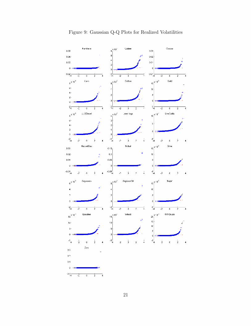
Figure 9: Gaussian Q-Q Plots for Realized Volatilities

21

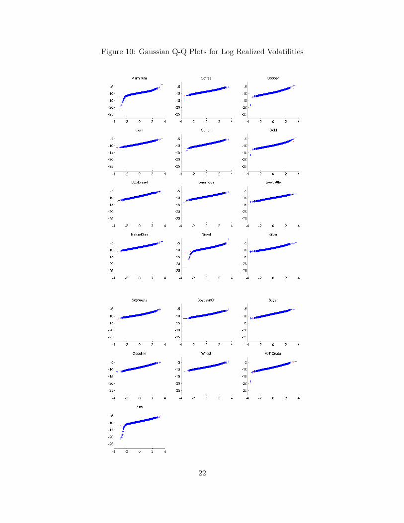
Figure 10: Gaussian Q-Q Plots for Log Realized Volatilities

22

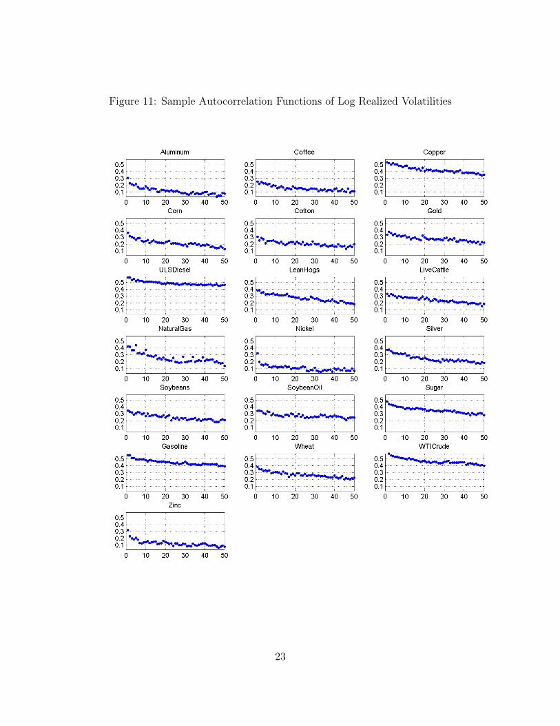
Figure 11: Sample Autocorrelation Functions of Log Realized Volatilities

23

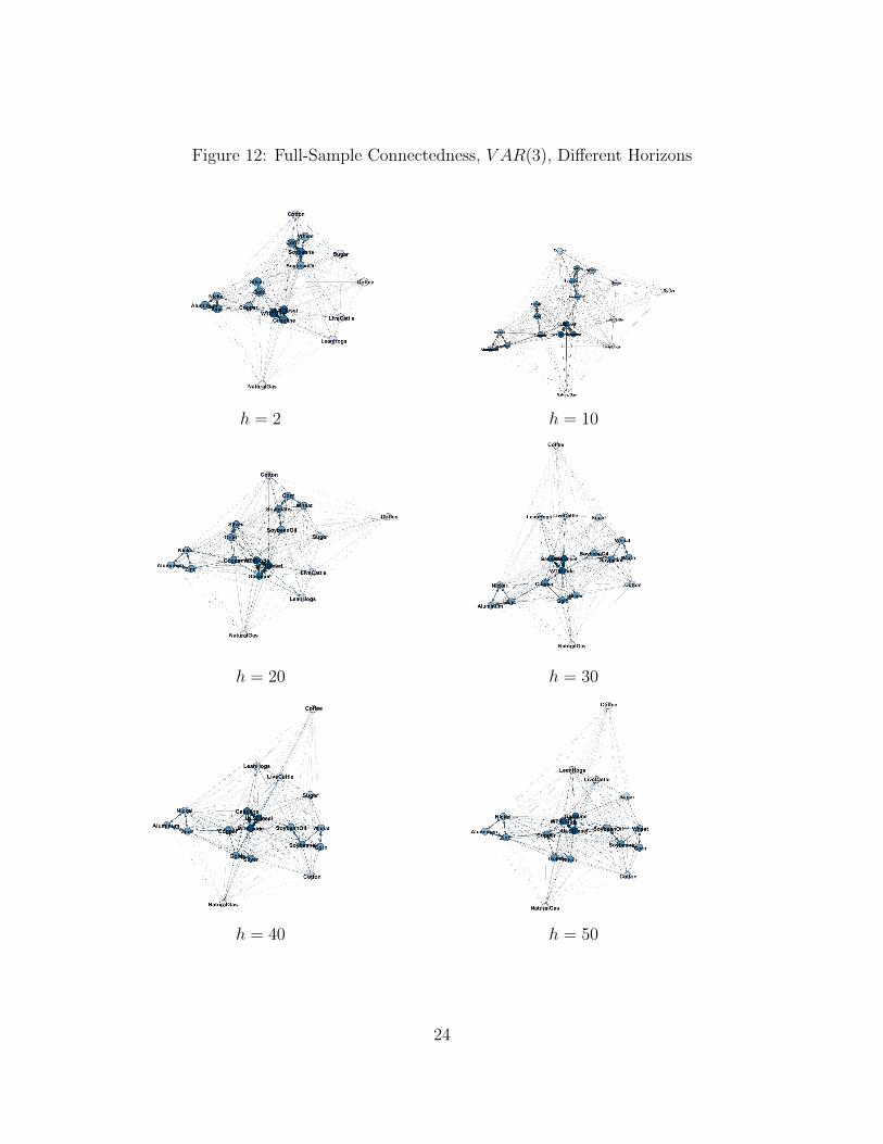
Figure 12: Full-Sample Connectedness, V AR(3), Different Horizons

h = 2 h = 10

h = 20 h = 30

h = 40 h = 50

24

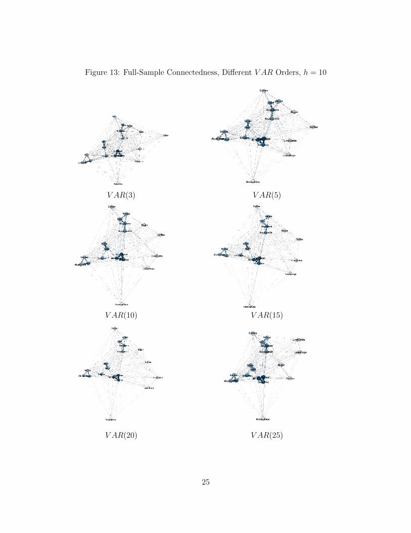
Figure 13: Full-Sample Connectedness, Different V AR Orders, h = 10

V AR(3) V AR(5)

V AR(10) V AR(15)

V AR(20) V AR(25)

25

References

Acharya, V.V., L. Pedersen, T. Philippon, and M. Richardson (2010), “Measuring Systemic

Risk,” Manuscript, New York University.

Adrian, T. and M. Brunnermeier (2016), “CoVaR,” American Economic Review , 106, 1705–

1741.

Alizadeh, S., M.W. Brandt, and F.X. Diebold (2002), “Range-Based Estimation of Stochastic

Volatility Models,” Journal of Finance, 57, 1047–1091.

Andersen, T.G., T. Bollerslev, F.X. Diebold, and H. Ebens (2001a), “The distribution of

realized stock return volatility,” Journal of Financial Economics , 61, 43–76.

Andersen, T.G., T. Bollerslev, F.X. Diebold, and P. Labys (2001b), “The distribution of

realized exchange rate volatility,” Journal of the American Statistical Association, 96,

42–55.

Andersen, T.G., T. Bollerslev, F.X. Diebold, and P. Labys (2003), “Modeling and forecasting

realized volatility,” Econometrica, 71, 579–625.

Billio, M., M. Getmansky, A.W. Lo, and L. Pelizzon (2012), “Econometric Measures of Con-

nectedness and Systemic Risk in the Finance and Insurance Sectors,” Journal of Financial

Economics , 104, 535–559.

Bloomberg (2016), “Index Methodology: The Bloomberg Commodity Index Family,” https:

//www.bbhub.io/indices/sites/2/2016/05/BCOM-Methodology-April-2016.pdf.

Bonaldi, P., A. Hortacsu, and J. Kastl (2013), “An Empirical Analysis of Systemic Risk in

the EURO-zone,” Manuscript, University of Chicago.

Chevallier, J. and F. Ielpo (2013), The Economics of Commodity Markets, John Wiley.

Demirer, M., F.X. Diebold, L. Liu, and K. Yilmaz (2016), “Estimating Global Bank Net-

work Connectedness,” SSRN Working Paper 2631479, available at http://ssrn.com/

abstract=2631479.

Diebold, F.X. and K. Yilmaz (2009), “Measuring Financial Asset Return and Volatility

Spillovers, with Application to Global Equity Markets,” Economic Journal , 119, 158–

171.

26

Diebold, F.X. and K. Yilmaz (2012), “Better to Give than to Receive: Predictive Measure-

ment of Volatility Spillovers (with discussion),” International Journal of Forecasting , 28,

57–66.

Diebold, F.X. and K. Yilmaz (2014), “On the Network Topology of Variance Decompositions:

Measuring the Connectedness of Financial Firms,” Journal of Econometrics , 182, 119–

134.

Fernandez, A., A. Gonzalez, and D. Rodriguez (2015), “Sharing a Ride on the Com-

modities Roller Coaster: Common Factors in Business Cycles of Emerging Economies,”

Inter-American Development Bank Working Paper Series No. IDB-WP-640, available

at http://www.iadb.org/en/research-and-data/publication-details,3169.html?

pub_id=IDB-WP-640.

Garman, M. B. and M. J. Klass (1980), “On the Estimation of Security Price Volatilities

From Historical Data,” Journal of Business , 53, 67–78.

Kara, G.I., M.H. Tian, and M. Yellen (2015), “Taxonomy of Studies on Interconnectedness,”

SSRN Working Paper 2704072, available at http://ssrn.com/abstract=2704072.

Kat, H.M. and R.C.A Oomen (2007a), “What Every Investor Should Know About Com-

modities, Part I,” Journal of Investment Management , 5:1, 4-28.

Kat, H.M. and R.C.A Oomen (2007b), “What Every Investor Should Know About Com-

modities, Part II: Multivariate Return Analysis,” Journal of Investment Management , 5:3,

16-40.

Koop, G., M.H. Pesaran, and S.M. Potter (1996), “Impulse Response Analysis in Nonlinear

Multivariate Models,” Journal of Econometrics , 74, 119–147.

Pesaran, H.H. and Y. Shin (1998), “Generalized Impulse Response Analysis in Linear Mul-

tivariate Models,” Economics Letters , 58, 17–29.

World Bank (July 2015), Commodity Market Outlook .

World Bank (October 2014), Commodity Market Outlook .

27