Combinatorial functional and differential equations ... · Combinatorial functional and differential equations applied to differential posets Matías Menni Conicet – Liﬁa, Universidad

Discrete Mathematics 308 (2008) 1864–1888www.elsevier.com/locate/disc

Combinatorial functional and differential equations applied todifferential posets�

Matías MenniConicet – Lifia, Universidad Nacional de La Plata, 50 y 115 s/n (1900) La Plata, Argentina

Received 13 July 2006; received in revised form 10 April 2007; accepted 18 April 2007Available online 6 May 2007

Abstract

We give combinatorial proofs of the primary results developed by Stanley for deriving enumerative properties of differentialposets. In order to do this we extend the theory of combinatorial differential equations developed by Leroux and Viennot.© 2007 Elsevier B.V. All rights reserved.

Keywords: Differential posets; Y-graphs; Joyal species; Combinatorial differential equations

1. Introduction

The class of posets known as Y-graphs or differential posets was discovered independently by Fomin [4,6] and byStanley [18]. Intuitively, the definition of this class of graphs captures the essential structural properties of Young’slattice (i.e. partitions ordered by inclusion of Young diagrams) which allow a correspondence between Hasse walks inthe poset and certain permutations.

Although both authors seem to have been motivated by similar enumerative applications, their strategies are quitedifferent. Fomin shows that forY-graphs it is possible to define variants of the Schensted algorithm which realize explicitbijections between walks and permutations. On the other hand: “In [18] Stanley was able to derive many enumerativeresults involving walks or chains in a differential poset by constructing an algebra of operators on the poset. The (formal)solution of certain partial differential equations involving these operators yielded generating functions counting suchwalks. Stanley’s results are powerful but entirely algebraic. Fomin’s approach gives bijective proofs of some of Stanley’sresults” (see the introduction to Chapter 2 of [16]).

Indeed, Fomin’s theory of growths as described in [6] or [16] provides a very satisfactory bijective account of theenumerative applications which motivated the definition of Y-graphs or differential posets. But despite the success ofFomin’s combinatorial approach, there is still interest in the ‘entirely algebraic’ one (see e.g. Fomin’s account in [5],Sloss’ thesis [17] or the work on down-up algebras as defined in [2]). The main reason is, I believe, the following: thealgebraic approach has a striking intuitive appeal which, on the one hand helps at the time of deriving new results,while on the other is not ‘explained’ by the highly algorithmic approach in [6].

The aim of the present work is to give a combinatorial interpretation of some key ideas in [18] which, so far, seemto have only linear algebraic formalizations. Moreover, we expect to do so in such a way that the intuitive presentation

� Partially supported by Conicet, ANCyPT and Lifia.E-mail address: [email protected].

0012-365X/$ - see front matter © 2007 Elsevier B.V. All rights reserved.doi:10.1016/j.disc.2007.04.035

http://www.elsevier.com/locate/disc

mailto:[email protected]

M. Menni / Discrete Mathematics 308 (2008) 1864–1888 1865

remains mainly unchanged. Our proposal is to use category theory in the way pioneered by Joyal in [8]. In fact, wewill re-interpret Stanley’s ideas using a simple generalization of the theory of combinatorial differential equationsdeveloped by Leroux and Viennot in [11]. We will review some of the main material in these two references but itseems convenient that the reader be familiar with them.

1.1. Outline

We now outline the structure of the paper. Section 2 is devoted to a review of the parts of [18] that are relevant tothe present paper. In Section 3 we review Joyal’s catégorie des espèces linéares and generalize the monoidal categorystudied by Leroux and Viennot in [11]. In Section 4 we describe the general theory of functional and differentialequations meant to be applied to our generalization of the theory by Leroux and Viennot.

At the core of Stanley’s theory there are two linear operators D and U satisfying the equation DU = r + UD. Theanalogous concepts in our context are introduced in Section 5 through the notion of Weyl category. The main resultsof the paper are stated and proved in Section 6. Two examples of applications are described in Section 7.

In order to read the paper some familiarity with category theory is required (see [12]). We will freely use elementaryresults about monoidal categories but, although we will not make a strong emphasis on them, we will also rely on moresophisticated results. In particular, we assume that the reader is familiar with [7]. For categories C and D we denotethe category of functors C → D and natural transformations between them by [C,D].

We also assume that the reader has experience with basic combinatorial manipulation of power series. Moreover,although we reproduce all the concepts involved, the reader may find it convenient to have an acquaintance with Joyal’stheory of species [8], Leroux and Viennot’s [11] and Stanley’s work on differential posets [18].

2. Review of Stanley’s main result on differential posets

We now briefly discuss some of the main definitions of [18] in order to ease the comparison between Stanley’sapproach and the one used in our paper. For x < y in a poset P we say that y covers x in P if x�p�y implies thatx = p or p = y. As in [18] we denote the set of elements that cover x by x+. Analogously, the set of elements coveredby x is denoted by x−.

Definition 2.1. Let r be a positive integer. A poset P is called r-differential if it satisfies the following threeconditions:

(D1) P is locally finite, graded and has a least element that we denote by ⊥.(D2) If x �= y in P and there are exactly k elements of P which are covered by both x and y, then there are exactly k

elements of P which cover both x and y.(D3) If x covers exactly k elements of P, then x is covered by exactly k + r elements.

The main example of a 1-differential poset is given by the set of partitions ordered by inclusion of Young diagrams(see Corollary 1.4 in [18]). Proposition 5.1 in [18] states that if P and Q are r and s-differential, respectively then P ×Q

is (r + s)-differential. Also in Section 5 of [18] a class of examples called Fibonacci differential posets is introduced.Let K0 be a field of characteristic 0, let K be the quotient field of the ring of formal Laurent series with coefficients in

K0 and let KP denote the K-vector space of arbitrary linear combinations∑

x∈P cxx with cx ∈ K . Assuming that forall x ∈ P , x+ and x− are finite Stanley defines operators U, D : KP → KP by Ux =∑

y∈x+y and Dx =∑y∈x−y.

It is clear from the definition that a sequence of U ’s and D’s can be thought of as the instructions on how to performa walk up and down the poset P. It is also clear that the coefficient cy in the result of applying such a sequence to xwill enumerate the number of ways to get from x to y using the instructions given by the sequence of operators. Sothat enumerative properties of Hasse walks inside P can be deduced from studying such operators. All this withoutassuming much on P, but if P is differential then the operators U and D are related in such a way that a completelydifferent intuition is available. Theorem 2.2 in [18] states that P is r-differential if and only if DU − UD = rI andusing this characterization it is proved in Corollary 2.4 of [18] that if P is r-differential and f (U) ∈ K�U� thenDf (U) = rf ′(U) + f (U)D where f ′ denotes formal derivative of the power series f (U). This result allows one tothink of D as the derivative �/�U . One of the main observations in [18] is that then it is possible to reduce enumerative

1866 M. Menni / Discrete Mathematics 308 (2008) 1864–1888

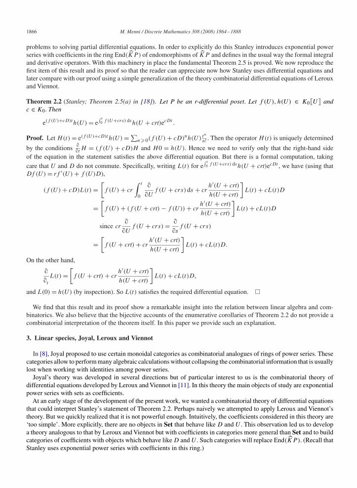
problems to solving partial differential equations. In order to explicitly do this Stanley introduces exponential powerseries with coefficients in the ring End(KP ) of endomorphisms of KP and defines in the usual way the formal integraland derivative operators. With this machinery in place the fundamental Theorem 2.5 is proved. We now reproduce thefirst item of this result and its proof so that the reader can appreciate now how Stanley uses differential equations andlater compare with our proof using a simple generalization of the theory combinatorial differential equations of Lerouxand Viennot.

Theorem 2.2 (Stanley; Theorem 2.5(a) in [18]). Let P be an r-differential poset. Let f (U), h(U) ∈ K0�U� andc ∈ K0. Then

e(f (U)+cD)th(U) = e∫ t

0 f (U+crs) dsh(U + crt)ecDt .

Proof. Let H(t) = e(f (U)+cD)th(U) =∑n�0(f (U) + cD)nh(U) tn

n! . Then the operator H(t) is uniquely determined

by the conditions ��t

H = (f (U) + cD)H and H0 = h(U). Hence we need to verify only that the right-hand sideof the equation in the statement satisfies the above differential equation. But there is a formal computation, taking

care that U and D do not commute. Specifically, writing L(t) for e∫ t

0 f (U+crs) dsh(U + crt)ecDt , we have (using thatDf (U) = rf ′(U) + f (U)D),

(f (U) + cD)L(t) =[f (U) + cr

∫ t

0

�

�Uf (U + crs) ds + cr

h′(U + crt)

h(U + crt)

]L(t) + cL(t)D

=[f (U) + (f (U + crt) − f (U)) + cr

h′(U + crt)

h(U + crt)

]L(t) + cL(t)D

since cr�

�Uf (U + crs) = �

�sf (U + crs)

=[f (U + crt) + cr

h′(U + crt)

h(U + crt)

]L(t) + cL(t)D.

On the other hand,

�

�t

L(t) =[f (U + crt) + cr

h′(U + crt)

h(U + crt)

]L(t) + cL(t)D,

and L(0) = h(U) (by inspection). So L(t) satisfies the required differential equation. �

We find that this result and its proof show a remarkable insight into the relation between linear algebra and com-binatorics. We also believe that the bijective accounts of the enumerative corollaries of Theorem 2.2 do not provide acombinatorial interpretation of the theorem itself. In this paper we provide such an explanation.

3. Linear species, Joyal, Leroux and Viennot

In [8], Joyal proposed to use certain monoidal categories as combinatorial analogues of rings of power series. Thesecategories allow to perform many algebraic calculations without collapsing the combinatorial information that is usuallylost when working with identities among power series.

Joyal’s theory was developed in several directions but of particular interest to us is the combinatorial theory ofdifferential equations developed by Leroux and Viennot in [11]. In this theory the main objects of study are exponentialpower series with sets as coefficients.

At an early stage of the development of the present work, we wanted a combinatorial theory of differential equationsthat could interpret Stanley’s statement of Theorem 2.2. Perhaps naively we attempted to apply Leroux and Viennot’stheory. But we quickly realized that it is not powerful enough. Intuitively, the coefficients considered in this theory are‘too simple’. More explicitly, there are no objects in Set that behave like D and U . This observation led us to developa theory analogous to that by Leroux and Viennot but with coefficients in categories more general than Set and to buildcategories of coefficients with objects which behave like D and U . Such categories will replace End(KP ). (Recall thatStanley uses exponential power series with coefficients in this ring.)


In this section we recall some of the work by Joyal, Leroux and Viennot and suitably generalize it for our presentpurposes. The main elementary notion is the following.

Definition 3.1. A category of coefficients is a (not necessarily symmetric) monoidal category k = (k0, ◦, I ) such thatthe underlying category k0 has finite coproducts and such that for any object C in k0, both C ◦ (_) and (_) ◦C preservefinite coproducts.

Initial objects are denoted by 0, binary coproduct is denoted by + and we will usually confuse k with the underlyingcategory k0. We speak of a symmetric category of coefficients if (k0, ◦, I ) is symmetric monoidal.

The fact that we are dealing with coproducts implies that if C + C′ is initial then so are C and C′. So, in spite ofthe notation, a category of coefficients will never be a field, neither a ring, and so we are forcing ourselves to neveruse ‘negative numbers’ in our calculations with coefficients. We see the assumption on the existence of coproducts asensuring some degree of ‘combinatorialness’ in the nature of the coefficients.

In many of the cases we will be interested in, the objects of a category of coefficients will be able to be ‘differentiated’.In order to capture this property we recall the notion of a Leibniz functor as introduced in Definition 1.8 in [14]. (Forthe notion of strength see, for example, [9].)

Definition 3.2. If k = (k0, ◦, I ) is a category of coefficients then a functor � : k0 → k0 is called a Leibniz functorif the unique map ! : 0 → �I is an isomorphism and � is equipped with strengths � : �F ◦ G → �(F ◦ G) and� : F ◦ �G → �(F ◦ G) such that [�, �] : (�F ◦ G) + (F ◦ �G) → �(F ◦ G) is an iso.

Below we will usually use the isomorphism �(F ◦ G)�(�F ◦ G) + (F ◦ �G) leaving the transformations � and �implicit.

While it is conceptually useful to have elementary definitions, we will need to assume, at certain key points (e.g.in the construction of free algebras), some non-elementary (co)completeness conditions. Mainly, that the underlyingcategories are monoidally cocomplete as defined in [7] and recalled below.

Definition 3.3. A monoidal category (k, ◦, �) is called monoidally cocomplete if it is cocomplete and moreover, thefunctors (_) ◦ C, C ◦ (_) : k → k preserve colimits for each C in k.

It is clear that every monoidally cocomplete category is a category of coefficients.

3.1. Joyal’s catégorie des espèces linéares

Let L be the (essentially small) category of finite linear orders and monotone bijections between them. This categoryis equivalent to the discrete category determined by the set of natural numbers, but it is sometimes convenient to usethe whole of L. For each k ∈ N denote the total order {0 < 1 < · · · < k − 1} by [k]. The category L can be equippedwith a (non-symmetric) monoidal structure (L, ⊕, ∅) where ⊕ is determined by the condition [k] ⊕ [k′] = [k + k′].

The category [L, Set] is complete and cocomplete and from general considerations about completeness, Day’s well-known convolution construction (see [7]) produces, out of the monoidal structure (L, ⊕, ∅), a new monoidal structure([L, Set], ∗, q0) on the category of functors from L to Set. (The notation for the unit of this monoidal structure willbecome clear in the rest of the section.) The resulting symmetric monoidal category was called catégorie des espèceslinéares in [8]. We will denote it by J.

In order to discuss the combinatorial intuition of J we first recall Joyal’s more explicit description of the tensorF ∗ G of two objects F and G in [L, Set]. (Readers unfamiliar with Day’s convolution construction can use the explicitdescription in Proposition 3.4 as the definition of J.) A cut of a linear order l is a partition l = l0l1 of l such that l0 is aninitial segment of l and l1 is a terminal segment of l. (We stress that (∅, ∅) is the unique cut of the empty linear order ∅.)

Proposition 3.4. For any F, G in [L, Set],(F ∗ G)l�

∑(l0,l1)

F l0 × Gl1


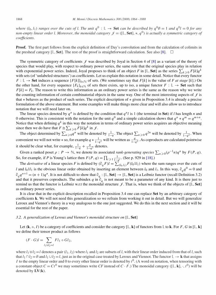
where (l0, l1) ranges over the cuts of l. The unit q0 : L → Set can be described by q0∅ = 1 and q0l = 0 for anynon-empty linear order l. Moreover, the monoidal category J = ([L, Set], ∗, q0) is actually a symmetric category ofcoefficients.

Proof. The first part follows from the explicit definition of Day’s convolution and from the calculation of colimits inthe presheaf category [L, Set]. The rest of the proof is straightforward calculation. See also [8]. �

The symmetric category of coefficients J was described by Joyal in Section 4 of [8] as a variant of the theory ofspecies that would play, with respect to ordinary power series, the same role that the original species play in relationwith exponential power series. Indeed, Joyal proposes to think of an object F in [L, Set] as the series

∑k �0 F [k]qk

with sets (of ‘unlabeled structures’) as coefficients. Let us explain this notation in some detail. Notice that every functorF : L → Set induces a sequence {F [k]}k∈N of sets. (We sometimes say that F [k] is the value of F at stage [k].) Onthe other hand, for every sequence {Fk}k∈N of sets there exists, up to iso, a unique functor F : L → Set such thatF [k] = Fk . The reason to write this information as an ordinary power series is the same as the reason why we writethe counting information of certain combinatorial objects in the same way. One of the most interesting aspects of J isthat ∗ behaves as the product of such series. The explicit description of ∗ given in Proposition 3.4 is already a preciseformulation of the above statement. But some examples will make things more clear and will also allow us to introducenotation that we will need later on.

The linear species denoted by qn is defined by the condition that qnl is 1 (the terminal in Set) if l has length n and0 otherwise. This is consistent with the notation for the unit q0 and a simple calculation shows that qn ∗ qm = qm+n.Notice that when defining qk in this way the notation in terms of ordinary power series acquires an objective meaningsince then we do have that F�

∑k �0 F [k]qk in J.

The object determined by∑

n�0qn will be denoted by 1

1−q. The object

∑n�0 q2n will be denoted by 1

1−q2 . When

convenient we will not write ∗ so, for example q ∗ 11−q2 will be written as q

1−q2 . As coproducts are calculated pointwise

it should be clear what, for example, 11−q

+ q

1−q2 denotes.

Given a ranked poset � : P → N, we denote its associated rank-generating species∑

n�0(�−1n)qn by F(P, q).

So, for example, if P is Young’s lattice then F(P, q) =∏i �1

11−qi . (See p. 929 in [18].)

The derivative of a linear species F is defined by (�qF )l =∑(l0,l1)

F (l01l1) where the sum ranges over the cuts of

l and l01l1 is the obvious linear order obtained by inserting an element between l0 and l1. In this way, �qq0 = 0 and

�qqn+1 = (n + 1)qn. It is not difficult to show that �q : [L, Set] → [L, Set] is a Leibniz functor (recall Definition 3.2)and that it preserves coproducts. The subindex q in �q is not meant to be a parameter of any kind. It is there just toremind us that the functor is Leibniz w.r.t the monoidal structure J. That is, when we think of the objects of [L, Set]as ordinary power series.

It is clear that in the explicit description recalled in Proposition 3.4 one can replace Set by an arbitrary category ofcoefficients k. We will not need this generalization so we refrain from working it out in detail. But we will generalizeLeroux and Viennot’s theory in a way analogous to the one just suggested. We do this in the next section and it will beessential for the rest of the paper.

3.2. A generalization of Leroux and Viennot’s monoidal structure on [L, Set]

Let (k, ◦, I ) be a category of coefficients and consider the category [L, k] of functors from L to k. For F, G in [L, k]we define their tensor product as follows

(F · G)l =∑

l1�l2=l

F l1 ◦ Gl2,

where l1 � l2 = l denotes a pair (l1, l2) where l1 and l2 are subsets of l, with their linear order induced from that of l, suchthat l1 ∩ l2 =∅ and l1 ∪ l2 = l, just as in the original case treated by Leroux and Viennot. The functor L → k that assignsI to the empty linear order and 0 to every other linear order is denoted by t0. (A word on notation, when tensoring witha constant object C = Ct0 we may sometimes write CF instead of C · F .) The monoidal category ([L, k], ·, t0) will bedenoted by LV(k).


Proposition 3.5. If k is a category of coefficients then LV(k) is also a category of coefficients. If the former is symmetricthen so is the latter.

Proof. Straightforward. See also [11]. �

For an arbitrary category of coefficients k, and F and G in LV(k), F ·G at stage [k] gives∑k

i=0

(ki

)(F [i]◦G[k− i]).

That is, the tensor · behaves as product of exponential power series. So it is fair to think of an object F in LV(k) as an

exponential power series∑

k �0F [k] tk

k! with coefficients in k. The letter t is a notational device analogous to the letterq in the case of J (recall Section 3.1). The reader should profit from all the advantage of the notation but never forgetthat we are working with combinatorial objects.

The case treated originally in [11] arises as LV(Set, ×, 1). In this case, notice that if �(_) denotes number of elements

of its argument then a simple calculation shows that �((F · G)[k]) gives∑k

i=0

(ki

)�(F [i])�(G[k − i]).

Let us look at some examples. The object t in LV(k) is defined by the condition that t is 1 (the terminal object inSet) at stage [1] and is empty everywhere else. A simple calculation shows that t · t = 2! t2

2! . That is: t · t is the initialobject at every stage different from [2] and at stage [2] it has 2! copies of the unit object I in k.

By Proposition 3.4, the monoidal category J is a symmetric category of coefficients. So we can consider, byProposition 3.5, the symmetric category of coefficients LV(J). An interesting example of an object in this category is

the object∑

k �0k!( 11−q

)k tk

k! which we should denote by 1

1− 11−q

t.

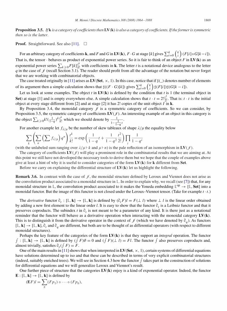
For another example let f�/� be the number of skew tableaux of shape �/� the equality below∑k

(∑n

(∑f�/�

)qn

)tk

k! = exp

(1

1 − qt + 1

1 − q2

t2

2!)∏

i

1

1 − qi

(with the unlabeled sum ranging over �/� � k and � � n) is the pale reflection of an isomorphism in LV(J).The category of coefficients LV(J) will play a prominent role in the combinatorial results that we are aiming at. At

this point we still have not developed the necessary tools to derive them but we hope that the couple of examples abovegive at least a hint of why it is useful to consider categories of the form LV(k) for k different from Set.

Before we carry on explaining the differential structure of LV(k) let us highlight the following.

Remark 3.6. In contrast with the case of J, the monoidal structure defined by Leroux and Viennot does not arise asthe convolution product associated to a monoidal structure in L. In order to explain why, we recall (see [7]) that, for anymonoidal structure in L, the convolution product associated to it makes the Yoneda embedding Lop → [L, Set] into amonoidal functor. But the image of this functor is not closed under the Leroux–Viennot tensor. (Take for example t · t .)

The derivative functor �t : [L, k] → [L, k] is defined by (�tF )l = F(⊥ l) where ⊥ l is the linear order obtainedby adding a new first element to the linear order l. It is easy to show that the functor �t is a Leibniz functor and that itpreserves coproducts. The subindex t in �t is not meant to be a parameter of any kind. It is there just as a notationalreminder that the functor will behave as a derivative operation when interacting with the monoidal category LV(k).This is to distinguish it from the derivative operator in the context of J (which we have denoted by �q ). As functors[L, k] → [L, k], �t and �q are different, but both are to be thought of as differential operators (with respect to differentmonoidal structures).

Perhaps the key feature of the categories of the form LV(k) is that they support an integral operation. The functor∫ : [L, k] → [L, k] is defined by (∫

F)∅ = 0 and (∫

F)(⊥ l) = F l. The functor∫

also preserves coproducts and,almost trivially, satisfies �t (

∫F) = F .

One of the main results in [11] shows that when interpreted in LV(Set, ×, 1), certain systems of differential equationshave solutions determined up to iso and that these can be described in terms of very explicit combinatorial structures(indeed, suitably enriched trees). We will see in Section 4.3 how the functor

∫takes part in the construction of solutions

for differential equations and we will generalize Leroux and Viennot’s result.One further piece of structure that the categories LV(k) enjoy is a kind of exponential operator. Indeed, the functor

E : [L, k] → [L, k] is defined by

(EF)l =∑�

(Fp1) ◦ · · · ◦ (Fpk),


where � ranges over the partitions of the set underlying l and p1 < p2 < · · · < pk are the components of � eachcomponent with the total order inherited from l and ordered among them according to their least element. (In the trivialcase this should be understood as saying that (EF)∅ = t0.)

(A word on notation. We will sometimes write∏

in order to refer to a finite indexed tensor, not necessarily cartesianproducts. So, for example, we can write (EF)l =∑

�∏

p∈�Fp. The underlying monoidal structure will be clear fromthe context.)

If (k, ◦, I ) is symmetric then there is a natural iso E(F + G)�EF · EG. But there is no such iso in general. On theother hand, there is a natural iso �t (EF)�(�tF ) · (EF) even if k is not symmetric.

(It seems relevant to mention that in Section 5 of [11], expressions of the form e with being certain operatorsacting on functors Ln → Set are considered. This clearly involves an idea similar to the ones in this section; but wehave not explored the precise relation.)

For F in LV(k) define 11−F

at stage l by∑

�(Fp1) ◦ · · · ◦ (Fpk) where sum ranges over the ordered partions� = {p1 < p2 < · · · < pk} and, as in the case of E, each component considered with the order inherited from l.

The object 11−t

built using the definition above is explicitly described by∑

k �0k! tkk! . This one is a good example

of a little ‘danger’ of the notation in terms of power series. The reader should resist the temptation of canceling thek!’s. The object 1

1−thas, at stage [l], l! elements. So do not confuse 1

1−twith the object 1

1−qintroduced in Section

3.1. As functors L → Set they are different. But when they interact with other objects using the monoidal structuresLV(Set, ×, 1) and J, respectively, then they behave in some ways as the function x �→ 1

1−x. Hence the notation.

3.3. Pushing coefficients forward along functors

The present short section introduces a couple of simple results that will be used throughout the rest of the paper. LetC,D and E be categories and let : D → E be a functor. Then there is a functor ∗ : [C,D] → [C,E] that assignsto each F : C → D the composite functor F : C → E.

Lemma 3.7. Let k and k′ be categories of coefficients and let : k0 → k′0 be a functor then

(1) there is a natural iso �t∗�∗�t ;(2) if preserves initial object then there is a natural iso ∗

∫�∫

∗;(3) if is a monoidal and preserves finite coproducts then ∗ is also monoidal LV(k) → LV(k′). If the categories

of coefficients and are symmetric then so is ∗. Moreover, there is a natural isomorphism ∗ E�E ∗.

Proof. Straightforward, but we prove preservation of E as an example. Using that is monoidal and that it preservescoproducts we have, for each n and � ranging over the partitions of n, that

∑�

∏p∈�

Fp�∑�

∏p∈�

(Fp)

so that ((EF)n) = (E(∗F))n. �

We will need also a variant Lemma 3.7 taking care of the case when is �q : J → J which does preservecoproducts but which is not monoidal. To avoid any possible confusion let us stress that �q∗ = (�q)∗.

Lemma 3.8. For any F in LV(J), �q∗(EF)�(�q∗F) · EF .

Proof. We let F =∑kfk

tk

k! and calculate:

(�q∗(EF))n =∑�

�q

∏p∈�

fp =∑�

∑p∈�

(�qfp) ∗∏

t∈�/p

ft

=∑a

(�qfa ∗

∑�

∏s∈�

fs

)= ((�q∗F) · EF)n,


where � ranges over the partitions of n, a over subsets of n and � over the partitions of n/a in all cases with the inducedorder. �

3.4. The combinatorial meaning of h(q) �→ h(q + crt)

The equality e(f (U)+cD)th(U) = e∫ t

0 f (U+crs) dsh(U + crt)ecDt stated in Stanley’s theorem involves ordinary powerseries f (U) and h(U) in K0�U�. On the left hand side, h(U) is used as constant exponential power series but on theright, the exponential series h(U + crt) is not constant. Moreover, it is clear from the proof of Theorem 2.2 that thebehavior of h(U + crt) plays an important role.

Although we still have not explained how we will interpret U , there is an important part of the assignment h(U) �→h(U + crt) that we can explain combinatorially at this point. First we need a somewhat abstract construction.

Let k = (k0, ◦, I ) be a category of coefficients and let : k0 → k0. For any fixed non-negative integers c, r , definethe functor +crt : k0 → [L, k0] as follows:

(+crth)[k] = (cr)kkh,

for any h in k. (Here, k denotes the composition of with itself k times. If k = 0 then k = id.) We now state twosimple properties of +crt that will be useful in Section 5.4. The first one is a ‘corecursive’ description of +crt .

Lemma 3.9. For any f in k, +crtf = f t0 + cr∫(+crtf ).

Proof. Straightforward. �

The second property concerns the behavior of +crt followed by �t .

Lemma 3.10. For any h in k, �t (+crth) = cr+crt (h).

Proof. Calculate: (�t (+crth))[k] = (cr)k+1k+1h = cr(cr)kk(h) = (cr+crt (h))[k] �

This is meant to be applied to the Leibniz functor �q : [L, Set] → [L, Set] in order to obtain a functor �q+crt:

[L, Set] → [L, [L, Set]] which, although is not monoidal, we choose to think of it as a functor J → LV(J) in thesense that it takes a combinatorial ordinary power series and produces an exponential one (with coefficients in J). So

that �q+crth =∑

k �0(cr)k�k

qh tk

k! for any h in J.For example,

�q+crt

1

1 − q=∑k �0

ckrk

⎛⎝∑n�0

(n + k)!n! qn

⎞⎠ tk

k! .

We see the functor �q+crtas providing a combinatorial interpretation of the assignment h(q) �→ h(q + crt). In

Section 5.4 it will be used to explain the meaning of the assignment h(U) �→ h(U + crt) needed to understandStanley’s result.

4. Combinatorial functional and differential equations

Let us discuss in some more detail how we deal with differential and functional equations. A standard way to interpretdifferent types of equations and their solutions in general categories is through the use of algebras for endofunctors. Letus recall the main definitions. If F : C → C is an endofunctor then an F-algebra is a pair (X, x) where X is an objectof C and x : FX → X is a map in C. Given F-algebras (X, x) and (Y, y) a morphism of algebras g : (X, x) → (Y, y)

is a map g : X → Y such that g x = y (Fg). Algebras and their morphisms can be organized into a category AlgF . Theintuition is that an equation gives rise to an endofunctor F and that a solution to the equation is an F-algebra that is afixed point of F, that is, an F-algebra (X, x) such that x is an isomorphism. The result known as Lambek’s lemma states


that the initial object of AlgF is a fixed point for F and so it is reasonable to think of this algebra (when it exists) as the‘least’ fixed point for F.

Initial F-algebras need not always exist but they do under fairly general hypotheses as the following well knownresult shows.

Lemma 4.1. If C is cocomplete and F : C → C preserves directed colimits then the category AlgF has an initialobject.

Proof. The underlying object of the initial algebra is the colimit of the �-chain 0 → F0 → · · · → F i0 → · · · . Wedenote the colimit by �F . Using preservation of directed colimits it is easy to obtain a map F�F → �F . The universalproperty of �F implies that the F-algebra just obtained is initial. �

For concrete cases of Lemma 4.1 see [1] which deals with finitary endofunctors on Set, the ‘existence’ part of theimplicit species theorem of Section 5.2 of [8] and the construction of solutions of differential equations in [11]. Now,in the last two cases there is another important phenomenon going on which is important to abstract.

Definition 4.2. A functor F : C → C is special if AlgF has an initial object and moreover for every F-algebra A, A isa fixed point of F if and only if A is initial.

This captures the unicité des solutions of the implicit species theorem in [8] and the last part of Theorem 3.1 in[11]. It is this property that allows the following kind of argument: to prove that two objects are isomorphic, just provethat the two objects are fixed points for a special functor. Notice that this is the argument displayed (at the level ofequations) in Theorem 2.2. Our strategy to give a combinatorial interpretation of Stanley’s theory is then to prove thatthere are categories of combinatorial objects on which Stanley’s differential and functional equations induce specialfunctors in the sense of Definition 4.2. In this way Stanley’s statements remain mainly unchanged. The proofs will haveto be modified because the statements will be referring to objects and morphisms in categories with coproducts. Butwe hope that the reader will agree that the spirit of Stanley’s proofs is also preserved.

Leroux and Viennot note in page 213 of [11] that the canonical solutions for the systems of differential equations“remain at certain ‘recursive’ level. This is the price to pay for a general method that works for any system of differentialequations”. Naturally, our generalization will have to pay the same price.

Remark 4.3. The definition of special functor has an existence and a uniqueness part. So it is fair to ask if it is worthfocusing on the more general notion of a functor such that every fixed point is initial in the category of algebras. Webelieve that the generalization is not useful. The reason is that, if the functor has an initial algebra then the functor isspecial. If it does not have an initial algebra, then the condition fixed-point implies initial means that there are no fixedpoints. So there is not much use for it.

Essentially, the Théorème des espèces implicites in [8] says that certain functors F : Fr → Fr are special. The mainauxiliary notion in the proof of this theorem is that of contact.

Definition 4.4. For f : A → B in [L, k] and F : [L, k] → [L, k] define

(1) f is a contact at n if fn : A[n] → B[n] is an iso.(2) f is a contact of order n if it is a contact at m for every m�n.(3) F preserves contacts if for every contact at n, F is also a contact at n.(4) F raises contacts if for every contact at n , F is a contact at n + 1.

For example, if F : [L, k] → [L, k] preserves small coproducts, then F preserves contacts. The integral∫ : [L, k] →

[L, k] raises contacts.In order to state the following result more clearly, let us define a functor F : [L, k] → [L, k] to be constant at ∅

(with coefficient K) if there exists a K in k such that for every A in [L, k], (FA)∅ = K and for every map f : A → B

in [L, k], (Ff )∅ = idK : K → K .


Proposition 4.5. Let F : [L, k] → [L, k] be such that AlgF has an initial object. If F is constant at ∅ and raisescontacts then F is special.

Proof. For the purpose of the proof assume that F is constant at ∅ with coefficient K. Let � : FA → A be the initialF-algebra and let � : FB → B is an isomorphism. We need to show that the unique map u : (A, �) → (B, �) is aniso. We do this by showing that u is a contact at n for every n, by induction. At stage ∅ we have the following diagram

K = (FA)∅ �∅−→ A∅

id=(Fu)0

⏐⏐⏐⏐⏐� u∅

⏐⏐⏐⏐⏐�K = (FB)∅ −→

�∅B∅

in other words, u∅ �∅ = �∅. As both �∅ and �∅ are isos, so is u∅.At stage n + 1 we have un+1 �n+1 = �n+1 (Fu)n+1. By inductive hypothesis, un is an iso and as F raises contacts,

(Fu)n+1 is an iso. As � and � are isos, un+1 is an iso. �

It is important to notice that the proof of Proposition 4.5 actually constructs an explicit isomorphism. At the time ofapplying the proposition, the resulting explicit iso may not be at all transparent. But we have the certainty that withsome patience and attention we will be able to extract a recursive program out of the proof above.

4.1. Examples of functional equations in J

We can think of an endofunctor F : C → C as determining a functional equation y = Fy. Fixed points can bethought of as solutions and the initial algebra as the ‘minimal’ solution. If F is special, there is essentially one solution.Let us look at some examples in the monoidal category J = ([L, Set], ∗, q0) described in Section 3.1.

Example 4.6. As the functor q∗(_) : [L, Set] → [L, Set] preserves all colimits, the functor H1 =q0 +q∗(_) preservesdirected colimits. It is easy to check that it raises contacts so the functor H1 is special. It is also easy to calculate theinitial algebra �H1 of H1. Indeed, �H1 = 1

1−q. �

The following variant of the example above will be also useful.

Example 4.7. The functor H2 = q0 + q2 ∗ (_) is special and its initial algebra �H2 can be described as 11−q2 .

Example 4.8. Consider the functor H1,l : [L, Set] → [L, Set], for a fixed linear order l > 0, defined by

H1,lX =⎛⎝∑

l0⊂l

(q

1 − q

)l0

⎞⎠+ ql ∗ X

for any X in J. Since ql ∗ (_) preserves all colimits and H1,l is obtained by adding a constant, it follows that the latterfunctor preserves all directed colimits. So the functor must have an initial algebra. As ql ∗ (_) raises contacts, so doesH1,l and hence H1,l is special. Calculating the colimit of the canonical �-chain associated with H1,l may not be as easyas in the case of Example 4.6. But the functor is special so in order to get a picture of what the initial algebra lookslike we just need to find a fixed point for it. We claim that the object ( 1

1−q)l of weak l-compositions can be given the

structure of a fixed point. Indeed there is an obvious isomorphism H1,l(1

1−q)l → ( 1

1−q)l as below⎛⎝∑

l0⊂l

(q

1 − q

)l0

⎞⎠+(

q

1 − q

)l

−→(

1

1 − q

)l

,

which reflects the fact that a partitions of length l can be split in those that have all components non-empty (i.e. ( q1−q

)l)and those that have some components empty.


Example 4.8 shows how to obtain ( 11−q

)l as the solution to a non-trivial functional equation. For different variationsinvolving r-differential posets we will need also the following variant. The proofs that the functor involved is specialand that the initial algebra is what it should be are non-problematic variants of Example 4.8.

Example 4.9. For a fixed linear order l > 0, non-negative integer r and fixed K inJ consider the functor H : [L, Set] →[L, Set] defined by

HX = l!rl

⎛⎝∑l0⊂l

(q

1 − q

)l0

⎞⎠ ∗ K + ql ∗ X

for any X inJ. The functor H is special for the same reasons that H1,l is (see Example 4.8). We claim that l!rl( 11−q

)l ∗K

is a fixed point for H . In fact, this follows easily using that tensoring with l!rlK distributes over coproducts and usingthe fixed point structure described in Example 4.8.

4.2. The functor Q and further functional equations

Let us look at another example. This time, in the category LV(J) determined by J and Proposition 3.5. First wedefine the functor Q : [L,J] → [L,J] as follows

Q

⎛⎝∑k �0

pk

tk

k!

⎞⎠=∑k �0

qk ∗ pk

tk

k! ,

where pk in J for every k.

Lemma 4.10. The functor Q is cocontinuous, monoidal and preserves exponentials.

Proof. Cocompleteness follows because colimits are calculated pointwise in [L,J] and because tensoring with qk iscocontinuous. The rest is straightforward calculation. �

We are interested in the functor Et · Q : [L,J] → [L,J] but since it preserves initial object then we cannot applyexactly the same argument as in the previous cases. To deal with the present case fix an object K in J and considerthe subcategory C of [L,J] determined by those objects X such that X∅ = K and those morphisms f : X → Y suchthat f∅ = idK . The object K is initial in C so the functor Et · Q does not preserve initial object when restricted to C.Obviously the inclusion C → [L,J] does not preserve the initial object either. But it should be clear that the inclusioncreates directed colimits. So the colimits (in C) involved in the construction of free algebras are calculated as in [L,J].It follows that Et · Q : C → C preserves directed colimits. (The idea of building a category with a different initialobject is also what accounts for functional equations with an initial condition.)

Proposition 4.11. The functor Et · Q is special when restricted to the category C. Its initial algebra can be describedas E( 1

1−qt)K .

Proof. Denote the functor in the statement by T so that T X = Et · QX. The discussion above implies that T has aninitial algebra. To describe it let An = E((

∑ni=0q

i)t)K and then, using that Q preserves exponentials, it follows thatT An = An+1. Moreover, T K = (Et)K = A0. So that, at stage l we have the colimit diagram:

A0l −→ A1l · · · −→ Anl −→ · · · −→ (�T )l,

which reduces to the following diagram

(q0)l ∗ K −→ (q0 + q)l ∗ K −→(

n∑i=0

qi

)l

∗ K −→ · · · −→ (�T )l

in J. A simple argument shows that (�T )l = ( 11−q

)l ∗ K so we can conclude that �T = E( 11−q

t)K .We must show that T is special. So assume that we have a fixed point � : T B → B. We claim that for each l,

Bl = ( 11−q

)l ∗ K . We prove this by induction. The base case is trivial because B∅ = K . So assume that l �= ∅ and then


notice that

(Et · QB)l =∑

l0,l1⊆l

(Et)l0 ∗ (QB)l1 =∑l1⊆l

ql1 ∗ Bl1

so (Et · QB)l = (∑

l1⊂lql1 ∗ ( 1

1−q)l1 ∗ K) + ql ∗ (Bl) by induction. But then �l is essentially providing Bl with a fixed

point structure for the functor H1,l of Example 4.8 (actually, a variant tensoring with constant K as in Example 4.9).As this functor is special, it must be the case that Bl�( 1

1−q)lK . �

Using the same ideas as in Proposition 4.11 one proves the following result (we leave the details to the reader).

Proposition 4.12. The functor E(rt + r t2

2 ) · Q : C → C is special and its initial algebra can be described as

E( r1−q

t + r1−q2

t2

2 ) · K .

We need one more example which we discuss in more detail. The category [L, k] has another symmetric monoidalstructure which can be described by

(F ⊗ G)l =∑

l0+l1=ll′0+l′1=l

F l0 ◦ Gl1,

where the cardinalities of li and l′i coincide for i equal to 0 or 1. The idea is to think of an object in [L, k] as a series∑k �0ak

tk

k!2 and then⎛⎝∑k �0

ak

tk

k!2

⎞⎠⊗⎛⎝∑

k �0

ak

tk

k!2

⎞⎠=∑

k

(k∑

i=0

(k

i

)2

aibk−i

)tk

k!2 .

But we will not need to go deeper into this monoidal structure. We just need to tensor with a constant.

Proposition 4.13. The functor 11−t

⊗ Q(_) is special when restricted to C and its initial algebra can be described as1

1− 11−q

t· K .

Proof. This is similar to Proposition 4.11 but we go through some of the details. We denote the functor in the statementby T so that T X = 1

1−t⊗ QX. If we let An = 1

1−(∑n

i=0qi )t

K then it is easy to prove that T An = An+1. Moreover,

T K = 11−t

K = A0. In other words, we have that Anl = l!(∑ni=0q

i)lK and so, much as in Proposition 4.11, we can

conclude that (�T )l = l!( 11−q

)lK and hence that �T = 1

1− 11−q

tK .

We must show that T is special. So assume that we have a fixed point � : T B → B. We claim that for each l,Bl = l!( 1

1−q)lK . We prove this by induction. The base case is trivial because B∅ = K . So assume that l �= ∅ and then

notice that(1

1 − t⊗ QB

)l =

l∑i=0

(l

l − i

)2

(l − i)!qi ∗ Bi

=(

l−1∑i=0

(l

l − i

)2

(l − i)!qi ∗ Bi

)+ ql ∗ Bl

so that by induction(t

1 − t⊗ QB

)l =

(l−1∑i=0

(l

l − i

)2

(l − i)!i!qi ∗(

1

1 − q

)i

K

)+ ql ∗ Bl

= l!(

l−1∑i=0

(l

i

)(q

1 − q

)i)

K + ql ∗ Bl,


but then �l is essentially providing Bl with a fixed point structure for the functor H of Example 4.9 (with r = 1). Asthis functor is special, it must be the case that Bl�l!( 1

1−q)lK . �

It should be clear how to modify the above for the case r > 1.

4.3. Differential equations reduced to functional equations

Following [11] we explain here how to produce solutions to differential equations using Proposition 4.5. We onlyneed the case of one equation so we restrict to that case. For us, a differential equation in LV(k) is given by a functorG : [L, k] → [L, k] and an object K in k. We think of this data as expressing the equation �t y = Gy with initialcondition y∅ = K .

Lemma 4.14. Let G preserve contacts. If F is defined by FA = K + ∫GA then it is constant at ∅ and raises contacts.

Proof. Assume that is a contact at n. Then

(F)n+1 = idK +(∫

G

)n+1

= idK + (G)n.

As G preserves contacts (G)n is an iso. So (F)n+1 is an iso. �

So, if in the situation above it also happens that AlgF has an initial object (e.g. if G preserves directed colimits) thenF is special by Proposition 4.5. The relation with differential equations was described by Leroux and Viennot in Section3 of [11]: there is an iso K + ∫ GA�A if and only if A∅�K and �A�GA. So, in the notation of the previous lemma,the initial algebra for F is the solution to the combinatorial differential equation �y = Gy with boundary conditiony∅ = K .

Example 4.15 (Leroux and Viennot [11] Example 4.1). The essentially unique solution to the differential equation�t y = t0 + y · y with initial condition y∅ = ∅ in the category LV(Set, ×, 1) can be described as complete increasingbinary trees or as alternating descending odd permutations.

Example 4.16 (Leroux and Viennot [11] Example 4.3). The differential equation �t y = 11−y

with initial conditiony∅ = ∅ has a solution which can be described as increasing planar trees.

Some of the main results of the present paper will rely on the following class of examples.

Example 4.17. Let k be a cocomplete category of coefficients and let K and L be non-initial objects of k. We considera differential equation in the category LV(k). If tensoring with K induces a cocontinuous functor [L, k] → [L, k] (asit does in our examples), the differential equation �t y = K · y with initial condition L has a unique solution. We canthen conclude that the solution E(Kt)L is the solution for this differential equation.

Remark 4.18. It seems relevant to mention that there exists also a theory of combinatorial differential equations forJoyal’s ordinary species which has a completely different flavor from that by Leroux and Viennot. See for example[10] and [15].

5. Weyl categories

As recalled in the introduction, Stanley starts with a field K0 of characteristic 0 and denotes the field of Laurent serieswith coefficients in K0 by K. He then defines the K-vector space KP of arbitrary linear combinations

∑x∈P cxx with

cx ∈ K and introduces exponential power series with coefficients in the ring End(KP ) of endomorphisms of KP . HisTheorem 2.5 is a statement about such exponential power series.

Our combinatorial interpretation of Theorem 2.2 requires the construction of a suitable category of coefficients thatwill play the role that End(KP ) plays in Stanley’s formulation. But key portions of the proofs rely only in simple


algebraic properties so we believe that it is convenient to capture these properties in a way that it is independent of theircombinatorial manifestations. One way of doing this is through down-up algebras as in [2]. We will insist on requiringcategorical coproducts.

Definition 5.1. Let r be a positive integer. A category of coefficients (W, ◦, I ) is called an r-Weyl category if it isequipped with a choice of two objects D and U in W and morphisms �0 : U ◦ D → D ◦ U and �1 : rI → D ◦ U

such that the morphism [�0, �1] : U ◦ D + rI → D ◦ U is an isomorphism.

IfW is an r-Weyl category then we will just use juxtaposition instead of ◦; in this way we can rewrite the isomorphismin Definition 5.1 as DU�UD + rI .

Remark 5.2. The terminology is obviously intended to make reference to Weyl algebras. Indeed, the complex associa-tive algebra generated by elements d and u subject to the relation du − ud = 1 is the Weyl algebra sometimes denotedby A1. As explained in [3], there is a natural action of A1 on C[x] defined by d · P(x) = P ′(x) and u · P(x) = xP (x)

and this establishes an isomorphism of A1 with the algebra of differential operators with polynomial coefficients (inone variable). Of course, the condition du − ud = 1 is just a manifestation of the Leibniz rule and as explained in theintroduction we will think of D as �/�U .

Notice that the requirement (in Definition 5.1) of + being categorical coproduct prevents rings from being examplesof Weyl categories. But it is not surprising that for many identities valid in A1 (not involving −) there are analogousisomorphisms in Weyl categories. There are probably deeper connections between Weyl categories and Weyl algebrasbut we will not attempt to pursue them here.

In this section we establish a number of basic facts about Weyl categories and we associate to every poset P a categoryof coefficients WP equipped with a canonical choice of objects D and U . This choice of objects extends to an r-Weylcategory structure on WP if and only if P is r-differential. This result is, of course, analogous to Theorem 2.2 in [18].

Under a suitable completeness hypothesis on an r-Weyl category W we will be able to solve combinatorial andfunctional equations in LV(W) and prove a result analogous to Theorem 2.2 which, applied to the case W=WP willprovide the combinatorial information obtained by Stanley.

Let W be an r-Weyl category. When seen as constant objects in LV(W), D and U provide this category with anr-Weyl structure. Whenever we consider a category of the form LV(W) we will assume that it is equipped with thisWeyl structure.

5.1. The Weyl categories of operators

As we have already explained, our version of Stanley’s theorem replaces the ring End(KP ) with a suitably cocompleteWeyl category (Definition 5.1). But naturally, in order to derive concrete enumerative corollaries, concrete Weylcategories will have to be used. In this section we build such categories relying on well-known analogies between linearmaps and cocontinuous functors.

Think of the category Set as K. If we let |P | be the underlying set of the poset P then [|P |, Set] should be thoughtof as KP . Indeed, a functor |P | → Set is essentially a family of sets indexed by |P | and we will sometimes write∑

x∈P ax with ax in Set for an object in this category (and may even speak of vectors). Because of this we denote thecategory [|P |, Set] by P .

The natural next step is to consider the category of cocontinuous functors P → P as an alternative to the ringEnd(KP ). This is essentially what we will do. But in order to have a category that is easier to visualize, we will relyon categorical results (using Kan extensions) which allow to describe such functors in more concrete terms. Readersunfamiliar with Kan extensions can simply take the monoidal categories WP = ([|P × P |, Set], ◦, �) described belowas combinatorial alternatives to End(KP ).

For A, B : |P × P | → Set we define

(B ◦ A)(x, y) =∑t∈P

A(x, t) × B(t, y)

and �(x, y)=1 if x=y and �(x, y)=∅ if x �= y. With these definitions the proof of the following result is straightforward.


Lemma 5.3. For any poset P, the structure WP = ([|P × P |, Set], ◦, �) is a monoidally cocomplete (non-symmetric)monoidal category.

We now introduce objects U and D in WP . The object U is determined by defining that U(x, y) is the singleton 1if y covers x and it is ∅ otherwise. The object D is defined by declaring D(x, y) to be the singleton if x covers y and tobe empty otherwise. In other words, U(x, y) = D(y, x).

Lemma 5.4. For any poset P, the following hold:

(1) DU(x, y) = x+ ∩ y+(2) UD(x, y) = x− ∩ y−

Proof. For the first item just calculate

DU(x, y) =∑t∈P

U(x, t) × D(t, y)�x+ ∩ y+.

The second item is analogous. �

Before we state the next result let us make a short comment on axioms (D2) and (D3). As stated in [18] andreproduced in Section 1 these axioms state that certain pairs of finite sets have the same number of elements. Withoutbeing very explicit about it we are going to assume that the axioms actually provide concrete isomorphisms. Forexample, (D3) should provide for each x in P an isomorphism x− + r → x+. (Compare with the R-correspondencesas in Definition 2.6.1 in [16].) With this in mind let us state a result analogous to Theorem 2.2 in [18].

Theorem 5.5. Let P be a poset and r be a positive integer. Then P satisfies (D2) and (D3) if and only if the objects D

and U extend to an r-Weyl structure on WP .

Proof. We need to define an iso DU(x, y) → UD(x, y)+r�(x, y). From Lemma 5.4 we see thatAxiom (D2) providesthe iso in the case when x �= y and axiom (D3) provides the iso when x = y. �

In order to exemplify the combinatorial importance of the operators D and U Stanley highlights the followingexamples. (Although the lemma below is not stated as such, its content follows from Proposition 3.1 in [18] and thediscussion following it.)

Lemma 5.6. For D and U as defined above,

(1) Dn(y, x) is the set of chains x = x0 < x1 < · · · < xn = y in P such that xi covers xi−1 for each 1� i�n.(2) (U + D)n(y, x) is the set of sequences x = x0, x1, . . . , xn = y such that for each 1� i�n, either xi covers xi−1

or xi−1 covers xi .(3) DnUn(x, x) is the set of closed walks of the form

x < x1 < · · · xn−1 < xn > yn−1 > · · · > y1 > x.

Let � : P → N be a graded poset. Denote by �(n → n + k) the set of chains x0 < x1 < · · · < xk such that �x0 = n

and for each i < k, xi+1 covers xi . To discuss closed Hasse walks we denote by (n → n + k → n) the set ofHasse walks x0 < x1 < · · · < xk > xk+1 > · · · > x2k such that �x0 = n, x0 = x2k and each element is covered or iscovered by the next in the obvious way. We will denote the set of closed Hasse walks that first go down and thenup by (n → n − k → n). The notation is borrowed from [18] although notice that Stanley uses �(n → n + k) todenote the number of saturated chains while for us it is the set of such. We thought it inconvenient to introduce newnotation to stress the difference. An analogous remark holds for . Finally notice that there is an obvious isomorphism (n → n + k → n)� (n + k → n → n + k).


5.2. The combinatorial meaning of f (U)

Stanley’s Theorem 2.2 involves ordinary power series f (U) and h(U) in the ring K0�U�. In this short section weexplain how we will re-interpret such objects in the context of Weyl categories.

Let W be a monoidally cocomplete category and consider the functor L → W defined by [k] �→ Uk . It is clearlymonoidal so, as the monoidal category J is the result Day’s convolution, its universal property induces an essentiallyunique cocontinuous monoidal functor u : J → W which intuitively assigns U to q. Explicitly u(

∑n�0anq

n) =∑n�0anU

n. So, for f in J, uf will correspond to what Stanley writes as f (U).Certainly, Stanley’s notation is more intuitive but ours is more efficient in some calculations. Moreover, we will

sometimes find it useful to write uf as f . In this way, one is able to make explicit the nature of an object in a formulawithout introducing new letters. This change in notation may appear artificial at first but we hope the reader willappreciate its advantages after using it in some calculations. In the statement of the main results we will recall thenotation we introduced and relate it to Stanley’s in order to ease the reading of the paper.

5.3. Residuated functors

Corollary 2.4 in [18] states that Df (U) = rf ′(U) + f (U)D holds for every f (U) in K�U�. Stanley explains thatthe effect of this result is that we can informally view D as the derivative �

�U. Of course, there will be an analogue in

our setting. But before we state it let us introduce another relevant notion.

Definition 5.7. Let W be an r-Weyl category. A functor � : C → W is called a residuated functor if it comesequipped with a functor R : C → C and natural transformations �x : r�(Rx) → D(�x) and �x : (�x)D → D(�x)

such that [�, �] : r�(Rx) + (�x)D → D(�x) is an isomorphism. The functor R is called the residue of �. We alsosay that � is residuated by R.

Usually we will avoid writing down � and � explicitly and simply work with the iso D(�x)�r�(Rx) + (�x)D.For example, let W be a monoidally cocomplete category and consider the functor u : L → W defined in Section

5.2 in order to interpret objects in K0�U�. (Recall that for certain purposes we will denote uf by f .)

Lemma 5.8. The functor u : J → W is residuated by �q . In other words, for any f in J, Df �r�qf + f D.

Proof. Essentially the same proof of Corollary 2.4 in [18] except that we are working with isomorphisms instead ofequality. But the fact that coproducts are commutative and that tensoring on either side preserves them allows the sameproof to go through. �

The next two results allow us to build new residuated functors which, in turn, will play an important role in the proofof Theorem 6.1.

Lemma 5.9. Let � : C → W be residuated by R : C → C. If C has finite coproducts and � preserves them then thefunctor

CR+crt−→[L,C] �∗−→[L,W]

is also residuated by R.

Proof. We need an iso r�∗(R+crt (Rx)) + �∗(R+crt x)D → D�∗(R+crt x). That is: a family r�((R+crt (Rx))[k]) +�((R+crt x)[k])D → D�((R+crt x)[k]) of isos indexed by [k] ∈ L and natural in x. But (R+crt (Rx))[k]=(cr)kR(Rkx)

so, using that � preserves sums by hypothesis (and that D also does) then we need a family (cr)kr�(R(Rkx)) +(cr)k�(Rkx)D → (cr)kD�(Rkx). Hence, we have reduced the problem to finding a natural family of isomorphismsr�(R(Rkx)) + �(Rkx)D → D�(Rkx). This is provided by the assumption that � is residuated by R. �

Lemma 5.9 will be used in Section 5.4 to prove that our combinatorial interpretation of the assignment h(U) �→h(U + crt) is a residuated functor. The following lemma is almost immediate.


Lemma 5.10. Let � : C → W be residuated by R. Then �∗ : [L,C] → [L,C] is resituated by R∗ : [L,C] → [L,C].

We can use it to prove the following.

Lemma 5.11. Let � : J → W be a monoidal functor preserving finite coproducts and residuated by �q . Then

D(E(�∗F))�r(�∗�q∗F) · E(�∗F) + E(�∗F)D

for every F in LV(J).

Proof. Calculate:

D(E(�∗F)) = D�∗(EF) Lemma 3.7

= r�∗�q∗(EF) + (�∗(EF))D Lemma 5.10

= r�∗(�q∗F · (EF)) + E(�∗F)D Lemma 3.8 + Lemma 3.7

= r(�∗(�q∗F)) · E(�∗F) + E(�∗F)D Lemma 3.7. �

We will mainly be interested in the case when � = u = (_).

Corollary 5.12. For any F in LV(J),

D

(E(∫

u∗F))

�r

(∫u∗�q∗F

)· E(∫

u∗F)

+ E(u∗F)D.

Proof. Calculate:

D(E(∫

(u∗F))) = D

(E(u∗(∫

F)))

Lemma 3.7

= r(

u∗�q∗∫

F)

· E(u∗∫

F)+ E

(u∗∫

F)D Lemma 5.11

= r(∫

u∗�q∗F)

· E(∫

u∗F)+ E(u∗F)D Lemma 3.7. �

Before we move on let us give another small application of Lemma 5.11. It is taken from inside the proof ofTheorem 2.5(b) in [18] and will be used in Section 6.1.

Corollary 5.13. Let T in LV(W) be defined by T = c(r + U)t + c2r t2

2 then

DET = crt · ET + (ET )D.

Proof. Notice that T is

(cr + cU)t + c2rt2

2= u(cr + cq)t + uc2r

t2

2= u∗

((cr + cq)t + c2r

t2

2

).

Then, by Lemma 5.11, we need only to check that

�q∗

((cr + cq)t + c2r

t2

2

)= �q(cr + cq)t + (�qc2r)

t2

2= ct ,

so the result follows. �

5.4. The combinatorial meaning of h(U + crt)

In Section 3.4 we observed that the exponential series h(U +crt) appearing in Stanley’s equality e(f (U)+cD)th(U)=e∫ t

0 f (U+crs) dsh(U + crt)ecDt is not constant. We then mentioned that the functor �q+crtis a combinatorial analogue


of the assignment h(q) �→ h(q + crt) and explained that it was going to be used to give a combinatorial interpretationof the assignment h(U) �→ h(U + crt). In this section we explain how this is done.

First recall that in Section 5.2 we explained that we are going to replace statements of the form h(U) ∈ K0�U� byan object uh = h for an object h in J. Now, for monoidally cocomplete W, denote the composition

J�q+crt−→ [L,J] u∗−→[L,W]

by v : J → [L,W]. In power series notation we have, for any h inJ, that vh=∑k �0ckrku(�k

qh) tk

k! =∑

k �0ckrk�k

qh tk

k! .As in the case of u we leave r and c implicit as they will always be clear from the context. Also as in the case of u weintroduce a nameless notation to facilitate some of the calculations. Indeed we sometimes write h instead of vh. Alltold, the object h is what corresponds to h(U + crt) in our setting.

We now prove key properties of the relation between D in W and the two functors u and v. The proofs of these donot involve differential equations. For the rest of the section assume that W is monoidally cocomplete.

Corollary 5.14. For any h in J, �t (vh)�crv(�qh). That is: �t h�cr�qh.

Proof. Use �tu∗ = u∗�t (Lemma 3.7) and Lemma 3.10 applied to = �q . �

Now recall the notion of residuated functor (Definition 5.7).

Corollary 5.15. The functor v is residuated by �q . In other words: for every h in J Dh�r�qh + hD.

Proof. Use Lemma 5.8 and Lemma 5.9 applied to � = u and R = �q . �

Item 3 in Proposition 5.16 below will be essential in the proof of the main Theorem while items 1 and 2 are used toprove item 3.

Proposition 5.16. For any f in J, there are in LV(W), isos as below

(1) f �f + cr∫

�qf

(2) DE(∫

f )�r(∫

�qf ) · E(∫

f ) + E(∫

f )D

(3) (f + cD) · E(∫

f )�f · E(∫

f ) + E(∫

f )(cD).

Notice that D appears above as a constant object in LV(W).

Proof. Item 1 follows from Lemma 3.9 applied to = �q . To prove item 2 apply Corollary 5.12 to F = �q+crt. To

prove item 3 we use the same trick that Stanley uses in the proof reproduced in the introduction (see Theorem 2.2);namely we apply item 1. Indeed, we calculate as below:

f · E(∫

f

)+ E

(∫f

)(cD) =

(f + cr

∫�qf

)· E(∫

f

)+ cE

(∫f

)D item 1

= f E(∫

f

)+(

cr

∫�qf

)· E(∫

f

)+ cE

(∫f

)D

= f E(∫

f

)+ c

((r

∫�qf

)· E(∫

f

)+ E

(∫f

)D

)= f E

(∫f

)+ cDE

(∫f

)item 2

= (f + cD) · E(∫

f

). �


6. The main result

We now have all the concepts necessary to give our combinatorial interpretation of Stanley’s Theorem 2.2. The mainidea is that this result is essentially a statement about categories of the form LV(W) for an r-Weyl category W, andthat a sufficient condition for it to hold is that W be monoidally cocomplete. Stanley’s enumerative corollaries areobtained by replacing W with the category WP described in Section 5.1.

The equality e(f (U)+cD)th(U) = e∫ t

0 f (U+crs) dsh(U + crt)ecDt stated in Stanley’s theorem involves ordinary powerseries f (U) and h(U) in K0�U� which determine h(U + crt) and f (U + crs) in End(KP ).

In our interpretation, f and h are objects in J and, as explained in Section 5.2 these induce objects uf and uh in W(which are analogous to f (U) and h(U)) and which we denote by f and h to ease the main calculations. Also, f and hinduce objects vf and vh in LV(W) which, as explained in Section 5.4 are analogous to f (U + crt) and h(U + crt).(Again, we will use the nameless notation so that vf will be denoted by f and vh by h.)

Theorem 6.1. Let W be a monoidally cocomplete r-Weyl category. For any f, h in J and c ∈ N there exists anisomorphism

E((f + cD)t) · h�E(∫

f

)· h · E(cDt)

in the category LV(W).

Proof. We can first show that E((f + cD)t)�E(∫

f)

· E(cDt) and then that E(cDt) · h�h · E(cDt). In the first

case we prove that both E((f + cD)t) and E(∫

f)

· E(cDt) are solutions for �t y = (f + cD) ·y with initial condition

y∅ = I . The first object is clearly a solution, so consider the second. The initial condition is trivially satisfied. Now,using the Leibniz rule, the formula for deriving exponentials, the distributive law and finally Proposition 5.16(3) weobtain:

�t

(E(∫

f

)· E(cDt)

)= �tE

(∫f

)· E(cDt) + E

(∫f

)· �tE(cDt)

= f · E(∫

f

)· E(cDt) + E

(∫f

)· (cD) · E(cDt)

=[f · E

(∫f

)+ E

(∫f

)· (cD)

]· E(cDt)

= (f + cD) · E(∫

f

)· E(cDt),

so the theory of combinatorial differential equations provides the required isomorphism.To build the second isomorphism we show that both E(cDt) · h and h · E(cDt) satisfy the differential equation

�t y = (cD) · y with initial condition y∅ = h. Clearly, �t (E(cDt) · h) = (cD) · E(cDt) · h. On the other hand, calculate:

�t (h · E(cDt)) = �t h · E(cDt) + h · �tE(cDt)

= cr�qh · E(cDt) + h(cD)E(cDt) Corollary 5.14

= c(r�qh + hD) · E(cDt)

= c(Dh) · E(cDt) Corollary 5.15

and so, the theorem follows. �


Notice that while the proof of Theorem 6.1 follows Stanley’s strategy, all the uses of minus or division have beenremoved.

6.1. The isomorphism DP�(U + r)P

Theorem 2.5 in [18] has a second part. That is, apart from the equality e(f (U)+cD)th(U) = e∫ t

0 f (U+crs) dsh

(U + crt)ecDt , Theorem 2.5 states that under certain conditions on f (U) and h(U), the following equation

e(f (U)+cD)th(U)P = e(crt+c2rt2

2 +cUt+∫ t0 f (U+crs) ds)

h(U + crt)P

holds, where P =∑x∈P P in KP .

In this section we prove a result analogous to the one just stated. Of course, as in the case of Theorem 6.1 we needto reinterpret some of Stanley’s ideas. In his approach, D and U are operators on the vector space KP so he definesthe object P in KP and whose main property is that DP = (U + r)P holds in KP . We have decided to abstract fromthis situation and reformulate this equation as an isomorphism taking place in the ‘category of operators’. The relationbetween the two ideas will appear more explicit in Section 7.1.

Definition 6.2. Let W be an r-Weyl category. An object A in W is called switching if there exist maps UA → DA

and rA → DA such that the induced UA + rA → DA is an isomorphism.

For example, if P is a differential poset and we denote the terminal object of WP by 1 then 1 is switching. Theterminal object is concretely defined by 1(x, y) = 1 the singleton set for every (x, y) so that D1(x, y) =∑

pD(p, y)

which is the set of elements in P that cover y. Analogously, U1(x, y) is the set of elements covered by y. So, as it isobserved in Theorem 2.3 in [18], only (D3) is used to prove that 1 is switching.In order to state the following resultrecall (from Section 5.2) that if W is monoidally cocomplete then we have a functor u : J → W which intuitivelyreplaces q by U . (Recall also that for notational convenience we sometimes write f instead of uf .)

Lemma 6.3. Let W be monoidally cocomplete and A be switching in W. Then we have, in LV(W), the followingisomorphisms:

(1) Df A�r(�qf ) + (U + r)f A, for every f in J;

(2) E(cDt)A�E(c(U + r)t + c2r t2

2 )A.

Proof. The first item is a simple corollary of Lemma 5.8. (See also Corollary 2.4(b) in [18].) For the second item wefollow the proof of Theorem 2.5(b) in [18], we show that both sides of the equation are solutions to the differentialequation �t y = cDy with initial condition A. The left hand side of the equation clearly is a solution. So consider the

right hand side. The initial condition is trivially satisfied. For the non-trivial case let L = E(c(U + r)t + c2r t2

2 ). Wethen have that �tL�(c(U + r)+ c2rt) ·L�cL · ((U + r)+ crt). As we are assuming that A is switching, we have that

(U + r + crt)A = (U + r)A + crtA = DA + crtA = (crt + D)A.

Using Corollary 5.13 we can conclude that

�t (LA) = (�tL)A = cL · ((U + r) + crt)A

= cL · (crt + D)A = c(crtL + LD)A = cDLA. �

As illustration consider the following important particular case.

Example 6.4. Applying Lemma 6.3 to c = 1 and A= 1 in WP (for differential P) we obtain that E(Dt)1=E(rt+r t2

2 ) ·E(Ut) · 1.

Using Lemma 6.3 and Theorem 6.1 together we conclude the following more general result which is analogous tothe second part of Theorem 2.5 in [18].


Corollary 6.5. Let W be a monoidally cocomplete r-Weyl category with a switching object A. For any f, h in J andc ∈ N there exists an isomorphism

E((f + cD)t) · h · A�E(

c(r + U)t + c2rt2

2+∫

f

)· h · A

in the category LV(W).

7. Enumerative corollaries

In this section we discuss how to derive enumerative corollaries from Theorem 6.1. The main idea here is that ifP is r-differential then there are different functors WP → J which intuitively ‘count’ the combinatorial informationcontained in the objects of WP . In order to describe these functors it is convenient to recall a standard piece of categorytheory. Any functor f : C → D between essentially small categories induces a functor f ∗ : [D, Set] → [C, Set]which has both left and right adjoints (see Theorem I.9.4 in [13]). The functor f ∗ is defined by (f ∗H)C = H(f C) foreach H in [D, Set] and C in C. The left adjoint to f ∗ is sometimes denoted by f! and it is defined, when C and D aregroupoids (as in our case), by (f!T )D =∑

f C=DT C for each T in [C, Set] and D in D. (We will not need the rightadjoint to f ∗.)

Consider for example a graded poset P with grading � : P → N. Of course, this monotone map induces afunction � : |P | → N between the underlying sets. In this way, we obtain a functor �! : [|P |, Set] → [N, Set].Now recall from Section 5.1 that we denote the category [|P |, Set] by P and that we thought of it as analogous tothe vector space KP in Stanley’s context. Moreover, since N is equivalent to L, [N, Set] is equivalent to [L, Set]so that we choose to see �! as a functor �! : P → J that for each ‘vector’ F in P (recall Section 5), assigns theobject

�!F =∑n�0

⎛⎝∑�x=n

Fx

⎞⎠ qn,

which intuitively counts the information in F according to the levels.Another example is the second projection � : P × P → P which assigns y to each pair (x, y) in P × P . As before,

this induces a function � : |P × P | → |P | and so, a functor �! : WP → P such that to each T in WP assigns the‘vector’

�!T =∑x∈P

⎛⎝∑y∈P

T (y, x)

⎞⎠ ,

in P .For some fixed k consider the object Dk in WP . We then have that

�!�!Dk = �!

⎛⎝∑x∈P

⎛⎝∑y∈P

Dk(y, x)

⎞⎠⎞⎠=∑n�0

⎛⎝∑�x=n

∑y∈P

Dk(y, x)

⎞⎠ qn,

so Lemma 5.6 implies that (��)!Dk = �!�!Dk =∑n�0�(n → n + k)qn is an object in J counting saturated chains.

Consider now the diagonal functor � : P → P × P defined by �p = (p, p). It induces a functor �∗ : WP → P

defined by (�∗F)x = F(x, x). So, for example, �∗(DkUn) is the ‘vector’∑

x∈P DkUn(x, x) which at ‘coordinate x’counts the number of Hasse walks that start at x, go up n steps and then go down k steps finishing at x. It is then clearthat DkUn(x, x) is empty if k �= n.

Now, the main enumerative results in [18] (e.g. Theorems 3.2 or 3.11) are stated in terms of exponential power serieswith coefficients of ordinary power series. In our context, these results will be expressed as isomorphisms in LV(J)

which, in turn, will be obtained by pushing forward (in the sense of Section 3.3) certain isomorphisms in LV(WP ).


But before we obtain the isomorphisms let us look at how the combinatorial objects in question appear in the image ofa functor LV(WP ) → LV(J).

Using the notation introduced in Section 3.3 the functor (��)! : WP → J induces a functor ((��)!)∗ : LV(WP ) →LV(J). Using the observation above we can calculate

((��)!)∗E(Dt) =∑k �0

(��)!Dk tk

k! =∑k �0

⎛⎝∑n�0

�(n → n + k)qn

⎞⎠ tk

k! ,

so, in particular, counting skew tableaux amounts to finding an explicit formula for ((��)!)∗E(Dt) in the case when Pis Young’s lattice. One of the remarkable facts observed by Stanley is that in order to get such a formula the only thingwe need to know about Young’s lattice is that it is a differential poset. We will come back to this in Section 7.1.

As another example consider the object 11−q

in J and denote u( 11−q

) in WP by 11−U

. Consider also the object in

LV(WP ) given by E(Dt) 11−U

and denote it by E(Dt)1−U

. Then apply (�∗)∗ : LV(WP ) → P to obtain

(�∗)∗E(Dt)

1 − U=∑k �0

�∗(

Dk∑n

Un

)tk

k! =∑k �0

(∑n

�∗(DkUn)

)tk

k! ,

but we have just seen that �∗(DkUn) is the ‘vector’∑

x∈P DkUk(x, x) and by Lemma 5.6 we have that �!(�∗(DkUn))=∑n�0 (n → n + k → n)qn in J so

(�!)∗(

(�∗)∗E(Dt)

1 − U

)=∑k �0

⎛⎝∑n�0

(n → n + k → n)qn

⎞⎠ tk

k!

is an object in LV(J) that counts closed Hasse walks.

7.1. Counting skew shapes

In this section we prove a combinatorial analogue of Theorem 3.2 in [18] which gives a formula for countingascending chains in differential posets. As in the whole paper the idea is to be able to interpret the key ideas in [18] inour present context. The only observation we need in this case is the following.

Lemma 7.1. If P is an r-differential poset then �!F��∗(F1) for every F in WP . Moreover, this lifts to LV(WP ) and,in particular, there exists an isomorphism (�!)∗E(Dt)�(�∗)∗(E(Dt)1).

Proof. Notice that (�!F)y =∑x∈P F (x, y) = (�∗(F1))y. �

We can now prove the our analogue of Theorem 3.2 in [18].

Theorem 7.2. If � : P → N is a graded r-differential poset then there is an iso

∑k �0

⎛⎝∑n�0

�(n → n + k)qn

⎞⎠ tk

k!�E(

r

1 − qt + r

1 − q2

t2

2

)F(P, q)

in LV(J).

Proof. Recall from the introduction to this section that the object in LV(J) counting skew shapes is ((��)!)∗E(Dt)=(�!)∗((�!)∗E(Dt)). Lemma 7.1 then implies (�!)∗((�!)∗E(Dt)) = (�!)∗((�∗)∗(E(Dt)1) and from Corollary 6.5


(or Example 6.4) we know that E(Dt)1=E(rt +r t2

2 ) ·E(Ut) ·1. Applying Lemma 7.1 again we have that (�!)∗E(Dt)=(�!)∗(E(rt + r t2

2 ) · E(Ut)) and so it follows that ((��)!)∗E(Dt) = E(rt + r t2

2 ) · ((��)!)∗E(Ut). But then

((��)!)∗E(Ut) =∑

k

(∑n

�(n − k → n)qn

)tk

k!

=∑

k

qk ∗(∑

n

�(n → n + k)qn

)tk

k! = Q(((��)!)∗E(Dt))

so that ((��)!)∗E(Dt)�E(rt + r t2

2 ) · Q(((��)!)∗E(Dt)) which says that the object ((��)!)∗E(Dt) is a fixed point forthe functor described in Proposition 4.12 (with initial condition F(P, q)). The result follows. �

7.2. Counting closed walks

In this section we apply Theorem 6.1 in order to obtain an explicit formula to count closed Hasse walks in r-differentialposets. This is analogous to Theorem 3.11 in [18].

Theorem 7.3. If � : P → N is a graded r-differential poset then there is an iso

∑k �0

∑n�0

(n → n + k → n)qn tk

k!�1

1 − (r/(1 − q))tF (P, q)

in LV(J).

Proof. From the introduction to this section we know that the counting of closed Hasse walks is related to the object

E(Dt) 11−U

= E(Dt) 11−q

. We can apply Theorem 6.1 with f = 0, c = 1 and h = 11−q

in order to get

E(Dt)1

1 − U= 1

1 − q· E(Dt) =

(∑k

rk�kq

1

1 − q

tk

k!

)· E(Dt)

and since �kq

11−q

=∑n�0

(n+kk

)k!qn we can calculate as follows:

E(Dt)1

1 − U=⎛⎝∑

k

rk

⎛⎝∑n�0

(n + k

k

)k!Un

⎞⎠ tk

k!

⎞⎠ · E(Dt)

=∑

k

k∑i=0

(k

i

)ri

⎛⎝∑n�0

(n + i

i

)i!Un

⎞⎠Dk−i tk

k!

=∑

k

k∑i=0

(k

i

)ri

⎛⎝∑n�0

(n + i

i

)i!UnDk−i

⎞⎠ tk

k! ,

but since �∗∑n�0

(n+ii

)i!UnDk−i =∑

x∈P

(ki

)i!Uk−iDk−i (x, x) we can conclude that

(�∗)∗(

E(Dt)1

1 − U

)=∑

k

k∑i=0

(k

i

)2

i!ri

(∑x∈P

Uk−iDk−i (x, x)

)tk

k!


and carry on as below:∑k �0

∑n�0


k! = (�!)∗(

(�∗)∗E(Dt)

1 − U

)

=∑

k

⎛⎝ k∑i=0

(k

i

)2

i!ri

⎛⎝∑n�0

∑�x=n

Uk−iDk−i (x, x)qn

⎞⎠⎞⎠ tk

k!

=∑

k

⎛⎝ k∑i=0

(k

i

)2

i!ri

⎛⎝∑n�0

(n → n − k + i → n)qn

⎞⎠⎞⎠ tk

k!

= 1

1 − rt⊗∑

k

⎛⎝∑n�k

(n → n − k → n)qn

⎞⎠ tk

k! ,

but (n → n − k → n) = (n − k → n → n − k) so that∑n�k

(n → n − k → n)qn =∑n�k

(n − k → n → n − k)qn

= qk ∗∑n�0

(n → n + k → n)qn

and then altogether we have

∑k �0

∑n�0


k! = 1

1 − rt⊗∑

k

qk ∗⎛⎝∑

n�0

(n → n + k → n)qn

⎞⎠ tk

k!

= 1

1 − rt⊗ Q

⎛⎝∑k

∑n�0


k!

⎞⎠which, in other words, says that

∑k �0

∑n�0 (n → n + k → n)qn tk

k! is a solution to the functional equation studiedin Proposition 4.13 (with initial condition F(P, q)). So the proof is finished. �

It seems relevant to remark that the proof of Theorem 3.11 in [18] is somewhat different. Stanley uses a bilinearpairing 〈, 〉 : KP × KP → K which is continuous in the first coordinate and such that D and U are adjoint underthis pairing. We have avoided this pairing in order to stress the use of special functors but we believe that it shouldbe possible to translate the essential idea of this bilinear pairing into our context. In any case, the reader may find itinstructive to compare both proofs.

Acknowledgments

I would like to thank S. Puddu and the rest of the combinatorics course at Universidad de Buenos Aires for theirhospitality. Professors Fomin, Roby and Stanley have very kindly assisted me in obtaining essential parts of thebibliography. Finally, I would like to thank the anonymous referee for his thorough reading of the original manuscriptand for his constructive criticism.

References

[1] M. Barr, C. Wells, Category Theory for Computing Science, second ed., Prentice Hall, Englewood Cliffs, NJ, 1995.[2] G. Benkart, T. Roby, Down-up algebras, J. Algebra 209 (1) (1998) 305–344.[3] M.R. de Traubenberg, M.J. Slupinski, A. Tanasa, Finite dimensional Lie subalgebras of the Weyl algebra, J. Lie Theory 16 (2006) 427–454.


[4] S.V. Fomin, The generalized Robinson–Schensted–Knuth correspondence (in Russian), Zap. Nauchn. Sem. Leningrad. Otdel. Mat. Inst. Steklov.(LOMI) 155 (1986) 156–175 (Trans. J. Soviet Math. 41(2) (1988) 979–991).

[5] S.V. Fomin, Duality of graded graphs, J. Algebraic Combin. 3 (4) (1994) 357–404.[6] S.V. Fomin, Schensted algorithms for dual graded graphs, J. Algebraic Combin. 4 (1) (1995) 5–45.[7] G.B. Im, G.M. Kelly, A universal property of the convolution monoidal structurem, J. Pure Appl. Algebra 43 (1986) 75–88.[8] A. Joyal, Une theorie combinatoire des séries formelles, Adv. Math. 42 (1981) 1–82.[9] A. Kock, Strong functors and monoidal monads, Arch. Math. 23 (1972) 113–120.

[10] G. Labelle, On combinatorial differential equations, J. Math. Anal. Appl. 113 (2) (1986) 344–381.[11] P. Leroux, G.X. Viennot, Combinatorial resolution of systems of differential equations, I. Ordinary differential equations, in: G. Labelle,

P. Leroux (Eds.), Combinatoire Énumérative, Lecture Notes in Mathematics, vol. 1234, Springer, Berlin, 1986, pp. 210–245, Proceedings,Montréal, Quebec, 1985.

[12] S. Mac Lane, Categories for the Working Mathematician, Graduate Texts in Mathematics, Springer, Berlin, 1971.[13] S. Mac Lane, I. Moerdijk, Sheaves in Geometry and Logic: A First Introduction to Topos Theory, Universitext, Springer, Berlin, 1992.[14] M. Menni, Symmetric monoidal completions and the exponential principle among labeled combinatorial structures, Theory Appl. categories

11 (2003) 397–419.[15] D.S. Rajan, The equations DkY = Xn in combinatorial species, Discrete Math. 118 (1–3) (1993) 197–206.[16] T. Roby, Applications and extensions of Fomin’s generalization of the Robinson-Schensted correspondence to differential posets, Ph.D. Thesis,

Department of Mathematics of the Massachusetts Institute of Technology, 1991.[17] C.A. Sloss, Enumeration of walks on generalized differential posets, Master’s Thesis, University of Waterloo, Ontario, Canada, 2005.[18] R.P. Stanley, Differential posets, J. Amer. Math. Soc. 1 (4) (1988) 919–961.

Documents

Combinatorial functional and differential equations ... · Combinatorial functional and differential equations applied to differential posets Matías Menni Conicet – Liﬁa, Universidad