Linköping Studies in Science and Technology Licentiate Thesis No. 1289

Colorimetric and Multispectral Image Acquisition

Daniel Nyström

LiU-TEK-LIC- 2006:70

Dept. of Science and Technology

Linköping University, SE-601 74 Norrköping, Sweden

Norrköping 2006

Colorimetric and Multispectral Image Acquisition

© Daniel Nyström 2006

Digital Media Division

Dept. of Science and Technology

Campus Norrköping, Linköping University

SE-601 74 Norrköping, Sweden

ISBN 91-85643-11-4 ISSN 0280-7971

Printed by LIU-Tryck, Linköping, Sweden, 2006

To the memory of my grandparents

Manfred Nyström 1920 - 2003

Greta Nyström 1924 - 2006

v

Abstract The trichromatic principle of representing color has for a long time been dominating in color imaging. The reason is the trichromatic nature of human color vision, but as the characteristics of typical color imaging devices are different from those of human eyes, there is a need to go beyond the trichromatic approach. The interest for multi-channel imaging, i.e. increasing the number of color channels, has made it an active research topic with a substantial potential of application.

To achieve consistent color imaging, one needs to map the imaging-device data to the device-independent colorimetric representations CIEXYZ or CIELAB, the key concept of color management. As the color coordinates depend not only on the reflective spectrum of the object but also on the spectral properties of the illuminant, the colorimetric representation suffers from metamerism, i.e. objects of the same color under a specific illumination may appear different when they are illuminated by other light sources. Furthermore, when the sensitivities of the imaging device differ from the CIE color matching functions, two spectra that appear different for human observers may result in identical device response. On contrary, in multispectral imaging, color is represented by the object’s physical characteristics namely the spectrum which is illuminant independent. With multispectral imaging, different spectra are readily distinguishable, no matter they are metameric or not. The spectrum can then be transformed to any color space and be rendered under any illumination.

The focus of the thesis is high quality image-acquisition in colorimetric and multispectral formats. The image acquisition system used is an experimental system with great flexibility in illumination and image acquisition setup. Besides the conventional trichromatic RGB filters, the system also provides the possibility of acquiring multi-channel images, using 7 narrowband filters. A thorough calibration and characterization of all the components involved in the image acquisition system is carried out. The spectral sensitivity of the CCD camera, which can not be derived by direct measurements, is estimated using least squares regression, optimizing the camera response to measured spectral reflectance of carefully selected color samples.

To derive mappings to colorimetric and multispectral representations, two conceptually different approaches are used. In the model-based approach, the physical model describing the image acquisition process is inverted, to reconstruct spectral reflectance from the recorded device response. In the empirical approach, the characteristics of the individual components are ignored, and the functions are derived by relating the device response for a set of test colors to the corresponding colorimetric and spectral measurements, using linear and polynomial least squares regression.

The results indicate that for trichromatic imaging, accurate colorimetric mappings can be derived by the empirical approach, using polynomial regression to CIEXYZ and CIELAB. Because of the media-dependency, the characterization functions should be derived for each combination of media and colorants. However, accurate spectral data reconstruction requires for multi-channel imaging, using the model-based approach. Moreover, the model-based approach is general, since it is based on the spectral characteristics of the image acquisition system, rather than the characteristics of a set of color samples.

vi

vii

Acknowledgements During the work leading to this thesis, I have been surrounded by a number of people who have contributed to the outcome, directly or indirectly, and should be acknowledged.

First, I would like to thank my supervisor Professor Björn Kruse, who has been the most influential person on the direction of my work, for his ideas, encouragement and guidance. Associate professor Li Yang, who has recently become my co-supervisor, is greatly acknowledged for his careful proof reading, parallel to the thesis writing, contributing with valuable suggestions and discussions. I would also like to thank my colleague Martin Solli for taking care of some measurements during critical periods of time, helping me meeting submission deadlines.

All my friends and colleagues in the Digital Media group, both present and past, are thanked for creating such a friendly and inspiring working atmosphere.

The work has been carried out within the Swedish national research program T2F, whose financial support is greatly acknowledged.

Finally, I would like to express my deepest gratitude to my friends and my family for all their encouragement. Especially to my mother, who has always encouraged me and believed in me, and to Madelein, for all her love and support, and for her remarkable patience and understanding during the intensive period of writing this thesis. Thank you. Norrköping, November 2006 Daniel Nyström

viii

ix

Contents

Abstract v

Acknowledgements vii

Contents ix

1 Introduction 1

1.1 Background 3

1.2 Aim of the study 4

1.3 Method 4

1.4 Structure of the thesis 5

2 Color fundamentals 7

2.1 Introduction 9

2.2 Colorimetry 9 2.2.1 Light, surfaces and observers 9 2.2.2 CIE Standard observer 11 2.2.3 Chromaticity diagram 13 2.2.4 CIE Standard illuminants 14 2.2.5 Color matching and metamerism 14 2.2.6 CIELAB color space 15 2.2.7 Color difference formulae 17

2.3 Color measurements 18 2.3.1 Instruments 18 2.3.2 Measurement geometry 19 2.3.3 Precision and accuracy in color measurements 19

2.4 Color imaging 20 2.4.1 Color image acquisition 20 2.4.2 Color reproduction 21 2.4.3 Color management 21

2.5 Multispectral imaging 22

x

2.5.1 Background 22 2.5.2 Terminology 23 2.5.3 The spectral approach 23 2.5.4 Previous work 24

3 Device characterization 25

3.1 Introduction 27

3.2 Calibration and characterization 27

3.3 Characterization approaches 28

3.4 Input devices 29 3.4.1 Model-based input device characterization 29 3.4.2 Empirical input device characterization 30

3.5 Output devices 30 3.5.1 Model-based output device characterization 31 3.5.2 Empirical output device characterization 31

3.6 Least-squares regression techniques 32 3.6.1 Linear least squares regression 32 3.6.2 Polynomial regression 33

3.7 Metrics for evaluating device characterization 34

3.8 Color target design 34

4 Calibration of the image acquisition system 37

4.1 Introduction 39

4.2 The Image acquisition system 39 4.2.1 Image acquisition setup 39 4.2.2 Spectral model 40 4.2.3 Spectral measurements 41

4.3 Illumination 41 4.3.1 The Illumination set-up 42 4.3.2 The lamp 42 4.3.3 Recommended lamp intensity 42 4.3.4 Stability and repeatability 43 4.3.5 Uniform illumination 44 4.3.6 Spectral properties 44

4.4 Color filters 45 4.4.1 RGB- and CMY-filters 45 4.4.2 Interference filters 46

4.5 Optics 47 4.5.1 Magnification and flange-to-image distance 47 4.5.2 Resolution 48 4.5.3 Aperture 49 4.5.4 Vignetting 49

4.6 CCD camera 50 4.6.1 Linearity 50 4.6.2 Repeatability 51 4.6.3 Exposure time 51

xi

4.6.4 Dark current and electronic gain 52 4.7 Summary and discussion 53

5 Spectral sensitivity estimation 55

5.1 Introduction 57

5.2 Theory 58 5.2.1 Spectral sensitivity function 58 5.2.2 Pseudo-inverse (PI) estimation 58 5.2.3 Principal Eigenvector (PE) method 59 5.2.4 Additional constraints 60 5.2.5 Alternative objective function 62

5.3 Color target 62 5.3.1 NCS colors 63

5.4 Experimental setup 64 5.4.1 Spectral measurements 64 5.4.2 Image acquisition 65 5.4.3 Processing the images 65

5.5 Results 65 5.5.1 Manufacturer data 66 5.5.2 PI and PE solutions 66 5.5.3 Constrained solutions 67

5.6 Summary and discussion 68

6 Model-based spectral reconstruction 71

6.1 Introduction 73

6.2 Theory of spectral reconstruction 73 6.2.1 Pseudo-inverse solution 74 6.2.2 Basis functions 75

6.3 Experimental setup 75

6.4 Metrics for spectral comparison 76

6.5 Experimental results 76

6.6 Summary and discussion 80

7 Colorimetric and spectral reconstruction using empirical characterization 83

7.1 Introduction 85

7.2 Media dependency 85

7.3 Methodology 86 7.3.1 Colorimetric regression 86 7.3.2 Spectral regression 87 7.3.3 Evaluation 87

7.4 Experimental setup 88 7.4.1 The training set 88 7.4.2 Setup 89

xii

7.4.3 Choice of the approximation functions 89 7.5 Experimental results 91

7.5.1 Colorimetric regression 91 7.5.2 Spectral regression 97

7.6 Summary and discussion 101

8 Summary and future work 103

8.1 Summary 105

8.2 Future work 106

Bibliography 109

Appendices 115

Appendix A: Device calibration data 117 Illumination 117 Color filters 119 Optics 122 CCD camera 125

Appendix B: Spectral sensitivity estimation data 129

Appendix C: Empirical characterization data 133

1

Chapter 1 1 Introduction

Introduction

1.1 Background 1.2 Aim of the study 1.3 Method 1.4 Structure of the thesis

2

3

1.1 Background The use of digital color imaging is rapidly increasing. With the steadily improved quality and decreasing prices of digital cameras, digital photography is beginning to replace conventional film-based photography. Today, the vast majority of commercially available digital cameras are trichromatic, i.e. representing color information using three color channels, namely red, green, and blue (RGB). The trichromatic principle has for a long time been dominating in color imaging, including e.g. modern television and computer displays, as well as conventional film-based photography. The reason is the known trichromatic nature of human color vision, which has also formed the basis for colorimetry, the science of measuring, representing, and computing color. The spectral characteristics of color primaries used are, however, somehow different from those of the human eye. Thus, there is a need to go beyond the three-channel approach. The interest for multi-channel imaging, i.e. increasing the number of color channels, is emerging, but is still mainly limited to research applications.

The color images acquired are typically in a device dependent format, specific for the imaging device. To achieve consistency in digital color imaging, there is a need for accurate mappings to device-independent color representations, preferably the colorimetric representations CIEXYZ or CIELAB. The functions describing such mappings are derived through the process of device characterization. However, since the sensitivities of typical imaging devices are different from the CIE color matching functions, this relationship is usually not trivial.

Even if accurate transformations to device-independent colorimetric representations can be derived, colorimetric imaging still suffers from a few limitations. Colorimetric imaging is by its nature always metameric, i.e. based on metameric matching rather than spectral matching. When the sensitivities of the imaging device differ from the standardized color matching functions, two images that are metamerically identical for devices may appear different for human observers. Furthermore, in metameric imaging, the color of objects can not be distinguished from the color of the illumination, and it is impossible to render the captured scene under a different illuminant.

Hence, the ideal would be to represent color by its spectral power distributions, using multispectral imaging. Multispectral imaging allows for the separation of the spectral properties of the object from the illumination, thus representing the color of objects by, for instance, its spectral reflectance. As the physical representation of color,

4

spectral reflectance is independent of the characteristics of the image acquisition system, and the multispectral images can be transformed to any color space and be rendered under any illumination.

1.2 Aim of the study The focus of the thesis is high quality acquisition of colorimetric and multispectral images. This requires knowledge of all the components of the image acquisition system, to ensure repeatable and reliable results, commonly referred to as obtaining precision in color measurements. It further requires accurate methods for computing colorimetric and spectral data from the recorded device-dependent signals, to obtain colorimetric and multispectral images.

The image acquisition system used is an experimental system with great flexibility for the user and numerous ways to control and alter the image acquisition setup. Besides the conventional trichromatic RGB filters, the system also provides the possibility of acquiring multi-channel images, using 7 narrowband filters.

The multispectral image acquisition involves recovering spectral properties of the sample being imaged, requiring for the computation of spectral reflectance data, from a relatively small number of channels. This work will try to answer which colorimetric and spectral accuracy that can be achieved, by combining knowledge of all parts of the system, a thorough calibration, and employing different methods for device characterization. Is the conventional trichromatic principle of image acquisition sufficient, or is multi-channel imaging required, to achieve satisfactory colorimetric and spectral accuracy? Can the spatial resolution of digital images be combined with the spectral resolution of color measurement instruments, to allow for accurate colorimetric and spectral measurements in each pixel of the image?

1.3 Method To ensure stability and repeatability, a thorough calibration of the image acquisition system is carried out. All components involved in the image acquisition system are calibrated with respect to repeatability, spatial uniformity and temporal stability. The spectral properties of the illuminant and the color filters are measured. The spectral sensitivity of the camera, which can not be derived by direct measurements, is estimated by relating the camera response to measured spectral reflectance, for a set of carefully selected color samples.

To derive the mappings to colorimetric and spectral representations, two conceptually different approaches are used: model-based and empirical characterization. In model-based characterization, the physical model describing the image acquisition process is inverted, to reconstruct spectral reflectance from the recorded camera response. A priori knowledge on the smooth nature of spectral reflectances is exploited, by representing the spectra as linear combinations of different basis functions.

Empirical device characterization is a “black box” approach, ignoring the characteristics of the system. The characterization functions are derived by relating the

5

device response for a set of test colors to colorimetric and spectral measurements, using linear and polynomial least squares regression.

1.4 Structure of the thesis Chapters, 2 and 3 are background chapters, providing a brief theoretical background of concepts and methods used in the thesis. Chapter 2 provides an overview of color science, including brief introductions to colorimetry, color measurements, and color imaging. The concept of multispectral imaging is also illustrated. Chapter 3 focuses on device characterization, describing different approaches, and explaining definitions and terminology associated with the topic. It also provides a description of least squares regression techniques, used in the following chapters.

The calibration of the image acquisition system is described in Chapter 4. The technical specifications are given for all the components in the system, along with measurement results and discussions on the demands on each component for high quality image acquisition. The spectral image acquisition model is introduced.

Chapter 5 illustrates the estimation of the spectral sensitivity function of the camera. By relating the camera response to the spectral reflectance, for a set of carefully selected color samples, the camera sensitivity function is estimated using least-squares regression techniques. With the estimated spectral sensitivity function, the spectral image acquisition model is complete.

The model-based approach to reconstruct spectral reflectance, i.e. by inverting the spectral image acquisition model, is described in Chapter 6. Multispectral images are computed from trichromatic and multi-channel image signals, respectively. The chapter also includes discussions on appropriate metrics for evaluating the reconstructed spectra.

The results for the empirical approach, for both colorimetric and spectral reconstructions, are given in Chapter 7. Once again, the different performances in reconstructing spectral and colorimetric data from trichromatic and multi-channel images are examined. The influence of the size of the training set and the performance of the derived functions when applied to color samples of different media and colorants are also studied.

Finally, Chapter 8 provides a short summary of the work and results, as well as introducing some ideas on directions for future work.

To keep the number of pages of the individual Chapters manageable, some results, which are not essential for the discussion, have been moved to appendices. Appendix A collects results and data from the calibration of the image acquisition system, described in Chapter 4. Appendix B contains data from the spectral sensitivity estimation, and Appendix C collects some additional results from the empirical characterization in Chapter 7.

6

7

Chapter 2 2 Color fundamentals

Color fundamentals

2.1 Introduction 2.2 Colorimetry 2.3 Color measurements 2.4 Color imaging 2.5 Multispectral imaging

8

9

2.1 Introduction The phenomenon of color is a complex visual sensation, involving physical properties of light, but also physiological and psychological properties of the human observer. This chapter provides a brief description of the basics of color science. There is no ambition to give a complete review of this complex topic, merely describing the very basics, which in most cases involve simplifications. The aim is to provide the necessary background, along with definitions and terminologies, for the concepts used throughout the thesis.

There exist a number of comprehensive textbooks dealing with each of the different topics described in this chapter. Refer for example to Kaiser & Boynton (1996) for human color vision, Hunt (1998) for color measurements, Field (1999) and Hunt (1995) for color reproduction and Wyszecki & Stiles (2000) for a complete work on concepts and definitions in color science.

2.2 Colorimetry Colorimetry is the science of measuring-, representing, and computing color in a way that takes into account the interaction between the physical aspects of color and the physiological aspects of human vision. The basis of colorimetry is a set of standards, defined by Commision Internationale de l’Eclariage (CIE), the primary organization for the standardization of color metrics and terminology.

2.2.1 Light, surfaces and observers

The basic, physical stimulus of color is electromagnetic radiation in the visible band of the spectrum, usually referred to as light. The visible band of the spectrum is typically defined by the wavelengths between approximately 380 and 780 nm (Hunt, 1998). Below the visible band is the ultraviolet region of radiation while above is the infrared region. The properties of light are physically characterized by its spectral power distribution (SPD), i.e. the distribution of power as a function of wavelength.

The color of an object depends on the spectral reflectance, i.e. the amount of the incident light that is reflected by the illuminated object at different wavelengths. If we

10

represent the spectral radiance from an illuminant as I(λ) and the spectral reflectance for an object as R(λ), then the radiance reflected by the object, E(λ), is given by:

( ) ( ) ( )E I Rλ λ λ= (2.1)

This spectral interaction between light and surfaces defines the basis for all representations of color. However, even though the spectral power distribution E(λ) characterizes the color properties of the light source and the object, the light on its own has no color unless it is observed by a human observer, converting the spectral properties of the light into a color sensation, see Fig. 2.1.

Figure 2.1. The light from the illuminant, I(λ) is reflected by an object with spectral reflectance R(λ). The reflected light, E(λ) is detected by an observer and processed into the color sensation.

When light reaches the human eye it is detected by two different types of light sensitive cells, responsible for the human vision: rods and cones. The information is further processed by the neural system and the brain into a visual color sensation. The rods are essentially monochromatic and responsible for night (scotopic) vision, and do not contribute to color vision. The sensation of color comes from the three different types of cones, usually denoted L, M and S cones, providing photopic vision under normal levels of light. The three types of cones are sensitive to light of long, medium and short wavelengths respectively. The stimulus from the incoming radiation for each type of cone is given by:

( ) ( )

( ) ( )

( ) ( )

tot

tot

tot

L E L d

M E M d

S E S d

λ

λ

λ

λ λ λ

λ λ λ

λ λ λ

=

=

=

∫∫∫

(2.2)

where L(λ), M(λ), and S(λ) are the spectral sensitivity functions for the cones, and E(λ) the SPD of the light reaching the eye. The resulting stimuli of the cones, Ltot, Mtot and

11

Stot, are referred to as tristimulus values, and describe the perceived color. Thus, the color vision process can be thought of as a mapping of the infinite-dimensional space of spectral distributions into the three-dimensional space of tristimulus values. This is the physiological foundation of the trichromatic properties of color vision, which forms the basis for our color reception and for colorimetry.

The sensory expression of color is thus dependent on the interaction of three different elements: a light source, an object and an observer. This involves both physical aspects of color, such as the spectral interaction between the light and the object, and physiological aspects of human vision. The interaction between these two aspects, the psychophysical aspect, dealing with the relation between physical attributes and the resulting sensations, is defined by colorimetry (Hardeberg, 2001).

Note that the model given is limited and contains simplifications in several aspects. The interaction between light and object is in reality far more complicated than just surface reflection, and may also involve for example refraction, absorption and scattering in the bulk of the object. Furthermore, the geometrical effects such as directional specular reflections are not mentioned, nor are effects such as fluorescence or polarization. The human visual system as well is more complicated than implied, and the perceived color will also be affected by the surroundings and the state of chromatic adaptation of the observer (Fairchild, 1998). However, with these limitations in mind, the model serves as a basis for the upcoming discussions and definitions.

2.2.2 CIE Standard observer

The exact forms of the spectral sensitivity functions for the cones used in Eq. 2.2 are difficult to measure directly, and may vary between individuals. To have an agreement between different measurements it is desirable to define a standard set of color matching functions, (CMFs) representing the characteristics of the average human response to light spectra, thus representing a “standard observer”.

In 1931 CIE defined the CIE 1931 XYZ color-matching functions, defining the color matching properties of the CIE 1931 standard colorimetric observer. The X, Y and Z tristimulus values, forming the basis for all colorimetry, are given by:

( ) ( ) ( )

( ) ( ) ( )

( ) ( ) ( )

X k I R x d

Y k I R y d

Z k I R z d

λ

λ

λ

λ λ λ λ

λ λ λ λ

λ λ λ λ

=

=

=

∫∫∫

(2.3)

where ( )x λ , ( )y λ and ( )z λ are the CIEXYZ color-matching functions, see Fig 2.2. In absolute colorimetry, the normalization factor k is set to a constant, expressed in terms of the maximum efficacy of radiant power, equal to 683 lumens/W (Sharma, 2003). In relative colorimetry, the normalization factor, k, is chosen such that Y = 100 for a chosen reference white, usually a perfect diffuse reflector, with spectral reflectance equal to unity for all wavelengths, i.e.:

12

100( ) ( )

kI y d

λλ λ λ

=∫

(2.4)

Figure 2.2. The CIE 1931 color matching functions for the 2° standard colorimetric observer.

Note that the XYZ color matching functions do not correspond to a set of physical primaries, rather the linear transformation of the physical primaries to eliminate the negativity of the physical primaries, and normalized to yield equal tristimulus values for the equi-energy spectrum. Furthermore, ( )y λ is chosen to coincide with the luminous efficiency function for photopic vision, i.e. the tristimulus value Y represents the perceived luminance.

The CIE 1931 standard colorimetric observer is sometimes referred to as the 2° observer, since the color-matching functions are based on a visual field of 2°. This distinguishes from the CIE 1964 Supplementary Standard Colorimetric Observer, defined for a visual field of 10°. All colorimetric computations in this thesis are based on the CIE 1931 XYZ color-matching functions, representing the 2° observer.

Practically, measurements of spectral power distributions and spectral reflectance will be sampled, using some wavelength interval, and the integrals of Eq. 2.3 will be replaced by summations. If we use vector notation and represent the spectral signal as the discrete N-component vector f, sampled at wavelengths λ1,…, λN, Eq. 2.3 can be rewritten as:

tc=c A f (2.5)

where c is the colorimetric 3-component vector of the resulting tristimulus response, XYZ, and Ac is the N × 3 matrix with columns representing the color-matching functions, ( )x λ , ( )y λ and ( )z λ .

400 450 500 550 600 650 700 7500

0.2

0.4

0.6

0.8

1

1.2

1.4

1.6

1.8

2

Wavelength, λ (nm)

CIE 1931 color matching functions

x(λ)y(λ)z(λ)

13

2.2.3 Chromaticity diagram

To graphically visualize color, the CIE x,y chromaticity diagram is often used, providing a two-dimensional representation. Chromaticity diagrams are based on the relative magnitudes of the tristimulus values, called chromaticity coordinates, as:

ZYXZz

ZYXYy

ZYXXx

++=

++=

++=

(2.6)

It is clear that x + y + c = 1 and hence that the chromaticity can be represented using only two variables, usually x and y. The two variables x and y forms a two-dimensional chromaticity diagram, representing a projection of the three-dimensional XYZ color space onto a plane. The chromaticity diagram provides a sort of color map on which the chromaticity of all colors can be plotted, see Fig 2.3. The curved line, representing the chromaticities of monochromatic light, is called the spectral locus and is a continuously convex hull enclosing the domain of all physically realizable colors. The line that connects the ends of the spectral locus is called the purple boundary. Note that chromaticity diagrams show only proportions of tristimulus values, hence bright and dim colors can be projected onto exactly the same point.

Figure 2.3. The CIE x,y chromaticity diagram.

0 0.2 0.4 0.6 0.80

0.1

0.2

0.3

0.4

0.5

0.6

0.7

0.8

0.9

x

y

CIE x,y chromaticity diagram

600 nm

700 nm

400 nm

500 nm

Green

Blue

Red

14

2.2.4 CIE Standard illuminants

Because the appearance of color strongly depends on the illumination, there is a need for accurate definitions of the illuminants involved. To fulfill this, CIE has introduced a number of standard illuminants, defined in terms of spectral power distributions.

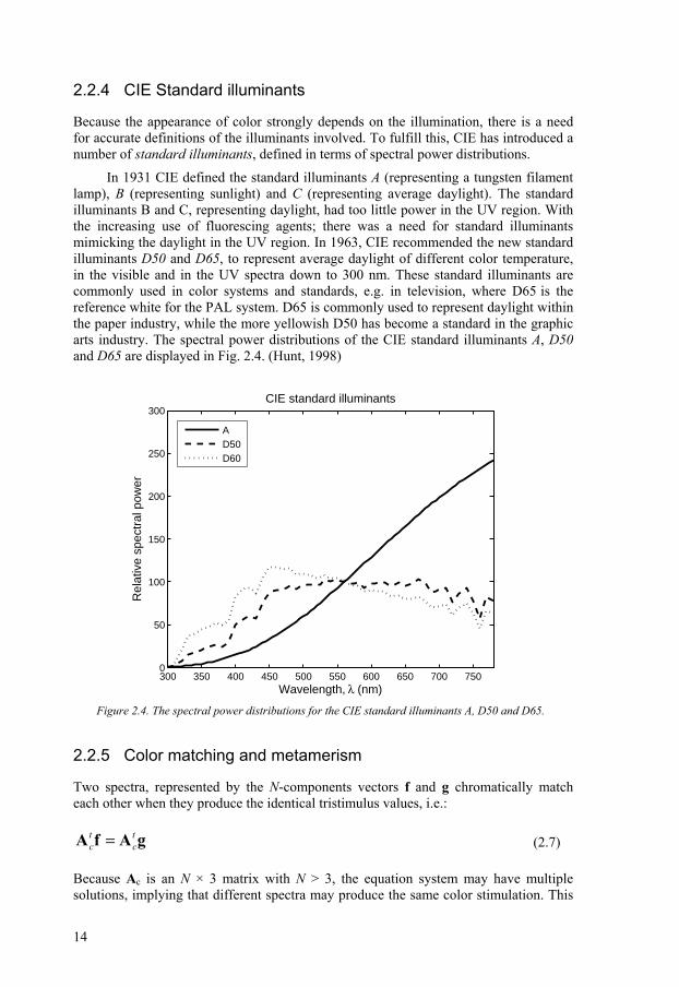
In 1931 CIE defined the standard illuminants A (representing a tungsten filament lamp), B (representing sunlight) and C (representing average daylight). The standard illuminants B and C, representing daylight, had too little power in the UV region. With the increasing use of fluorescing agents; there was a need for standard illuminants mimicking the daylight in the UV region. In 1963, CIE recommended the new standard illuminants D50 and D65, to represent average daylight of different color temperature, in the visible and in the UV spectra down to 300 nm. These standard illuminants are commonly used in color systems and standards, e.g. in television, where D65 is the reference white for the PAL system. D65 is commonly used to represent daylight within the paper industry, while the more yellowish D50 has become a standard in the graphic arts industry. The spectral power distributions of the CIE standard illuminants A, D50 and D65 are displayed in Fig. 2.4. (Hunt, 1998)

Figure 2.4. The spectral power distributions for the CIE standard illuminants A, D50 and D65.

2.2.5 Color matching and metamerism

Two spectra, represented by the N-components vectors f and g chromatically match each other when they produce the identical tristimulus values, i.e.:

t tc c=A f A g (2.7)

Because Ac is an N × 3 matrix with N > 3, the equation system may have multiple solutions, implying that different spectra may produce the same color stimulation. This

300 350 400 450 500 550 600 650 700 7500

50

100

150

200

250

300

Wavelength, λ (nm)

Rel

ativ

e sp

ectr

al p

ower

CIE standard illuminants

AD50D60

15

phenomenon is called metamerism which means that two different spectra result in the same tristimulus values, i.e. appearing having the same color, under a given illumination. The pair of distinct spectra producing the same tristimulus values are called metamers and the match is referred to as a metameric match, as opposed to a spectral match.

One effect of metamerism is that two colors that match under a given illuminant may look very different when they are viewed under another illumination. This causes, sometimes, practical problems, for example when clothes that match perfectly in a dressing room may appear differently in outdoor environment. Besides being problematic sometimes, metamerism is the basis for conventional color reproduction, using three primary colors to achieve a colorimetric match to the target color, rather than a spectral match (Sec. 2.4).

To describe the various types of metamerism, CIE has recommended the use of metamerism indices. The Illuminant Metamerism Index considers the color difference between a metameric pair, caused by substituting a reference illuminant (preferably D65) by a test illuminant. The Observer Metamerism Index measures the color difference between a metameric pair caused by substituting the reference observer (either the 2˚ observer or the 10˚ observer) by a Standard Deviate Observer (SDO), having different spectral sensitivities. (Hunt, 1998)

2.2.6 CIELAB color space

The CIEXYZ tristimulus values provide the basis for colorimetry representing colors in the three-dimensional XYZ color space. It is natural and practically useful to associate the differences in the XYZ color space to the perceived difference. Unfortunately, the visual system is complex and the eyes sensitivity to light is nonlinear, in contrast to the tristimulus values that are linearly related to the spectral power of the light (Eq. 2.3). Therefore, the XYZ color space is perceptually non-uniform, i.e. the Euclidian differences in XYZ color space between colors do not correspond to the perceived color differences.

To linearly map the Euclidian distance in a color space into the perceptual color difference, a perceptually uniform color space is needed. In 1976 CIE proposed the CIE 1976 (L*a*b*) color space, (CIELAB), which is approximately uniform. The CIELAB coordinates are computed using non-linear transformations from the tristimulus XYZ values, as:

13

116 16 0.008856*

903.3 0.008856

n n

n n

Y YY YL

Y YY Y

⎧⎛ ⎞ ⎛ ⎞⎪ − >⎜ ⎟ ⎜ ⎟⎪⎪ ⎝ ⎠ ⎝ ⎠= ⎨

⎪ ⎛ ⎞ ⎛ ⎞≤⎪ ⎜ ⎟ ⎜ ⎟

⎪ ⎝ ⎠ ⎝ ⎠⎩

(2.8)

* 500n n

X Ya f fX Y

⎡ ⎤⎛ ⎞ ⎛ ⎞= −⎢ ⎥⎜ ⎟ ⎜ ⎟

⎢ ⎥⎝ ⎠ ⎝ ⎠⎣ ⎦ (2.9)

16

* 200n n

Y Zb f fY Z

⎡ ⎤⎛ ⎞ ⎛ ⎞= −⎢ ⎥⎜ ⎟ ⎜ ⎟

⎢ ⎥⎝ ⎠ ⎝ ⎠⎣ ⎦ (2.10)

where

13 0.008856

( ) 167.787 0.008856116

x xf x

x x

⎧>⎪

= ⎨⎪ + ≤⎩

(2.11)

The values Xn, Yn and Zn refers to the CIEXYZ tristimulus values of a reference white, usually represented by one of the CIE standard illuminants. The use of the reference white is an attempt to account for the adaptive characteristics of the visual system. The purpose of using a linear model at lower light levels is because the cones become less sensitive while the rods become active at low levels of light (Trussel, et al., 2005).

The CIELAB color space is defined by the three coordinates L*, representing lightness, a*, representing the red-green axis, and b*, representing the yellow-blue axis, see Fig. 2.5. The scale of L* is 0 to 100, with 0 representing black and 100 the reference white. A variant of the CIELAB representation is the cylindrical coordinates, defined by the CIE 1976 chroma,

2 2* ( *) ( *)abC a b= + (2.12) and the CIE 1976 hue-angle,

** arctan*ab

bha

⎛ ⎞= ⎜ ⎟⎝ ⎠

(2.13)

Figure 2.5. Interpretation of the L*, a* and b* axes in CIELAB color space.

17

It is important to point out that the CIELAB color space is only approximately uniform, sometimes referred to as being a pseudo-uniform color space. There are still significant differences in the correspondence to the perceived color differences in the different parts of the CIELAB space, with the blue region being especially problematic (Sharma, 2003). Since there is no ideal uniform color space available, the CIELAB color space probably represents the most important colorimetric system at present (Kipphan, 2001).

2.2.7 Color difference formulae

When comparing colors it is desirable to define a measure for the perceived difference in color appearance. A color difference formula is designed to give a quantitative measure of the perceived color difference between a pair of color samples under a given set of conditions. One simple and commonly used color difference formula is the CIE 1976 L*a*b* color difference, ∆E*ab, corresponding to the Euclidian distance in CIELAB color space, i.e.

2 2 2* ( *) ( *) ( *)abE L a b∆ = ∆ + ∆ + ∆ (2.14) where ∆L*, ∆a* and ∆b* are the differences in L*, a* and b*, respectively, between the pair of samples. An alternative formulation of the CIE 1976 color difference is expressed in terms of the lightness difference, ∆L*, chroma difference, ∆C*ab, and hue difference, ∆H*ab, as:

2 2 2ab ab* ( *) ( * ) ( * )abE L C H∆ = ∆ + ∆ + ∆ (2.15)

Note that the hue difference is not defined as the difference in hue angle, h*ab, but as:

2 2 2ab* ( * ) ( *) ( * )ab abH E L C∆ = ∆ − ∆ − ∆ (2.16)

The perceptual interpretation of the color difference ∆E*ab is not straightforward and there are a number of different interpretations proposed. The just noticeable difference (JND) is about 1 ∆E*ab (Hunt, 1995) but varies for different parts of CIELAB space. A “rule of thumb” for the interpretation of the ∆E*ab color difference is given in Table 2.1 (Hardeberg, 2001):

Table 2.1. Perceptual impact of ∆E*ab color difference between two color samples, in side by side comparison.

∆E*ab Effect

< 3 Hardly perceptible

3 - 6 Perceptible but acceptable

> 6 Not acceptable

18

In a perceptually uniform space, the Euclidian distance would provide a good metric of the perceived color difference. However, the non-uniformities of CIELAB result in variations in the perceptual correspondence to ∆E*ab in different parts of the color space. In 1994, CIE proposed a revised color difference formula, the CIE 1994 color difference, which incorporates corrections for the non-uniformity of CIELAB (CIE, 1995). The CIE94 color difference, ∆E*94, is given by:

22 2

ab ab94

* * **L L C C H H

L C HEk S k S k S

⎛ ⎞⎛ ⎞ ⎛ ⎞∆ ∆ ∆∆ = + +⎜ ⎟⎜ ⎟ ⎜ ⎟⎝ ⎠ ⎝ ⎠⎝ ⎠

(2.17)

where the weighting functions SL, SC and SH vary with the chroma of the reference sample, as:

1, 1 0.045 *, 1 0.015 *L C HS S C S C= = + = + (2.18) The parametric factors kL, kC, kH are included to account for the influence on viewing and illumination conditions. Under reference conditions they are set to:

1L C Hk k k= = = (2.19)

A given color difference, represented by equally sized spheres of ∆E*ab, is in ∆E*94 represented by elliptical volumes, with the size and shape varying throughout the color space. For neutral colors ∆E*94 equals ∆E*ab, while ∆E*94 becomes smaller for more saturated colors.

The latest attempt for improving the uniformity of color difference formula is the CIEDE2000 (Lou, et al., 2000; CIE, 2001). Beside the chroma and hue weighting functions used in CIE94, CIEDE2000 include a number of additional parameters to further compensate for the non-uniformity of CIELAB. However, the improvements achieved by incorporating the more advanced corrections in the formula, are found to be small compared to the improvements of the CIE94 formula (Melgosa, et al., 2004)

2.3 Color measurements

2.3.1 Instruments

Color measurement instruments, fall into two general categories: broadband and narrowband instruments. Broadband instruments uses broadband filters to filter the incoming radiation and delivers up to three color signals. Photometers measure luminance only, densitometers give the optical density for red, green and blue. Colorimeters record CIE tristimulus values directly, by using photocells combined with color filters designed to match the CIE color matching functions. They are fast and relatively inexpensive, but their accuracy is limited because it is difficult to design filters that exactly match the color matching functions. Accurate colorimetric

19

measurements require computation from spectral power data, delivered by narrow band instruments.

Measuring spectral data involves spectroradiometry or spectrophotometry. In spectroradiometry, the incoming radiation is measured in narrow bands of wavelengths throughout the spectrum, using spectroradiometers. In spectrophotometry, the amount of reflected light from an object is compared to the incident light, thus delivering a measure of the spectral reflectance for the sample.

Both spectroradiometers and spectrophotometers require means of dispersing the light into a spectrum, such that light at different wavelengths can be measured. Usually the light is dispersed using gratings, but prisms and narrowband interference filters can also be used. The dispersed radiation is then detected by photoelectric cells. In the case of spectrophotometers, a light source is also required, most commonly tungsten-halogen lamps or xenon flash lamps.

For most purposes, it is considered sufficient to sample the spectrum at 5 nm intervals, but in some cases 10 nm or 20 nm intervals are also appropriate. The CIE color matching functions are tabulated in the range 360 to 830 nm, but for most colorimetric purposes it is considered sufficient to use the range 380 to 780 nm. Some instruments use smaller range of wavelengths, commonly 400 to 700 nm. (Hunt, 1998)

2.3.2 Measurement geometry

An important consideration in color measurements is the geometry of viewing and illumination. CIE has recommended 6 different geometries for colorimetric measurements of reflective samples and another 6 for transmission measurements (Hunt, 1998).

A common arrangement for reflective measurements within the graphic arts industry is the 45°/0° geometry, denoting for 45° angle of incident illumination and with the detector normal to the surface. The geometry is intended to reduce the effect of specular reflection and to represent typical viewing conditions. The disadvantage is that the result is dependent on the structure of the surface topology because of the directed illumination.

The d/0° geometry, denoting for diffuse illumination and measurement from surface normal, is commonly used for color measurements within the paper industry. The diffuse illumination is provided by an integrating sphere whose inside is coated with a highly reflective material, usually barium sulfate. The sample is placed against an opening in the sphere, and the illumination is arranged so that neither the sample nor the detector is directly illuminated, i.e. so that only diffuse illumination strikes the sample, and so that no light from the illuminant directly reaches the detector. (Pauler, 1998)

2.3.3 Precision and accuracy in color measurements

By precision is meant the consistency with which measurements can be made, i.e. the ability to deliver stable and repeatable results. Precision is affected by random errors and the most common sources are variation in sensitivity, electronic noise and sample preparation.

20

By accuracy is meant the degree to which measurements agree to those made by a standard instrument or procedure in which all possible errors are minimized. Accuracy is affected by systematic errors and common sources in modern instruments are wavelength calibration, detector linearity, measurement geometry and polarization.

The importance of precision and accuracy depends on the application. For example, when the same instrument is used to monitor the consistency of a product, good precision is vital, but great accuracy is not. When colorimetric results from different instruments are to be compared, good accuracy is crucial. Furthermore, for any comparison to be meaningful, it is essential that the illuminant, standard observer, and the measurement geometry must all be the same. (Hunt, 1998)

2.4 Color imaging In the real world, colors exist as spatial variation of spectral distributions of radiance and reflectance. To capture these scenes digitally using a color recording device, the images must be sampled, both spatially and spectrally. The captured color images are reproduced from recorded data, typically by using additive or subtractive color mixing of a set of primary colors.

2.4.1 Color image acquisition

Digital color recording devices consist mainly of digital cameras or color scanners, operating on similar principles. The color information is recorded by optical-electronic sensors that spatially sample the image. Light from the image passes through a number of color filters of different spectral transmittance before it reaches the sensors. The transmission filters typically consist of a set of red, green and blue filters, producing RGB-images.

The sensors in digital cameras are typically arranged as two-dimensional arrays, allowing for the image to be captured in a single exposure. There exist different schemes for separating the RGB color-channels. The most common scheme is color filter arrays (CFAs), where each cell of the sensor is covered with a transmissive filter of one of the primary colors. The most commonly used mosaic pattern for the filters is the Bayer pattern, with 50% green cells in a checker board arrangement, and alternating lines of red and blue cells. Other methods for color separation include color sequential, where the image is composed of sequential exposures while switching the filters, and multi-sensor color, where the light is separated into red, green and blue colors using a beam splitter and detected by three separate monochrome sensors. (Paraluski &. Spoulding, 2003)

Scanners are typically designed to scan images on paper or transparencies using its in-built light source. There is no need to capture the stationary object in a single exposure and typically linear sensor arrays are used to scan the image, moving along the direction perpendicular to the sensor array. Usually three (linear) sensor arrays are used, corresponding to the three color channels, R, G and B, but there is also solutions using three different lamps, obtaining the color image from three successive measurements with a single array. (Sharma, 2003)

21

2.4.2 Color reproduction

Generally speaking, all the color reproduction techniques can be classified into two groups: additive and subtractive. In additive color reproduction, color is produced as an additive mixture of light of different wavelengths, known as primary colors. Typically, the additive primaries are red, green and blue (RGB). The principle of additive color mixture is illustrated in Fig. 2.6(a), where mixing red with green light produces yellow, similarly, red and blue produces magenta, blue and green forms cyan and the mixture of all three primaries gives white. Additive color reproduction is typically used for emissive displays, such as CRT and LCD displays.

Subtractive color reproduction, typically used for transparent or transmissive media, produces colors by blocking/removing spectral components from “white” light through light absorption. The most common subtractive primaries are cyan, magenta and yellow (CMY), colorants that absorb light in the red, green and blue spectral bands of the spectrum, respectively. The principle is illustrated in Fig. 2.6(b), where the overlay of cyan and magenta producing blue, cyan and yellow produces green, magenta and yellow produces red and the overlay of all three colorants results in black. It is common to add a fourth black (K) colorant, to improve the reproduction of gray tones and allowing for darker colors to be reproduced. (Sharma, 2003)

Figure 2.6. The principle of additive (a) and subtractive (b) color mixing.

2.4.3 Color management

The principles of color image acquisition and reproduction described in the previous sections rely on device-dependent color representations, specific for each device. For example, the RGB primaries of a digital camera or a flatbed scanner are generally different to those of a CRT or a LCD display. In other words, a color image will look differently when displayed on different devices. To achieve consistent color representations with different devices, it is necessary to map the device-dependent color representations into a device-independent space, which is the key of color management.

In digital color management, the device-independent color space is called the profile connection space (PCS). CIEXYZ and CIELAB are the commonly used profile connection spaces. The transformations between device-dependent data and the PCS are

22

described by device profiles, for input and output devices. The device profiles, defining the relationship between device-dependent and device-independent color spaces are derived by device characterization, as described in Chapter 3. A widely adopted standard for storing device profiles is the International Color Consortium (ICC) profile (ICC, 2004). A color management module (CMM) is responsible for interpreting the device profiles and performing the transformation to and from the device-independent profile connection space. The principle of ICC color management is illustrated in Fig. 2.7.

Figure 2.7. The ICC color management system. The relationship between device colors and the profile connection space (PCS) are described by ICC-profiles, for input and output devices.

Ideally, the color management system should perform accurate color transformations between different types of media and devices, but to achieve this is not a trivial task. First, there are significant differences in the gamuts of reproducible colors for different color devices. Furthermore, the differences in viewing conditions for different media imply that a simple colorimetric match does not necessarily give an appearance match. (Sharma, 2003)

2.5 Multispectral imaging

2.5.1 Background

The trichromatic nature of human vision was first proposed by Herman Gunther Grassman in 1853, and has later been verified by studies of the human eye. This three-dimensionality of color has formed the basis for colorimetry and for color imaging using three channels, including e.g. modern television, computer displays, as well as film-based photography and digital photography (Fairchild et al., 2001). However, three-channel color imaging has several limitations in color image acquisition and reproduction.

Profile Connection

Space

Scanner

Digital camera

LCD display

Ink-jet printer

Offset printing press

ICC-profile

ICC-profile

ICC-profile

ICC-profile

ICC

-pro

file

23

Three-channel imaging is by its nature always metameric, i.e. based on metameric matching rather than spectral matching. However, the sensitivities of typical imaging devices differ from the CIE color matching functions, thus produces metameric matches that differs from those of a human observer. As an example, consider the ICC workflow, relating device values to colorimetric values, as described in Sec. 2.4.3. When two non-identical spectra are metameric for the input device, they will always map to the same colorimetric values, even though they are not metameric with respect to a human observer. Conversely, when two colors are metameric to an observer but not to the input device, the CMM will in error treat the two as having different colorimetric values. (Rosen, et al., 2000)

The limitations of metameric imaging are further expanded when the effects of illumination are considered. For example, it is possible for a metameric imaging system to be unable to distinguish a white object under a red light from a red object under a white light. (Fairchild et al., 2001). With these limitations in mind, to represent color by its spectral power distributions i.e. multispectral imaging is of clear advantage.

2.5.2 Terminology

The terminology and definitions referring the concepts of multispectral imaging and multi-channel imaging are sometimes confusing, with different meanings by different authors. Throughout this thesis, we will refer to multi-channel images as images containing more then the conventional three color channels (with the exception of CMYK, which is not multi-channel). By multispectral images we mean images in which each pixel contains information about the spectral properties of the samples being imaged. Even though multispectral images are typically derived using multi-channel systems, they can also be derived using conventional trichromatic images (see for example Connah, et al., 2001; Imai & Berns, 1999). Another terminology referring to multispectral imaging is sometimes called multi-channel visible spectrum imaging (MVSI), or simply spectral imaging (Imai, et al., 2002).

2.5.3 The spectral approach

It is well known that the only way to assure a color match for all observers across changes of illumination is to achieve a spectral match (Imai & Berns, 1999). By representing color as spectral power distributions, metamerism in color imaging can be avoided. Further more, it allows for the separation of the spectral properties for the object from the illumination, thus representing the color of an object by its spectral reflectance. As the physical representation of color, spectral reflectance is completely independent of the characteristics of the image acquisition system. Therefore, the differences between any spectra will be distinguished, independently if they are metameric with respect to any illumination, observer or image capturing device. The multispectral images can be transformed to any color space and be rendered under any illumination. Further more, the gamut will not be limited by the set of primaries of a specific imaging device. The concept of multispectral imaging involves capturing, processing and reproducing images with a high number of spectral channels.

The acquisition of multispectral images involves recovering spectral properties of the sample being imaged. Typically, the image is captured using multi-channel systems of narrowband characteristics, but trichromatic systems are also used. Hence,

24

multispectral imaging requires for the computation of spectral reflectance data, from a relatively small number of channels. It is possible simply because the spectral properties of most surfaces are smooth functions of wavelength (Cheung, et al., 2005).

On the reproduction side, spectral imaging systems are capable of producing images that are robust to changing illuminations. If a printer has a large set of inks to choose from, it should be possible to select a subset of inks that achieve a spectral match to the multispectral images (Imai & Berns, 1999). When a printed image have the same reflectance properties as the original object, the original and the reproduction will match under any illumination and for any observer or imaging device (Fairchild, 2001).

2.5.4 Previous work

The interest for multispectral imaging is rapidly increasing and researches are ongoing in several laboratories around the world, focusing on the acquisition, processing and reproduction of multispectral images. For more general descriptions on the concept of multispectral imaging, including aspects on the workflow and processing of the data, we refer to: Berns, et al. (1998), Rosen et al. (2000), Fairchild, et al. (2001), Rosen et al. (2001) and Willert, et al. (2006).

Works that are more specifically directed to the acquisition of multispectral images, the main focus of this thesis, include: Imai & Berns (1999), Sugiura, et al. (1999), Imai et al. (2000), Haneishi, et al. (2000), Hardeberg (2001) and Connah, et al. (2001).

For multispectral approaches to color reproduction, a topic that will not be treated further in this work, refer for example to: Berns, et al. (1998), Tzeng & Berns (2000), Imai, et al. (2001b) and Kraushaar & Urban (2006) for multispectral printing, and to: Ajito, et al. (2000), Yamaguchi, et al. (2001) and Nyström (2002), for multiprimary displays.

25

Chapter 3 3 Device characterization

Device characterization

3.1 Introduction 3.2 Calibration and characterization 3.3 Characterization approaches 3.4 Input devices 3.5 Output devices 3.6 Least-squares regression

techniques 3.7 Metrics for evaluating device

characterization 3.8 Color target design

26

27

3.1 Introduction Device characterization is the process of deriving the relationship between device-dependent and device-independent color representations, for a color imaging device. This chapter intends to provide a background of the concept of device characterization, as well as providing the definitions and terminology associated with the topic.

The difference between device calibration and device characterization is defined, and so is the concept of forward and inverse characterization. The two conceptually different approaches for device characterization, model-based and empirical characterization, are described for input and output devices. Even though the focus of this thesis is characterization of input devices, characterization of output devices have been included for completeness.

Among the different mathematical techniques used for data fitting or data interpolation in device characterization, the focus is on the least squares regression techniques. This intends to provide readers with the theoretical background for the work described in following chapters of the thesis.

3.2 Calibration and characterization It is necessary to distinguish device calibration from device characterization. Device calibration is the process of maintaining a device with a fixed known characteristic color response, and should be carried out prior to device characterization. Calibration may involve simply ensuring that the controls of a device are kept at fixed nominal settings, but it may also include linearization of the individual color channels or gray-balancing.

Device characterization derives the relationship between device-dependent and device-independent color data, for a calibrated device. For input devices, the signal captured by the input device is first processed through a calibration function while output devices are addressed through a final calibration function, see Fig. 3.1. Typically, device characterization is carried out relatively infrequently compared to calibration, which is done more frequently to compensate temporal changes and maintain a device in a fixed known state. The two form a pair, so if the characteristic color response of the

28

device is altered by a new calibration, the characterization should be re-derived. (Bala, 2003)

Figure 3.1. Calibration and characterization for input and output devices. (© Bala, 2003)

The characterization function can be defined in two directions. The forward characterization function defines the response of a device to a known input, thus describing the color characteristics of the device. For input devices, this corresponds to the mapping from a device-independent color stimulus to the device-dependent signals recorded when exposed to that stimulus. For output devices it corresponds to the mapping from the input device-dependent color to the resulting rendered color, in device-independent coordinates. The inverse characterization function compensates for the device characteristics and determines the input that is required to obtain a desired response.

The output of the calibration and characterization processes is a set of mappings between device-independent and device-dependent color data. These can be implemented as some combination of power-law mapping, matrix conversion, white-point normalization and look-up tables. The widely adopted standard to store this information is the ICC (International Color Consortium) profile, used in color management (ICC, 2004).

3.3 Characterization approaches There are generally two different approaches to derive the characterization function: model-based and empirical characterization. For input devices, the two approaches are sometimes referred to as spectral sensitivity based and color target based (Hong & Lou, 2000) or spectral models and analytical models (Hardeberg, 2001).

Model-based characterization uses a physical model that describes the process by which the device captures or renders color. Access to raw device data is generally required, and the quality of the characterization is dependent on how well the model

29

reflects the real behavior of the device. Model-based approaches have better generality and can provide insights into device characteristics.

In empirical characterization, the mapping is made using a black box approach, i.e. without explicitly modeling the device characteristics. By correlating the device response for a number of test colors to the corresponding device-independent values, the characterization function is derived using mathematical fitting. Empirical approaches often provide more accurate characterizations for end-user applications, but the functions derived will be optimized only for a specific set of conditions, including the illuminant, the media and the colorant. Hybrid techniques, which combine strengths from both model-based and empirical approaches, also exist. (Bala, 2003)

3.4 Input devices The two main types of digital color input devices are scanners and digital cameras, recording the incoming radiation through a set of color filters (typically RGB). The calibration of input devices typically involves establishing all settings, such as aperture, exposure time and internal settings, and to determine the relationship between the input radiance and the device response. The main difference between the characterization of scanners and digital cameras is that scanners employ a fixed illumination as part of the system, while digital cameras may capture images under varying and uncontrolled conditions.

3.4.1 Model-based input device characterization

The basic model that describes the response of an image capture device with m color filters is given by:

( ) ( )k k kV

d E S dλ

λ λ λ ε∈

= +∫ (3.1)

where k = 1,…,m (m = 3 for RGB devices), dk is the sensor response, E(λ) is the input spectral radiance, Sk(λ) is the spectral sensitivity of the k:th sensor, εk is the measurement noise for channel k, and V is the spectral sensitivity domain of the device.

If we represent the spectral signal as the discrete N-component vector, f, uniformly sampled at wavelengths λ1,…, λN, Eq. 3.1 can be rewritten as:

td ε= +d A f (3.2)

where d is a m-component vector of device signals (e.g. [R,G,B]), f is the N-component vector of the input spectral signal, Ad is the N × M matrix with columns representing the sensor responses and ε is the measurement noise term. Note that if the wavelength sample interval is larger than l nm, then Eq. 3.2 should be completed with the ∆λ factor.

According to Sec. 2.2, we know that colorimetric signals can be computed by:

tc=c A f (3.3)

30

where c is the colorimetric vector [X,Y,Z] and Ac the N × 3 matrix with columns representing the XYZ color-matching functions.

From Eq.s 3.2 and 3.3, it can be seen that, in the absence of noise, there exist a unique mapping between device-dependent signals d and device independent signals c, when there exist an unique transformation from Ad to Ac. In the case of three channel devices (RGB), the sensor’s response Ad must be a non-singular transformation of the color matching functions, Ac. Devices that fulfill this so-called Luther-Ives condition are referred to as colorimetric devices (Bala, 2001).

Unfortunately, practical considerations make it difficult to design sensors that meet this criterion. The assumption of a noise-free system is unrealistic and most filter sets are designed to have more narrow-band characteristics than the color matching functions, to improve efficiency. For the majority of input devices that do not fulfill the conditions for being colorimetric devices, the relationship between XYZ and device RGB is typically more complex than a linear 3 × 3 matrix. The most accurate characterization is usually a non-linear function that varies with the input medium. (Bala, 2003)

3.4.2 Empirical input device characterization

The workflow for empirical input device characterization is illustrated in Fig. 3.2. After the device has been calibrated, the characterization is performed using a target of color patches that spans the color gamut of the device. The device-dependent coordinates {di} (e.g. RGB) is extracted for each color patch and correlated with the corresponding device-independent values {ci} (typically XYZ or L*a*b*), obtained using a spectroradiometer or spectrophotometer.

Figure 3.2. A schematic diagram for the workflow of empirical input device characterization. (© Bala, 2003)

3.5 Output devices Recall from Chapter 2 that output color devices can be usually categorized into two groups: emissive devices producing colors via an additive mixing of red, green and blue (RGB) lights, and devices that produces reflective prints or transparencies via subtractive color mixing.

31

3.5.1 Model-based output device characterization

In the case of emissive displays, the characterization is greatly simplified by the assumptions of channel independence and chromaticity constancy. This mean that each of the RGB channels operates independently of the other and that the spectral radiance from a given channel has the same basic shape and is only scaled as a function of the signal driving the display. With these assumptions, model-based display characterization is a fairly simple process, resulting in a 3 × 3 matrix conversion relating XYZ to RGB.

The calibration of emissive displays involves finding the relation between the RGB input values and the resulting displayed luminance. This relationship is typically modeled using a power-law relationship (gamma correction) for CRT-displays, while LCD-displays are better modeled using a sigmoidal S-shaped function

The output devices based on subtractive color mixing exhibit complex nonlinear color characteristics, which makes model-based approach a challenge. The spectral characteristics of process inks do not fulfill the ideal “block dye” assumption and the halftoning introduces additional optical and spatial interactions, and thus further complexity. Nevertheless, much effort has been devoted to modeling color reproduction of printing. Examples of physical models, describing the forward characterization, include the well known Neugebauer, Yule-Nielsen and Kubelka-Munk models (see for example Emmel, 2003).

3.5.2 Empirical output device characterization

The workflow for output device calibration and characterization is illustrated in Fig. 3.3. A digital target of color patches with known device values (e.g. RGB or CMYK) is sent to the device and the resulting (displayed or printed) colors are measured in device-independent coordinates. A relationship is established between device-dependent and device-independent color representations, which can be used to derive the characterization function. To evaluate the calibration and characterization, independent test targets should be used.

Figure 3. 3. The workflow for Empirical output device characterization. (© Bala, 2003)

32

3.6 Least-squares regression techniques In empirical approaches, the characterization function is derived by relating the device response, di, to the corresponding device-independent values, ci, for a set of color samples. In the following, let {di} be the m-dimensional device-dependent coordinates for a set of T color samples, and {ci} be the corresponding set of n-dimensional device-independent coordinates (i = 1,…,T). For most characterization functions, n = 3 (typically. XYZ or L*a*b*) and m = 3 or 4 (typically RGB or CMYK). Note however, that for multi-channel imaging systems m >3, depending on the number of color channels utilized. The pair ({di},{ci}) refers to the set of training samples and is used to evaluate one or both of the following functions:

nm RRf →∈F: , mapping the device-dependent data with the domain F to device independent color space.

mn RRg →∈G: , mapping device-independent data with the domain G to device-dependent color space.

To derive the characterization functions, mathematical techniques as for instance, data fitting or interpolation are used. A common approach is to parameterize f (or g) and to find the parameters by minimizing the mean squared error metric, using least-squares regression.

Other approaches for data fitting and interpolation in device characterization include, for example, lattice-based interpolation, spline fitting and the use of neural networks. (Bala, 2003)

3.6.1 Linear least squares regression

The simplest form of least squares regression is linear least squares regression. The characterization function is approximated by a linear relationship c = d · A, where d is the 1 × m input color vector and c is the 1 × n output color vector.

The optimal m × n matrix A is derived by minimizing the mean squared error of the linear fit to the set of training samples ({di},{ci}), as:

⎪⎭

⎪⎬⎫

⎪⎩

⎪⎨⎧

−= ∑=

2

1

1minargT

iii

Aopt T

AdcA (3.3)

If the samples {ci} are collected into a T × n matrix C = [c1, …,cT] and {di} into a T × m matrix D = [d1, …,dT], then the linear relationship is given by : C = DA (3.4) and the optimal A is given by:

CDCDDDA −− == )()( 1 tt (3.5)

33

where (D)- = (DtD)-1Dt denotes for the Moore-Penrose pseudo-inverse of D, which sometimes refers to the generalized inverse.

3.6.2 Polynomial regression

Polynomial regression is a special case of least squares regression, where the characterization function is approximated by a polynomial. For example, the inverse characterization function of a 3-channel system, mapping RGB values to XYZ tristimulus values, is obtained by expressing XYZ as a polynomial function of R, G and B. The regression from 3ℜ to 3ℜ , i.e. from RGB to XYZ, is equivalent to three independent regressions from 3ℜ toℜ , i.e. from RGB to each of the XYZ components (Hardeberg, 2001). As an example, the second order polynomial approximation is given by:

[ ],1 ,1 ,1

,2 ,2 ,22 2 2

,10 ,10 ,10

1, , , , , , , , ,...

X Y Z

X Y Z

X Y Z

w w ww w w

X Y Z R G B R RG RB G GB B

w w w

⎡ ⎤⎢ ⎥⎢ ⎥⎡ ⎤= ⎣ ⎦ ⎢ ⎥⎢ ⎥⎣ ⎦

(3.6)

or, generally:

=c pA (3.7) where c is the n-component colorimetric output vector, p is the Q-component vector of polynomial terms derived from the input vector d, and A is the Q × n matrix of polynomial weights to be optimized.

After arranging the input device data d into the polynomial vector p, the polynomial regression is reduced into a linear least squares regression problem, with the optimal matrix of polynomial weights, A, given by:

⎪⎭

⎪⎬⎫

⎪⎩

⎪⎨⎧

−= ∑=

2

1

1minargT

iii

Aopt T

ApcA (3.8)

Again, collecting the samples {ci} into a T × n matrix C = [c1, …,cT] and the polynomial terms {pi} into a T × Q matrix P = [p1, …,pT], the relationship given in Eq. 3.7 can be rewritten as:

=C PA (3.9) Then, the optimal solution for A is given by:

1( ) ( )t t− −= =A P P P C P C (3.10)

34

where (P)- denotes for the pseudo-inverse of P. In order that the Q × Q matrix (Pt P) to be invertible, it requires for T ≥ Q, i.e. the number of the training colors should be as many as the number of polynomial terms. For the preferred case, T > Q, we have an over determined system of equations for which we derive the least-squares solution. Unfortunately, the number of the polynomial terms increases rapidly with the order of the polynomial. For a third-order polynomial, for example, in the complete form including all the cross-product terms, there is Q=64. Therefore, simplified approximations are commonly used, with a smaller number of polynomial terms than in the complete form. In general it is recommended to use the smallest number of polynomial terms that adequately fits the function while still smoothening out the noise. (Bala, 2003)

3.7 Metrics for evaluating device characterization Generally speaking, the minimized quantitative error metrics of the regression provide an indicator of the overall accuracy of the characterization. However, in the current application, using the regression error alone is not sufficient to evaluate the characterization, for several reasons. First, the error is available only for the training samples used to derive the characterization function. Hence the accuracy of the characterization should be evaluated using independent test targets, not the training colors. Furthermore, the error used in the fitting or interpolation techniques, is not always calculated in a visually meaningful color space. Evaluation of errors should preferably be within visually relevant metrics, such as the color difference formulae ∆E*ab or ∆E*94, previously described in Sec. 2.2.

The statistics usually reported in literature, when evaluating device characterization, are the mean, maximum and standard deviation, of the ∆E values for a set of test samples. The 95th percentile of ∆E values (i.e. the value below which 95% of the ∆E values lie) is also often computed. To judge whether the characterization error is satisfactory small or not, using the chosen error metric, depends very strongly on the application and the expectations from the user. The accuracy of the characterization will also be limited by the inherent stability and uniformity of a given device. (Bala, 2003)

3.8 Color target design The first factor to consider in color target design is the set of colorants and underlying medium of the target. For input devices, where the target is not created as part of the characterization process, the colorants and media should be representative of what is likely to be used for the device. For output color devices, the generation of the target is part of the characterization process, and should be carried out using the same colorants and media as in the final color rendition.

Another factor is the choice of color patches. Typically, they are chosen to span the desired range of colors to be captured (input devices) or rendered (output devices). Considering the spatial layout of the patches, it may be desirable to generate targets with the same colors in different spatial layouts. In such a manner, measurements from multiple targets can be averaged, to reduce the effects of non-uniformity and noise in the characterization process. (Bala, 2003)

35

A few targets have been adopted as industry standards, e.g. the GretagMacbeth ColorChecker chart and the Kodak photographic Q60 target for input device characterization, and the IT8.7/3 CMYK target for printer characterization.

36

37

Chapter 4 4 Calibration of the image acquisition system

Calibration of the image acquisition system

4.1 Introduction 4.2 The Image acquisition system 4.3 Illumination 4.4 Color filters 4.5 Optics 4.6 CCD camera 4.7 Summary and discussion

38

39

4.1 Introduction To obtain repeatable and reliable image data of high quality, it is necessary to know the characteristics of all the components involved in the image acquisition process. This chapter focuses on the calibration of the image acquisition system, with the aim to ensure stable and repeatable results.

For all the components in the system, the technical specifications are given, along with some general background and a discussion on the demands placed on each component for high quality image acquisition. Recommendations for settings and calibration routines are given, based on measurement results and on the demands and properties for each component. The calibration has resulted in so much information that can not be included in a single chapter. The rest are therefore put into the appendix. People who are interested in the details can continue to read Appendix A.

The emphasis in this chapter lies on obtaining device-dependent data in a repeatable and stable way, commonly referred to as obtaining precision in color measurements. It will form the necessary base for the following chapters, focusing on methods on how to transform the acquired device-dependent data into device-independent color representations of high accuracy.

4.2 The Image acquisition system The image acquisition system is an experimental system with great flexibility for the user and numerous ways to control and alter the image acquisition setup. While possible to capture images of arbitrary objects, the primary usage is to capture macro images of flat objects, such as substrates.

4.2.1 Image acquisition setup

The substrate is placed on a table which allows for motor-driven translation in x-y directions and rotation around the optical axis. The illumination is provided using a tungsten halogen lamp through optical fibers, which offers directed light with an adjustable angle of incidence for reflectance images. By using a backlight setup, imaging with transmitting illumination is also possible. The images are captured using a

40

monochrome CCD camera combined with macro optics, consisting of enlarging lenses and various extension rings.

Color images are captured sequentially, using filters mounted in a filter wheel in the optical path. By using this color sequential method, full color information is acquired in every single pixel and there is no need for any interpolation or de-mosaicing, as is the case for conventional digital cameras using color filter arrays. The filter wheel contains 20 color filters, including RGB-filters, CMY-filters and a set of neutral density filters of various optical densities. Furthermore, a set of 7 interference filters allow for the acquisition of multi-channel images. All the components of the image acquisition system are controlled using a Matlab interface. Figure 4.1 illustrates the image acquisition setup, in the mode of reflective imaging.

Figure 4.1. The image acquisition setup for reflectance imaging.

4.2.2 Spectral model

The linear model describing the image acquisition process, in the case of reflectance imaging, is given in Eq. 4.1. The device response, dk, for the k:th channel is, for each pixel, given by:

( ) ( ) ( ) ( ) ( )k k kV

d I F R O QE dλ

λ λ λ λ λ λ ε∈

= +∫ (4.1)

where I(λ) is the spectral irradiance of the illumination (including the spectral characteristics of lamp as well as the optical fibers used for light transportation), Fk(λ) is the spectral transmittance of filter k, R(λ) is the spectral reflectance of the object, O(λ) is the spectral transmittance of the optics, QE(λ) is the spectral quantum efficiency for the CCD sensor, ε k is the measurement noise for channel k, and V is the spectral sensitivity region of the CCD sensor.

When the illumination backlight setup is used to measure object transmittance, T(λ), the spectral transmittance properties of the transmissive plate on which the sample is placed, Tp(λ), must also be included in the model, as:

Fk(λ)

O(λ) QE(λ) R(λ)

I(λ)

Ek(λ) dk

S(λ)

41

( ) ( ) ( ) ( ) ( ) ( )k k kV

d I F T Tp O QE dλ

λ λ λ λ λ λ λ ε∈

= +∫ (4.2)

If any additional filter, e.g. a polarization filter, is used, obviously their spectral characteristics must also be included in the image acquisition system model.

The amplitude of the camera response value, dk, will also depend on the aperture size, the exposure time, and on the focal length used. However, this will only affect the total level of incoming radiance to the CCD sensor, i.e. it is not wavelength dependent, and need not to be included into the spectral model of the camera response.

4.2.3 Spectral measurements

The spectral characterization of the illuminant and the color filters is straight forward, since it can be can be obtained by direct measurements. Spectral measurements are performed using the spectroradiometer PR-650 SpectraScan from Photo research. The spectrophotometer is mounted using a special holder, placing it in the same optical axis as the CCD camera. The spectral data obtained are in the interval 380 to 780 nm sampled at 4 nm intervals (Photo Research, 1999).

Except for the measurements on the transmissive plate, all measurements are performed against a diffuse white reflectance standard, using the 45°/0° measurement geometry. The reflectance standard gives 99% reflectance ± 1% over the photopic region, and is placed in a special holder placing it in the same image plane as the object, to share the same illumination characteristics.

4.3 Illumination The illumination plays a very important role in an image acquisition system and needs to fulfill the following requirements (Hardeberg, 2001):

The geometry should ensure a good spatial uniformity over the scan area, or otherwise be corrected for. If the camera is to be used for spectrophotometric or colorimetric measurements, a lighting/viewing geometry recommended by the CIE should be used (typically 45°/0° geometry).

The power of the lamp should be high enough to give a sufficient signal even through the most narrow-band filters used in the system. Using longer exposure times can compensate for low intensity, but could pose additional problems, such as slower acquisitions and amplified noise.

The spectral properties of the lamp should ensure that there is sufficient power in the whole visible spectrum. Furthermore, it is desirable to use lamps with a smooth spectral power distribution without any sharp peaks.

Stability and repeatability of the irradiance from the light source is of great importance for reliable and accurate measuring results.

42

4.3.1 The Illumination set-up

The illumination is provided by a tungsten halogen lamp through optical fibers. The lamp has been equipped with an infrared (IR) cut-of filter, to block non visible IR radiation. After passing through the color filters in the filter wheel, the light is led by the fibers in one of the two possible directions; to provide either backlight for transmission images, or directed light from above, for reflection images. When the backlight setup is used, the light passes through a transmissive plate, which scatters the light to give a diffused and uniform illumination over the image area. For reflection measurements, the angle of incidence can be controlled from 10º to 80º. The default angle is 45º which, along with the camera normal to the image plan, provides the standard lighting/viewing geometry 45°/0°, as recommended by CIE.

4.3.2 The lamp

The light source used in the image acquisition system consists of a 150W tungsten halogen lamp from Schott-Fostec. The lamp ‘DCR III’ runs on direct current with a regulated voltage supply adjustable from 0.5 to 20.5 VDC, remotely controlled via the Matlab interface. The specific lamp type used, ‘DDL’, has a nominated rated lifetime of 500 hours at 3150K color temperature, when operated at full lamp intensity. When operated at lower intensity, the lifetime increases, while the color temperature decreases. (Schott-Fostech, 2002)

Generally, tungsten halogen lamps can run at higher color temperature, and with better efficacy, than ordinary lamps. The envelope is made of pure fused silica (‘quartz’); it is smaller than ordinary lamps and therefore runs at a much higher temperature. The envelope contains halogen gas. When tungsten evaporates it forms tungsten halide, a gas that migrates back to the filament in a continuous cycle. Therefore, the dark deposits on the envelope can be avoided. (Hunt, 1998)

4.3.3 Recommended lamp intensity

The spectral properties of the lamp are strongly dependent on the intensity level it is operated at. For the lower lamp intensity levels, the color temperature decreases dramatically and the irradiance from the lamp contains almost no power in the blue band of the spectrum. Furthermore, the relation between the radiant power is not linear with respect to lamp intensity level. For example, a lamp intensity level of 50% generates only 15% of the radiant power compared to full intensity level (see Appendix A, for details).

At which lamp intensity level to operate the lamp must be a trade-off between the contradictory demands of increasing the lifetime, considering the cost of replacement lamps and possible degradation effects for an aging lamp, and providing sufficient radiant power throughout the visible spectrum. Taking these into consideration, we recommend that the lamp should be operated at 90% intensity level. The spectral power at 90% intensity level is very close to that of 100% while the nominal lamp lifetime is prolonged for about 80% compared to full intensity, i.e. 900 hours lifetime instead of 500. In the following, all calibration and characterization will be based upon the recommended 90% intensity level.

43

4.3.4 Stability and repeatability

According to the manufacturer, the output voltage of the power supply stabilizes immediately, while a cold lamp takes typically 25 minutes to stabilize within 1% or better. This stabilization period is only slightly affected by the lamp voltage used. Measurements verify that this promise holds, but at the same time indicate that 25 minutes warm-up time may not always be sufficient, when the highest precision is required.

Figure 4.2 displays camera response values during the warm-up cycle for the lamp over a period of 120 min. The measurements have been repeated at 4 different occasions, each time starting with a cold lamp. Clearly, the most dramatic changes occur during the very first minutes, with up to 5% decrease in power. After 25 minutes, the difference between the measurements is still over 0.5% and the power continues to decrease with up to an additional 0.8% during the following hour. Notice that the lamp stabilization cycle differs between the different measurements, with the consequence that repeatability between measurements is hard to attain before the lamp is sufficiently warmed-up and stable.

Figure 4.2. Mean camera response values during the warm up time for the lamp. Measured at 4 different occasions, starting with a cold lamp.

The warm-up time required depends on the demands on accuracy of imaging. For highest accuracy, the warm-up time should be extended to 60, or preferably, 90 minutes. After 60 minutes the maximum difference between the measurements is 0.25% and after 90 minutes it is down to 0.1%. From this point, the lamp can be considered as fairly stable, with only small changes during the following hours. Measurements over longer periods of time have revealed that the power continues to decrease, but in a much slower pace. The change in lamp intensity after the first 90 minutes of burning time, and over the following 10 hours, is in the order of magnitude 0.1%.

0 20 40 60 80 100 1200.9

0.91

0.92

0.93

0.94

0.95

0.96

0.97Lamp warm−up time

Time (min)

Nor

mal

ized

cam

era

resp

nse

44

4.3.5 Uniform illumination

To obtain spatial uniformity in the images acquired, the illumination should be uniform over the entire scan area, or any non-uniformity should otherwise be compensated for. Considering the small field of view, due to the large magnification of the optics, uniform illumination over the scan area should not be hard to achieve. However, for shorter focal lengths giving a larger field of view, non-uniform illumination was detected, due to the directed properties of the light and the rather small light cone. This was encountered for by reconstructing the holder for the optical fibers, increasing the distance to the image plane and yielding a larger light cone area.

Descriptions on how to correct/compensate for non uniform illumination are given in Sec. 4.6, together with corrections for dark current and CCD gain offset.

4.3.6 Spectral properties

Figure 4.3 displays the normalized spectral distribution of the illumination system, including the lamp and the optical fibers, measured against the white reflectance standard, using a warmed up lamp at 90% intensity. The spectral distribution is relatively smooth, without sharp peaks. The spectral power decreases in the blue domain of the spectrum and is low in spectral band below 400 nm. Due to the IR cut-off filter, the spectral power is very low in the band above 750 nm. To block out IR radiation is important, since the CCD sensor is sensitive even in the IR-band, which is a common source of errors, when non-visible light affects the camera response (Hardeberg, 2001; Bala, 2003).

The spectral transmittance of the transmissive plate, which should be included in computations from transmission images, is given in the Appendix.

Figure 4.3. Spectral power distribution for the illumination at 90% lamp intensity level.

400 450 500 550 600 650 700 7500

0.1

0.2

0.3

0.4

0.5

0.6

0.7

0.8

0.9

1Illumination

Wavelength, λ (nm)

Rel

ativ

e sp

ectr

al p

ower

45

4.4 Color filters The filter wheel in the image acquisition system offers the possibility of using up to 20 different filters in the optical path of the light source. Any filter with the standard diameter 25 mm can be set into the filter wheel, and the filters can easily be replaced by the user for different purposes. The standard set of filters used in the filter wheel, consists of 2 sets of RGB and CMY filters, a set of 7 broadband interference filters, and a set of 6 neutral density (ND) filters of various optical densities. The first position is empty, allowing for measurement without any filter, i.e. I(λ) directly.

The spectral transmittance for all filters in the filter wheel has been measured. For each channel, k, the spectral irradiance Ek(λ) is measured against the reflectance standard, and the filter transmission Fk(λ) is given by:

( ) ( ) / ( )k kF E Iλ λ λ= (4.3)

4.4.1 RGB- and CMY-filters

The sets of RGB and CMY filters consist of high saturation dichroic glass filters. The spectral transmittance for the red, green and blue filters, used for RGB-images are displayed in Fig. 4.4. The spectral transmittance for cyan, magenta and yellow (CMY) filters, are displayed in Fig. 4.5.

Figure 4.4. Spectral transmittance for the RGB-filters.

400 450 500 550 600 650 700 7500

0.1

0.2

0.3

0.4

0.5

0.6

0.7

0.8

0.9

1

Wavelength, λ (nm)

Filt

er tr

ansm

ittan

ce

Filter transmittance: RGB−filters

RGB

46

Figure 4.5. Spectral transmittance for the CMY-filters.

4.4.2 Interference filters

The filters used for multi-channel image acquisition are 7 broadband interference filters with their center wavelengths (CWL) at 400 nm, 450 nm, 500 nm, 550 nm, 600 nm, 650 nm and 700 nm, respectively. All the interference filters have a bandwidth of 80 nm full width-half maximum (FWHM), except for the filter with 400 nm CWL, having 50 nm FWHM. The center wavelength tolerance is ±15nm and the peak transmittance ranges from 55% to 60%, according to manufacturer’s specification. Note that the center wavelength corresponds to the midpoint of the pass-band specified by the FWHM which, for interference filters, is normally different from the peak transmittance wavelength. The spectral transmittance for the interference filters used for multi-channel imaging is displayed in Fig. 4.6.

The filters for multi-channel image acquisition have been selected from commercially available filters, with the intention to cover the whole visible spectrum with equally spaced pass bands. This strategy of filter selection is known as equi-spacing of filter central wavelengths. For different strategies of filter design and filter selection, we refer to Hardeberg, 2001; Imai, et al., 2001 and Quan, 2002.

Details on the neutral density filters and the polarization filter are given in Appendix A, along with the CIE xy-chromaticiy coordinates for the RGB and the 7 multi-channels.

400 450 500 550 600 650 700 7500

0.1

0.2

0.3

0.4

0.5

0.6

0.7

0.8

0.9

1

Wavelength, λ (nm)

Filt

er tr

ansm

ittan

ce

Filter transmittance: CMY−filters

CMY

47

Figure 4.6. Spectral transmittance for the 7 interference filters, denoted by their center wavelength (CWL).

4.5 Optics The optics used in the image acquisition system is the APO-CPN 2.8/40 macro system from Schneider Kreuznach. The macro system consists of enlarging lenses, various extension rings and a camera C-Mount adapter, and is designed for macro imaging in scientific applications. While normal lenses for photography is designed to give good images in the range from 1:∞ to about 1:10, this macro system is designed to give high quality images for close-up scales of about 1:20 to 1:1. (Schneider Kreuznach, 2004)

The spectral transmittance of the optics, O(λ), is difficult to measure directly, due to the mechanical dimensions of the optics and the spectroradiometer. Instead it has been estimated together with the spectral sensitivity of the CCD, as is described in Chapter 5.

4.5.1 Magnification and flange-to-image distance

The magnification, β’, is defined as the negative ratio of the image size to object size. For enlarged images ( β’< -1) it is recommended that the lens system is used in reverse position, see Fig. 4.7. For ß’=-1, (1:1 scale), the object size equals the size of the CCD-sensor, 6.3 × 4.7 mm, which corresponds to 4.65 × 4.65 µm/pixel.

400 450 500 550 600 650 700 7500

0.1

0.2

0.3

0.4

0.5

0.6

0.7

0.8

0.9

1

Wavelength, λ (nm)

Filt

er tr

ansm

ittan

ce

Filter transmittance: Interference filters

400nm450nm500nm550nm600nm650nm700nm

48

Figure 4.7. The principle of magnification and positioning of the lens system (© Schneider Kreuznach, 2004).

The flange-to-image distance is the distance from the mounting surface of the lens to the CCD-sensor. It is given by the sum of the length of the extension rings, the back focal length of the lens (17.52 mm) and the camera C-Mount adapter (6.5 mm). From the relationship between the flange to image distance and the object-to-image distance it is possible to approximately determine the magnification β’ (see the appendix).

4.5.2 Resolution

To establish the resolution more precisely, it has been measured for a number of different combinations of extension rings using a calibration test target. The test target from MLA is a multifunctional target, designed for calibration and analysis of optical characteristics of optical systems (Hess, 2002). Among others, the test target includes a linear microscale of high accuracy, which has been used to measure the resolution for different extensions.

Table 4.1 lists the resolution of a number of different extensions, along with the correct focus distances. The ten recommended extensions are selected to cover the range of available resolutions as uniformly as possible.

Table 4.1. Resolution and focus distance for the 10 recommended combinations of extension tubes.

Extension (mm)

Scan W (mm)

area H (mm)

Pixel (µm)

dpi Focus (mm)

25 25.25 18.98 18.50 1373 260 33 14.33 10,79 10,50 2419 197 41 9,98 7,49 7,32 3470 175 50 7,43 5,60 5,46 4652 167 56 5,34 4,02 3,93 6463 167 68 4,30 3,24 3,16 8038 172 83 3,45 2,60 2,54 10000 181

106 2,65 1,99 1,94 13093 200 135 2,05 1,55 1,51 16821 224 174 1,58 1,19 1,16 21897 260

49

4.5.3 Aperture

The aperture of the optics can be varied between f1 and f6, where larger f-values mean smaller aperture openings. However, the aperture is continuously variable, i.e. it has no fixed aperture stops, which makes it very hard to assure repeatability. After changing the aperture, it is virtually impossible to bring the aperture back to its (exact) former setting. The system does, however, contain a lock screw, making it possible to lock the aperture in a fixed position.

With aspect to repeatability, our first attempt was to recommend the use of aperture f6, for which repeatability can be assured because of its end position. The smallest aperture, f6, provides the maximum depth of focus and eliminates the risk of optical vignetting (Sec. 4.5.5). However, measurements of the modulation transfer function (MTF) reveal considerable loss in image sharpness for aperture f6, compared that of images taken with larger apertures (see Appendix A for details on the modulation transfer function).

As a trade-off between image sharpness, depth of field and eliminating optical vignetting, aperture f4 was selected. In the following, all calibration is based on aperture f4 and the optics has been locked in this position, using the lock screw.

4.5.4 Vignetting

Vignetting, the phenomenon of unintended darkening of the image corners, depends on three different mechanisms. Mechanical vignetting is caused by mechanical extensions attached to the lens (e.g. a lens hood) that covers the field of view. Optical vignetting (also known as artificial or physical vignetting) occurs when the aperture is fully open because the entrance pupil is partly shielded by the lens barrel. The effect can be eliminated simply by reducing the aperture a few steps. Natural vignetting is associated with the cos4 law of illumination falloff. The illumination falloff due to natural vignetting is most troublesome for wide-angle lenses, but it is inherent to each lens design. The natural vignetting is given by:

)(cos)cos( 3 βα=vignettingNatural (4.4) where α is the opening angle in object space and β is the angle in image space. (VanWalree, 2006)

For the macro system that we use, mechanical vignetting is not an issue. Optical vignetting is largest for wide-angle and zoom lenses, and with the lens focused at infinity. With the focus close enough, as the case of the macro-system, the vignetted area is pushed outwards and will be outside the sensor area. Furthermore, by avoiding using the largest aperture openings, the risk of optical vignetting is eliminated.

Hence, the only type of vignetting one has to consider is the natural vignetting which is inevitable. However, considering the focal lengths used, this will be relatively small. For example, the maximal darkening from natural vignetting, occurring at the image corners, will, according to Eq. 4.4, be approximately 0.56% for 50 mm extension, 0.18% for 106 mm, and 0.09% for 174 mm extension. Therefore, there is practically no need to explicitly compensate for the natural vignetting. The procedure of using reference white images, described in Sec. 2.6, and the correction according to Eq. 4.5,

50

will implicitly compensate for the vignetting, along with the CCD gain and non-uniform illumination.

4.6 CCD camera The camera used in the image acquisition system is the Pixelfly HiRes monochrome CCD ‘ICX205AL’, from PCO.imaging. It has a resolution of 1360 × 1024 pixels, a dynamic range of 12 bit, and the available exposure times range from 10µs to 10s. The CCD is of grade 0, which means no defective pixels, and uses digital temperature compensation to reduce noise. The 12bit data delivered from the AD converter is stored using 16 bits, with the higher 4 bits set to zero. The spectral range covers 280 to 1000 nm and the non-linearity of the camera response with respect to the incoming light is less than 1.5%. (PCO, 2003)

The sensor used in the Pixelfly camera is a full-frame CCD, with sensor elements of size 4.65 × 4.65 µm. Full-frame CCD sensors use photocapacitors as photodetectors, arranged as a parallel, vertical charged-coupled device (CCD). The charge collected by the photocapacitors is shifted into a serial horizontal CCD register at the bottom of the array, and then serially transferred to an output amplifier. Because the number of electrons collected in each sensor is proportional to the incident illumination level, the sensor typically has a linear response curve. Full-frame CCDs are primarily used in professional cameras and provides a larger dynamic range due to the larger cell size, compared to interline CCDs, where the photodiode covers only a small fraction of the cell area. Another popular sensor type is the CMOS image sensor, which uses photodiodes as photodetectors and suffers from higher noise levels compared to CCD-sensors. (Parulski & Spaulding, 2003)

The calibration of a CCD-camera involves obtaining the camera sensitivity function to ensure linearity, testing for repeatability, and measuring the dark current and CCD-gain of the sensor. The spectral quantum efficiency of the CCD sensor, QE(λ), sometimes referred to as spectral responsitivity (Wyszecki & Stilles, 2000), cannot be derived by direct measurements using a spectroradiometer and is estimated in Chap. 5.

4.6.1 Linearity

The validity of the spectral image acquisition model according to Eq. 4.1 requires linear response of the camera, i.e. proportional to the energy of the incident light. A CCD sensor is inherently a linear device, but for real devices the assumption may not always hold (Hardeberg, 2001). To test for CCD linearity, images were captured, out of focus, of a monitor with varying amount on black and white pixels. By this way, the amount of incident light is controlled, using a halftoning approach. Figure 4.8 displays the camera response function (CRF) with respect to incident light, sometimes referred to as the opto-electric conversion function (Bala, 2003). The measured data fit reasonably well to a straight line, verifying that the camera response is close to linear and no further linearization of the camera response values is necessary.

51

Figure 4.8. The CCD camera response function with respect to incident light.

4.6.2 Repeatability

To test for the repeatability of the CCD-sensor, 50 images were sequentially captured using identical camera settings. The maximum difference between the mean values of the images is 0.0016 and the standard deviation is 0.00031. Hence, the repeatability of the CCD-sensor is very good. The small variations that do occur are hard to tell if they originates from the CCD or from variations in the illumination, originating from the light source.

4.6.3 Exposure time

The spectral power of the radiation differs widely for the different color channels, due to the spectral properties of the light source and the different transmittance of the filters. To optimize the dynamic range and the signal to noise ratio, it is desirable to use exposure times individually calibrated for each color channel, to give maximum digital signal without causing signal clipping. The integration times used must then naturally be included in computations from camera response values.

The linearity in camera response with respect to exposure time has been verified by capturing series of images with varying exposure time. The linearity was expected since the exposure time is controlled electronically, without the use of a mechanical shutter, which can cause variations.

Since there is no simple relationship between camera response and focal length (i.e. the extension used), calibration for the correct exposure times must be carried out for each different combination of extension rings used. However, the focal length will only affect the total level of power, not the spectral characteristics. This means that the relative camera responses of the different channels remain the same, and that the camera

0 0.2 0.4 0.6 0.8 10

0.1

0.2

0.3

0.4

0.5

0.6

0.7

0.8

0.9

1

Monitor intensity

Nor

mal

ized

cam

era

resp

lnse

Camera response function

52

only needs to be calibrated without any color filter. The exposure times for the individual channels can then be obtained by a simple scaling, using known factors of the relation between the channels.

Two different approaches can be used when calibrating the exposure times; media absolute or media relative (Bala, 2003). When calibrating with media absolute measurements, the exposure times are set to give an equal response for a reference white reflectance standard (e.g. R = G = B = 1), and the object reflectance is measured relative to this standard. When using media relative coordinates, the exposure times are set based on the reflectance of a specific medium, e.g. a substrate, and all reflectance measurements will then be relative to this reference medium.

4.6.4 Dark current and electronic gain

Dark current Dark current (sometimes referred to as dark signal or black level) is the output signal from the CCD sensor with zero illumination. This is typically due to leaking current, imperfect charge transport, or thermally generated electrons within the semiconductor material of the CCD. The dark current will depend on the integration time used, as well as on the temperature at which the CCD is operated. (Hardeberg, 2001)

The dark current can be corrected by subtracting the dark current values from the captured images. However, this must be done for each element (pixel), since it will vary significantly over the CCD sensor matrix. Furthermore, it must be done for each individual exposure time used (i.e. for each color channel), since it will depend on the integration time. By capturing images without any illumination (i.e. with the lamp turned off and the lens cap on), using identical exposure times as the real images, these dark current images can be used as offset correction data. Since the dark current level will vary with the temperature in the room, and possibly over time, it is recommended to capture reference dark current images, prior to each image acquisition.

To investigate the dark current level and how it varies, both spatially and with integration time, series of black images were captured with exposure times ranging from 1 to 4000 ms. The increase in mean dark current with integration time is small, increasing from 0.0087 for 1 ms images to 0.0089 for 4000 ms images (camera values normalized in the range [0,1]). Details on the dark current characteristics are found in Appendix A.

Electronic gain The electronic gain refers to the gain of the analog signal registered by each of the CCD elements. Electronic gain is characterized by capturing images of a diffuse white reflector under uniform illumination. The camera should be slightly out of focus to eliminate the effect of any local inhomogeneities of the reflecting surface. The electronic gain can then be measured for each individual CCD element, and compensated.

Correction for dark current and electronic gain The correction for dark current and electronic gain is done for each individual element (pixel) of the CCD, and for each individual color channel because of the different

53

exposure times used. Prior to image acquisition, reference images are captured for each color channel, k. The dark current images, Dck(x,y), are captured with the illumination turned of and the lens cap on. The white images, Wk(x,y), are captured using a reference white reflection standard under uniform illumination. For each channel, k, in the acquired images, Ik(x,y), the correction for dark current and CCD gain is given by:

( , ) ( , )( , )( , ) ( , )

k kk k

k k

I x y Dc x yIc x y aW x y Dc x y

−=− (4.5)

where ak is a channel dependent normalization factor which can be chosen to give the corrected and normalized image, Ick(x,y), desired maximal values. (Hardeberg, 2001)

Beside from correction for dark current and CCD gain offset, this equation implicitly includes correction for non-uniform illumination and vignetting. The reference white images should be captured slightly out of focus and the reference reflectance standard must be then ensured to be in the same image plane as the object, to share the same illumination characteristics. For this purpose, a special holder for the reflectance standard has been constructed.

4.7 Summary and discussion In this chapter, the different components of the image acquisition system have been described and calibrated. The focus has been to gain an understanding on the performance of all components, and how they meet their respective demands, to ensure stability and repeatability in the image acquisition. The spectral image acquisition model has been presented and the linearity of the CCD sensor, necessary for the validity of the model, has been verified.

Recommendations have been given regarding the intensity level and the warm-up time for the lamp, and the aperture for the optics. A method for correction of dark current, CCD gain and non-uniform illumination has been described. The spectral characteristics of the illumination and all color filters have been derived by measurements, using a spectroradiometer. The results and recommendations form the basis for ensuring stability and repeatability, which is crucial for the work presented in the following chapters, focusing on reconstructing spectral and colorimetric data from the acquired images.

54

55

Chapter 5 5 Spectral sensitivity estimation

Spectral sensitivity estimation

5.1 Introduction 5.2 Theory 5.3 Color target 5.4 Experimental setup 5.5 Results 5.6 Summary and discussion

56

57

5.1 Introduction Deriving the spectral sensitivity function of the camera is not as straightforward as the characterization of the illumination and color filters described in Chapter 4, since it cannot be derived by direct measurements. The manufacturer of the CCD camera and the optics has provided data representing ‘typical’ devices, which may not apply to each individual device. The aim of this chapter is to examine if a more accurate estimate of the spectral sensitivity can be derived, compared to the manufacturer data. Deriving the spectral sensitivity function is the final step in completing the spectral image acquisition model.

There mainly exist two different classes of methods to determine the spectral sensitivity function of an image acquisition device, such as a CCD-camera. The first class of methods is based on direct recording the device response to monochromatic light for each wavelength of the visible spectrum (see e.g. Martínez-Verdú, et al., 2000). The method is highly accurate, but requires a monochromator, an instrument that can filter a broadband light source into narrow-band of wavelengths. The second type of approach is to estimate the spectral sensitivity, by relating the recorded device response to the known reflectance for a set of test samples. (Hardeberg, 2001).

The second, empirical approach is adopted, estimating the spectral sensitivity using carefully selected color samples as a training set. By relating the camera response to the spectral reflectance, the camera sensitivity function is estimated using least-squares regression techniques. To reduce the sensitivity of the estimation to noise, the principal eigenvector method is used. To further improve the accuracy, a priori information on properties of the camera sensitivity function (such as smoothness, positive-valued and uni-modality) is incorporated as linear constraints in the regression.

To keep the number of pages down, some of the results have been moved to the appendix. For additional results on the spectral sensitivity estimation, refer to Appendix B.

58

5.2 Theory

5.2.1 Spectral sensitivity function

In the following, recall the spectral image acquisition model from Eq. 4.1, Fig. 4.1.

For a fixed combination of CCD sensor and optics, it is not necessary to separate the spectral transmittance of the optics from the spectral quantum efficiency of the CCD. They can be represented by the combined spectral sensitivity function, S(λ), as:

)()()( λλλ QEOS = (5.1)

The irradiance of the illumination together with the spectral transmission of filter k, and the object reflectance gives the incoming radiance to the CCD sensor for the k:th channel, Ek(λ), as (see Fig. 4.1):

( ) ( ) ( ) ( )k kE L F Rλ λ λ λ= (5.2) The spectral image acquisition model according to Eq. 4.1 then reduces to:

( ) ( )k k kV

d E S dλ

λ λ λ ε∈

= +∫ (5.3)

The objective of this chapter is to derive the spectral sensitivity function, S(λ),

combing the quantum efficiency for the CCD with the spectral transmittance of the optics. Notice that with a monochrome CCD sensor, with the color filters placed along the path of the illumination, the spectral sensitivity estimation involves only deriving a single function, S(λ), instead of three different functions that also includes filter characteristics, which is the case for conventional RGB-cameras.

5.2.2 Pseudo-inverse (PI) estimation

Recall the linear model of image acquisition from Eq 5.3. If we represent the spectral power distributions E(λ), from a set of T color patches as discrete N-component vectors, ei, sampled at wavelengths λ1,…, λN , Eq. 5.3 can be rewritten as:

ti id ε= +e s (5.4)

where di is the camera response values of the color patches, i = 1… T, ei is the spectral power distribution for color patch i (including the illuminant, the reflectance of the sample and any filter in the optical path), s is the spectral sensitivity of the camera (including the CCD-sensor and the optics) and ε is the measurement noise term.

The optimal estimate of the spectral sensitivity function, ŝ, can then be estimated by minimizing the mean square error metric of the linear fit to a set of samples, as:

59

2

ˆ 1

1ˆ ˆarg minT

topt i i

i

dT =

⎧ ⎫⎪ ⎪= −⎨ ⎬⎪ ⎪⎩ ⎭∑

ss e s (5.5)

If the spectral data of the samples are collected into the N × T matrix E, with the

columns corresponding to spectral measurements of each color sample, and the camera response values collected into the T-component vector d, then the linear relationship is given by:

t ε= +d E s (5.6) and the optimal spectral sensitivity estimation, ŝ, is given by: ˆ ( )t −=s E d (5.7) where (Et)- denotes for the Moore-Penrose pseudo-inverse of Et. In the absence of noise and with rank(E) ≥ N (i.e. with T ≥ N), the solution is accurate up to the working precision. Under real conditions, however, the assumption of noise-free image acquisition is unrealistic and the pseudo-inverse solution without additional constraints is not often useful. (Hardeberg, 2001)

5.2.3 Principal Eigenvector (PE) method

The problem with the pseudo-inverse solution is that, although the spectral data in Et is N-dimensional, the effective dimension of real reflectance spectra (i.e. the number of components needed to describe a spectrum) is usually significantly less. This means that Et contains only a small number of significant eigenvalues, resulting in an unstable and noise-sensitive estimation of ŝ. (Bala, 2003). With the Principal Eigenvector (PE) method (also known as the rank-deficient pseudo-inverse), the noise sensitivity of the system inversion is reduced, by including only the singular vectors corresponding to the most significant singular values in the spectral autocorrelation function of the training samples (Hardeberg, 2001).

If a Singular Value Decomposition (SVD) is applied to the matrix Et, containing the spectral data of the test patches, then:

t t=E UWV (5.8)

where U and V are orthonormal matrices and W is a T × N diagonal matrix of rank R with the diagonal elements wi, i = 1…R, corresponding to the singular values of Et (all positive and monotonically decreasing). Since the singular values of a matrix of spectral reflectance data, such as E, decreases rapidly with i, the reflectance spectra can be represented by a smaller number of parameters. By only taking into account the first r < R singular values, the spectral sensitivity can be approximated by:

( )ˆ r t−=s VW U d (5.9) where:

60

⎩⎨⎧ ≤=

−−

otherwiseriforwir

,0,1

)(W (5.10)

The choice of r, the number of principal eigenvectors to be included in the inversion, controls the degree of freedom and should be adjusted depending on the noise level. With too few eigenvectors included, the degree of freedom will be too limited to fit the real sensitivity curve, while with too many; the noise will be dominant in the inversion. (Hardeberg, 2001)

An alternative formulation is to define a tolerance value, α, and include only the principal eigenvectors with singular values that is bigger than this constant, when normalized by the first singular value. W(r) - in Equation 5.9 is replaced by W(α) -, where:

1

( ) 1, /0,

i iw for w wotherwise

α α−− ⎧ >

= ⎨⎩

W (5.11)

For a fixed number of α it is desirable that the reflectance data contains as many

singular values as possible, which can be included in the inversion. A smaller α allows for a greater number of principal eigenvectors being included, but will also amplify the noise in the estimation, since estimation variance grows inversely with the singular values squared. (DiCarlo, et al., 2004)

5.2.4 Additional constraints

For the unconstrained PI and PE methods, concerning spectral sensitivity estimation, there is a priori information of the known nature of the spectral sensitivity function unused. For example, the spectral sensitivity must be a positive-valued function which is usually uni-modal and smooth. These assumptions can be incorporated into the regression as a set of linear constraints, which can help to improve the accuracy of the estimate (Finlayson & Hubel, 1998)

Positivity The spectral sensitivity function must be positive at all wavelengths, since no real sensor can give a negative response to a stimulus. To ensure a positive sensitivity function estimate, the linear constraint: ˆ( ) 0, 1...n for n Nλ ≥ =s (5.12) is exposed to the regression.

Smoothness When the function only contains the detector sensitivity (i.e. the illuminant is not included) it is generally a smooth function of wavelength. This makes it possible to represent the sensitivity function as linear combinations of a set of basis functions, such

61

as the Fourier basis. We represent the spectral sensitivity function as linear combinations of sine and cosine functions, as:

ll BBB σσσ +++= ...ˆ 2211s (5.13) where B1 = k, B2 = sin(x), B3 = cos(x), B4 = sin(2x), …; l is the number of basis functions, controlling how smooth the estimated spectral sensitivity function will be, x = (λ-λmin)π / c, and c is the cycle length used.

By collecting the Fourier basis functions into the N × l matrix, B, the spectral sensitivity estimate is now expressed as: ˆ =s Bσ (5.14) Then the objective is to find the l-component vector of weights, σ, which minimizes the objective function:

2t −E Bσ d (5.15)

An alternative approach to ensure a smooth spectral sensitivity function is to add a regularization term. As suggested by Barnard and Funt (2002) it is better to promote smoothness by adding a regularization term, since Fourier basis puts constraints on the sensor function, which are not necessary for simple smoothness, and resulting in that many good candidates for the sensor function are excluded. With the regularization term added, the objective function becomes:

2 2

1 1

1ˆ ˆ ˆarg minT N

topt i i

i i

dT

γ= =

⎧ ⎫⎪ ⎪= − +⎨ ⎬⎪ ⎪⎩ ⎭∑ ∑

ss e s Qs (5.16)

where Q is an N × N matrix, which provides an approximation of the second derivative:

1 2 11 2 1

. . .

. . .1 2 1

1 2 1

− −− −

=

− −− −

Q (5.17)

The first term of Eq. 5.16 expresses the RMS error and the second term the non-

smoothness of the sensitivity function, thus providing a regularization term. The coefficient γ specifies the relative weight of the regularization term and is found by trial and error. (Barnard & Funt, 2002)

62

Modality The modality refers to the number of peaks in the spectral sensitivity function. Many sensor functions appear to be uni-modal, i.e. having only one single peak, a constraint expressed as:

Nmnmn

nn

nn

,...,),(ˆ)(ˆ1,...,1),(ˆ)(ˆ

1

1

=≤−=≥

+

+

λλλλ

ssss

(5.18)

The method requires for trying all possible peak locations, m, and choosing the

ones that produces the least error. If some assumptions can be made regarding the peak locations, only the “plausible” combinations of peak positions need to be included. If the uni-modality assumption does not hold, n-modality can be used as a set of similar linear constraints. (Finlayson & Hubel, 1998)

5.2.5 Alternative objective function

An alternative to the approach of minimizing the absolute RMS error, using Eq. 5.5, is to instead minimize the relative RMS error. The motivation is that the variation of the pixels increases with increasing magnitude and that minimizing the relative error better reduces the error in chromaticity (Barnard & Funt, 2002). To minimize the relative error, the objective function is replaced by:

2

ˆ 1

ˆ1ˆ arg mintT

i iopt

i i

dT d=

⎧ ⎫−⎪ ⎪= ⎨ ⎬⎪ ⎪⎩ ⎭∑

s

e ss (5.19)

The minimization of the relative error may need some modifications to deal with

very small values di which are likely to be inaccurate. Since Eq. 5.19 can be considered as a weighted version of Equation 5.5 with (1/di)2 as the weighting factor, it is easy to put an upper bound on this weighting, to safeguard against very small values of di. (Barnard & Funt, 2002)

5.3 Color target The selection of color patches for the test target plays an important role in the spectral sensitivity estimation. It is desirable to obtain reliable results, without having to perform time-consuming measurements on very large numbers of target patches. A method for selecting those reflective targets which are most significant for the estimation of the spectral sensitivity is proposed by Hardeberg (2001):

Starting with the full set of available reflective spectra rp, p = 1…P, the first is to select rs1, with the maximal RMS value, as:

Ppforrr ps ...1,1 =≥ (5.20)

63

Next select rs2 that minimizes the condition number, i.e. the ratio of the largest singular value to the smallest singular value. Denoting the minimum and maximum singular values of a matrix X as wmin(X) and wmax(X), the minimization of the condition number is expressed by:

[ ]( )[ ]( )

[ ]( )[ ]( ) 1

1min

1max

21min

21max ,...1,,,

,,

spPpforrrwrrw

rrwrrw

ps

ps

ss

ss ≠=≤ (5.21)

Further patches are selected by the same rule, i.e. select sample rsi as:

[ ]( )[ ]( )

[ ]( )[ ]( ) 121

121min

121max

21min

21max ,...,,...1,...,...,

...,

...,−

−

− ≠=≤ ipsiss

psiss

siss

siss ssspPpforrrrrwrrrrw

rrrwrrrw

(5.22)

The motivation behind the method is that for each iteration step, the reflectance target that is as most different from the other targets is selected, that way obtaining the most significant targets for the spectral sensitivity estimation. It has been shown that for spectral sensitivity estimation, a set of 20 colors from the Munsell atlas selected using this method, was comparable to that using the complete set of 1269 Munsell colors. (Hardeberg, 2001)

5.3.1 NCS colors

Available reference colors to be used as test target were a set of NCS-color patches. The samples have the size of 150 × 105 mm and have been provided by NCS, the Natural Colour System (Hård, 1995). The color patches are created using different pigments, making them a better choice than printed color patches in which the halftone pattern will be visible in the images due to the large magnification of the optics. The reason for not using a standard target, such as the Macbeth ColorChecker chart or the Kodak Q60 target, is that the measurement field and minimum distance for the spectroradiometer, make it difficult to measure the patches of this small dimensions.

50 colors were selected out from the 365 available colors from the following pages in the NCS Color atlas 96: B, B50G, G, G50Y, Y, Y50R, R and R50B. The colors have been selected according to Eqs. 5.20 - 5.22, using the spectral reflectance data available from NCS. Since all measurements will be made using the same illuminant, the 25 most spectrally varying colors under the illuminant of the system were selected, based on spectral measurements. The 25 most significant color patches, used for the spectral sensitivity estimation, are listed in Appendix B.,The remaining colors are used for evaluation.

To investigate the dimensionality of the 25 selected color patches, singular-value decomposition is performed on the matrix E, containing the spectral data under the illumination of the system. Figure 5.1 displays the relative strength of the 25 first singular values of E, normalized by the first singular value. The singular values decrease rapidly, due to correlation between color patches. When compared to the reference value α = 0.1 (dotted line) only 3 of the singular values pass the limit, when there is no color filter used. A comparison to other reflective charts, commonly used for calibration, shows that both the Macbeth ColorChecker (24 patches) and the Macbeth

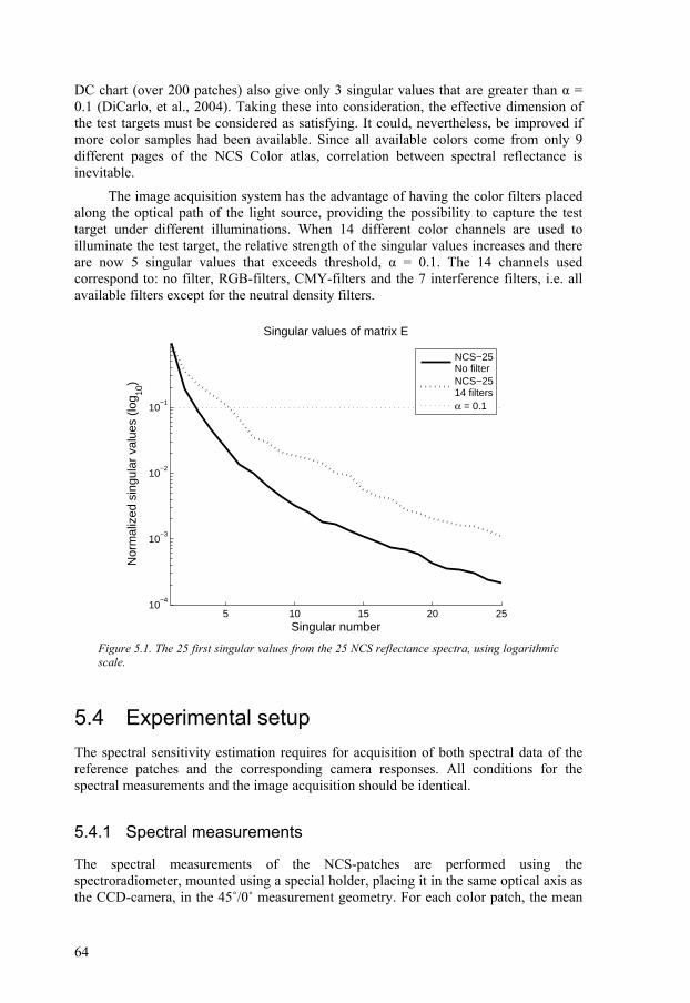
64

DC chart (over 200 patches) also give only 3 singular values that are greater than α = 0.1 (DiCarlo, et al., 2004). Taking these into consideration, the effective dimension of the test targets must be considered as satisfying. It could, nevertheless, be improved if more color samples had been available. Since all available colors come from only 9 different pages of the NCS Color atlas, correlation between spectral reflectance is inevitable.

The image acquisition system has the advantage of having the color filters placed along the optical path of the light source, providing the possibility to capture the test target under different illuminations. When 14 different color channels are used to illuminate the test target, the relative strength of the singular values increases and there are now 5 singular values that exceeds threshold, α = 0.1. The 14 channels used correspond to: no filter, RGB-filters, CMY-filters and the 7 interference filters, i.e. all available filters except for the neutral density filters.

Figure 5.1. The 25 first singular values from the 25 NCS reflectance spectra, using logarithmic scale.

5.4 Experimental setup The spectral sensitivity estimation requires for acquisition of both spectral data of the reference patches and the corresponding camera responses. All conditions for the spectral measurements and the image acquisition should be identical.

5.4.1 Spectral measurements

The spectral measurements of the NCS-patches are performed using the spectroradiometer, mounted using a special holder, placing it in the same optical axis as the CCD-camera, in the 45˚/0˚ measurement geometry. For each color patch, the mean

5 10 15 20 2510

−4

10−3

10−2

10−1

Singular number

Nor

mal

ized

sin

gula

r va

lues

(lo

g 10)

Singular values of matrix E

NCS−25No filterNCS−2514 filtersα = 0.1

65

reflectance spectrum from 5 sequential measurements is computed. The spectral data are in the interval 380 to 780 nm sampled at 4 nm intervals, giving N = 101.

The reflectance measurements are performed using the illuminant only, without any filter. From the measured reflectance of the NCS patches, the resulting spectral data Ek(λ) for channel k = 2,…,14 is then computed using the known spectral transmittance for each filter (Sec. 4.4). The 14 channels correspond to: no filter, the RGB-filters, CMY-filters and the 7 interference filters. The spectral data of the 25 reference color patches, using all 14 color-channels, is collected into the 101× 350 matrix E, with each column containing the spectral data of color patch p, filter k.

5.4.2 Image acquisition

For each color target, 14-chanel images have been captured, using the same 14 color filters as for the spectral computations, and the same 45˚/0˚ measurement geometry. The mean is computed from 5 sequential images, captured at slightly different locations, by moving the xy-table on which the image is placed. Because of the high magnification of the optics, the images have been captured slightly out of focus, to prevent small irregularities in the surface to influence the result. The exposure times used have been individually calibrated for each channel.

5.4.3 Processing the images

As a pre-processing step, all images are corrected for dark current and electronic gain, as described in Sec. 4.6.4. The channel-dependent normalization factors, ak, used in Eq. 4.5 are chosen as:

kk Et

Eta 1= (5.23)

where Et1 is the calibrated exposure time for channel 1 (i.e. the illuminant without any filter) and Etk is the exposure time used for channel k. In this way, the camera response values are adjusted according to the channel-dependent exposure times, and normalized against the mean camera response for the white reflectance standard.

From the corrected and normalized images Ick (x,y), the mean values are computed for each channel k and used as the camera response value, dk,p, for NCS colors p = 1,…,25. When computing the mean values it has been controlled that no pixel value deviates more than 5% from the mean, to prevent any defective pixels to affect the results. The resulting camera response values dk,p are collected into the 350-component vector d, used for the spectral sensitivity estimation.

5.5 Results Since the real spectral sensitivity function is unknown, the estimated sensitivity is evaluated by using the forward characterization model to predict device response values, d̂ , from the known spectral data, as:

66

ˆ ˆt=d E s (5.24)

where E is the N × P matrix with the columns corresponding to spectral measurements of each color sample, and ŝ the estimated spectral sensitivity.

For the evaluation, the remaining NCS color patches has been used, predicting the device response for all the 14 color channels. The predicted response values, d̂ , are then compared with the real, measured device responses, d, to compute the following error metrics:

2

1

RMSerror1 ˆ

P

i ii

d dP =

= −∑ (5.25)

and the 2

1

Relative RMSerrorˆ1 P

i i

i i

d dP d=

−= ∑ (5.26)

5.5.1 Manufacturer data

The manufacturers of the optics and CCD camera respectively, have provided data representing ‘typical’ curves for the CCD quantum efficiency and spectral transmittance of the optics. The data is available only in graphical form and the resolution is limited (Appendix B). To evaluate the accuracy of the data provided by the manufacturers, data has been collected manually from the graphs, and then cubically interpolated. The data for the optics and CCD have been combined together into the camera sensitivity function according to Eq. 5.1.

The estimation errors when using the manufacturer data to predict the camera response values from real spectral data were relatively small. Clearly the data provided by the manufacturer is fairly accurate, with typical curves that better represent the actual devices than for consumer products, where the variance between the individual devices is usually large (DiCarlo, et al., 2004). Considering the good quality of the data provided by the manufacturers, the assumption was then made that the real function should be similar, i.e. it is most likely both uni-modal and smooth. The sensitivity function derived from the manufacturer data is used as a reference to see if it is possible to achieve a more accurate estimate of the spectral sensitivity function.

5.5.2 PI and PE solutions

The unconstrained pseudo-inverse (PI) solutions have been derived using absolute and relative RMS as objective function, according to Eqs. 5.5 and 5.19. As expected, the resulting estimations are very noisy. Even though providing low RMS-errors, their magnitude, negative values and non-smoothness make them practically useless as an approximation of the true camera sensitivity function.

The resulting spectral sensitivity function has also been estimated, using the principle eigenvector (PE) method, for the first 1 to 9 principle eigenvectors included in

67

the inversion. The smoothness of the estimated function decreases with increasing number of PE’s, due to the increasing sensitivity to noise. The estimates are neither uni-modal nor generally smooth enough to be considered as realistic candidates. They are however all positive, without explicitly using positivity as a constraint. The spectral sensitivity estimations and the resulting prediction errors for the unconstrained PI and PE methods are given in Appendix B.

5.5.3 Constrained solutions

To ensure smooth camera sensitivity functions; the estimations are represented as linear combinations of Fourier basis, according to Equations 5.13, and to ensure positivity, the constraint according to Equation 5.12 is used. To allow for a greater freedom of the sensitivity estimation, booth the number of basis and the cycle length used are varied compared to previous work where the cycle length is fixed and equal to the wavelength interval used (Barnard & Funt, 2002; Finlayson & Hubel, 1998). The number of base-functions, l, is varied between 1:15, and the cycle length, c, is 100:10:490 nm, giving totally 600 possible estimations, for each different number of PE’s included.

To select the optimal estimates from all the candidates derived, selection criterions are needed. The best results were found by combining the two error metrics, using the absolute RMS error as objective function in the regression, and the relative RMS error as criterion for selection. Furthermore, the uni-modality constraint was used as a criterion for selection. It was found that the uni-modality worked better as a criterion for selection, compared to when it was incorporated as a constraint in the regression, which produced unrealistic, flat curves. It seems, with this approach, that the number of principal eigenvectors included is of little importance.

As an alternative to ensuring smoothness by using Fourier basis, the method of adding a regularization term to the objective function according to Eqs. 5.16 - 5.17, has been implemented. Barnard and Funt (2002) claimed that the value of the coefficient γ is “easily found by trial and error”. However, it is clear that the RMS error will increase with increasing weight, γ, in the objective function. Hence, there must be a manual trade-of between low RMS-error and the acceptable smoothness.

The same approach as for the Fourier basis is adapted, i.e. using the absolute RMS as objective and searching for the lowest relative RMS-error. The number of eigenvectors included in the inversion has a greater impact on the result, compared to the Fourier basis approach. The RMS errors decreases with increasing number of PE included, but so does the non-smoothness. The best result for the candidates that are smooth and uni-modal, is found when PE = 3 and γ = 30. The spectral sensitivity estimates for different number of PE’s and the resulting prediction errors are given in Appendix B, for the Fourier basis approach, as well as usinig the regularization term.

Table 5.1 lists the predicted errors of the spectral sensitivity estimations considered as the best candidates, using Fourier basis and regularization term, respectively. For comparison, the results for the function derived from manufacturer data are included. The corresponding sensitivity functions are displayed in Fig. 5.2.

68

Table 5.1. The resulting prediction errors for the best estimates of the camera sensitivity function compared to the data provided by the manufacturer

Manufacturerdata

Fourier basis Regularization term

RMS-error 5.45 10-4 2.26 10-4 2.33 10-4 Relative RMS-error 0.038 0.0149 0.0184 Mean error 0.012 0.0070 0.0072 Max error 0.13 0.0965 0.0972

Figure 5.2. The best estimates of the camera sensitivity function compared to the estimate derived from data provided by the manufacturer.

Clearly, both the estimated sensitivity functions show resemblance to the function

derived from manufacturer data, being uni-modal and smooth. Table 5.1 reveals that both the estimated functions outperform the manufacturer data in terms of all the error metrics analyzed. The best choice is the estimation based on Fourier basis, where both absolute and relative RMS errors are more than halved compared to manufacturer data. The maximal error for the predicted device response to the reference colors, using 14 color-channels, is reduced to 0.097 (images normalized in the range [0,1]) and the mean is as low as 0.007.

5.6 Summary and discussion The spectral sensitivity function, including the spectral transmittance of the optics and the quantum efficiency of the CCD, has been estimated using a set of 25 carefully selected NCS colors. By relating the measured reflectance spectra of the reference colors to the corresponding device responses, the sensitivity function was derived using least squares regression. The principle eigenvector method was used to reduce the noise

400 450 500 550 600 650 700 7500

0.05

0.1

0.15

0.2

0.25

0.3

0.35

0.4

0.45

Wavelength, λ (nm)

Est

imat

ed c

amer

a se

nsiti

vity

Manufacturer dataFourier basisRegularization term

69

sensitivity, and a priori knowledge on the nature of camera sensitivity, such as positive valued, smoothness and uni-modality, was used as constraints in the regression.

The estimated camera sensitivity function considered as the best candidate was the result from minimizing the absolute RMS error, using the PE-method with positivity constraint and Fourier basis to ensure smoothness. Out from the large number of estimations, the best candidate was selected using the relative RMS error and the uni-modality requirement, as selection criterion. The selected sensitivity function is similar to the function derived from the manufacturer data, but reduces the prediction errors more than a half. When the estimated sensitivity function was used to predict the response to a set of test colors, independent from the ones used in the estimation, the mean prediction error was 0.007 with the maxim 0.097 (camera values in the range [0,1]).

Besides the method employed in this study, there are other approaches to derive the spectral sensitivity function. It is possible to derive a more accurate estimate from the device response to monochromatic light obtained by using a monochromator. Another approach uses neural networks to estimate the spectral sensitivity function from color targets. The third uses a set theoretical formulation to express the constraints as convex sets and use the iterative technique projection onto convex sets (POCS) to generate the sensitivity function (Sharma & Trussel, 1996).

The spectral sensitivity function that was estimated will be used in the following chapter for reconstructing spectral data from device response. It was the last component of the spectral image acquisition model, which is now complete.

70

71

Chapter 6 6 Model-based spectral reconstruction

Model-based spectral reconstruction

6.1 Introduction 6.2 Theory of spectral reconstruction 6.3 Experimental setup 6.4 Metrics for spectral comparison 6.5 Experimental results 6.6 Summary and discussion

72

73

6.1 Introduction After estimating the spectral sensitivity function for the camera in Chapter 5, the spectral image acquisition model is complete. The model describes the forward characterization function predicting the device response to a known spectral input. However, the inverse characterization function is often required, deriving device-independent color data for an object, using the recorded device response. In colorimetric imaging, the device-independent representations are typically CIEXYZ or CIELAB, and in multispectral imaging estimations of the spectral reflectance are derived.

The focus in this chapter is multispectral imaging, using model-based characterization. The aim is to reconstruct the spectral reflectance of objects from the recorded device response, by inverting the spectral model of the image acquisition system. As the physical representation of color of an object, spectral reflectance is completely independent of the characteristics of the image acquisition system. From the spectral reflectance data it is straight forward to convert the data to colorimetric representations, as well as to render the image under different illuminations.

Compared to empirical characterization, model-based characterization is more general and allow for applications to arbitrary combinations of media and colorants. The accuracy of the spectral reconstructions depends on the noise levels, and on how well the spectral model reflects the real characteristics of the image acquisition system, i.e. it is not dependent on a training set of color samples.

Spectral reconstruction is performed using both trichromatic (RGB) and multi-channel images, to evaluate the difference in performance. A priori knowledge on the smooth nature of spectral reflectances is exploited, by representing the spectra as linear combinations of different basis functions. The metrics used to evaluate the results, include the spectral RMS difference, as well as the Euclidian distance in CIEXYZ color space, and the CIE 1976 and 1994 color differences in CIELAB.

6.2 Theory of spectral reconstruction Recall the forward spectral image acquisition model, describing the response of the device by modeling the physical characteristics of all the components involved in the

74

image acquisition process (repeated in Eq. 6.1). The device response, dk, for the k:th channel is, for each pixel, given by:

( ) ( ) ( ) ( )k k kV

d I F R S dλ

λ λ λ λ λ ε∈

= +∫ (6.1)

Having obtained the spectral characteristics of all the components, the

characteristics of the image acquisition system can be represented by a spectral transfer function (Farell et al, 1999). The spectral transfer function, Wk(λ), describes the spectral characteristics for each channel k, including the illuminant, the camera sensitivity and the filter transmittance, as:

( ) ( ) ( ) ( )k kW I F Sλ λ λ λ= (6.2)

Denote the spectral signal as a discrete N-component vector, sampled at wavelengths λ1,…, λN, and let W be the N × K matrix in which each column describes the spectral transfer function of channel k. Then the camera response vector, d, for a sample with spectral reflectance r is given by:

t=d W r (6.3)

When inverting the model, we seek the N × K reconstruction matrix M that best reconstructs the spectral reflectance,r , from the camera response d, as:

=r Md (6.4)

6.2.1 Pseudo-inverse solution

The most straightforward approach to derive the reconstruction matrix is to simply invert Eq. 6.4, using the pseudo-inverse approach. This gives the reconstruction operator:

( )t −=r W d (6.5)

where (Wt)- denotes for the More-Penrose pseudo-inverse of Wt. Thus, the pseudo-inverse reconstruction operator is given by:

0 ( )t −=M W (6.7)

Generally, the pseudo-inverse reconstruction is sensitive to noise, which makes the approach not always useful in practices. When K < N, i.e. the number of color channels K is less than the number of spectral sampling points N, the matrix W is of insufficient rank and the algebraic equations are underdetermined. Further more, this method minimizes the Euclidian distance in the camera response domain (i.e. between d and Wt r ), which does not necessarily mean that the reconstructed spectrum will be close to the real spectrum. (Hardeberg, 2001)

75

6.2.2 Basis functions

Another approach is to instead seek another reconstruction matrix, M1, which minimizes the Euclidian distance between the reconstructed spectrum and the original spectrum (Hardeberg, 2001). The vast majority of reflectance spectra for real and man-made surfaces are smooth functions of wavelength (Maloney, 1986; Connah, et al., 2001). By exploiting the priori information, we can assume that the reflectance can be represented by a linear combination of a set of smooth basis functions, B = [b1,b2…bp]. With this assumption, the reflectance can be represented using the vector of coefficients, a , as:

=r Ba (6.8) Hence, r can be obtained from a (using Eqs. 6.3, 6.4, and 6.8), as:

1 1 1t t= = =r M d M W r M W Ba (6.9)

Then, the ideal expression =r r , becomes:

1t =M W Ba Ba (6.10)

Assuming the basis B represents a statistically significant representation of the reflectances likely to be encountered, Eq. 6.10 should be true for any a, and hence:

1t =M W B B (6.11)

This gives the reconstruction operator M1, minimizing the RMS spectral error of the reconstructed spectrum. (Hardeberg, 2001)

( ) 11

−= WBBWWBBM ttt (6.12)

The base functions, B, can consist of a set of real, measured spectral reflectances, which then should be representatives to the reflectance of samples that are likely to be encountered in the image acquisition system. To reduce the noise sensitivity, the principle eigenvector method can be applied to the set of spectral basis, as described in Sec. 5.2.3. An alternative to spectral basis is to simply let B be a set of Fourier basis functions.

6.3 Experimental setup In multispectral imaging, each pixel should contain the spectral information about the scene, combining the strengths of spectral and spatial resolution. However, when experimenting on spectral reconstruction, it is necessary to evaluate the results by comparing to spectral measurements. Hence, the comparison must be made using color samples which have a constant color over some area, which can be measured by a spectroradiometer or spectrophotometer.

76

For reference color samples to evaluate the results, 25 color patches from NCS are used. The spectral reflectance values of the patches have been measured using a spectroradiometer. Correspondingly, the camera response values have been acquired under the identical conditions, using the 45°/0° geometry. The setup for the spectral measurements and the image acquisition is identical to Sec. 5.4, and so is the processing of the captured images.

6.4 Metrics for spectral comparison To evaluate the quality of the reconstructed spectral reflectance, metrics are needed to compute the closeness to the real spectra. Depending on the shapes and magnitudes of the spectral reflectance curves, different metrics can result in very different results (Imai et al., 2000). The spectral RMS error corresponds to the Euclidian distance, in spectral reflectance space, between the original and the reconstructed spectra. It is simple, widely used and well suited for comparison of physical stimuli, but it does not correlate to the perceived color difference. Even though the CIE color difference formulas described in Sec. 2.2.7, ∆Eab and ∆E94, are not directly designed for evaluating spectral matches, they provide a measure of the perceived color difference under a given illuminant, based on characteristics of the human visual system. Their main drawback, however, is that they provide poor correlation to the spectral similarity for metameric colors. Other metrics include the metamerism indices, which compare to which extent two spectra differs under different illuminants and observers (Sec. 2.2.5).

For a thorough survey and comparison of different metrics used for spectral estimations, we refer to Imai et al. (2002). According to Imai there is no metric that suits for all purposes and combinations of different metrics should be used to take advantage of each metric.

We choose to present the RMS spectral reconstruction error, together with the Euclidian difference in CIEXYZ color space, ∆XYZ. Furthermore, the CIE color differences ∆Eab and ∆E94, under the standard illuminants D65 and A, are computed. For each metric, the maximum and mean values of the 25 reference samples are presented, as well as the 95th percentile, i.e. the value below which 95% of the samples lay.

6.5 Experimental results Experiments on inverting the spectral model to reconstruct spectral reflectance have been performed for the 25 NCS color patches. Spectral reflectance data is reconstructed using the operators M0 and M1 according to Eqs. 6.7 and 6.12, using both multi-channel images (from the 7 interference filters) and trichromatic (RGB) images. Concerning the basis functions, B, both Fourier basis and spectral basis are evaluated. With the Fourier basis, the best results were obtained using 5 base functions, which is used in all of the following results.

For the spectral basis, the database provided by NCS, containing spectral reflectance of 1750 different color samples, are used. The spectral reflectance data available from NCS is in the range 400 to 700 nm. For the results to be directly comparable, the spectral data has been cropped to the range 400 to 700 nm even for the

77

PI-method and Fourier basis. It is worth noticing that due to the very low energy available from the illuminant at both ends of the visible spectrum, the data outside this interval is noisy and the reconstruction error decreases by excluding data outside this range. To reduce the sensitivity to noise, the principle eigenvector (PE) method has been used, as described in Sec. 5.2.3. The best results were obtained when representing the spectral basis by the singular vectors corresponding to the 5 most significant singular values.

The RMS spectral reconstruction errors for the 25 reference colors are given in Table 6.1, together with their Euclidian distances in the CIEXYZ color space. The CIELAB differences ∆Eab and ∆E94 are collected in Table 6.2.

Table 6.1. Spectral reconstruction errors, expressed as RMS difference in spectral space, and the Euclidian distance in CIEXYZ space, ∆XYZ.

Data

Method

Max

RMS Mean

95%

Max

∆XYZ Mean

95%

PI 0.0706 0.0230 0.0598 24.27 13.19 23.60 Spectral 0.0041 0.0014 0.0040 10.44 3.978 9.591

RGB

Fourier 0.0155 0.0049 0.0141 7.749 3.603 6.997 PI 0.0092 0.0030 0.0072 3.989 1.103 3.828 Spectral 0.0039 0.0012 0.0030 4.805 1.331 4.366

D65

Multi

Fourier 0.0040 0.0011 0.0027 3.735 1.287 3.723 PI 10.16 6.755 9.634 Spectral 11.34 4.378 10.97

RGB

Fourier 6.699 2.682 6.357 PI 3.214 0.934 3.151 Spectral 3.224 0.960 3.158 Ill

umin

ant

A

Multi

Fourier 3.758 1.091 3.685

Table 6.2. Colorimetric reconstruction errors. CIE 1976 color difference, ∆Eab and CIE 1994 color difference ∆E94,.

Data

Method

Max

∆Eab Mean

95%

Max

∆E94 Mean

95%

PI 24.35 14.80 22.09 17.00 9.559 16.03 Spectral 15.87 4.170 10.37 6.207 2.726 6.175

RGB

Fourier 18.75 8.287 18.68 10.95 5.075 10.56 PI 4.364 1.529 3.145 1.911 0.974 1.860 Spectral 4.218 1.816 3.303 2.053 1.130 1.985

D65

Multi

Fourier 7.271 2.112 5.780 2.813 1.216 2.730 PI 15.24 8.789 13.78 10.16 6.755 9.634 Spectral 11.24 4.350 10.53 7.638 3.083 6.873

RGB

Fourier 14.34 5.937 14.11 7.506 3.691 7.173 PI 3.858 1.331 3.115 1.813 0.855 1.801 Spectral 4.469 1.802 3.295 1.902 1.072 1.831 Ill

umin

ant

A

Multi

Fourier 5.983 2.189 4.860 2.995 1.331 2.412

Figure 6.1 displays the reconstructed spectral reflectance from RGB-images, using three NCS colors as examples. The corresponding results using multi-channel images are given in Fig. 6.2.

78

Figure 6.1. Reconstructed spectral reflectance from RGB-images. Full lines are measured spectral reflectance, the dashed lines are reconstructed.

For the RGB images, the pseudo-inverse solutions are eventually useless (Fig. 6.1), resulting in mean errors close to 15 ∆Eab. The results improved when using base functions, with the best results obtained for spectral basis. However, a mean ∆Eab difference of 4 and a maximum of 14 are still too high for the method to be considered as useful for multispectral imaging.

Figure 6.2. Reconstructed spectral reflectance from multi-channel images. Full lines are measured reflectance spectra, the dashed lines are reconstructed.

400 500 600 7000

0.5

1Pseudo−inverse

400 500 600 7000

0.5

1Spectral basis

400 500 600 7000

0.5

1Fourier basis

400 500 600 7000

0.5

1

Est

imat

ed s

pctr

al r

efle

ctan

ce

400 500 600 7000

0.5

1

400 500 600 7000

0.5

1

400 500 600 7000

0.5

1

400 500 600 7000

0.5

1

Wavelength, λ (nm)400 500 600 7000

0.5

1

400 500 600 7000

0.5

1Pseudo−inverse

400 500 600 7000

0.5

1Spectral basis

400 500 600 7000

0.5

1Fourier basis

400 500 600 7000

0.5

1

Est

imat

ed s

pctr

al r

efle

ctan

ce

400 500 600 7000

0.5

1

400 500 600 7000

0.5

1

400 500 600 7000

0.5

1

400 500 600 7000

0.5

1

Wavelength, λ (nm)400 500 600 7000

0.5

1

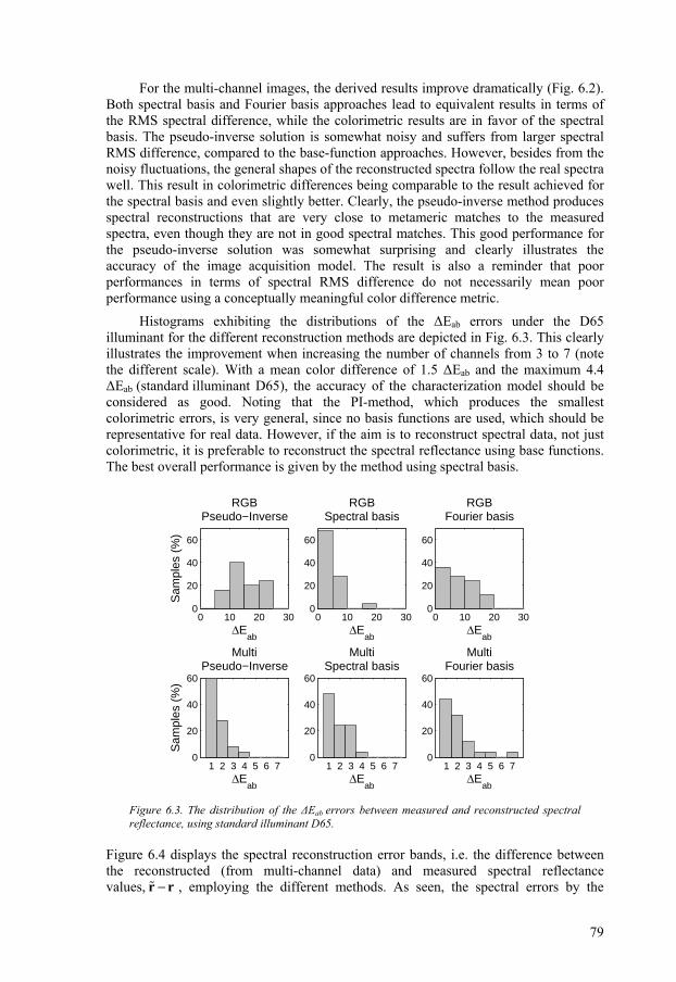
79

For the multi-channel images, the derived results improve dramatically (Fig. 6.2). Both spectral basis and Fourier basis approaches lead to equivalent results in terms of the RMS spectral difference, while the colorimetric results are in favor of the spectral basis. The pseudo-inverse solution is somewhat noisy and suffers from larger spectral RMS difference, compared to the base-function approaches. However, besides from the noisy fluctuations, the general shapes of the reconstructed spectra follow the real spectra well. This result in colorimetric differences being comparable to the result achieved for the spectral basis and even slightly better. Clearly, the pseudo-inverse method produces spectral reconstructions that are very close to metameric matches to the measured spectra, even though they are not in good spectral matches. This good performance for the pseudo-inverse solution was somewhat surprising and clearly illustrates the accuracy of the image acquisition model. The result is also a reminder that poor performances in terms of spectral RMS difference do not necessarily mean poor performance using a conceptually meaningful color difference metric.

Histograms exhibiting the distributions of the ∆Eab errors under the D65 illuminant for the different reconstruction methods are depicted in Fig. 6.3. This clearly illustrates the improvement when increasing the number of channels from 3 to 7 (note the different scale). With a mean color difference of 1.5 ∆Eab and the maximum 4.4 ∆Eab (standard illuminant D65), the accuracy of the characterization model should be considered as good. Noting that the PI-method, which produces the smallest colorimetric errors, is very general, since no basis functions are used, which should be representative for real data. However, if the aim is to reconstruct spectral data, not just colorimetric, it is preferable to reconstruct the spectral reflectance using base functions. The best overall performance is given by the method using spectral basis.

Figure 6.3. The distribution of the ∆Eab errors between measured and reconstructed spectral reflectance, using standard illuminant D65.

Figure 6.4 displays the spectral reconstruction error bands, i.e. the difference between the reconstructed (from multi-channel data) and measured spectral reflectance values, −r r , employing the different methods. As seen, the spectral errors by the

0 10 20 300

20

40

60

∆Eab

Sam

ples

(%

)

RGBPseudo−Inverse

0 10 20 300

20

40

60

∆Eab

RGBSpectral basis

0 10 20 300

20

40

60

∆Eab

RGBFourier basis

1 2 3 4 5 6 70

20

40

60

∆Eab

Sam

ples

(%

)

MultiPseudo−Inverse

1 2 3 4 5 6 70

20

40

60

∆Eab

MultiSpectral basis

1 2 3 4 5 6 70

20

40

60

∆Eab

MultiFourier basis

80

pseudo-inverse approach are periodic, with small errors mainly occurring at wavelengths where the multi-channel filters have their peak transmittance (compare to Fig. 4.6). The error band representing spectral basis reveals that the largest errors occur at the two ends of the visible spectrum, especially at the red end where the reconstructed reflectance is generally overestimated. The results from Fourier basis show large errors at the both ends of the visible spectrum as well, but even in the band around 650 nm.

Figure 6.4. Spectral reconstruction error band for the 25 NCS colors, using the different reconstruction operators for multi-channel images.

6.6 Summary and discussion The inverse characterization function has been derived using a model-based approach, i.e. by inverting the spectral model of the image acquisition process, derived in the previous chapters. The result of the inversion is a set of spectral reconstruction matrices, allowing for the acquisition of multispectral images, i.e. to reconstruct the spectral reflectance from the recorded device response. To exploit a priori knowledge on the smooth nature of spectral reflectance, basis functions have been used to improve the accuracy of the inversion. The basis functions evaluated consist of Fourier basis and a large set of real reflectance spectra from the NCS, combined with the principle eigenvector method. The spectral reconstruction methods have been tested using multi-channel images, as well as trichromatic RGB-images. The results have been evaluated by comparing the reconstructed spectral reflectance to measurements by a spectroradiometer, for a set of 25 NCS color patches.

The results show that the trichromatic RGB signals are insufficient in reconstructing the spectral and colorimetric data. The best results, using the spectral basis, produced a mean CIE 1976 color difference of 4 ∆Eab with the maximum 14 ∆Eab.

When using multi-channel images, the improvement was significant, both in terms of colorimetric differences and in the RMS spectral reconstruction error. The best

400 450 500 550 600 650 700

−0.2

0

0.2

Pseudo−inverse

400 450 500 550 600 650 700

−0.2

0

0.2

Ref

lect

ance

rec

onst

ruct

ion

erro

r

Spectral basis

400 450 500 550 600 650 700

−0.2

0

0.2

Wavelength, λ (nm)

Fourier basis

81

results in terms colorimetric differences were obtained for the simple pseudo-inverse solution, producing a mean color difference of 1.5 ∆Eab and the maximum 4.4 ∆Eab. The results using spectral basis were comparable in terms of ∆Eab and significantly better in terms of the RMS spectral difference. Fourier basis produced good results in RMS spectral difference, but slightly worse in terms of the CIE color differences.

The results indicate that if the aim is to derive colorimetric data only, the PI-method is sufficient. The PI-method is very general, since no basis functions are used, which should then be good representatives for the spectra likely to be encountered. However, the PI-method produces spectral reconstructions that are good metameric matches, not good spectral matches. Hence, for multispectral imaging, i.e. when reconstructing spectral data from the device response, the methods using base functions are required. The best overall performance is given by the method using spectral basis.

Possible ways of improving the accuracy of the model-based characterization could be to use Wiener estimation techniques, to take into account the signal dependent acquisition noise (Haneishi, et al, 2000). It would be desirable to verify the results using a larger set of test colors, preferably of various media and colorants. Notice that the spectral basis used consist of principle eigenvectors from the database of NCS color, which should be favorable when reconstructing reflectance spectra of NCS patches. For other media, it would probably be beneficial to use other spectral basis, e.g. including the reflectance for the substrate and the printing inks in the spectral basis, for multispectral imaging of color prints.

82

83

Chapter 7 7 Colorimetric and spectral reconstruction using empirical characterization

Colorimetric and spectral reconstruction using empirical characterization

7.1 Introduction 7.2 Media dependency 7.3 Methodology 7.4 Experimental setup 7.5 Experimental results 7.6 Summary and discussion

84

85

7.1 Introduction For comparison to the results using model-based characterization to reconstruct spectral and colorimetric data described in Chapter 6, experiments are performed using empirical characterization. The spectral characteristics of the image acquisition system are ignored and the inverse characterization functions are derived based on the recorded device response for a training set of color samples. By relating the device response to spectral and colorimetric measurements, the characterization functions are derived using least squares regression techniques, as described in Sec. 3.6.

Beside from colorimetric regression, mapping device values directly to CIEXYZ and CIELAB using linear and polynomial regression, experiments are also made on reconstructing spectral reflectance by least squares regression. The regression is performed using both RGB and multi-channel images. To evaluate the result, a set of 50 test colors is used, independent from the training set used to derive the mappings. The influence of the size of the training set is examined and so is the performance of the derived functions when used for color samples of different media and colorants.

The spectral reconstructions are evaluated using the spectral RMS difference, and the colorimetric estimations by using the Euclidian distance in CIEXYZ color space, and the CIE 1976 and 1994 color difference formulas. The colorimetric differences have been computed using both the standard illuminants A and D65. However, to keep the number of pages of the chapter manageable, some results have been moved to the appendix. The discussions are based on the results for D65, which are presented in this chapter. The results for standard illuminant A can be found in Appendix C.

7.2 Media dependency The characterization functions derived using empirical approaches will be optimized only for a specific set of conditions, including the illuminant, the media and the colorant. Once the conditions change, e.g. capturing images of a different substrate or a different print mechanism, the characterization has to be re-derived in order to obtain good accuracy (Pan et al., 2001; Andersson et al., 2003). The dependency on the illuminant is natural and is often not an issue when the light source is fixed and can be considered as a property of the system. However, the fact that the characterization function is also media- and colorant dependent is a major drawback, preventing the

86

characterization function from being applied to arbitrary combinations of media and colorants.

The media- and colorants dependency can be explained from the so-called eye-camera metamerism (Hong & Lou, 2000), also referred to as device metamerism (Cheung, et al., 2005). Recall from Chapter 2 that two color samples are metameric when giving the same tristimulus values for a specific illumination condition, even though they are spectrally different. When the spectral responses of an imaging device are different from the color matching functions, i.e. the device is not colorimetric; colors that are metameric in terms of tristimulus values are not necessarily metameric with respect to the imaging sensors. This means that metameric color samples, which give the same tristimulus values under a given illuminant, may generate different device response values under the same illuminant. Conversely, two spectrally different samples, which are metameric for the imaging system only, will result in the same device response and thus the same colorimetric values after applying the characterization function, even though they are not a metameric match in terms of tristimulus values, under the given illuminant.

The magnitude of the color mismatch is related to the difference in spectral reflectance properties of the samples and the consequence of this eye-camera metamerism is that the mappings derived in the characterization process will be media dependent, i.e. optimal only for the combination of media and colorants used for the characterization. Since empirical characterization generally requires a large number of measurements to obtain device data and the corresponding colorimetric values of the training samples, this media dependence is a drawback if the characterization function is to be used for arbitrary combinations of media and colorants.

7.3 Methodology In the following, recall the workflow for empirical characterization of input devices, given in Sec. 3.4. The aim is to derive the inverse characterization function, mapping device response values {di} to device-independent colorimetric representations {ci} and spectral reconstructions i{ }r , using least squares regression techniques.

7.3.1 Colorimetric regression

A common approach for empirical characterization is to use linear or polynomial regression from device RGB values to CIEXYZ (see for example Hong & Lou, 2000). From the XYZ values it is then straight forward to compute the CIELAB values using standard formulae. The drawback with using regression to CIEXYZ is that the RMS error in XYZ color space, which is minimized in the regression, is not closely related to the perceived color difference. If the final aim is to derive data in CIELAB color space, it is therefore preferable to use regression directly in the CIELAB domain, i.e., to minimize the ∆Eab difference in the regression, which provides a better correspondence to the visual color difference (Hardeberg, 2001). Since the relationship between device RGB data and CIELAB color space is not linear, a non-linear pre-processing step of the RGB values using a cubic root function is proposed, i.e. using R1/3, G1/3, B1/3 in the regression (Hardeberg, 2001). The cubic root function originates from the CIELAB

87

transformation, which involves a cubic root function of the XYZ tristimulus values (Eqs 2.8 – 2.10).

7.3.2 Spectral regression

Even though empirical approaches are mainly used to derive mappings to colorimetric data, CIEXYZ or CIELAB, there have been attempts to reconstruct spectral reflectance (Solli, et al., 2005). Instead of seeking the relationship between device response values and colorimetric values, we now look at the linear relationship r = dA, where r is the spectral reflectance N-component vector for a color sample, d is the m-component vector representing the corresponding device response, and A is a m × N spectral reconstruction matrix. If the spectral reflectance for a set of T training samples {ri} are collected into a T × N matrix R = [r1, …,rT] and the device responses {di} into a T × m matrix D = [d1, …,dT], then the linear relationship is given by (compare to Eq. 3.4): R = DA (7.1) and the optimal reconstruction matrix A is then given by:

1( ) ( )t t− −= =A D D D R D R (7.2) where (D)- is the Moore-Penrose pseudo-inverse of D. The spectral reflectance can then be reconstructed from camera response values as:

=r dA (7.3)

Note that the spectral reconstruction matrix, A, is now derived entirely based on the recorded device response to a set of training samples, i.e. ignoring the spectral characteristics of the imaging system.

7.3.3 Evaluation

Figure 7.1 summarizes the different approaches for deriving colorimetric and spectral reflectance values, and the way which the results are evaluated. From the recorded device response, d, (either RGB or multi-channel images), the spectral reflectance can be reconstructed, using linear regression. The spectral estimation is compared to the spectral reflectance measured by a spectroradiometer, to compute the RMS spectral difference.

From the spectral reflectance, the tristimulus values CIEXYZ can be computed using the CIE color matching functions (Eq. 2.3), under a chosen illuminant. The XYZ values can alternatively be derived directly by colorimetric regression from the device response. The estimated tristimulus values are evaluated by computing the Euclidian distance to the XYZ values computed from the measured spectral reflectance.

From the XYZ tristimulus values it is then possible to compute CIELAB coordinates, according to Eqs 2.14 – 2.16. Alternatively, the CIELAB values can be derived using direct regression from device response, with or without the proposed pre-

88

processing step. The CIELAB values are evaluated using the color difference formulas ∆Eab and ∆E94, as described in Sec. 2.2.7.

Figure 7.1. The different approaches for deriving colorimetric and spectral reflectance values from the recorded device response.

7.4 Experimental setup

7.4.1 The training set

Being rather time consuming in spectral measurements using a spectroradiometer, as well as in image acquisition, it is desirable to use as few test colors as possible, while achieving a satisfactory result. It has been suggested that a suitable number of test colors for polynomial regression is 40-60 training samples, with no significant improvement of the accuracy obtained by further increasing the size of the training set (Hong & Lou, 2000). Similarly, it has been shown that reducing the training set from 288 to 54 test colors gives only a very small increase in the estimation error (Hardeberg, 2001). The basic and most important demand is that the number of training colors is larger than the number of parameters in the model, ensuring that the system is not underdetermined.

As training set for the regression we use a set of 50 test colors, printed on HP Photo-matte paper by a HP 10PS inkjet printer (Solli, 2004). The reason for not using NCS colors, as with the model-based approach, was simply that the number of available NCS color patches was not sufficient to be used both as training set and for evaluation. To investigate the influence of the size of the training set on the characterization, experiments are performed on reducing the number of training colors.

For the evaluation of the derived characterization function, 50 randomly selected colors are used, printed using the same substrate and conditions as the training set.

R(λ)

Image acquisition

Spectral measurements

Spectral reflectance

Spectral reflectance (estimated)

CIE XYZ

CIE L*a*b*

CIE XYZ (est)

CIE L*a*b* (est)

Device response d

CMFs

CMFs

Transform

Transform

Spec

tral e

rror

Col

orim

etric

err

or

Col

or d

iffer

ence

Est

imat

ions

RM

S

∆XY

Z

∆E a

b, ∆

E 94

Pre-processing

89

Since characterization functions derived by least squares regression will always be optimized for the specific training set, it is important to use a different set of test colors for the evaluation. An independent set of evaluation colors guards against a model that overfits the training set, giving unrealistically good results (Cheung, 2005).

7.4.2 Setup

To prevent the halftone pattern of the printed test colors from appearing in the images because of the large magnification, the images are captured slightly out of focus, using the shortest extension available. In all other aspects, the setup for the spectral measurements as well as the acquisition and processing of the images, is identical to the setup for the model-based characterization, as described in Sec. 5.4.

7.4.3 Choice of the approximation functions

Beside from the basic linear regression, experiments are performed using polynomial regression to CIEXYZ and CIELAB from RGB and multi-channel images, as described in Sec. 3.6. The recorded device response is arranged into different polynomial Q-component vectors, p, and the optimal matrix of polynomial weights are found using Eq. 3.10. The regression to CIELAB is performed using the device response directly, as well as by using the proposed non-linear pre-processing step.

RGB data Besides the basic linear regression, we evaluate the following polynomials as approximation functions for trichromatic RGB-images:

2 2 21 [1, , , , , , , , , ]R G B R RG RB G GB B=p (7.4)

This is the basic second-order polynomial, with Q = 10.

2 2 22 [1, , , , , , , , , , ]R G B R RG RB G GB B RGB=p (7.5)

A second order polynomial completed with the additional RGB term, giving Q=11. Hong and Lou (2000) achieved the best result using this polynomial and especially emphasis the importance of including the ‘black’ 1 and ‘white’ RGB terms in the polynomial functions.

2 2 2 3 2 2 23

2 3 2 2 3

[1, , , , , , , , , , , , , ,

, , , , , ]

R G B R RG RB G GB B R R G R B RG

RGB RB G G B GB B

=p (7.6)

A third-order polynomial with Q = 20. This polynomial has been successfully used for mapping RGB values to CIELAB, using the pre-processing step described earlier, for both scanners and digital cameras (Hardeberg, 2001; Andersson, et al., 2003; Andersson, 2004).

90

Multi-channel data Empirical characterization using multi-channel images is not as common as using RGB-images. Generally, model-based approaches are used for multi-channel imaging devices. To our knowledge, empirical characterization for multi-channel devices has been limited to linear regression from multi-channel data to CIEXYZ, for various number of color channels (Hardeberg, 2001).

For multi-channel images there are numerous ways to build the approximation functions and the number of terms increases rapidly for higher order polynomials, making it impossible to include all the cross-product terms. Experiments are performed on linear regression to CIEXYZ as well as directly to CIELAB, using 7 channel and 14-channel images. The 7 channel images correspond to the 7 interference filters with equally spaced pass bands, M1,…,M7. The 14-channel images are completed with the RGB-filters, the CMY-filters and the white W-channel, i.e. with no filter in the optical path. For the conversions to CIELAB color space it is investigated if the non-linear pre-processing step is useful even for multi-channel data. Besides the linear regression, the following polynomial functions for multi-channel images are tested:

[ ]1 1 2 3 4 5 6 7 1 2 3 4 5 6 71, , , , , , , ,m M M M M M M M M M M M M M M=p (7.7) This corresponds to linear regression from the 7-channels M1,…,M7, completed with the ‘black’ 1 and ‘white’ M1M2M3M4M5M6M7 term. Q = 9

2 2 22 1 2 3 4 5 6 7 1 2 3

2 2 2 24 5 6 7 1 2 3 4 5 6 7

[1, , , , , , , , , , ,

, , , , ]m M M M M M M M M M M

M M M M M M M M M M M

=p (7.8)

A second-order polynomial using the 7 interference filters, without cross-product terms. Q = 16

2 2 23 1 2 3 4 5 6 7 1 2 3

2 2 2 2 3 3 3 34 5 6 7 1 2 3 43 2 2

5 6 7 1 2 3 4 5 6 7

[1, , , , , , , , , , ,

, , , , , , , ,

, , ]

m M M M M M M M M M M

M M M M M M M M

M M M M M M M M M M

=p

(7.9)

A third-order polynomial using the 7 interference filters, without cross-product terms. Q = 23

2 2 2 2 24 1 2 3 4 5 6 7 1 2 3 4 5

2 26 7 1 2 3 4 5 6 7 1 2 1 3 1 4

1 5 1 6 1 7 2 3 2 4 2 5 2 6

2 7 3 4 3 5 3 6 3 7 4 5 4 6

4 7 5 6 5 7 6 7

[1, , , , , , , , , , , , ,

, , , , , ,, , , , , , ,, , , , , , ,, , , , ]

m M M M M M M M M M M M M

M M M M M M M M M M M M M M MM M M M M M M M M M M M M MM M M M M M M M M M M M M MM M M M M M M M

=p

(7.10)

91

A second-order polynomial using the 7 interference filters, including a number of first-order cross-product terms. Q = 37

2 2 25 1

2 3 4 5 6 7

1 2 3 4 5 6 7

[1, , , , , , , , , , , ,, , , , , , , , ,

]

m R G B R RG RB G GB B W MM M M M M M C M YWRGBM M M M M M M CMY

=p

(7.11)

This polynomial includes second-order terms from the RGB-channels, together with first-order terms from the remaining 11 channels. The ‘white’ term is based on all 14 channels. Q = 22

7.5 Experimental results

7.5.1 Colorimetric regression

The characterization functions are derived using linear regression and polynomial regression, based on the training set of 50 test colors. The derived functions are then used to predict the colorimetric values for the 50 evaluation colors, independent of the training set. The estimated colorimetric values are compared to the colorimetric values from measurements, using a spectroradiometer. For regression to CIEXYZ, we report the results of the characterization both using the Euclidian distance in CIEXYZ color space, as well as using the color differences in CIELAB color space, ∆Eab and ∆E94. The results from regression directly to CIELAB are evaluated using the color differences ∆Eab and ∆E94. All results presented are computed using the standard illuminant D65. The corresponding results computed using standard illuminant A are given in Appendix C. For each metric, the maximum and mean values for the 50 evaluation samples are presented, as well as the 95th percentile.

RGB data The results for the regression using trichromatic RGB data for the standard illuminant D65 are given in Tables 7.1 and 7.2

Table 7.1. The results from the regression using RGB-data, in terms of the Euclidian distance in CIEXYZ color space, ∆XYZ, using standard illuminant D65.

Regression

Max

∆XYZMean

95%

Linear 7.673 3.243 6.604 p1 6.029 1.178 2.565 p2 4.900 1.019 2.488

RGB to XYZ

p3 3.453 0.904 2.151

92

Table 7.2. The results from the regression using RGB-data, in terms of CIE 1976 color difference ∆Eab and CIE 1994 color difference ∆E94, using standard illuminant D65.

Regression

Max

∆Eab Mean

95%

Max

∆E94 Mean

95%

Linear 13.02 7.113 11.68 8.380 4.241 7.324 p1 9.801 2.412 6.942 7.807 1.672 5.632 p2 4.293 1.942 3.222 2.519 1.230 2.007

RGB to XYZ

p3 4.558 2.086 3.948 2.620 1.184 2.450 Linear 28.06 15.38 26.02 23.51 12.14 19.89 p1 6.729 2.827 5.554 5.723 1.756 3.381 p2 6.837 2.821 5.626 5.610 1.742 3.427

RGB to Lab

p3 5.199 1.916 3.373 4.329 1.250 2.380 Linear 10.94 6.627 10.70 9.826 5.176 9.072 p1 4.272 1.852 3.294 3.673 1.256 2.452 p2 3.637 1.762 3.066 3.089 1.176 2.150

RGB1/3 to Lab

p3 4.317 1.722 3.368 3.046 1.113 1.996

The best results of the regression from RGB to CIEXYZ in terms of ∆XYZ were obtained for the third order polynomial p3 (Tab. 7.1). However, when converting the derived XYZ-values to CIELAB, note that the second order polynomial p2 outperforms p3 in terms of ∆Eab and ∆E94 (Tab. 7.2). Even though producing the best results in terms of minimizing the ∆XYZ distance, p3 is not the optimal choice if the visual color difference is considered.

For the regression directly to CIELAB without pre-processing, the best results were achieved for the third order polynomial, p3. However, it is clear that direct regressions from RGB to CIELAB without the pre-processing step are not optimal. Better results are always obtained, both by computing L*a*b* values from the derived XYZ-values, and when using the pre-processing step in the regression to CIELAB.

The best results where obtained using the regression to CIELAB preceded by the non-linear pre-processing step. Notice that the second order polynomial completed with the RGB term, p2, performs equally good as the third order polynomial p3. Clearly, a higher order polynomial with a larger number of polynomial terms does not necessarily result in more accurate estimations.

Recall the results for the model-based approach, using RGB-images (Sec. 6.5) where the best results corresponded to a mean color difference exceeding 4.1 ∆Eab and with the maximum close to 16 ∆Eab. Obviously, regression methods to colorimetric data are superior to model-based characterization, when only RGB-data is available. At least, this is true when the functions are used to predict colorimetric values for samples of the same media and colorant that has been used to derive the characterization function.

Multi-channel data The results of the regression using multi-channel data for the standard illuminant D65 are given in Tables 7.3 and 7.4. The first and perhaps the most obvious observation from the results is how little one can gain by using multi-channel data. Compared to the model-based approach by which the results improved dramatically when extending from 3 to 7 channels, we see that by the empirical approach, multi-channel images lead to almost identical results as RGB-images. Therefore, there is not to gain by increasing

93

the number of color channels when polynomial modeling is used to derive colorimetric data.

Table 7.3. The results from the regression using multi-channel data, in terms of the Euclidian distance in CIEXYZ color space, ∆XYZ, using standard illuminant D65.

Regression

Max

∆XYZMean

95%

Linear (7) 3.458 1.022 2.292 Linear (14) 5.834 1.312 3.379 pm1 3.787 0.979 2.453 pm2 3.240 0.945 2.399 pm3 3.621 1.043 2.731 pm4 7.954 1.570 4.050

Multi to XYZ

pm5 3.759 0.932 1.732

Table 7.4. The results from the regression using multi-channel data, in terms of CIE 1976 color difference ∆Eab and CIE 1994 color difference ∆E94, using standard illuminant D65.

Regression

Max

∆Eab Mean

95%

Max

∆E94 Mean

95%

Linear (7) 8.335 2.947 6.876 6.530 1.753 5.363 Linear (14) 4.689 2.572 4.192 4.334 1.733 3.512 pm1 10.07 2.945 7.182 7.751 1.748 5.673 pm2 3.765 1.942 3.227 2.245 1.162 2.130 pm3 3.938 1.840 3.293 3.105 1.253 2.271 pm4 10.11 3.701 7.756 5.919 2.228 4.437

Multi to XYZ

pm5 3.164 1.962 3.131 2.913 1.234 2.318 Linear (7) 16.74 6.760 16.12 13.26 4.459 13.16 Linear (14) 13.74 6.679 13.02 10.75 4.619 10.05 pm1 9.257 5.037 9.133 7.619 3.122 5.445 pm2 8.439 2.349 4.523 5.117 1.472 2.642 pm3 7.512 2.111 3.658 4.020 1.330 2.503 pm4 13.44 3.759 9.103 5.099 1.995 4.110

Multi to Lab

pm5 8.972 2.694 5.110 5.035 1.640 3.695 Linear (7) 6.721 3.076 5.676 4.056 1.969 3.478 Linear (14) 5.586 1.941 3.632 3.636 1.350 2.723 pm1 7.081 3.279 5.536 4.308 1.955 3.066 pm2 3.846 1.957 3.786 2.417 1.221 1.981 pm3 4.458 2.163 4.303 3.232 1.343 2.261 pm4 20.87 4.544 11.18 9.919 2.691 6.599

Multi1/3

to Lab

pm5 3.250 1.774 2.810 2.280 1.213 2.138

For the linear regression, we see that there is little to gain by doubling the number of channels from 7 to 14. With the single exception of regression directly to CIELAB without pre-processing, linear regression using the 7 interference filters performs better than the linear regression using all 14 color filters. Generally, the best results for the polynomial regression are obtained for the polynomial vectors pm2 and pm5, i.e. the second-order polynomial using the 7-channel data without cross product terms, and the polynomial using second-order RGB terms, together with first-order terms from the

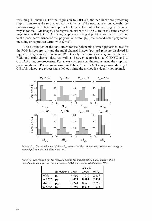
94

remaining 11 channels. For the regression to CIELAB, the non-linear pre-processing step still improves the results, especially in terms of the maximum errors. Clearly, the pre-processing step plays an important role even for multi-channel images, the same way as for the RGB-images. The regression errors to CIEXYZ are in the same order of magnitude as that to CIELAB using the pre-processing step. Attention needs to be paid to the poor performance of the polynomial vector pm4, the second-order polynomial including cross product terms, with Q = 37.

The distribution of the ∆Eab errors for the polynomials which performed best for the RGB images (p2, p3) and the multi-channel images (pm2 and pm5) are displayed in Fig. 7.2, using standard illuminant D65. Clearly, the results are very similar between RGB and multi-channel data, as well as between regressions to CIEXYZ and to CIELAB using pre-processing. For an easy comparison, the results using the 4 optimal polynomials and D65 are summarized in Tables 7.5 and 7.6. The regression directly to CIELAB without pre-processing is left out, since the method is evidently not optimal.

Figure 7.2. The distribution of the ∆Eab errors for the colorimetric estimations, using the optimal polynomials and illuminant D65.

Table 7.5. The results from the regression using the optimal polynomials, in terms of the Euclidian distance in CIEXYZ color space, ∆XYZ, using standard illuminant D65.

Regression

Max

∆XYZMean

95%

p2 4.900 1.019 2.488 RGB to XYZ p3 3.453 0.904 2.151

pm2 3.240 0.945 2.399 Multi to XYZ pm5 3.759 0.932 1.732

0 50

20

40

60

∆Eab

Sam

ples

(%

)

P2, XYZ

0 50

20

40

60

∆Eab

P3, XYZ

0 50

20

40

60

∆Eab

Pm2

, XYZ

0 50

20

40

60

∆Eab

Pm5

, XYZ

0 50

20

40

60

∆Eab

Sam

ples

(%

)

P2, Lab

0 50

20

40

60

∆Eab

P3, Lab

0 50

20

40

60

∆Eab

Pm2

, Lab

0 50

20

40

60

∆Eab

Pm5

, Lab

95

Table 7.6. The results from the regression using the optimal polynomials, in terms of CIE 1976 color difference ∆Eab and CIE 1994 color difference ∆E94, using standard illuminant D65.

Regression

Max

∆Eab Mean

95%

Max

∆E94 Mean

95%

p2 4.293 1.942 3.222 2.519 1.230 2.007 RGB to XYZ p3 4.558 2.086 3.948 2.620 1.184 2.450

pm2 3.765 1.942 3.227 2.245 1.162 2.130 Multi to XYZ pm5 3.164 1.962 3.131 2.913 1.234 2.318

p2 3.637 1.762 3.066 3.089 1.176 2.150 RGB1/3 to Lab p3 4.317 1.722 3.368 3.046 1.113 1.996

pm2 3.846 1.957 3.786 2.417 1.221 1.981 Multi1/3 to Lab pm5 3.250 1.774 2.810 2.280 1.213 2.138

Reducing the training set To investigate the influence of the number of color samples in the training set used to derive the characterization function, we perform the same experiments using only 25 of the 50 test colors. The results for the polynomials giving the best result for RGB and multi-channel images, i.e. p2, p3, pm2 and pm5, are given in Tables 7.7 and 7.8 The results are computed using the standard illuminant D65 and should be compared to the results in Tables 7.5 and 7.6.

Table 7.7. The results when reducing the training set to 25 test colors, in terms of the Euclidian distance in CIEXYZ color space, ∆XYZ, using standard illuminant D65.

Regression

Max

∆XYZMean

95%

p2 5.712 1.137 2.760 RGB to XYZ p3 5.916 1.785 4.576

pm2 5.788 1.136 2.436 Multi to XYZ pm5 8.261 2.272 4.987

Table 7.8. The results when reducing the training set to 25 test colors, in terms of CIE 1976 color difference ∆Eab and CIE 1994 color difference ∆E94, using standard illuminant D65.

Regression

Max

∆Eab Mean

95%

Max

∆E94 Mean

95%

p2 5.242 2.579 5.092 4.282 1.523 2.827 RGB to XYZ p3 20.70 4.132 10.11 14.53 2.495 5.375

pm2 6.216 2.456 4.372 2.918 1.375 2.401 Multi to XYZ pm5 11.39 5.721 11.17 8.999 3.485 7.908

p2 5.551 2.207 4.612 3.091 1.273 2.547 RGB1/3 to Lab p3 6.210 2.792 5.532 5.094 1.896 3.575

pm2 8.251 3.301 6.730 5.182 2.197 4.130 Multi1/3 to Lab pm5 15.18 4.086 8.828 11.07 2.782 6.450

As could be expected the errors increases when the training set is reduced by half. It is clear that the more terms included in the polynomials, the larger the increase of estimation errors. For example, for RGB-images, p2 (Q=11) now clearly outperforms p3

96

(Q=20). Similarly, for the multi-channel images, pm2 (Q=16) performs better than pm5 (Q=22). This is because higher order polynomials including more polynomial terms, need larger training sets for optimal performance. The best performance is obtained for the second order polynomial p2, using regression from RGB to CIELAB with the pre-processing step. It should be noted that 25 color samples included in the training set is still sufficient for the system of equations to be over determined, for the polynomials in question.

The mean and maximal estimation errors in terms of ∆Eab when varying the number of training colors included in the training set from 50 to 20, are given in Appendix C. The results further verifies that the simpler polynomials are more robust when decreasing the training set.

Cross-media characterization Experiments on cross-media characterization is performed to investigate to what extent the characterization is affected by eye-camera metamerism, i.e. how the derived functions perform when using color samples of different media and colorants. Tables 7.9 and 7.10 collect the results when using the characterization functions derived for the printed color patches, to estimate colorimetric data for NCS colors. Observe that the color of the NCS patches are created using different pigments, therefore have very different characteristics compared to the printed color patches of the training set.

Table 7.9. The results for cross-media characterization, in terms of the Euclidian distance in CIEXYZ color space, ∆XYZ, using standard illuminant D65.

Method

Max

∆XYZMean

95%

p2 24.95 13.06 22.13 RGB to XYZ p3 25.55 12.96 21.12

Linear 10.46 4.176 9.246 pm2 13.71 5.366 11.07

Multi to XYZ

pm5 23.88 16.15 23.19

Table 7.10. The results for cross-media characterization, in terms of CIE 1976 color difference ∆Eab and CIE 1994 color difference ∆E94, using standard illuminant D65.

Method

Max

∆Eab Mean

95%

Max

∆E94 Mean

95%

p2 58.59 11.31 31.35 19.50 7.309 14.70 RGB to XYZ p3 16.67 9.494 16.29 13.43 7.437 11.33

Linear (7) 27.76 4.850 9.636 15.68 3.256 5.840 pm5 26.00 9.781 22.21 15.04 6.316 11.95

Multi to XYZ

pm2 40.28 18.14 37.66 25.90 10.18 22.12 P2 18.29 8.417 14.66 11.66 6.821 10.48 RGB1/3

to Lab P3 27.27 10.51 22.60 20.67 7.984 16.66 Linear (7) 18.76 8.877 17.85 15.30 5.945 12.41 Multi1/3

to Lab pm5 63.31 22.78 54.25 27.23 13.51 26.37 pm2 80.98 20.55 61.35 36.64 12.06 27.14

97

It is evident from the results that the eye-camera metamerism is severe. The estimation errors increases dramatically, regardless which metrics is used to evaluate the result. For the polynomial regressions, the RGB-images give better performance than the multi-channel images. The best result is actually obtained using the basic linear regression from multi-channel data to CIEXYZ. It is evident from the result that direct polynomial regression is optimized only for the specific combination of media and colorant used to derive the characterization function. It seems that the more complex the estimation function, i.e. the order of the polynomial and the number of terms included, the stronger the effect of the cross media characterization.

7.5.2 Spectral regression

The spectral reconstruction matrix A has been derived according to Eq. 7.2, using the recorded device response for the set of 50 training colors. To be directly comparable with the results from the model-based characterization, the spectral reflectance is estimated in the range 400:4:700 nm, giving N = 76, i.e. N >T and the system is thus underdetermined.

The spectral reflectance has been reconstructed according to Equation 7.3, for the set of 50 evaluation colors. As before, we can utilize the a priori knowledge that spectral reflectance are typically smooth functions, to represent the reconstructed spectra as linear combinations of smooth basis functions. As with the model-based approach, we evaluate spectral basis, using the NCS database, as well as Fourier basis. Five basis functions are used, corresponding to the first five Fourier basis functions and to the five singular vectors corresponding to the most significant singular values in the spectral autocorrelation function of the spectral database.

The results from the empirical spectral reconstruction, in terms of spectral RMS difference and ∆XYZ are given in Table 7.11. The corresponding colorimetric reconstruction errors in terms of CIE color differences, ∆Eab and ∆E94, are listed in Tab. 7.12, computed using D65. Examples of estimated spectral reflectance for 3 different color samples are presented in Figs 7.3 and 7.4, derived from RGB and multi-channel images, respectively.

Table 7.11. Spectral reconstruction errors, expressed as RMS difference in spectral space, and the Euclidian distance in CIEXYZ space, ∆XYZ.

Data

Method

Max

RMS Mean

95%

Max

∆XYZ Mean

95%

PI 0.0082 0.0023 0.0050 10.64 4.884 9.937 Spectral 0.0062 0.0031 0.0057 10.15 5.090 9.988

RGB

Fourier 0.0072 0.0035 0.0064 10.13 5.017 9.714 PI 0.0030 0.0004 0.0013 8.496 2.301 6.284 Spectral 0.0040 0.0018 0.0036 8.396 2.891 7.882

Multi

Fourier 0.0052 0.0023 0.0044 7.678 2.531 6.490

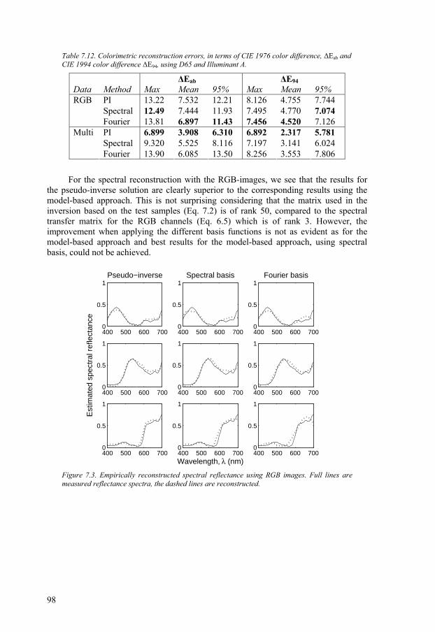
98

Table 7.12. Colorimetric reconstruction errors, in terms of CIE 1976 color difference, ∆Eab and CIE 1994 color difference ∆E94, using D65 and Illuminant A.

Data

Method

Max

∆Eab Mean

95%

Max

∆E94 Mean

95%

PI 13.22 7.532 12.21 8.126 4.755 7.744 Spectral 12.49 7.444 11.93 7.495 4.770 7.074

RGB

Fourier 13.81 6.897 11.43 7.456 4.520 7.126 PI 6.899 3.908 6.310 6.892 2.317 5.781 Spectral 9.320 5.525 8.116 7.197 3.141 6.024

Multi

Fourier 13.90 6.085 13.50 8.256 3.553 7.806

For the spectral reconstruction with the RGB-images, we see that the results for the pseudo-inverse solution are clearly superior to the corresponding results using the model-based approach. This is not surprising considering that the matrix used in the inversion based on the test samples (Eq. 7.2) is of rank 50, compared to the spectral transfer matrix for the RGB channels (Eq. 6.5) which is of rank 3. However, the improvement when applying the different basis functions is not as evident as for the model-based approach and best results for the model-based approach, using spectral basis, could not be achieved.

Figure 7.3. Empirically reconstructed spectral reflectance using RGB images. Full lines are measured reflectance spectra, the dashed lines are reconstructed.

400 500 600 7000

0.5

1Pseudo−inverse

400 500 600 7000

0.5

1Spectral basis

400 500 600 7000

0.5

1Fourier basis

400 500 600 7000

0.5

1

Est

imat

ed s

pect

ral r

efle

ctan

ce

400 500 600 7000

0.5

1

400 500 600 7000

0.5

1

400 500 600 7000

0.5

1

400 500 600 7000

0.5

1

Wavelength, λ (nm)400 500 600 7000

0.5

1

99

Figure 7.4. Empirically reconstructed spectral reflectance using multi-channel images. Full lines are measured reflectance spectra, the dashed lines are reconstructed.

The results of the spectral reconstruction improve for multi-channel images compared to RGB-images, but not to the same degree as the corresponding improvement achieved for the model-based approach. In terms of spectral RMS difference, the results are comparable to the model-based results (compare to Tab. 6.1). However, in terms of colorimetric differences, the estimation errors are always larger. The best results obtained, in terms of ∆Eab color difference, were for the PI method, which under the illuminant D65 produced estimates with a mean color difference of 3.9 ∆Eab and the maximum 6.9 ∆Eab. This is to be compared to the corresponding results for the model based approach, giving a mean color difference of 1.5 ∆Eab and the maximum 4.4 ∆Eab (Tab. 6.2).

Histograms of the distribution of the CIE 1976 ∆Eab, differences using D65 are given in Fig. 7.5, for the different reconstruction methods. The results improve for multi-channel images, but not to the same levels of accuracy obtained using the model-based approach (compare to Fig. 6.3). Restricting the reconstructed spectra to be linear combinations of basis functions does not improve the result for the multi-channel images.

If the aim is to estimate colorimetric data only, the polynomial regression directly to CIEXYZ and CIELAB are clearly superior to computing colorimetric values from the empirical spectral reconstructions (compare to Tables 7.5 and 7.6, Fig. 7.2). At least, this is true for samples of the same media and colorant that has been used to derive the characterization function.

400 500 600 7000

0.5

1Pseudo−inverse

400 500 600 7000

0.5

1Spectral basis

400 500 600 7000

0.5

1Fourier basis

400 500 600 7000

0.5

1

Est

imat

ed s

pect

ral r

efle

ctan

ce

400 500 600 7000

0.5

1

400 500 600 7000

0.5

1

400 500 600 7000

0.5

1

400 500 600 7000

0.5

1

Wavelength, λ (nm)400 500 600 7000

0.5

1

100

Figure 7.5. The distribution of the ∆Eab errors between measured and reconstructed spectral reflectance, using empirical spectral reconstruction. Standard illuminant D65.

Cross media characterization To investigate how the empirical spectral reconstruction performs when used to reconstruct spectral reflectance for color samples of different media and colorants, we perform experiments on cross-media characterization. In the following, the spectral reconstruction matrix derived for the printed training set, has been used to reconstruct spectral reflection for the set of NCS color patches.

The results from the cross-media spectral reconstruction are given in Tables 7.13 and 7.14, using D65. Examples of estimated spectral reflectance using RGB and multi-channel data are presented in Appendix C.

Table 7.13. Spectral reconstruction errors for cross-media characterization, expressed as RMS difference in spectral space, and the Euclidian distance in CIEXYZ space, ∆XYZ.

Data

Method

Max

RMS Mean

95%

Max

∆XYZ Mean

95%

PI 0.0245 0.0076 0.0223 24.68 10.78 20.27 Spectral 0.0238 0.0069 0.0221 24.65 11.58 21.61

RGB

Fourier 0.0215 0.0067 0.0183 23.22 11.01 20.87 PI 0.0187 0.0024 0.0058 11.02 4.247 9.610 Spectral 0.0151 0.0016 0.0038 12.86 4.792 9.955

Multi

Fourier 0.0134 0.0022 0.0052 13.66 5.498 10.78

0 5 10 150

10

20

∆Eab

Sam

ples

(%

)

RGBPseudo−inverse

0 5 10 150

10

20

∆Eab

RGBSpectral basis

0 5 10 150

10

20

∆Eab

RGBFourier basis

0 5 10 150

10

20

∆Eab

Sam

ples

(%

)

MultiPseudo−inverse

0 5 10 150

10

20

∆Eab

MultiSpectral basis

0 5 10 150

10

20

∆Eab

MultiFourier basis

101

Table 7.14. Spectral reconstruction errors for cross-media characterization, in terms of CIE 1976 color difference, ∆Eab and CIE 1994 color difference ∆E94, using D65.

Data

Method

Max

∆Eab Mean

95%

Max

∆E94 Mean

95%

PI 43.25 9.237 20.25 20.42 6.084 9.309 Spectral 41.42 8.807 19.33 21.45 6.105 9.638

RGB

Fourier 26.20 7.509 12.84 17.44 5.732 8.807 PI 22.55 4.662 9.703 14.63 3.201 5.813 Spectral 16.44 3.666 7.817 11.27 2.755 4.609

Multi

Fourier 24.53 5.354 15.10 14.29 3.300 5.320

Clearly, the reconstruction errors increase for the cross-media applications (compare to Tables 7.11 and 7.12), especially in terms of the maximal errors. When the reconstruction matrix is used for other media and colorants, the improvement using multi-channel data compared to RGB-data is more obvious. The pseudo-inverse method, which provided the best results reconstructing spectral reflectance for the same media and colorant, is now clearly outperformed by the methods using base functions. Fourier basis give the best results for RGB-data, while the spectral basis give the best results for multi-channel data. Notice that the spectral basis is computed from the NCS spectral data base, which should have the advantage when used to reconstruct reflectance spectra of other NCS color patches. The best results for the cross-media characterization are obtained using multi-channel data and spectral basis, giving mean errors comparable to the results using the same media and colorants, but with the maximal errors more than doubled.

Note that, when compared to the results for cross-media characterization using direct regression to CIEXYZ and CIELAB (Tables 7.9 and 7.10), the estimation errors decreases when the colorimetric data is computed from the reconstructed spectra. This is probably due to the fact that the eye-camera metamerism is avoided when the regression is used to estimate spectral reflectance. Even though the spectral reconstruction method could not compete with the direct colorimetric regression to estimate colorimetric data using the same media and colorant, it is clearly more robust when estimating colorimetric values for color samples of different-media and colorants.

7.6 Summary and discussion In this chapter, empirical characterization has been used to derive mappings from device dependent data to the colorimetric representations CIEXYZ and CIELAB, and to reconstruct spectral reflectance from the recorded device signals. In the empirical approach, the spectral characteristics of the system are ignored and the mappings are derived by relating the recorded device response for a set of training colors, using least squares regression techniques. The main drawback is that the characterization will be optimized only for the specific set of conditions, including the colorant and the media, used to derive the characterization functions.

The results for the empirical characterization showed that a good colorimetric accuracy could be obtained by using polynomial regression to the colorimetric representations CIEXYZ and CIELAB. The results for RGB-images were equally good as for the multi-channel images, and offered the same colorimetric accuracy as for the

102

model-based characterization using multi-channel images. However, the accuracy is dependent on that the mappings are derived using the same media and colorant. Experiments on cross-media characterization revealed that the eye-camera metamerism is severe, producing large errors when the characterization functions are used for different media and colorants.

Empirical techniques were also used to reconstruct spectral reflectance, by deriving a spectral reconstruction matrix based on measurements on the training set. The results revealed that for RGB-images, the pseudo-inverse method performed considerably better than the corresponding model-based approach. However, using multi-channel images and building the spectra from basis functions did not improve the results to the same degree, and the level of accuracy obtained for the model-based approach could not be reached for the empirical spectral estimations.

The spectral reconstruction using regression could possibly be improved by increasing the training set used to derive the reconstruction matrix. Alternatively, the spectra could be reconstructed using a coarser interval, e.g. 400:10:700 nm, giving N = 31, and thus a reconstruction matrix of sufficient rank. However, the empirical approach will still suffer from the media dependence, making the more general model-based approach a better choice, at least when multi-channel data is available.

103

Chapter 8 8 Summary and future work

Summary and future work

8.1 Summary 8.2 Future work

104

105

8.1 Summary The focus of this thesis has been on acquisition of colorimetric and multispectral images. To ensure stability and repeatability, a thorough calibration of the system has been carried out, to gain understanding on the performance of all components, and how they meet their respective demands. The spectral image acquisition model, describing the device response to a known spectral input, has been derived, including the spectral characteristics of the illumination, the color filters and the CCD camera.

The spectral sensitivity function for the camera, combining the spectral transmittance of the optics and the quantum efficiency of the CCD, which could not be obtained by direct measurements, has been estimated. By relating measured reflectance spectra to the corresponding device responses, for a set of carefully selected training colors, the sensitivity function was derived using least square regression. The principle eigenvector method was used to reduce the noise sensitivity, and a priori knowledge on the nature of camera sensitivity was used as constraints in the regression. The estimated sensitivity function was similar to the function derived from the manufacturer data, but reduced the prediction errors by more than half.

To reconstruct colorimetric and spectral data from the recorded device response, two conceptually different characterization methods have been investigated: model-based and empirical characterization. In the model-based approach, the spectral model of the image acquisition is inverted, to reconstruct the spectral reflectance of objects from the recorded device responses. A priori knowledge on the smooth nature of spectral reflectance was utilized by representing the reconstructed spectra as linear combinations of basis functions, using Fourier basis and a set of real reflectance spectra.

The results showed that a satisfactory spectral or colorimetric accuracy could not be obtained from trichromatic images. When using multi-channel images, the improvement was significant, both in terms of colorimetric differences and in the RMS spectral reconstruction error. The best overall performance was obtained by the method using spectral basis. However, if the aim is only to derive colorimetric data, the simple pseudo-inverse method is sufficient, producing reconstructions that are good metameric matches.

In the empirical approach, the spectral characteristics of the system are ignored and the mappings are derived by relating the recorded device response to colorimetric and spectral data for a set of training colors, using least squares regression techniques.

106

The main drawback is that the characterization will be optimized only for the specific set of conditions, including the colorant and the media, used to derive the characterization functions.

Empirical characterization was used to derive mappings to the colorimetric representations of CIEXYZ and CIELAB, and to reconstruct spectral reflectance. The results showed that a good colorimetric accuracy could be obtained by using polynomial regression to CIEXYZ and CIELAB. The results for trichromatic images were equally as good as for the multi-channel images, and offered the same colorimetric accuracy as for the model-based approach, using multi-channel images. However, experiments on cross-media characterization revealed that the accuracy is limited to the case when the mappings are used for the same media and colorant from which they are derived.

The results when using empirical techniques to reconstruct spectral reflectance revealed that, for trichromatic images, the performance was comparable to the trichromatic model-based results. However, for multi-channel images the level of accuracy obtained for the model-based approach could not be reached, using empirical spectral reconstruction.

To conclude, the results have showed that in the cases when only trichromatic imaging is available, the best method for colorimetric imaging is the empirical approach, using polynomial regression. However, because of the media-dependency, this requires for the characterization functions to be derived for each combination of media and colorants. For multispectral imaging, reconstructing the spectral reflectance of objects, multi-channel images are required to obtain the highest accuracy. The best results were obtained with the model-based approach and multi-channel images, combined with spectral basis. The model-based approach provides the additional advantage of being general, since it is based on the spectral characteristics of the image acquisition system, not on the characteristics of a set of color samples. The accuracy achieved in the model-based characterization also indicates that the image acquisition model is accurate, reflecting the real characteristics of the image acquisition system well.

8.2 Future work This work has focused on the image acquisition system, obtaining knowledge of all components, and deriving methods to reconstruct colorimetric and spectral data. These results form the necessary basis for the continuation, which naturally is to use the system for high quality colorimetric and multispectral image acquisition.

The image acquisition system has primarily been designed for acquiring macro images of prints and substrates, with the main purpose of studying micro-scale properties of prints. We believe that studying color prints on a micro-scale level offers news way to characterize different properties associated with color printing (Nyström & Kruse, 2005; Nyström, 2005). Hopefully the ideas can be further developed to gain a deeper understanding and possibly to improve models dealing with color reproduction of printing.

The flexibility of the image acquisition system, such as varying the angle of incident illumination, and backlight for transmission imaging, opens up many possibilities for different experiments. The knowledge of the system and the high level of spectral and colorimetric accuracy, gained in this work, will be of great importance

107

for future works. We believe that the possibility to accurately estimate the spectral reflectance in each pixel of high resolution images will open up many possibilities in our future research with the focus on print color reproduction.

108

109

Bibliography

Ajito, Takeyuki, et al. (2000). Expanded color gamut reproduced by six-primary projection display. Proc. SPIE: Projection Displays 2000, Vol. 3954, pp 130-137.

Andersson, Mattias, et al. (2003). The Substrate influence on color measurement, Proc. IS&T NIP 19, New Orleans, 2003.

Andersson, Mattias (2004). Color measurements using Digital Cameras, Proc. IPGAC04 Conference, Vancouver, 2004.

Andersson, Mattias (2006). Colour Calibration of Trichromatic Capturing Devices. Ph.D. thesis, dissertation No. 1059, Linköping University, 2006.

Bala, Raja (2003). Device characterization. In Sharma, Gaurav (editor) Digital Color Imaging Handbook, CRC Press LLC, 2003.

Barnard, Kobus & Funt, Brian (2002). Camera Characterization for Color Research, in COLOR research and application, volume 27, number 3, June 2002.

Berns, Roy S. et al. (1998) Multi-spectral-based color reproduction research at the Munsell Color Science Laboratory. In Electronic Imaging: Processing, Printing, and Publishing in Color, Proc. SPIE Vol. 3409, 1998, pp 14-25.

Cheung, Vien et al. (2005) Characterization of trichromatic color cameras by using a new multispectral imaging technique. In J. Opt. Soc. Am. A, Volume 22, No. 7, July 2005, pp 1231-1240.

CIE (1995). Industrial Color-Difference Evaluation. CIE publication No. 116, CIE Central Bureau, Vienna, 1995.

CIE (2001). Improvement to industrial Color-Difference Evaluation. CIE publication No. 142, CIE Central Bureau, Vienna, 2001.

Connah, D. et al (2001). Recovering spectral information using digital camera systems. In Coloration technology, vol 117, 2001, pp 309-312.

DiCarlo, Jeffrey M. et al. (2004). Emissive Chart for Imager Calibration. Proc. The Twelfth Color Imaging Conference: Color Science, Systems and Applications, pp. 295-301, 2004.

110

E2V technologies (2003). Technical notes on the MTF of CCD Sensors. A1A-CCTN105 Issue 5, June 2003.

Fairchild, Mark D. (1998). Color Appearance Models. Second Edition. Addison Wesley, 1998. ISBN 0-201-63464-3.

Fairchild, Mark D. et al. (2001). Spectral and Metameric Color Imaging. Technical Report, Munsell Color Science Laboratory, August 2001.

Farell, J.E, et al. (1999), Estimating Spectral Reflectances of Digital Artwork. Proc. Chiba Conference of Multispectral Imaging, 1999.

Field, Gary G (1999). Color and Its Reproduction. Second Edition. GATFPress, ISBN 0-88362-201-7.

Finlayson, Graham D. & Hubel, Paul M. (1998). Recovering Device Sensitivities with Quadratic Programming. Proc. The Sixth Color Imaging Conference: Color Science, Systems and Applications, pp. 90-95, 1998.

Haneishi, H, et al. (2000). System design for accurately estimating the spectral reflectance of art paintings. In Applied Optics Vol. 39, No. 35, pp.6621-6632.

Hardeberg, Jon Yngve (2001) Acquisition and Reproduction of Color Images: Colorimetric and Multispectral Approaches, Dissertation.com, 2001, ISBN 1-58112-135-0.

Hess, C. (2002). Multifunctional Target for the Analysis of optical characteristics of Low and High Magnification systems, Max Levy Autograph, Inc, 2002.

Hill, Bernhard (1999). Color capture, color management, and the problem of metamerism: does multispectral imaging offer the solution? Proc. SPIE: Color Imaging: Device-Independent Color, Color Hardcopy, and Graphic Arts V, Vol. 3963, 1999, pp. 2-14.

Hong, Gouwei & Lou, M. R. (2000). A Study of Digital Camera Colorimetric Characterization Based on Polynomial Modeling. In COLOR research and application, volume 26, Number 1, February 2001.

Hunt, R.W.G (1995). The Reproduction of Colour, Fifth Edition, Kingston-upon-Thames, Fountain Press, ISBN 0 86343 381 2.

Hunt, R.W.G (1998). Measuring Colour, Third Edition, Kingston-upon-Thames, Fountain Press, ISBN 0 86343 387 1.

Hård, Anders (1995). Färgantologi bok 1, Färgsystemet NCS: tanke, tillkomst, tillämpning. Statens råd för byggforskning, Stockholm, 1995, ISBN 9154056942.

ICC (2004). Specification ICC.1:2004-10 (Profile version 4.2.0.0) Image technology colour management — Architecture, profile format, and data structure.

Imai, Francisco H, & Berns, Roy S. (1999). Spectral Estimation Using Trichromatic Digital Cameras. Proc. International Symposium on Multispectral Imaging and Color Reproduction for Digital Archives, Chiba, 1999, pp 42-49.

Imai, Francisco H, et al. (2000). Comparison of Spectrally Narrow-Band Capture Versus Wide-Band with a priori Sample Analysis for Spectral Reflectance Estimation. Proc. IS&T/SID Eight Color Imaging Conference, 2000, pp. 234-241.

111

Imai, Francisco H, et al. (2001a). Digital camera filter design for colorimetric and spectral accuracy. Proc. 3rd International Conference on Multispectral Color Science, 2001, pp 23-26.

Imai, Francisco H, et al. (2001b). Spectral reproduction from scene to hardcopy: I. Input and output. Proc. IS&T/SPIE Conference on Color Imaging: Sensors and Camera Systems for Scientific, Industrial and Digital Photography Applications II, 2001, pp 346-357.

Imai, Francisco H, et al. (2002). Comparative Study of Metrics for Spectral Match Quality. Proc. CGIV 2002: The First European Conference on Colour Graphics, Imaging and Vision, pp. 492-496.

Kaiser, P.K. and Boynton, R.M (1996). Human Colour Vision, Second Edition, Optical Society of America, Washington, D.C., 1996.

Kipphan, Helmut (2001). Handbook of Print Media. Springer-Verlag, 2001, ISBN 3-540-67326-1.

Kraushaar, Andreas & Urban, Philipp (2006). How to linearise a multispectral printing system for graphic arts uses? In Advances in Printing Science and Technology, Volume 33, 2006.

Lou, M.R, et al. (2001). The Development of the CIE 2000 Colour-Difference Formula: CIEDE2000. In Colour Research and Application, Volume 26, Issue 5, pp 340-350, 2001.

Maloney, L.T. (1986). Evaluation of linear models of surface spectral reflectance with small numbers of parameters. In J. Opt. Soc. Am. A, 3, 1986.

Melgosa, Manuel, et al. (2004). Relative significance of the terms in the CIEDE2000 and CIE94 color-difference formulas. In J. Opt. Soc. Am. A, Volume 21, Issue 12, pp 2269-2275.

Martínez-Verdú, Francisco, et al. (2000). Calculation of the Color-Matching Functions of Digital Cameras from their Complete Spectral Responsitivities. Proc. Eighth Color Imaging Conference: Color Science and Engineering Systems, Technologies, Applications, 2000, pp. 211-216.

Nyström, Daniel (2003). Hi-Fi Soft Proofing Using DLP. Proc. Technical Association of the Graphic Arts, Montreal, 2003, pp 197-146.

Nyström, Daniel & Kruse, Björn (2005). High resolution properties of color prints. Proc. CSIST/IS&T Beijing International Conference on Imaging, 2005, pp 242-243.

Nyström, Daniel (2005). Micro-scale properties of color prints. Proc. Printing Future Days, Chemnitz, 2005, pp 154-158.

Nyström, Daniel & Kruse, Björn (2005). Colorimetric Device Characterization for Accurate Color Image Acquisition. In Advances in Printing and Media Technology, Vol. 33, 2006.

Pan, Zhihong, et al. (2001). Color Scanner Characterization with Scan Targets of Different Media Types and Printing Mechanisms. Proc. Color Imaging: Device-Independent Color, Color Hardcopy, and Graphic Arts VI, 2001, pp 58-63.

112

Parulski, Ken & Spaulding, Kevin (2003). Color image processing for digital cameras. In Sharma, Gaurav (editor) Digital Color Imaging Handbook, CRC Press LLC, 2003.

Pauler, Nils (1998). Paper Optics. AB Lorentzen & Wettre, Sweden.

PCO Imaging (2003). PixelFly Operating Instructions. Version 05, 2003.

Photo Research (1999). PR-650 SpectraScan® SpectracolorimeterTM Instruction Manual, Document # 9903-0006-05 Rev. B, 1999.

Quan, Shuxue (2002). Evaluation and Optimal Design of Spectral Sensitivities for Digital Color Imaging. Ph.D. Thesis, Center for Imaging Science, Rochester Institute of Technology.

Rosen, Mitchell R. et al. (2000). Color Management within a Spectral Image Visualization Tool. Proc. IS&T/SID Eight Color Imaging Conference, 2000, pp. 75-80.

Rosen, Mitchell R. et al. (2001). Spectral reproduction from scene to hardcopy: II. Image processing. Proc. SPIE Color Imaging: Device-Independent Color, Color Hardcopy, and Graphic Arts VI, Vol. 4300, pp. 33-41.

Rydefalk, Staffan & Wedin, Mikael (1997). Literature Review on the Colour Gamut in the Printing Process. PFT rapport nr 32. PFT, 1997.

Schott-Fostech, LLC (2002) DCR® III –Direct Current Regulated Light Source – Users Manual and Technical Reference, 2002.

Sharma, Guarav (2003). Color fundamentals for digital imaging. In Sharma, Gaurav (editor) Digital Color Imaging Handbook. CRC Press LLC.

Sharma, Gaurav & Trussell, H. J. (1996). Set theoretic estimation in color scanner characterization. In J. Electronic Imaging, 5(4), pp. 479-489.

Schneider Kreuznach (2004). Macro System, Ident.-Nr.: 27887, [www] <www.schneideroptics.com> (available 2006-03-08).

Solli, Martin (2004). Filter characterization in digital cameras. Master thesis, Institute of Science and Technology, Linköping University, 2004.

Solli, Martin, et al. (2005). Color Measurements with a Consumer Digital Camera Using Spectral Estimation Techniques. Proc. Scandinavian Conference on Image Analysis, 2005.

Sugiura, H. et al. (1999). Development of Highly Accurate Multispectral Cameras. Proc. International Symposium on Multispectral Imaging and Color Reproduction for Digital Archives, 1999, pp 79-80.

Susstrunk, Sabine, et al. (1999) Standard RGB Color Spaces, Proc. IS&T/SID Seventh Color Imaging Conference: Color Science, Systems and Applications, 1999, pp 127-134.

Trussel, H. Joel, et al. (2005). Color image processing [basics and special issue overview]. In IEEE Signal Processing Magazine, volume 22, pp 14-22, Jan 2005.

Tzen, Di-Yuan & Berns, Roy S. (2000). Spectral-Based Six-Color Separation Minimizing Metamerism. Proc. IS&T/SID Eight Color Imaging Conference, 2000, pp. 342-347.

113

VanWalree, Paul (2006). Vignetting. [www] <www.pinnipedia.org/optics> (available 2006-11-08).

Willert, Andreas, et al. (2006). Spectral-based colour reproduction workflow. In Advances in Printing Science and Technology, Volume 33, 2006.

Wyszecki, G., and Stiles, W.S (2000). Color science: concepts and methods, quantitative data and formulae, Second Edition, John Wiley and Sons, New York, 2000.

Yamaguchi, Masahiro, et al. (2001). Color image reproduction based on the multispectral and multiprimary imaging: experimental evaluation. Proc. SPIE: Color Imaging: Device-Independent Color, Color Hardcopy, and Applications VII, Vol. 4663, 2001, pp 15-26.

114

115

Appendices Appendices

A Device calibration data B Spectral sensitivity estimation data C Empirical characterization data

116

117

Appendix A: Device calibration data Appendix A contains data and results from the calibration of the image acquisition system, described in Chapter 4.

Illumination

Figure A.1 displays the total radiant power at different lamp intensity levels. Normalized spectral power distributions for different lamp intensity levels, from 10% to 100% are displayed in Fig. A.2. For clarity, when comparing the spectral properties of the lamp at different intensity levels, the spectral power distributions have all been normalized with respect to their maximum.

Figure A.1. The relation between measured radiant power and lamp intensity level.

0 20 40 60 80 1000

0.1

0.2

0.3

0.4

0.5

0.6

0.7

0.8

0.9

1

Lamp intensity (%)

Rel

ativ

e ra

dian

t pow

er

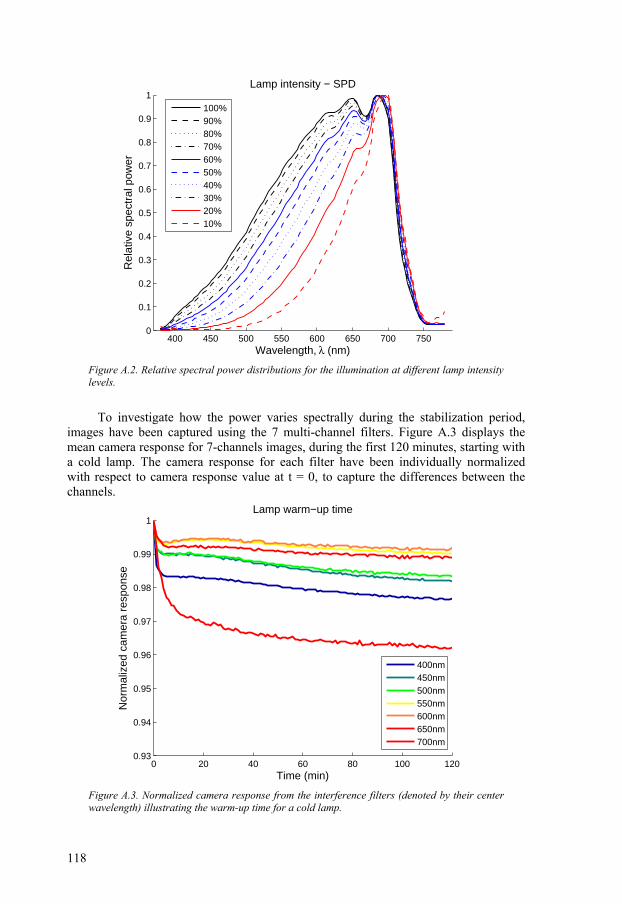
118

Figure A.2. Relative spectral power distributions for the illumination at different lamp intensity levels.

To investigate how the power varies spectrally during the stabilization period, images have been captured using the 7 multi-channel filters. Figure A.3 displays the mean camera response for 7-channels images, during the first 120 minutes, starting with a cold lamp. The camera response for each filter have been individually normalized with respect to camera response value at t = 0, to capture the differences between the channels.

Figure A.3. Normalized camera response from the interference filters (denoted by their center wavelength) illustrating the warm-up time for a cold lamp.

400 450 500 550 600 650 700 7500

0.1

0.2

0.3

0.4

0.5

0.6

0.7

0.8

0.9

1

Wavelength, λ (nm)

Rel

ativ

e sp

ectr

al p

ower

Lamp intensity − SPD

100%90%80%70%60%50%40%30%20%10%

0 20 40 60 80 100 1200.93

0.94

0.95

0.96

0.97

0.98

0.99

1

Time (min)

Nor

mal

ized

cam

era

resp

onse

Lamp warm−up time

400nm450nm500nm550nm600nm650nm700nm

119

As seen in Fig. A.3, the biggest variation occurs at the two ends of the visible spectrum, illustrated by the maximum decreases in wavelengths near the IR and UV, respectively. After about 30 minutes, the ratio of the camera response from the different channels is very close to constant, indicating that the power decreases uniformly over the visible spectrum. Since only the total power changes, the color information in the acquired images will be consistent, after this first stabilization period.

The spectral transmittance of the transmissive plate, Tp(λ), used for transmission images, is given in Fig. A.4

Figure A.4. Spectral transmittance for the transmissive plate.

Color filters

Figure A.5 displays the CIE xy-chromaticities of the RGB channels (including the illumination and the RGB filters). The white-point plotted corresponds to the case of equal exposure times, illustrating the lower energy for the blue channel. For comparison, the RGB chromaticities adopted in the sRGB standard are provided (Susstrunk et al., 1999). Clearly, the RGB chromaticities of the system differs some to sRGB (which is based on CRT phosphor properties), especially for blue and green. This not unexpected, nor is it a problem, since the purpose of the image acquisition system is not to capture images directly optimized for display on screen.

The corresponding xy-chromaticities for the 7 multi-channels are displayed in Fig. A.6. With these relatively narrow-banded filters, the chromaticities comes very close to the spectral locus and covers the majority of the visible colors, with the exception of the region of purest green

400 450 500 550 600 650 700 7500.1

0.2

0.3

0.4

0.5

0.6

0.7

0.8Transmissive plate

Wavelength, λ (nm)

Tra

nsm

ittan

ce

120

Figure A.5. CIE xy-chromaticities for the RGB channels (*), compared to the chromaticities according to the sRGB standard (x).

Figure A.6. CIE 1931 chromaticities for the interference filters.

0 0.2 0.4 0.6 0.80

0.1

0.2

0.3

0.4

0.5

0.6

0.7

0.8

0.9

x

y

CIE x,y chromaticity diagram

0 0.2 0.4 0.6 0.80

0.1

0.2

0.3

0.4

0.5

0.6

0.7

0.8

0.9

x

y

CIE x,y chromaticity diagram

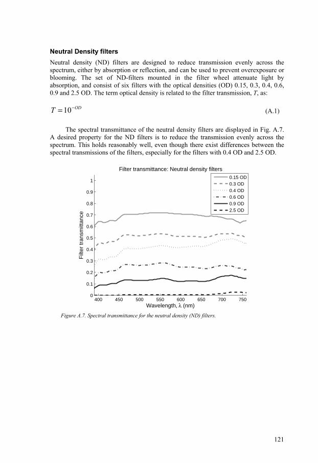
121

Neutral Density filters Neutral density (ND) filters are designed to reduce transmission evenly across the spectrum, either by absorption or reflection, and can be used to prevent overexposure or blooming. The set of ND-filters mounted in the filter wheel attenuate light by absorption, and consist of six filters with the optical densities (OD) 0.15, 0.3, 0.4, 0.6, 0.9 and 2.5 OD. The term optical density is related to the filter transmission, T, as:

ODT −= 10 (A.1)

The spectral transmittance of the neutral density filters are displayed in Fig. A.7. A desired property for the ND filters is to reduce the transmission evenly across the spectrum. This holds reasonably well, even though there exist differences between the spectral transmissions of the filters, especially for the filters with 0.4 OD and 2.5 OD.

Figure A.7. Spectral transmittance for the neutral density (ND) filters.

400 450 500 550 600 650 700 7500

0.1

0.2

0.3

0.4

0.5

0.6

0.7

0.8

0.9

1

Wavelength, λ (nm)

Filt

er tr

ansm

ittan

ce

Filter transmittance: Neutral density filters

0.15 OD0.3 OD0.4 OD0.6 OD0.9 OD2.5 OD

122

Polarization filter An additional polarization filter may optionally be used to reduce the influence of directed specular reflections in the images. The filter is an optical grade glass linear polarizing filter, and is attached directly to the optics. A linear polarizer transmits only light polarized in the same plane as the axis of the polarizer. The polarization axis can be varied by rotating the filter. The spectral transmittance of the polarization filter is displayed in Fig. A.8.

Figure A.8. The spectral transmittance for the polarization filter.

Optics

Figure A.9 gives the magnification curves for the optics, illustrating the relationship between the flange to image distance, the object-to-image distance and the magnification β. The magnification curves provide approximations of the resolution for different flange-to-image distances, and illustrate when the optics should be used in reverse position. The flange-to-image distance, from the mounting surface of the lens to the CCD-sensor, is given by the sum of the length of the extension rings, the back focal length of the lens (17.52 mm) and the camera C-Mount adapter (6.5 mm).

400 450 500 550 600 650 700 7500

0.05

0.1

0.15

0.2

0.25

0.3

0.35

0.4

0.45

0.5

Wavelength, λ (nm)

Filt

er tr

ansm

ittan

ce

Filter transmittance: Polarization filter

123

Figure A.9. The relationship between magnification ß’, flange-to-image distance and object-to-image distance (modified figure from Schneider Kreuznach, 2004).

Modulation Transfer Function, MTF The modulation transfer function, MTF, is a common measure of the ability of an optical system to resolve fine details (Hess, 2002). It is measured using test targets containing line patterns of varying spatial frequency. Such line patterns are called Ronchi Rulings and the spatial frequency is usually expressed in line pairs per mm (LP/mm). As the spatial frequency increases, the contrast decreases until that the details can no longer be resolved. The modulation is defined as:

minmax

minmax

LLLL

modulation+−

= (A.2)

where Lmax is the maximal luminance and Lmin is the minimum luminance. The modulation transfer function is then defined as the modulation of the image Mi at spatial frequency v, divided by the modulation of the stimulus, M0:

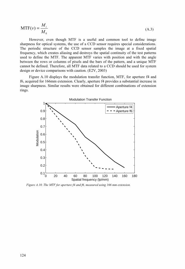
124

0

)(MTFMM

v i= (A.3)

However, even though MTF is a useful and common tool to define image sharpness for optical systems, the use of a CCD sensor requires special considerations. The periodic structure of the CCD sensor samples the image at a fixed spatial frequency, which creates aliasing and destroys the spatial continuity of the test patterns used to define the MTF. The apparent MTF varies with position and with the angle between the rows or columns of pixels and the bars of the pattern, and a unique MTF cannot be defined. Therefore, all MTF data related to a CCD should be used for system design or device comparisons with caution. (E2V, 2003)

Figure A.10 displays the modulation transfer function, MTF, for aperture f4 and f6, acquired for 166mm extension. Clearly, aperture f4 provides a substantial increase in image sharpness. Similar results were obtained for different combinations of extension rings.

Figure A.10. The MTF for aperture f4 and f6, measured using 166 mm extension.

0 20 40 60 80 100 120 140 160 1800.1

0.2

0.3

0.4

0.5

0.6

0.7

0.8

0.9

1

Spatial frequency (lp/mm)

Mod

ulat

ion

Modulation Transfer Function

Aperture f4Aperture f6

125

CCD camera

The mean values from a sequence of 50 images, captured using identical camera settings are displayed in Fig. A.11, to test for the repeatability of the CCD-sensor. The mean values from the series of images with varying integration times are displayed in Fig. A.12.

Figure A.11. The mean camera response from 50 sequentially captures images, for verification of CCD repeatability.

Figure A.12. Mean camera response for different exposure times, in the range 1:43 ms (top) and 10-440 ms (bottom) for verification of linearity with respect to integration time.

0 10 20 30 40 500.4

0.41

0.42

0.43

0.44

0.45

0.46

0.47

0.48

0.49

0.5

Images

Nor

naliz

ed c

amer

a re

spon

se (

mea

n)

CCD repeatability

0 10 20 30 40 500

0.2

0.4

0.6

0.8

1Integration time

0 50 100 150 200 250 300 350 4000

0.2

0.4

0.6

0.8

1

Exposure time (ms)

Nor

naliz

ed c

amer

a re

spon

se (

mea

n)

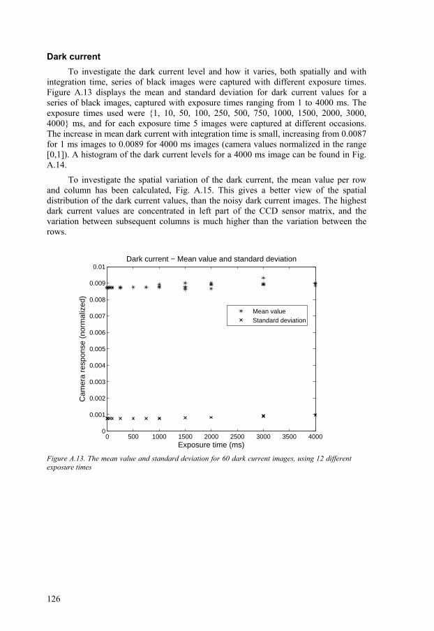
126

Dark current To investigate the dark current level and how it varies, both spatially and with

integration time, series of black images were captured with different exposure times. Figure A.13 displays the mean and standard deviation for dark current values for a series of black images, captured with exposure times ranging from 1 to 4000 ms. The exposure times used were {1, 10, 50, 100, 250, 500, 750, 1000, 1500, 2000, 3000, 4000} ms, and for each exposure time 5 images were captured at different occasions. The increase in mean dark current with integration time is small, increasing from 0.0087 for 1 ms images to 0.0089 for 4000 ms images (camera values normalized in the range [0,1]). A histogram of the dark current levels for a 4000 ms image can be found in Fig. A.14.

To investigate the spatial variation of the dark current, the mean value per row and column has been calculated, Fig. A.15. This gives a better view of the spatial distribution of the dark current values, than the noisy dark current images. The highest dark current values are concentrated in left part of the CCD sensor matrix, and the variation between subsequent columns is much higher than the variation between the rows.

Figure A.13. The mean value and standard deviation for 60 dark current images, using 12 different exposure times

0 500 1000 1500 2000 2500 3000 3500 40000

0.001

0.002

0.003

0.004

0.005

0.006

0.007

0.008

0.009

0.01

Exposure time (ms)

Cam

era

resp

onse

(no

rmal

ized

)

Dark current − Mean value and standard deviation

Mean valueStandard deviation

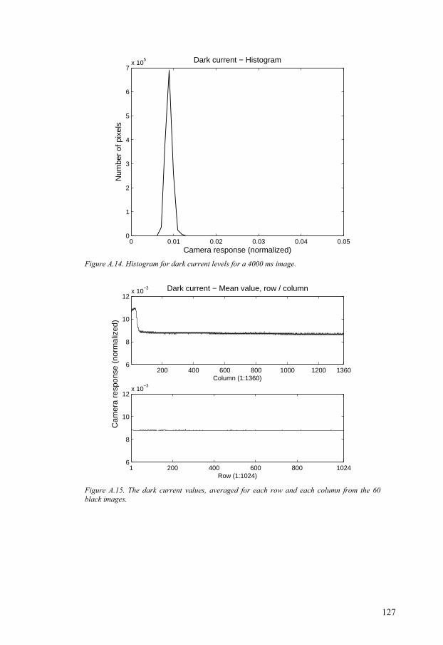
127

Figure A.14. Histogram for dark current levels for a 4000 ms image.

Figure A.15. The dark current values, averaged for each row and each column from the 60 black images.

0 0.01 0.02 0.03 0.04 0.050

1

2

3

4

5

6

7x 10

5

Camera response (normalized)

Num

ber

of p

ixel

s

Dark current − Histogram

200 400 600 800 1000 1200 13606

8

10

12x 10

−3 Dark current − Mean value, row / column

Column (1:1360)

1 200 400 600 800 10246

8

10

12x 10

−3

Row (1:1024)

Cam

era

resp

onse

(no

rmal

ized

)

128

129

Appendix B: Spectral sensitivity estimation data Appendix B contains data from the spectral sensitivity estimation, described in Chapter 5.

Table B.2 lists the 25 most spectrally varying NCS colors under the illuminant of the system, selected for the spectral sensitivity estimation according to Eqs 5.20-5.22.

Table B.1. The 25 NCS colors used for the spectral sensitivity estimation.

S2070R S0550Y50R S0570Y50R S0505R50B S1060Y000 S0570Y S3040R50B S1040B50G S2050Y S1080Y50R S0585Y50R S1050B000 S0540R S1040R S3005R50B S1040R50B S2040Y50R S0550Y S2020B S2050R S1565G S1580R S1030R S0520G S1005Y50R

Figure B.1 displays the data provided by the manufacturers of the optics and CCD camera, representing ‘typical’ curves of optics transmission and quantum efficiency.

Figure B.1. The quantum efficiency of the CCD, ICX205AL (© PCO, 2003) and the spectral transmittance of the optics (© Schneider Kreuznach, 2004).

130

Figure B.2 displays the unconstrained pseudo-inverse (PI) solutions, derived using absolute and relative RMS as objective function. Figure B.3 displays the spectral sensitivity estimations using the principle eigenvector (PE) method and absolute RMS objective, for the first 9 principle eigenvectors included in the inversion. The resulting prediction errors for the unconstrained PI and PE solutions are summarized in Tab. B.2.

Figure B.2. Estimated camera using unconstrained pseudo-inverse. (a) absolute RMS error as objective function, (b) relative RMS error as objective function.

Figure B.3. Estimated camera sensitivity using the PE-method and absolute RMS as objective function.

400 6000

0.5

PE=1

400 6000

0.5

PE=2

400 6000

0.5

PE=3

400 6000

0.5

Est

imat

ed c

amer

a se

nsiti

vity

PE=4

400 6000

0.5

PE=5

400 6000

0.5

PE=6

400 6000

0.5

PE=7

400 6000

0.5

Wavelength, λ (nm)

PE=8

400 6000

0.5

PE=9

400 450 500 550 600 650 700 750−600

−400

−200

0

200

400

600(a) PI−solution, using absolute RMS error

400 450 500 550 600 650 700 750−600

−400

−200

0

200

400

600

Wavelength, λ (nm)

Est

inat

ed c

amer

a se

nsiti

vity

(b) PI−solution, using relative RMS error

131

Table B.2. Estimation results for the PE-solution, using both absolute and relative RMS as objective functions.

Absolute RMS objective RMS x 10-4 Relative

RMS

Relative RMS objective RMS x 10-4 Relative

RMS PE=1 42.9 0.432 48.2 0.432 PE=2 4.40 0.165 3.51 0.155 PE=3 2.83 0.125 2.84 0.112 PE=4 2.61 0.112 7.05 0.084 PE=5 1.99 0.048 2.03 0.026 PE=6 1.90 0.039 1.94 0.019 PE=7 1.90 0.046 1.91 0.015 PE=8 1.90 0.046 1.94 0.014 PE=9 1.89 0.043 1.81 0.014 PI 1.24 0.092 0.85 0.013

Figure B.4 displays the best results using different number of PE’s, positivity constraint and Fourier basis for smoothness. The absolute RMS error is used as objective function in the regression, and the relative RMS error as criterion for selection. The corresponding results using regularization term for smoothness is displayed in Fig. B.5, with the prediction errors summarized in Tab. B.3.

Figure B.4. Estimated camera sensitivity from Fourier basis, using positivity constraint and various numbers of principal eigenvectors. Absolute RMS as objective function. Best results in terms of relative RMS error.

400 6000

0.5PE=1

400 6000

0.5PE=2

400 6000

0.5PE=3

400 6000

0.5

Est

imat

ed c

amer

a se

nsiti

vity

PE=4

400 6000

0.5PE=5

400 6000

0.5PE=6

400 6000

0.5PE=7

400 6000

0.5

Wavelength, λ (nm)

PE=8

400 6000

0.5PE=9

132

Figure B.5. Estimated camera sensitivity using regularization term and absolute RMS-error as objective function for different numbers of principal eigenvectors. Best result in terms of relative RMS-error

Table B.3. Estimation results using regularization term, positivity and different numbers of principal eigenvectors. Best results in terms of Relative RMS error, using absolute RMS as objective function

RMS x 10-4 Relative RMS Smoothness, λ PE=1 2.49 0.0262 24 PE=2 2.41 0.0219 31 PE=3 2.32 0.0184 30 PE=4 2.00 0.0148 14 PE=5 1.99 0.0162 5 PE=6 1.99 0.0162 5 PE=7 1.98 0.0173 1 PE=8 1.97 0.0174 1 PE=9 1.96 0.0183 2 Full 1.89 0.0152 14

400 6000

0.5PE=1

400 6000

0.5PE=2

400 6000

0.5PE=3

400 6000

0.5

Eat

imat

ed c

amer

a se

nsiti

vity

PE=4

400 6000

0.5PE=5

400 6000

0.5PE=6

400 6000

0.5PE=7

400 6000

0.5

Wavelength, λ (nm)

PE=8

400 6000

0.5PE=9

133

Appendix C: Empirical characterization data Appendix C contains additional data from the empirical characterization, described in Chapter 7.

Tables C.1 and C.2 list the results for the colorimetric regression, using RGB images, computed using standard illuminant A.

Table C.1. The results from the regression using RGB-data, in terms of the Euclidian distance in CIEXYZ color space, ∆XYZ. Standard illuminant A.

Regression

Max

∆XYZMean

95%

Linear 9.471 4.272 7.911 p1 7.135 1.407 2.924 p2 5.416 1.134 2.690

RGB to XYZ

p3 3.986 0.987 2.580

Table C.2. The results from the regression using RGB-data, in terms of CIE 1976 color difference ∆Eab and CIE 1994 color difference ∆E94. Standard illuminant A.

Regression

Max

∆Eab Mean

95%

Max

∆E94 Mean

95%

Linear 12.33 7.726 12.14 9.022 4.594 7.875p1 10.47 2.499 7.542 8.085 1.744 6.059p2 3.812 1.917 3.215 2.719 1.242 2.381

RGB to XYZ

p3 4.555 2.004 3.970 2.925 1.205 2.691Linear 26.69 15.52 25.05 23.84 12.55 20.05p1 6.266 2.502 4.756 4.971 1.561 3.524p2 6.095 2.494 4.109 4.843 1.576 3.073

RGB to Lab

p3 5.187 1.916 3.693 4.074 1.257 2.628Linear 11.60 7.263 11.39 10.29 5.592 9.488p1 3.912 1.706 3.520 3.331 1.195 2.419p2 2.965 1.583 2.814 2.374 1.088 2.110

RGB1/3 to Lab

p3 4.221 1.694 3.371 3.382 1.143 2.174

134

Tables C.3 and C.4 list the results for the colorimetric regression, using multi-channel images, computed using standard illuminant A.

Table C.3. The results from the regression using multi-channel data, in terms of the Euclidian distance in CIEXYZ color space, ∆XYZ, using Illuminant A.

Regression

Max

∆XYZMean

95%

Linear (7) 4.198 1.162 2.518 Linear (14) 6.840 1.542 4.104 pm1 3.849 1.073 2.559 pm2 3.586 1.001 2.764 pm3 4.119 1.177 3.390 pm4 10.50 1.791 4.739

Multi to XYZ

pm5 4.608 1.049 2.188

Table C.4. The results from the regression using multi-channel data, in terms of CIE 1976 color difference ∆Eab and CIE 1994 color difference ∆E94, using illuminant A.

Regression

Max

∆Eab Mean

95%

Max

∆E94 Mean

95%

Linear (7) 8.787 2.807 7.227 6.837 1.756 5.618 Linear (14) 5.148 2.482 4.180 4.698 1.760 3.584 pm1 10.13 2.752 7.075 7.181 1.714 5.166 pm2 3.061 1.722 2.676 2.358 1.131 2.115 pm3 3.723 1.717 3.398 3.249 1.236 2.294 pm4 10.15 3.368 6.421 5.147 2.138 4.304

Multi to XYZ

pm5 3.178 1.827 3.099 2.824 1.212 2.304 Linear (7) 17.38 6.151 15.86 13.66 4.118 13.31 Linear (14) 14.60 6.518 13.02 11.22 4.615 10.70 pm1 9.953 4.516 8.885 7.902 2.791 5.568 pm2 6.947 2.149 4.882 5.087 1.394 2.716 pm3 6.741 1.961 3.785 3.991 1.302 2.651 pm4 14.72 3.283 7.456 4.595 1.846 4.054

Multi to Lab

pm5 7.214 2.425 5.769 5.033 1.520 4.001 Linear (7) 5.982 2.563 5.245 3.923 1.681 3.064 Linear (14) 5.754 1.739 3.166 3.664 1.231 2.554 pm1 5.556 2.657 5.495 3.327 1.626 2.931 pm2 3.181 1.717 2.972 2.298 1.128 1.779 pm3 3.962 1.880 3.485 2.318 1.237 2.198 pm4 17.16 3.679 8.151 9.127 2.254 4.694

Multi1/3 to Lab

pm5 2.835 1.585 2.638 2.407 1.115 2.044

135

Figures C1 and C2 display the mean and maximal estimation errors in terms of ∆Eab when varying the number of training colors included in the training set from 50 to 20.

Figure C.1. The mean (-) and maximum (:) estimation errors for the 50 evaluation colors, when varying the number of training colors. Polynomial regression from RGB images.

Figure C.2 The mean (-) and maximum (:) estimation errors for the 50 evaluation colors, when varying the number of training colors. Polynomial regression from multi-channel images

20 30 40 500

5

10

∆Eab

P2, XYZ

Training colors20 30 40 50

0

5

10

∆Eab

P3, XYZ

Training colors

20 30 40 50

2

4

6

8

10

Training colors

∆Eab

P2, Lab

20 30 40 500

5

10

∆Eab

P3, Lab

Training colors

20 30 40 500

5

10

15

Training colors

∆Eab

Pm2

, XYZ

20 30 40 500

5

10

15

Training colors

∆Eab

Pm5

, XYZ

20 30 40 500

5

10

15

Training colors

∆Eab

Pm2

, XYZ

20 30 40 500

5

10

15

Training colors

∆Eab

Pm5

, Lab

136

The estimation errors for the empirical spectral reconstructions, computed using standard illuminant A, are given in Tables C.5 and C.6. The corresponding results for the cross-media characterization are listed in Tables C.7 and C.8.

Table C.5. Spectral reconstruction errors, expressed as RMS difference in spectral space, and the Euclidian distance in CIEXYZ space, ∆XYZ. Standard illuminant A.

Data

Method

Max

RMS Mean

95%

Max

∆XYZ Mean

95%

PI 0.0082 0.0023 0.0050 11.88 5.232 10.23 Spectral 0.0062 0.0031 0.0057 11.92 5.222 10.18

RGB

Fourier 0.0072 0.0035 0.0064 12.17 5.083 10.87 PI 0.0030 0.0004 0.0013 5.628 1.623 3.592 Spectral 0.0040 0.0018 0.0036 5.281 1.757 4.129

Multi

Fourier 0.0052 0.0023 0.0044 4.824 1.935 4.685

Table C.6. Colorimetric reconstruction errors, in terms of CIE 1976 color difference, ∆Eab and CIE 1994 color difference ∆E94. Standard illuminant A.

Data

Method

Max

∆Eab Mean

95%

Max

∆E94 Mean

95%

PI 14.19 7.546 12.53 8.370 5.230 7.709 Spectral 14.76 7.855 12.49 8.712 5.441 8.348

RGB

Fourier 13.28 6.705 10.97 8.644 4.918 7.577 PI 7.596 3.503 6.386 7.583 2.289 6.375 Spectral 7.714 4.570 7.305 7.701 2.941 6.450

Multi

Fourier 11.22 5.611 9.421 8.418 3.740 8.159

Table C.7. Spectral reconstruction errors for cross-media characterization, expressed as RMS difference in spectral space, and the Euclidian distance in CIEXYZ space, ∆XYZ. Illum. A.

Data

Method

Max

RMS Mean

95%

Max

∆XYZ Mean

95%

PI 0.0245 0.0076 0.0223 24.58 10.28 21.86 Spectral 0.0238 0.0069 0.0221 25.01 10.55 22.19

RGB

Fourier 0.0215 0.0067 0.0183 24.22 10.60 21.85 PI 0.0187 0.0024 0.0058 12.27 3.963 8.729 Spectral 0.0151 0.0016 0.0038 10.06 4.140 8.962

Multi

Fourier 0.0134 0.0022 0.0052 10.86 4.700 9.413

Table C.8. Spectral reconstruction errors for cross-media characterization, in terms of CIE 1976 color difference, ∆Eab and CIE 1994 color difference ∆E94. Standard illuminant A.

Data

Method

Max

∆Eab Mean

95%

Max

∆E94 Mean

95%

PI 43.25 9.237 20.25 20.42 6.084 9.309 Spectral 41.42 8.807 19.33 21.45 6.105 9.638

RGB

Fourier 26.20 7.509 12.84 17.44 5.732 8.807 PI 22.55 4.662 9.703 14.63 3.201 5.813 Spectral 16.44 3.666 7.817 11.27 2.755 4.609

Multi

Fourier 24.53 5.354 15.10 14.29 3.300 5.320

137

Figures C.3 and C.5 display examples of estimated spectral reflectance for the cross-media characterization for three different NCS color samples, using RGB and multi-channel imaging respectively.

Figure C.3. Reconstructed spectral reflectance for NCS color patches, using RGB images. Full lines are measured reflectance spectra, the dashed lines are reconstructed.

Figure C.4. Reconstructed spectral reflectance for NCS color patches, using multi-channel images. Full lines are measured reflectance spectra, the dashed lines are reconstructed.

400 500 600 7000

0.5

1Pseudo−inverse

400 500 600 7000

0.5

1Spectral basis

400 500 600 7000

0.5

1Fourier basis

400 500 600 7000

0.5

1

Est

imat

ed s

pect

ral r

efle

ctan

ce

400 500 600 7000

0.5

1

400 500 600 7000

0.5

1

400 500 600 7000

0.5

1

400 500 600 7000

0.5

1

Wavelength, λ (nm)400 500 600 7000

0.5

1

400 500 600 7000

0.5

1Pseudo−inverse

400 500 600 7000

0.5

1Spectral basis

400 500 600 7000

0.5

1Fourier basis

400 500 600 7000

0.5

1

Est

imat

ed s

pect

ral r

efle

ctan

ce

400 500 600 7000

0.5

1

400 500 600 7000

0.5

1

400 500 600 7000

0.5

1

400 500 600 7000

0.5

1

Wavelength, λ (nm)400 500 600 7000

0.5

1

138