Collaborative Deep Learning for Recommender Systems

Hao WangHong Kong University ofScience and Technologyhwangaz@cse.ust.hk

Naiyan WangHong Kong University ofScience and Technologywinsty@gmail.com

Dit-Yan YeungHong Kong University ofScience and Technologydyyeung@cse.ust.hk

ABSTRACTCollaborative filtering (CF) is a successful approach com-monly used by many recommender systems. ConventionalCF-based methods use the ratings given to items by usersas the sole source of information for learning to make rec-ommendation. However, the ratings are often very sparse inmany applications, causing CF-based methods to degradesignificantly in their recommendation performance. To ad-dress this sparsity problem, auxiliary information such asitem content information may be utilized. Collaborativetopic regression (CTR) is an appealing recent method takingthis approach which tightly couples the two components thatlearn from two different sources of information. Neverthe-less, the latent representation learned by CTR may not bevery effective when the auxiliary information is very sparse.To address this problem, we generalize recent advances indeep learning from i.i.d. input to non-i.i.d. (CF-based) in-put and propose in this paper a hierarchical Bayesian modelcalled collaborative deep learning (CDL), which jointly per-forms deep representation learning for the content informa-tion and collaborative filtering for the ratings (feedback)matrix. Extensive experiments on three real-world datasetsfrom different domains show that CDL can significantly ad-vance the state of the art.

Categories and Subject DescriptorsH.1.0 [Information Systems]: Models and Principles—General ; J.4 [Computer Applications]: Social and Be-havioral Sciences

KeywordsRecommender systems; Deep learning; Topic model; Textmining

1. INTRODUCTIONDue to the abundance of choice in many online services,

recommender systems (RS) now play an increasingly signif-

Permission to make digital or hard copies of all or part of this work forpersonal or classroom use is granted without fee provided that copies are notmade or distributed for profit or commercial advantage and that copies bearthis notice and the full citation on the first page. Copyrights for componentsof this work owned by others than ACM must be honored. Abstracting withcredit is permitted. To copy otherwise, or republish, to post on servers or toredistribute to lists, requires prior specific permission and/or a fee. Requestpermissions from Permissions@acm.org.KDD’15, August 10-13, 2015, Sydney, NSW, Australia.c© 2015 ACM. ISBN 978-1-4503-3664-2/15/08 ...$15.00.

DOI: http://dx.doi.org/10.1145/2783258.2783273.

icant role [40]. For individuals, using RS allows us to makemore effective use of information. Besides, many compa-nies (e.g., Amazon and Netflix) have been using RS exten-sively to target their customers by recommending productsor services. Existing methods for RS can roughly be cate-gorized into three classes [6]: content-based methods, col-laborative filtering (CF) based methods, and hybrid meth-ods. Content-based methods [17] make use of user profiles orproduct descriptions for recommendation. CF-based meth-ods [23, 27] use the past activities or preferences, such asuser ratings on items, without using user or product contentinformation. Hybrid methods [1, 18, 12] seek to get the bestof both worlds by combining content-based and CF-basedmethods.

Because of privacy concerns, it is generally more difficultto collect user profiles than past activities. Nevertheless,CF-based methods do have their limitations. The predic-tion accuracy often drops significantly when the ratings arevery sparse. Moreover, they cannot be used for recommend-ing new products which have yet to receive rating informa-tion from users. Consequently, it is inevitable for CF-basedmethods to exploit auxiliary information and hence hybridmethods have gained popularity in recent years.

According to whether two-way interaction exists betweenthe rating information and auxiliary information, we mayfurther divide hybrid methods into two sub-categories: looselycoupled and tightly coupled methods. Loosely coupled meth-ods like [29] process the auxiliary information once and thenuse it to provide features for the CF models. Since informa-tion flow is one-way, the rating information cannot providefeedback to guide the extraction of useful features. For thissub-category, improvement often has to rely on a manualand tedious feature engineering process. On the contrary,tightly coupled methods like [34] allow two-way interaction.On one hand, the rating information can guide the learn-ing of features. On the other hand, the extracted featurescan further improve the predictive power of the CF models(e.g., based on matrix factorization of the sparse rating ma-trix). With two-way interaction, tightly coupled methodscan automatically learn features from the auxiliary informa-tion and naturally balance the influence of the rating andauxiliary information. This is why tightly coupled methodsoften outperform loosely coupled ones [35].

Collaborative topic regression (CTR) [34] is a recentlyproposed tightly coupled method. It is a probabilistic graph-ical model that seamlessly integrates a topic model, latentDirichlet allocation (LDA) [5], and a model-based CF method,probabilistic matrix factorization (PMF) [27]. CTR is an

arX

iv:1

409.

2944

v2 [

cs.L

G]

18

Jun

2015

appealing method in that it produces promising and in-terpretable results. Nevertheless, the latent representationlearned is often not effective enough especially when the aux-iliary information is very sparse. It is this representationlearning problem that we will focus on in this paper.

On the other hand, deep learning models recently showgreat potential for learning effective representations and de-liver state-of-the-art performance in computer vision [38]and natural language processing [15, 26] applications. Indeep learning models, features are learned in a supervisedor unsupervised manner. Although they are more appealingthan shallow models in that the features can be learned au-tomatically (e.g., effective feature representation is learnedfrom text content), they are inferior to shallow models suchas CF in capturing and learning the similarity and implicitrelationship between items. This calls for integrating deeplearning with CF by performing deep learning collabora-tively.

Unfortunately, very few attempts have been made to de-velop deep learning models for CF. [28] uses restricted Boltz-mann machines instead of the conventional matrix factor-ization formulation to perform CF and [9] extends this workby incorporating user-user and item-item correlations. Al-though these methods involve both deep learning and CF,they actually belong to CF-based methods because they donot incorporate content information like CTR, which is cru-cial for accurate recommendation. [24] uses low-rank matrixfactorization in the last weight layer of a deep network to sig-nificantly reduce the number of model parameters and speedup training, but it is for classification instead of recommen-dation tasks. On music recommendation, [21, 39] directlyuse conventional CNN or deep belief networks (DBN) to as-sist representation learning for content information, but thedeep learning components of their models are deterministicwithout modeling the noise and hence they are less robust.The models achieve performance boost mainly by looselycoupled methods without exploiting the interaction betweencontent information and ratings. Besides, the CNN is linkeddirectly to the rating matrix, which means the models willperform poorly when the ratings are sparse, as shown in thefollowing experiments.

To address the challenges above, we develop a hierarchicalBayesian model called collaborative deep learning (CDL) asa novel tightly coupled method for RS. We first present aBayesian formulation of a deep learning model called stackeddenoising autoencoder (SDAE) [32]. With this, we thenpresent our CDL model which tightly couples deep represen-tation learning for the content information and collaborativefiltering for the ratings (feedback) matrix, allowing two-wayinteraction between the two. Experiments show that CDLsignificantly outperforms the state of the art. Note that al-though we present CDL as using SDAE for its feature learn-ing component, CDL is actually a more general frameworkwhich can also admit other deep learning models such asdeep Boltzmann machines [25], recurrent neural networks[10], and convolutional neural networks [16].

The main contribution of this paper is summarized below:• By performing deep learning collaboratively, CDL can

simultaneously extract an effective deep feature repre-sentation from content and capture the similarity andimplicit relationship between items (and users). Thelearned representation may also be used for tasks otherthan recommendation.

• Unlike previous deep learning models which use simpletarget like classification [15] and reconstruction [32],we propose to use CF as a more complex target in aprobabilistic framework.• Besides the algorithm for attaining maximum a poste-

riori (MAP) estimates, we also derive a sampling-basedalgorithm for the Bayesian treatment of CDL, which,interestingly, turns out to be a Bayesian generalizedversion of back-propagation.• To the best of our knowledge, CDL is the first hierar-

chical Bayesian model to bridge the gap between state-of-the-art deep learning models and RS. Besides, dueto its Bayesian nature, CDL can be easily extendedto incorporate other auxiliary information to furtherboost the performance.• Extensive experiments on three real-world datasets from

different domains show that CDL can significantly ad-vance the state of the art.

2. NOTATION AND PROBLEM FORMULA-TION

Similar to the work in [34], the recommendation task con-sidered in this paper takes implicit feedback [13] as the train-ing and test data. The entire collection of J items (articlesor movies) is represented by a J-by-S matrix Xc, where rowj is the bag-of-words vector Xc,j∗ for item j based on a vo-cabulary of size S. With I users, we define an I-by-J binaryrating matrix R = [Rij ]I×J . For example, in the datasetciteulike-a Rij = 1 if user i has article j in his or her per-sonal library and Rij = 0 otherwise. Given part of the rat-ings in R and the content information Xc, the problem is topredict the other ratings in R. Note that although we focuson movie recommendation (where plots of movies are con-sidered as content information) and article recommendationlike [34] in this paper, our model is general enough to handleother recommendation tasks (e.g., tag recommendation).

The matrix Xc plays the role of clean input to the SDAEwhile the noise-corrupted matrix, also a J-by-S matrix, isdenoted by X0. The output of layer l of the SDAE is de-noted by Xl which is a J-by-Kl matrix. Similar to Xc, rowj of Xl is denoted by Xl,j∗. Wl and bl are the weight ma-trix and bias vector, respectively, of layer l, Wl,∗n denotescolumn n of Wl, and L is the number of layers. For conve-nience, we use W+ to denote the collection of all layers ofweight matrices and biases. Note that an L/2-layer SDAEcorresponds to an L-layer network.

3. COLLABORATIVE DEEP LEARNINGWe are now ready to present details of our CDL model.

We first briefly review SDAE and give a Bayesian formula-tion of SDAE. This is then followed by the presentation ofCDL as a hierarchical Bayesian model which tightly inte-grates the ratings and content information.

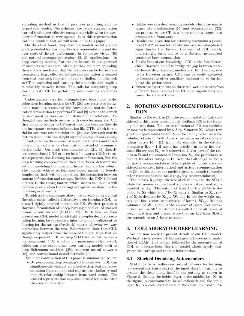
3.1 Stacked Denoising AutoencodersSDAE [32] is a feedforward neural network for learning

representations (encoding) of the input data by learning topredict the clean input itself in the output, as shown inFigure 2. Usually the hidden layer in the middle, i.e., X2 inthe figure, is constrained to be a bottleneck and the inputlayer X0 is a corrupted version of the clean input data. An

J

I

xL=2xL=2 xcxcx0x0

x0x0

x1x1

x2x2 xcxc

¸w¸w W+W+

¸v¸v

¸n¸n

vv RR

uu¸u¸u

J

I

xL=2xL=2x0x0

x0x0

x1x1

W+W+¸w¸w

vv¸v¸v RR

¸u¸u uu

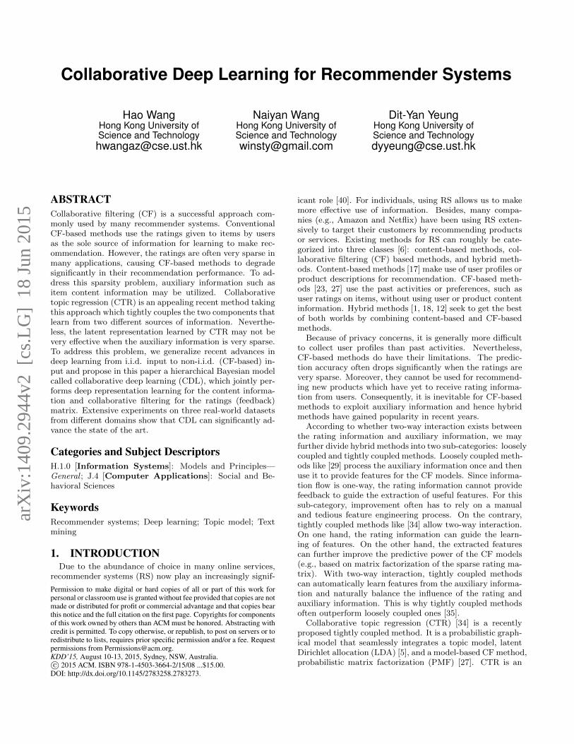
Figure 1: On the left is the graphical model of CDL. The part inside the dashed rectangle represents anSDAE. An example SDAE with L = 2 is shown. On the right is the graphical model of the degenerated CDL.The part inside the dashed rectangle represents the encoder of an SDAE. An example SDAE with L = 2 isshown on the right of it. Note that although L is still 2, the decoder of the SDAE vanishes. To preventclutter, we omit all variables xl except x0 and xL/2 in the graphical models.

X0X0 X1X1 X2X2 X3X3 X4X4 XcXc

Figure 2: A 2-layer SDAE with L = 4.

SDAE solves the following optimization problem:

min{Wl},{bl}

‖Xc −XL‖2F + λ∑l

‖Wl‖2F ,

where λ is a regularization parameter and ‖ · ‖F denotes theFrobenius norm.

3.2 Generalized Bayesian SDAEIf we assume that both the clean input Xc and the cor-

rupted input X0 are observed, similar to [4, 19, 3, 7], we candefine the following generative process:

1. For each layer l of the SDAE network,

(a) For each column n of the weight matrix Wl, draw

Wl,∗n ∼ N (0, λ−1w IKl).

(b) Draw the bias vector bl ∼ N (0, λ−1w IKl).

(c) For each row j of Xl, draw

Xl,j∗ ∼ N (σ(Xl−1,j∗Wl + bl), λ−1s IKl). (1)

2. For each item j, draw a clean input 1

Xc,j∗ ∼ N (XL,j∗, λ−1n IJ).

Note that if λs goes to infinity, the Gaussian distributionin Equation (1) will become a Dirac delta distribution [31]centered at σ(Xl−1,j∗Wl + bl), where σ(·) is the sigmoidfunction. The model will degenerate to be a Bayesian for-mulation of SDAE. That is why we call it generalized SDAE.

Note that the first L/2 layers of the network act as an en-coder and the last L/2 layers act as a decoder. Maximization

1Note that while generation of the clean input Xc from XL

is part of the generative process of the Bayesian SDAE, gen-eration of the noise-corrupted input X0 from Xc is an arti-ficial noise injection process to help the SDAE learn a morerobust feature representation.

of the posterior probability is equivalent to minimization ofthe reconstruction error with weight decay taken into con-sideration.

3.3 Collaborative Deep LearningUsing the Bayesian SDAE as a component, the generative

process of CDL is defined as follows:

1. For each layer l of the SDAE network,

(a) For each column n of the weight matrix Wl, draw

Wl,∗n ∼ N (0, λ−1w IKl).

(b) Draw the bias vector bl ∼ N (0, λ−1w IKl).

(c) For each row j of Xl, draw

Xl,j∗ ∼ N (σ(Xl−1,j∗Wl + bl), λ−1s IKl).

2. For each item j,

(a) Draw a clean input Xc,j∗ ∼ N (XL,j∗, λ−1n IJ).

(b) Draw a latent item offset vector εj ∼ N (0, λ−1v IK)

and then set the latent item vector to be:

vj = εj + XTL2,j∗.

3. Draw a latent user vector for each user i:

ui ∼ N (0, λ−1u IK).

4. Draw a rating Rij for each user-item pair (i, j):

Rij ∼ N (uTi vj ,C

−1ij ).

Here λw, λn, λu, λs, and λv are hyperparameters and Cij isa confidence parameter similar to that for CTR (Cij = a ifRij = 1 and Cij = b otherwise). Note that the middle layerXL/2 serves as a bridge between the ratings and content in-formation. This middle layer, along with the latent offset εj ,is the key that enables CDL to simultaneously learn an ef-fective feature representation and capture the similarity and(implicit) relationship between items (and users). Similar tothe generalized SDAE, for computational efficiency, we canalso take λs to infinity.

The graphical model of CDL when λs approaches positiveinfinity is shown in Figure 1, where, for notational simplicity,we use x0, xL/2, and xL in place of XT

0,j∗, XTL2,j∗, and XT

L,j∗,

respectively.

itemuser1

1

2

2

3

3

4

4

5

5

X 0X 0 X 1X 1 X 2X 2 X 3X 3 X 4X 4 X cX c

X 0X 0 X 1X 1 X 2X 2

corrupted

clean

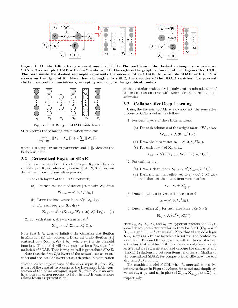
Figure 3: NN representation for degenerated CDL.

3.4 Maximum A Posteriori EstimatesBased on the CDL model above, all parameters could be

treated as random variables so that fully Bayesian methodssuch as Markov chain Monte Carlo (MCMC) or variationalapproximation methods [14] may be applied. However, suchtreatment typically incurs high computational cost. Besides,since CTR is our primary baseline for comparison, it wouldbe fair and reasonable to take an approach analogous to thatused in CTR. Consequently, we devise below an EM-stylealgorithm for obtaining the MAP estimates, as in [34].

Like in CTR, maximizing the posterior probability is equiv-alent to maximizing the joint log-likelihood of U, V, {Xl},Xc, {Wl}, {bl}, and R given λu, λv, λw, λs, and λn:

L =− λu

2

∑i

‖ui‖22 −λw

2

∑l

(‖Wl‖2F + ‖bl‖22)

− λv

2

∑j

‖vj −XTL2,j∗‖

22 −

λn

2

∑j

‖XL,j∗ −Xc,j∗‖22

− λs

2

∑l

∑j

‖σ(Xl−1,j∗Wl + bl)−Xl,j∗‖22

−∑i,j

Cij

2(Rij − uT

i vj)2.

If λs goes to infinity, the likelihood becomes:

L =− λu

2

∑i

‖ui‖22 −λw

2

∑l

(‖Wl‖2F + ‖bl‖22)

− λv

2

∑j

‖vj − fe(X0,j∗,W+)T ‖22

− λn

2

∑j

‖fr(X0,j∗,W+)−Xc,j∗‖22

−∑i,j

Cij

2(Rij − uT

i vj)2, (2)

where the encoder function fe(·,W+) takes the corruptedcontent vector X0,j∗ of item j as input and computes theencoding of the item, and the function fr(·,W+) also takesX0,j∗ as input, computes the encoding and then the recon-structed content vector of item j. For example, if the num-ber of layers L = 6, fe(X0,j∗,W

+) is the output of the thirdlayer while fr(X0,j∗,W

+) is the output of the sixth layer.From the perspective of optimization, the third term in

the objective function (2) above is equivalent to a multi-layerperceptron using the latent item vectors vj as target while

the fourth term is equivalent to an SDAE minimizing the re-construction error. Seeing from the view of neural networks(NN), when λs approaches positive infinity, training of theprobabilistic graphical model of CDL in Figure 1(left) woulddegenerate to simultaneously training two neural networksoverlaid together with a common input layer (the corruptedinput) but different output layers, as shown in Figure 3.Note that the second network is much more complex thantypical neural networks due to the involvement of the ratingmatrix.

When the ratio λn/λv approaches positive infinity, it willdegenerate to a two-step model in which the latent repre-sentation learned using SDAE is put directly into the CTR.Another extreme happens when λn/λv goes to zero wherethe decoder of the SDAE essentially vanishes. On the rightof Figure 1 is the graphical model of the degenerated CDLwhen λn/λv goes to zero. As demonstrated in the experi-ments, the predictive performance will suffer greatly for bothextreme cases.

For ui and vj , coordinate ascent similar to [34, 13] is used.Given the current W+, we compute the gradients of L withrespect to ui and vj and set them to zero, leading to thefollowing update rules:

ui ← (VCiVT + λuIK)−1VCiRi

vj ← (UCiUT + λvIK)−1(UCjRj + λvfe(X0,j∗,W

+)T ),

where U = (ui)Ii=1, V = (vj)

Jj=1, Ci = diag(Ci1, . . . ,CiJ)

is a diagonal matrix, Ri = (Ri1, . . . ,RiJ)T is a column vec-tor containing all the ratings of user i, and Cij reflects theconfidence controlled by a and b as discussed in [13].

Given U and V, we can learn the weights Wl and biasesbl for each layer using the back-propagation learning algo-rithm. The gradients of the likelihood with respect to Wl

and bl are as follows:

∇WlL = −λwWl

− λv

∑j

∇Wlfe(X0,j∗,W+)T (fe(X0,j∗,W

+)T − vj)

− λn

∑j

∇Wlfr(X0,j∗,W+)(fr(X0,j∗,W

+)−Xc,j∗)

∇blL = −λwbl

− λv

∑j

∇blfe(X0,j∗,W+)T (fe(X0,j∗,W

+)T − vj)

− λn

∑j

∇blfr(X0,j∗,W+)(fr(X0,j∗,W

+)−Xc,j∗).

By alternating the update of U, V, Wl, and bl, we can finda local optimum for L . Several commonly used techniquessuch as using a momentum term may be used to alleviate thelocal optimum problem. For completeness, we also providea sampling- based algorithm for CDL in the appendix.

3.5 PredictionLetD be the observed test data. Similar to [34], we use the

point estimates of ui, W+ and εj to calculate the predictedrating:

E[Rij |D] ≈ E[ui|D]T (E[fe(X0,j∗,W+)T |D] + E[εj |D]),

where E[·] denotes the expectation operation. In other words,

we approximate the predicted rating as:

R∗ij ≈ (u∗j )T (fe(X0,j∗,W+∗)T + ε∗j ) = (u∗i )Tv∗j .

Note that for any new item j with no rating in the trainingdata, its offset ε∗j will be 0.

4. EXPERIMENTSExtensive experiments are conducted on three real-world

datasets from different domains to demonstrate the effective-ness of our model both quantitatively and qualitatively2.

4.1 DatasetsWe use three datasets from different real-world domains,

two from CiteULike3 and one from Netflix, for our experi-ments. The first two datasets, from [35], were collected indifferent ways, specifically, with different scales and differentdegrees of sparsity to mimic different practical situations.The first dataset, citeulike-a, is mostly from [34]. The sec-ond dataset, citeulike-t, was collected independently of thefirst one. They manually selected 273 seed tags and collectedall the articles with at least one of those tags. Similar to [34],users with fewer than 3 articles are not included. As a re-sult, citeulike-a contains 5551 users and 16980 items. Forciteulike-t , the numbers are 7947 and 25975. We can see thatciteulike-t contains more users and items than citeulike-a.Also, citeulike-t is much sparser as only 0.07% of its user-item matrix entries contain ratings but citeulike-a has rat-ings in 0.22% of its user-item matrix entries.

The last dataset, Netflix, consists of two parts. The firstpart, with ratings and movie titles, is from the Netflix chal-lenge dataset. The second part, with plots of the corre-sponding movies, was collected by us from IMDB 4. Similarto [41], in order to be consistent with the implicit feedbacksetting of the first two datasets, we extract only positive rat-ings (rating 5) for training and testing. After removing userswith less than 3 positive ratings and movies without plots,we have 407261 users, 9228 movies, and 15348808 ratings inthe final dataset.

We follow the same procedure as that in [34] to preprocessthe text information (item content) extracted from the ti-tles and abstracts of the articles and the plots of the movies.After removing stop words, the top S discriminative wordsaccording to the tf-idf values are chosen to form the vocab-ulary (S is 8000, 20000, and 20000 for the three datasets).

4.2 Evaluation SchemeFor each dataset, similar to [35, 36], we randomly select

P items associated with each user to form the training setand use all the rest of the dataset as the test set. To eval-uate and compare the models under both sparse and densesettings, we set P to 1 and 10, respectively, in our experi-ments. For each value of P , we repeat the evaluation fivetimes with different randomly selected training sets and theaverage performance is reported.

As in [34, 22, 35], we use recall as the performance measurebecause the rating information is in the form of implicit

2Code and data are available at www.wanghao.in3CiteULike allows users to create their own collections ofarticles. There are abstract, title, and tags for each arti-cle. More details about the CiteULike data can be found athttp://www.citeulike.org.4http://www.imdb.com

feedback [13, 23]. Specifically, a zero entry may be due tothe fact that the user is not interested in the item, or that theuser is not aware of its existence. As such, precision is nota suitable performance measure. Like most recommendersystems, we sort the predicted ratings of the candidate itemsand recommend the top M items to the target user. Therecall@M for each user is then defined as:

recall@M =number of items that the user likes among the top M

total number of items that the user likes.

The final result reported is the average recall over all users.Another evaluation metric is the mean average precision

(mAP). Exactly the same as [21], we set the cutoff point at500 for each user.

4.3 Baselines and Experimental SettingsThe models included in our comparison are listed as fol-

lows:• CMF: Collective Matrix Factorization [30] is a model

incorporating different sources of information by simul-taneously factorizing multiple matrices. In this paper,the two factorized matrices are R and Xc.• SVDFeature: SVDFeature [8] is a model for feature-

based collaborative filtering. In this paper we use thecontent information Xc as raw features to feed intoSVDFeature.• DeepMusic: DeepMusic [21] is a model for music rec-

ommendation mentioned in Section 1. We use the vari-ant, a loosely coupled method, that achieves the bestperformance as our baseline.• CTR: Collaborative Topic Regression [34] is a model

performing topic modeling and collaborative filteringsimultaneously as mentioned in the previous section.• CDL: Collaborative Deep Learning is our proposed

model as described above. It allows different levels ofmodel complexity by varying the number of layers.

In the experiments, we first use a validation set to findthe optimal hyperparameters for CMF, SVDFeature, CTR,and DeepMusic. For CMF, we set the regularization hyper-parameters for the latent factors of different contexts to 10.After the grid search, we find that CMF performs best whenthe weights for the rating matrix and content matrix (BOW)are both 5 in the sparse setting. For the dense setting theweights are 8 and 2, respectively. For SVDFeature, the bestperformance is achieved when the regularization hyperpa-rameters for the users and items are both 0.004 with thelearning rate equal to 0.005. For DeepMusic, we find thatthe best performance is achieved using a CNN with two con-volutional layers. We also try our best to tune the other hy-perparameters. For CTR, we find that it can achieve goodprediction performance when λu = 0.1, λv = 10, a = 1,b = 0.01, and K = 50 (note that a and b determine the con-fidence parameters Cij). For CDL, we directly set a = 1,b = 0.01, K = 50 and perform grid search on the hyperpa-rameters λu, λv, λn, and λw. For the grid search, we splitthe training data and use 5-fold cross validation.

We use a masking noise with a noise level of 0.3 to get thecorrupted input X0 from the clean input Xc. For CDL withmore than one layer of SDAE (L > 2), we use a dropout rate[2, 33, 11] of 0.1 to achieve adaptive regularization. In termsof network architecture, the number of hidden units Kl is setto 200 for l such that l 6= L/2 and 0 < l < L. While both K0

and KL are equal to the number of words S in the dictionary,KL/2 is set to K which is the number of dimensions of the

50 100 150 200 250 300

0.05

0.1

0.15

0.2

0.25

0.3

M

Rec

all

CDLCTRDeepMusicCMFSVDFeature

50 100 150 200 250 300

0.05

0.1

0.15

0.2

0.25

0.3

M

Rec

all

CDLCTRDeepMusicCMFSVDFeature

50 100 150 200 250 3000

0.05

0.1

0.15

0.2

0.25

0.3

M

Rec

all

CDLCTRDeepMusicCMFSVDFeature

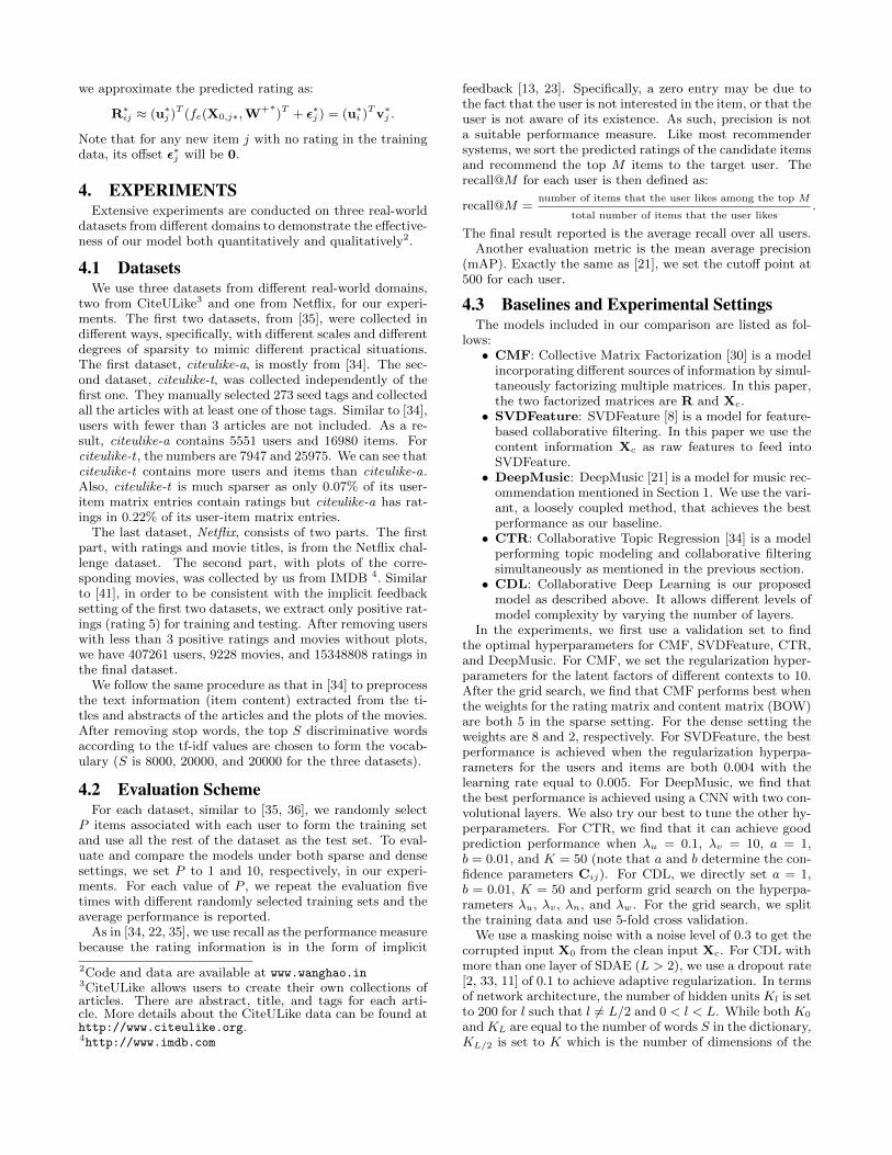
Figure 4: Performance comparison of CDL, CTR, DeepMusic, CMF, and SVDFeature based on recall@Mfor datasets citeulike-a, citeulike-t, and Netflix in the sparse setting. A 2-layer CDL is used.

50 100 150 200 250 300

0.15

0.2

0.25

0.3

0.35

0.4

0.45

0.5

0.55

M

Rec

all

CDLCTRDeepMusicCMFSVDFeature

50 100 150 200 250 300

0.05

0.1

0.15

0.2

0.25

0.3

0.35

0.4

0.45

0.5

M

Rec

all

CDLCTRDeepMusicCMFSVDFeature

50 100 150 200 250 300

0.2

0.25

0.3

0.35

0.4

0.45

0.5

0.55

0.6

0.65

0.7

M

Rec

all

CDLCTRDeepMusicCMFSVDFeature

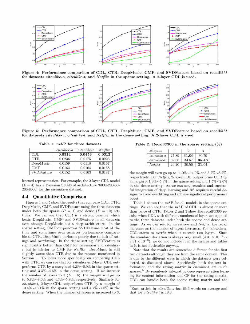
Figure 5: Performance comparison of CDL, CTR, DeepMusic, CMF, and SVDFeature based on recall@Mfor datasets citeulike-a, citeulike-t, and Netflix in the dense setting. A 2-layer CDL is used.

Table 1: mAP for three datasets

citeulike-a citeulike-t NetflixCDL 0.0514 0.0453 0.0312CTR 0.0236 0.0175 0.0223DeepMusic 0.0159 0.0118 0.0167CMF 0.0164 0.0104 0.0158SVDFeature 0.0152 0.0103 0.0187

learned representation. For example, the 2-layer CDL model(L = 4) has a Bayesian SDAE of architecture ‘8000-200-50-200-8000’ for the citeulike-a dataset.

4.4 Quantitative ComparisonFigures 4 and 5 show the results that compare CDL, CTR,

DeepMusic, CMF, and SVDFeature using the three datasetsunder both the sparse (P = 1) and dense (P = 10) set-tings. We can see that CTR is a strong baseline whichbeats DeepMusic, CMF, and SVDFeature in all datasetseven though DeepMusic has a deep architecture. In thesparse setting, CMF outperforms SVDFeature most of thetime and sometimes even achieves performance compara-ble to CTR. DeepMusic performs poorly due to lack of rat-ings and overfitting. In the dense setting, SVDFeature issignificantly better than CMF for citeulike-a and citeulike-t but is inferior to CMF for Netflix. DeepMusic is stillslightly worse than CTR due to the reasons mentioned inSection 1. To focus more specifically on comparing CDLwith CTR, we can see that for citeulike-a, 2-layer CDL out-performs CTR by a margin of 4.2%∼6.0% in the sparse set-ting and 3.3%∼4.6% in the dense setting. If we increasethe number of layers to 3 (L = 6), the margin will go upto 5.8%∼8.0% and 4.3%∼5.8%, respectively. Similarly forciteulike-t, 2-layer CDL outperforms CTR by a margin of10.4%∼13.1% in the sparse setting and 4.7%∼7.6% in thedense setting. When the number of layers is increased to 3,

Table 2: Recall@300 in the sparse setting (%)

#layers 1 2 3citeulike-a 27.89 31.06 30.70citeulike-t 32.58 34.67 35.48Netflix 29.20 30.50 31.01

the margin will even go up to 11.0%∼14.9% and 5.2%∼8.2%,respectively. For Netflix, 2-layer CDL outperforms CTR bya margin of 1.9%∼5.9% in the sparse setting and 1.5%∼2.0%in the dense setting. As we can see, seamless and success-ful integration of deep learning and RS requires careful de-signs to avoid overfitting and achieve significant performanceboost.

Table 1 shows the mAP for all models in the sparse set-tings. We can see that the mAP of CDL is almost or morethan twice of CTR. Tables 2 and 3 show the recall@300 re-sults when CDL with different numbers of layers are appliedto the three datasets under both the sparse and dense set-tings. As we can see, for citeulike-t and Netflix, the recallincreases as the number of layers increases. For citeulike-a,CDL starts to overfit when it exceeds two layers. Sincethe standard deviation is always very small (4.31 × 10−5 ∼9.31 × 10−3), we do not include it in the figures and tablesas it is not noticeable anyway.

Note that the results are somewhat different for the firsttwo datasets although they are from the same domain. Thisis due to the different ways in which the datasets were col-lected, as discussed above. Specifically, both the text in-formation and the rating matrix in citeulike-t are muchsparser.5 By seamlessly integrating deep representation learn-ing for content information and CF for the rating matrix,CDL can handle both the sparse rating matrix and the

5Each article in citeulike-a has 66.6 words on average andthat for citeulike-t is 18.8.

50 100 150 200 250 300

0.2

0.25

0.3

0.35

0.4

0.45

0.5

M

Rec

all

λn = 104

λn = 102

λn = 100

λn = 10−2

PMF

50 100 150 200 250 300

0.25

0.3

0.35

0.4

0.45

0.5

M

Rec

all

λn = 104

λn = 103

λn = 102

λn = 101

PMF

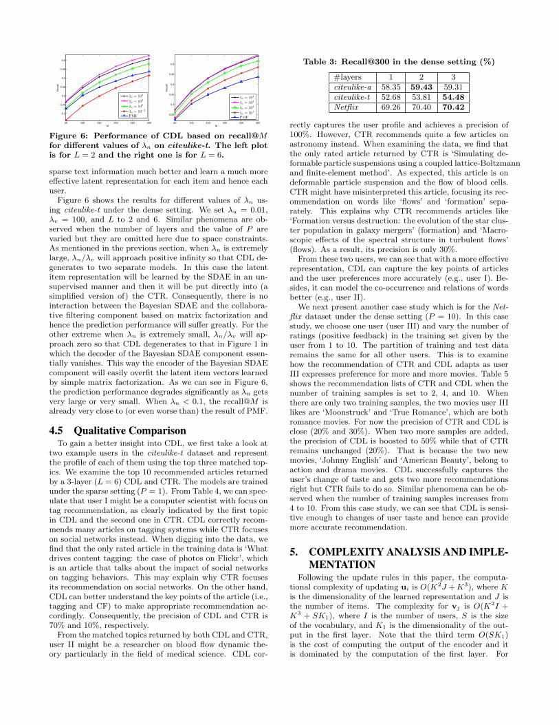
Figure 6: Performance of CDL based on recall@Mfor different values of λn on citeulike-t. The left plotis for L = 2 and the right one is for L = 6.

sparse text information much better and learn a much moreeffective latent representation for each item and hence eachuser.

Figure 6 shows the results for different values of λn us-ing citeulike-t under the dense setting. We set λu = 0.01,λv = 100, and L to 2 and 6. Similar phenomena are ob-served when the number of layers and the value of P arevaried but they are omitted here due to space constraints.As mentioned in the previous section, when λn is extremelylarge, λn/λv will approach positive infinity so that CDL de-generates to two separate models. In this case the latentitem representation will be learned by the SDAE in an un-supervised manner and then it will be put directly into (asimplified version of) the CTR. Consequently, there is nointeraction between the Bayesian SDAE and the collabora-tive filtering component based on matrix factorization andhence the prediction performance will suffer greatly. For theother extreme when λn is extremely small, λn/λv will ap-proach zero so that CDL degenerates to that in Figure 1 inwhich the decoder of the Bayesian SDAE component essen-tially vanishes. This way the encoder of the Bayesian SDAEcomponent will easily overfit the latent item vectors learnedby simple matrix factorization. As we can see in Figure 6,the prediction performance degrades significantly as λn getsvery large or very small. When λn < 0.1, the recall@M isalready very close to (or even worse than) the result of PMF.

4.5 Qualitative ComparisonTo gain a better insight into CDL, we first take a look at

two example users in the citeulike-t dataset and representthe profile of each of them using the top three matched top-ics. We examine the top 10 recommended articles returnedby a 3-layer (L = 6) CDL and CTR. The models are trainedunder the sparse setting (P = 1). From Table 4, we can spec-ulate that user I might be a computer scientist with focus ontag recommendation, as clearly indicated by the first topicin CDL and the second one in CTR. CDL correctly recom-mends many articles on tagging systems while CTR focuseson social networks instead. When digging into the data, wefind that the only rated article in the training data is ‘Whatdrives content tagging: the case of photos on Flickr’, whichis an article that talks about the impact of social networkson tagging behaviors. This may explain why CTR focusesits recommendation on social networks. On the other hand,CDL can better understand the key points of the article (i.e.,tagging and CF) to make appropriate recommendation ac-cordingly. Consequently, the precision of CDL and CTR is70% and 10%, respectively.

From the matched topics returned by both CDL and CTR,user II might be a researcher on blood flow dynamic the-ory particularly in the field of medical science. CDL cor-

Table 3: Recall@300 in the dense setting (%)

#layers 1 2 3citeulike-a 58.35 59.43 59.31citeulike-t 52.68 53.81 54.48Netflix 69.26 70.40 70.42

rectly captures the user profile and achieves a precision of100%. However, CTR recommends quite a few articles onastronomy instead. When examining the data, we find thatthe only rated article returned by CTR is ‘Simulating de-formable particle suspensions using a coupled lattice-Boltzmannand finite-element method’. As expected, this article is ondeformable particle suspension and the flow of blood cells.CTR might have misinterpreted this article, focusing its rec-ommendation on words like ‘flows’ and ‘formation’ sepa-rately. This explains why CTR recommends articles like‘Formation versus destruction: the evolution of the star clus-ter population in galaxy mergers’ (formation) and ‘Macro-scopic effects of the spectral structure in turbulent flows’(flows). As a result, its precision is only 30%.

From these two users, we can see that with a more effectiverepresentation, CDL can capture the key points of articlesand the user preferences more accurately (e.g., user I). Be-sides, it can model the co-occurrence and relations of wordsbetter (e.g., user II).

We next present another case study which is for the Net-flix dataset under the dense setting (P = 10). In this casestudy, we choose one user (user III) and vary the number ofratings (positive feedback) in the training set given by theuser from 1 to 10. The partition of training and test dataremains the same for all other users. This is to examinehow the recommendation of CTR and CDL adapts as userIII expresses preference for more and more movies. Table 5shows the recommendation lists of CTR and CDL when thenumber of training samples is set to 2, 4, and 10. Whenthere are only two training samples, the two movies user IIIlikes are ‘Moonstruck’ and ‘True Romance’, which are bothromance movies. For now the precision of CTR and CDL isclose (20% and 30%). When two more samples are added,the precision of CDL is boosted to 50% while that of CTRremains unchanged (20%). That is because the two newmovies, ‘Johnny English’ and ‘American Beauty’, belong toaction and drama movies. CDL successfully captures theuser’s change of taste and gets two more recommendationsright but CTR fails to do so. Similar phenomena can be ob-served when the number of training samples increases from4 to 10. From this case study, we can see that CDL is sensi-tive enough to changes of user taste and hence can providemore accurate recommendation.

5. COMPLEXITY ANALYSIS AND IMPLE-MENTATION

Following the update rules in this paper, the computa-tional complexity of updating ui is O(K2J +K3), where Kis the dimensionality of the learned representation and J isthe number of items. The complexity for vj is O(K2I +K3 + SK1), where I is the number of users, S is the sizeof the vocabulary, and K1 is the dimensionality of the out-put in the first layer. Note that the third term O(SK1)is the cost of computing the output of the encoder and itis dominated by the computation of the first layer. For

Table 4: Interpretability of the latent structures learned

user I (CDL) in user’s lib?

top 3 topics1. search, image, query, images, queries, tagging, index, tags, searching, tag2. social, online, internet, communities, sharing, networking, facebook, friends, ties, participation3. collaborative, optimization, filtering, recommendation, contextual, planning, items, preferences

top 10 articles

1. The structure of collaborative tagging Systems yes2. Usage patterns of collaborative tagging systems yes3. Folksonomy as a complex network no4. HT06, tagging paper, taxonomy, Flickr, academic article, to read yes5. Why do tagging systems work yes6. Information retrieval in folksonomies: search and ranking no7. tagging, communities, vocabulary, evolution yes8. The complex dynamics of collaborative tagging yes9. Improved annotation of the blogosphere via autotagging and hierarchical clustering no10. Collaborative tagging as a tripartite network yes

user I (CTR) in user’s lib?

top 3 topics1. social, online, internet, communities, sharing, networking, facebook, friends, ties, participation2. search, image, query, images, queries, tagging, index, tags, searching, tag3. feedback, event, transformation, wikipedia, indicators, vitamin, log, indirect, taxonomy

top 10 articles

1. HT06, tagging paper, taxonomy, Flickr, academic article, to read yes2. Structure and evolution of online social networks no3. Group formation in large social networks: membership, growth, and evolution no4. Measurement and analysis of online social networks no5. A face(book) in the crowd: social searching vs. social browsing no6. The strength of weak ties no7. Flickr tag recommendation based on collective knowledge no8. The computer-mediated communication network no9. Social capital, self-esteem, and use of online social network sites: A longitudinal analysis no10. Increasing participation in online communities: A framework for human-computer interaction no

user II (CDL) in user’s lib?

top 3 topics1. flow, cloud, codes, matter, boundary, lattice, particles, galaxies, fluid, galaxy2. mobile, membrane, wireless, sensor, mobility, lipid, traffic, infrastructure, monitoring, ad3. hybrid, orientation, stress, fluctuations, load, temperature, centrality, mechanical, two-dimensional, heat

top 10 articles

1. Modeling the flow of dense suspensions of deformable particles in three dimensions yes2. Simplified particulate model for coarse-grained hemodynamics simulations yes3. Lattice Boltzmann simulations of blood flow: non-newtonian rheology and clotting processes yes4. A genome-wide association study for celiac disease identifies risk variants yes5. Efficient and accurate simulations of deformable particles yes6. A multiscale model of thrombus development yes7. Multiphase hemodynamic simulation of pulsatile flow in a coronary artery yes8. Lattice Boltzmann modeling of thrombosis in giant aneurysms yes9. A lattice Boltzmann simulation of clotting in stented aneursysms yes10. Predicting dynamics and rheology of blood flow yes

user II (CTR) in user’s lib?

top 3 topics1. flow, cloud, codes, matter, boundary, lattice, particles, galaxies, fluid, galaxy2. transition, equations, dynamical, discrete, equation, dimensions, chaos, transitions, living, trust3. mobile, membrane, wireless, sensor, mobility, lipid, traffic, infrastructure, monitoring, ad

top 10 articles

1. Multiphase hemodynamic simulation of pulsatile flow in a coronary artery yes2. The metallicity evolution of star-forming galaxies from redshift 0 to 3 no3. Formation versus destruction: the evolution of the star cluster population in galaxy mergers no4. Clearing the gas from globular clusters no5. Macroscopic effects of the spectral structure in turbulent flows no6. The WiggleZ dark energy survey no7. Lattice-Boltzmann simulation of blood flow in digitized vessel networks no8. Global properties of ’ordinary’ early-type galaxies no9. Proteus : a direct forcing method in the simulations of particulate flows yes10. Analysis of mechanisms for platelet near-wall excess under arterial blood flow conditions yes

the update of all the weights and biases, the complexityis O(JSK1) since the computation is dominated by the firstlayer. Thus for a complete epoch the total time complexityis O(JSK1 +K2J2 +K2I2 +K3).

All our experiments are conducted on servers with 2 In-tel E5-2650 CPUs and 4 NVIDIA Tesla M2090 GPUs each.Using the MATLAB implementation with GPU/C++ ac-celeration, each epoch takes only about 40 seconds and eachrun takes 200 epochs for the first two datasets. For Netflixit takes about 60 seconds per epoch and needs much fewerepochs (about 100) to get satisfactory recommendation per-formance. Since Netflix is much larger than the other twodatasets, this shows that CDL is very scalable. We expectthat changing the implementation to a pure C++/CUDAone would significantly reduce the time cost.

6. CONCLUSION AND FUTURE WORKWe have demonstrated in this paper that state-of-the-art

performance can be achieved by jointly performing deep rep-resentation learning for the content information and collab-orative filtering for the ratings (feedback) matrix. As faras we know, CDL is the first hierarchical Bayesian model tobridge the gap between state-of-the-art deep learning modelsand RS. In terms of learning, besides the algorithm for at-taining the MAP estimates, we also derive a sampling-basedalgorithm for the Bayesian treatment of CDL as a Bayesiangeneralized version of back-propagation.

Among the possible extensions that could be made toCDL, the bag-of-words representation may be replaced bymore powerful alternatives, such as [20]. The Bayesian na-ture of CDL also provides potential performance boost ifother side information is incorporated as in [37]. Besides, as

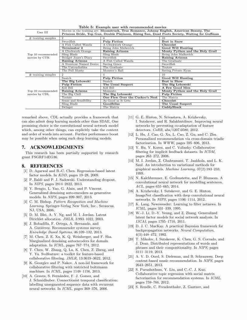
Table 5: Example user with recommended movies

User IIIMovies in the training set: Moonstruck, True Romance, Johnny English, American Beauty, ThePrincess Bride, Top Gun, Double Platinum, Rising Sun, Dead Poets Society, Waiting for Guffman

# training samples 2 4 10

Top 10 recommendedmovies by CTR

Swordfish Pulp Fiction Best in SnowA Fish Called Wanda A Clockwork Orange ChocolatTerminator 2 Being John Malkovich Good Will HuntingA Clockwork Orange Raising Arizona Monty Python and the Holy GrailSling Blade Sling Blade Being John MalkovichBridget Jones’s Diary Swordfish Raising ArizonaRaising Arizona A Fish Called Wanda The GraduateA Streetcar Named Desire Saving Grace SwordfishThe Untouchables The Graduate TootsieThe Full Monty Monster’s Ball Saving Private Ryan

# training samples 2 4 10

Top 10 recommendedmovies by CDL

Snatch Pulp Fiction Good Will HuntingThe Big Lebowski Snatch Best in ShowPulp Fiction The Usual Suspect The Big LebowskiKill Bill Kill Bill A Few Good MenRaising Arizona Momento Monty Python and the Holy GrailThe Big Chill The Big Lebowski Pulp FictionTootsie One Flew Over the Cuckoo’s Nest The MatrixSense and Sensibility As Good as It Gets ChocolatSling Blade Goodfellas The Usual SuspectSwinger The Matrix CaddyShack

remarked above, CDL actually provides a framework thatcan also admit deep learning models other than SDAE. Onepromising choice is the convolutional neural network modelwhich, among other things, can explicitly take the contextand order of words into account. Further performance boostmay be possible when using such deep learning models.

7. ACKNOWLEDGMENTSThis research has been partially supported by research

grant FSGRF14EG36.

8. REFERENCES[1] D. Agarwal and B.-C. Chen. Regression-based latent

factor models. In KDD, pages 19–28, 2009.

[2] P. Baldi and P. J. Sadowski. Understanding dropout.In NIPS, pages 2814–2822, 2013.

[3] Y. Bengio, L. Yao, G. Alain, and P. Vincent.Generalized denoising auto-encoders as generativemodels. In NIPS, pages 899–907, 2013.

[4] C. M. Bishop. Pattern Recognition and MachineLearning. Springer-Verlag New York, Inc., Secaucus,NJ, USA, 2006.

[5] D. M. Blei, A. Y. Ng, and M. I. Jordan. LatentDirichlet allocation. JMLR, 3:993–1022, 2003.

[6] J. Bobadilla, F. Ortega, A. Hernando, andA. Gutierrez. Recommender systems survey.Knowledge Based Systems, 46:109–132, 2013.

[7] M. Chen, Z. E. Xu, K. Q. Weinberger, and F. Sha.Marginalized denoising autoencoders for domainadaptation. In ICML, pages 767–774, 2012.

[8] T. Chen, W. Zhang, Q. Lu, K. Chen, Z. Zheng, andY. Yu. Svdfeature: a toolkit for feature-basedcollaborative filtering. JMLR, 13:3619–3622, 2012.

[9] K. Georgiev and P. Nakov. A non-iid framework forcollaborative filtering with restricted boltzmannmachines. In ICML, pages 1148–1156, 2013.

[10] A. Graves, S. Fernandez, F. J. Gomez, andJ. Schmidhuber. Connectionist temporal classification:labelling unsegmented sequence data with recurrentneural networks. In ICML, pages 369–376, 2006.

[11] G. E. Hinton, N. Srivastava, A. Krizhevsky,I. Sutskever, and R. Salakhutdinov. Improving neuralnetworks by preventing co-adaptation of featuredetectors. CoRR, abs/1207.0580, 2012.

[12] L. Hu, J. Cao, G. Xu, L. Cao, Z. Gu, and C. Zhu.Personalized recommendation via cross-domain triadicfactorization. In WWW, pages 595–606, 2013.

[13] Y. Hu, Y. Koren, and C. Volinsky. Collaborativefiltering for implicit feedback datasets. In ICDM,pages 263–272, 2008.

[14] M. I. Jordan, Z. Ghahramani, T. Jaakkola, and L. K.Saul. An introduction to variational methods forgraphical models. Machine Learning, 37(2):183–233,1999.

[15] N. Kalchbrenner, E. Grefenstette, and P. Blunsom. Aconvolutional neural network for modelling sentences.ACL, pages 655–665, 2014.

[16] A. Krizhevsky, I. Sutskever, and G. E. Hinton.ImageNet classification with deep convolutional neuralnetworks. In NIPS, pages 1106–1114, 2012.

[17] K. Lang. Newsweeder: Learning to filter netnews. InICML, pages 331–339, 1995.

[18] W.-J. Li, D.-Y. Yeung, and Z. Zhang. Generalizedlatent factor models for social network analysis. InIJCAI, pages 1705–1710, 2011.

[19] D. J. C. MacKay. A practical Bayesian framework forbackpropagation networks. Neural Computation,4(3):448–472, 1992.

[20] T. Mikolov, I. Sutskever, K. Chen, G. S. Corrado, andJ. Dean. Distributed representations of words andphrases and their compositionality. In NIPS, pages3111–3119, 2013.

[21] A. V. D. Oord, S. Dieleman, and B. Schrauwen. Deepcontent-based music recommendation. In NIPS, pages2643–2651, 2013.

[22] S. Purushotham, Y. Liu, and C.-C. J. Kuo.Collaborative topic regression with social matrixfactorization for recommendation systems. In ICML,pages 759–766, 2012.

[23] S. Rendle, C. Freudenthaler, Z. Gantner, and

L. Schmidt-Thieme. BPR: Bayesian personalizedranking from implicit feedback. In UAI, pages452–461, 2009.

[24] T. N. Sainath, B. Kingsbury, V. Sindhwani, E. Arisoy,and B. Ramabhadran. Low-rank matrix factorizationfor deep neural network training withhigh-dimensional output targets. In ICASSP, pages6655–6659, 2013.

[25] R. Salakhutdinov and G. E. Hinton. Deep Boltzmannmachines. In AISTATS, pages 448–455, 2009.

[26] R. Salakhutdinov and G. E. Hinton. Semantic hashing.Int. J. Approx. Reasoning, 50(7):969–978, 2009.

[27] R. Salakhutdinov and A. Mnih. Probabilistic matrixfactorization. In NIPS, pages 1257–1264, 2007.

[28] R. Salakhutdinov, A. Mnih, and G. E. Hinton.Restricted boltzmann machines for collaborativefiltering. In ICML, pages 791–798, 2007.

[29] S. G. Sevil, O. Kucuktunc, P. Duygulu, and F. Can.Automatic tag expansion using visual similarity forphoto sharing websites. Multimedia Tools Appl.,49(1):81–99, 2010.

[30] A. P. Singh and G. J. Gordon. Relational learning viacollective matrix factorization. In KDD, pages650–658, 2008.

[31] R. S. Strichartz. A Guide to Distribution Theory andFourier Transforms. World Scientific, 2003.

[32] P. Vincent, H. Larochelle, I. Lajoie, Y. Bengio, andP.-A. Manzagol. Stacked denoising autoencoders:Learning useful representations in a deep network witha local denoising criterion. JMLR, 11:3371–3408, 2010.

[33] S. Wager, S. Wang, and P. Liang. Dropout training asadaptive regularization. In NIPS, pages 351–359, 2013.

[34] C. Wang and D. M. Blei. Collaborative topic modelingfor recommending scientific articles. In KDD, pages448–456, 2011.

[35] H. Wang, B. Chen, and W.-J. Li. Collaborative topicregression with social regularization for tagrecommendation. In IJCAI, pages 2719–2725, 2013.

[36] H. Wang and W. Li. Relational collaborative topicregression for recommender systems. TKDE,27(5):1343–1355, 2015.

[37] H. Wang, X. Shi, and D. Yeung. Relational stackeddenoising autoencoder for tag recommendation. InAAAI, pages 3052–3058, 2015.

[38] N. Wang and D.-Y. Yeung. Learning a deep compactimage representation for visual tracking. In NIPS,pages 809–817, 2013.

[39] X. Wang and Y. Wang. Improving content-based andhybrid music recommendation using deep learning. InACM MM, pages 627–636, 2014.

[40] W. Zhang, H. Sun, X. Liu, and X. Guo. Temporalqos-aware web service recommendation vianon-negative tensor factorization. In WWW, pages585–596, 2014.

[41] K. Zhou and H. Zha. Learning binary codes forcollaborative filtering. In KDD, pages 498–506, 2012.

APPENDIXA. BAYESIAN TREATMENT FOR CDL

For completeness we also derive a sampling-based algo-

−15 −10 −5 0 50

0.05

0.1

0.15

0.2

0.25

0.3

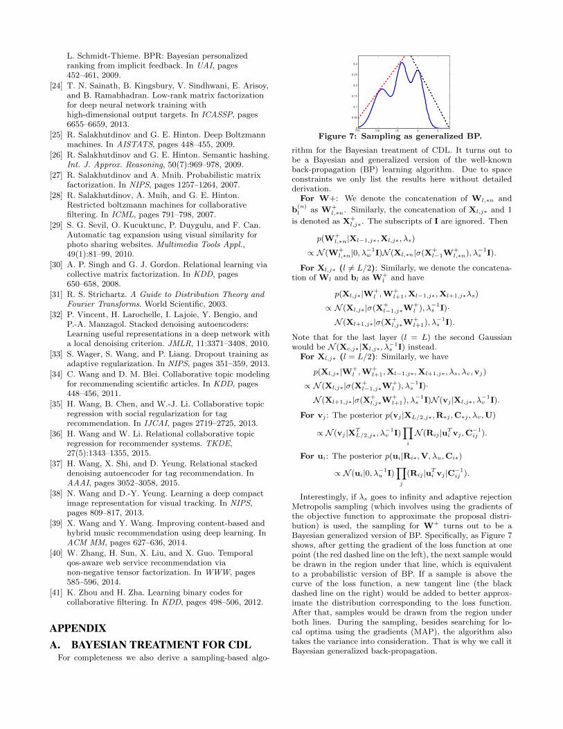
Figure 7: Sampling as generalized BP.

rithm for the Bayesian treatment of CDL. It turns out tobe a Bayesian and generalized version of the well-knownback-propagation (BP) learning algorithm. Due to spaceconstraints we only list the results here without detailedderivation.

For W+: We denote the concatenation of Wl,∗n and

b(n)l as W+

l,∗n. Similarly, the concatenation of Xl,j∗ and 1

is denoted as X+l,j∗. The subscripts of I are ignored. Then

p(W+l,∗n|Xl−1,j∗,Xl,j∗, λs)

∝ N (W+l,∗n|0, λ

−1w I)N (Xl,∗n|σ(X+

l−1W+l,∗n), λ−1

s I).

For Xl,j∗ (l 6= L/2): Similarly, we denote the concatena-tion of Wl and bl as W+

l and have

p(Xl,j∗|W+l ,W

+l+1,Xl−1,j∗,Xl+1,j∗λs)

∝ N (Xl,j∗|σ(X+l−1,j∗W

+l ), λ−1

s I)·

N (Xl+1,j∗|σ(X+l,j∗W

+l+1), λ−1

s I).

Note that for the last layer (l = L) the second Gaussianwould be N (Xc,j∗|Xl,j∗, λ

−1s I) instead.

For Xl,j∗ (l = L/2): Similarly, we have

p(Xl,j∗|W+l ,W

+l+1,Xl−1,j∗,Xl+1,j∗, λs, λv,vj)

∝ N (Xl,j∗|σ(X+l−1,j∗W

+l ), λ−1

s I)·

N (Xl+1,j∗|σ(X+l,j∗W

+l+1), λ−1

s I)N (vj |Xl,j∗, λ−1v I).

For vj : The posterior p(vj |XL/2,j∗,R∗j ,C∗j , λv,U)

∝ N (vj |XTL/2,j∗, λ

−1v I)

∏i

N (Rij |uTi vj ,C

−1ij ).

For ui: The posterior p(ui|Ri∗,V, λu,Ci∗)

∝ N (ui|0, λ−1u I)

∏j

(Rij |uTi vj |C−1

ij ).

Interestingly, if λs goes to infinity and adaptive rejectionMetropolis sampling (which involves using the gradients ofthe objective function to approximate the proposal distri-bution) is used, the sampling for W+ turns out to be aBayesian generalized version of BP. Specifically, as Figure 7shows, after getting the gradient of the loss function at onepoint (the red dashed line on the left), the next sample wouldbe drawn in the region under that line, which is equivalentto a probabilistic version of BP. If a sample is above thecurve of the loss function, a new tangent line (the blackdashed line on the right) would be added to better approx-imate the distribution corresponding to the loss function.After that, samples would be drawn from the region underboth lines. During the sampling, besides searching for lo-cal optima using the gradients (MAP), the algorithm alsotakes the variance into consideration. That is why we call itBayesian generalized back-propagation.