Coherent activity in excitatory neural networksâ€™

Coherent activity in excitatoryneural networks’

Alessandro Torcini

Istituto dei Sistemi Complessi - CNR - Firenze

Marie-Curie ITN-FP7 NETT Project

Nottingham 2013 – p. 1

Effects of excitatory coupling

When Inhibition and not Excitation Synchronizes Neural Firing

In this paper of 1994 by Van Vreeswijk, Abbott, and Ermentrout the authors affirm:

It is commonly believed that excitatory synaptic coupling tend to synchronizeneural firing, while inhibitory coupling pushes the neurons toward anti-synchrony

However, in the reticular nucleus of the thalamus, synchronized oscillations occurvia purely inhibitory coupling [Wang and Rinzel (1992)]

For two coupled neurons we will show that such reversed behaviour is the rulerather than the exception

Which is the situation for large populations of neurons ?


Collective Dynamics in the Brain

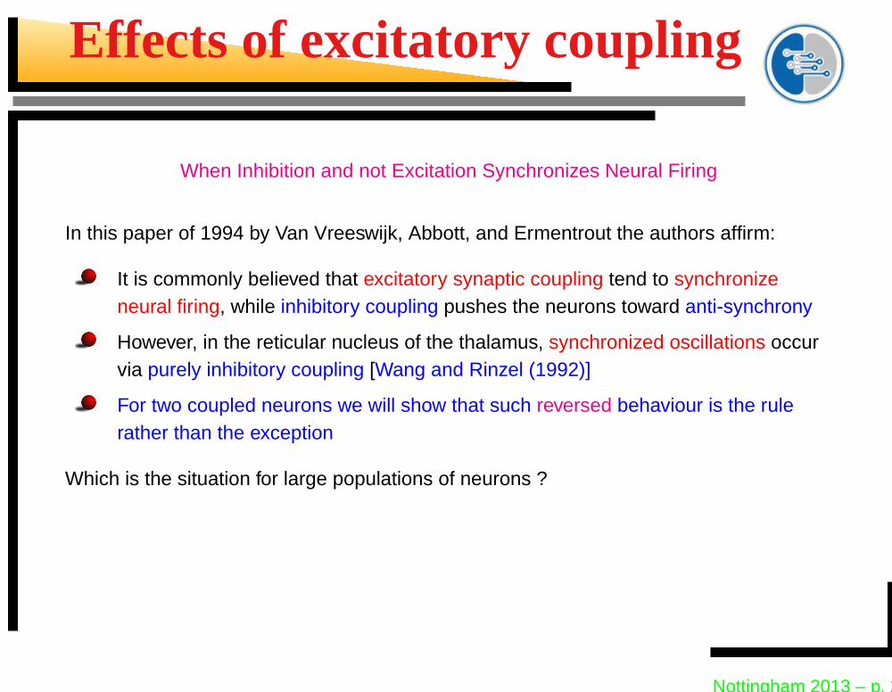
Rhythmic coherent dynamical behaviours have been widely identified in differentneuronal populations in the mammalian brain [G. Buszaki - Rhythms of the Brain]

Collective oscillations are commonly associated with the inhibitory role ofinterneurons

Pure excitatory interactions are believed to lead to abnormal synchronization of theneural population associated with epileptic seizures in the cerebral cortex

However, coherent activity patterns havebeen observed also in “in vivo” measure-ments of the developing rodent neocortexand hyppocampus for a short period afterbirth, despite the fact that at this early stagethe nature of the involved synapses is essen-tially excitatory [C. Allene et al., The Journalof Neuroscience (2008)]

Calcium fluorescence tracestwo-photon laser microscopy


Summary

We analyze pulse-coupled leaky integrate-and-fire (LIF) neurons

Analysis of the dynamics of two coupled neurons

LIF neuronal models coupled

α pulses and exponential pulses

inhibitory and excitatory coupling

Hodgkin-Huxley coupled neurons

Van Vreeswijk, Abbott, Ermentout, JCN (1994);

Hansel, Mato, Meunier, Neural computation (1995)

Emergence of collective solution in fully coupled networks of LIF neurons

Splay states

Coherent collective solutions - Partial Synchronization

Abbott - van Vreeswijk, Physical Review E (1993)

Mohanty, Politi EurophysLett (2006)

Zillmer et al. Physical Review E (2007)


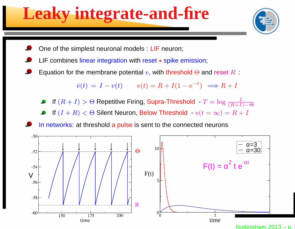
Leaky integrate-and-fire

One of the simplest neuronal models : LIF neuron;

LIF combines linear integration with reset + spike emission;

Equation for the membrane potential v, with threshold Θ and reset R :

v(t) = I − v(t) v(t) = R + I(1 − e−t) =⇒ R + I

If (R + I) > Θ Repetitive Firing, Supra-Threshold - T = log I(R+I)−Θ

If (I + R) < Θ Silent Neuron, Below Threshold - v(t = ∞) = R + I

In networks: at threshold a pulse is sent to the connected neurons

0 1 2time

0

5

10

F(t)

α=3 α=30

F(t) = α2 t e

-αt


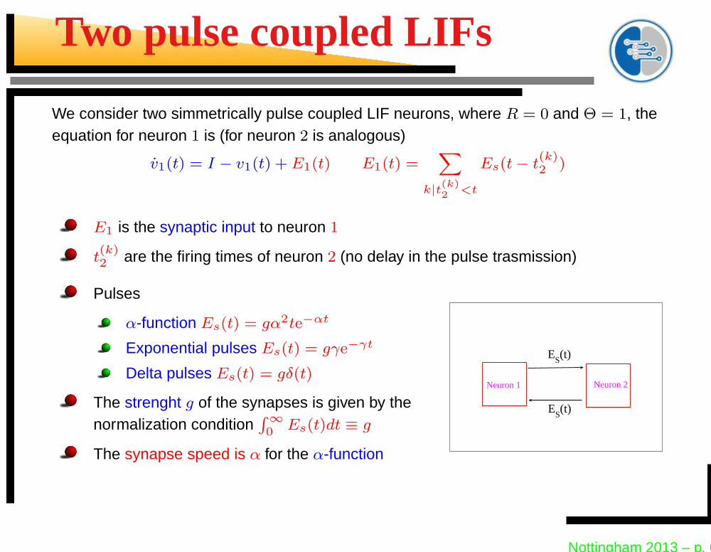
Two pulse coupled LIFs

We consider two simmetrically pulse coupled LIF neurons, where R = 0 and Θ = 1, theequation for neuron 1 is (for neuron 2 is analogous)

v1(t) = I − v1(t) + E1(t) E1(t) =X

k|t(k)2 <t

Es(t − t(k)2 )

E1 is the synaptic input to neuron 1

t(k)2 are the firing times of neuron 2 (no delay in the pulse trasmission)

Pulses

α-function Es(t) = gα2te−αt

Exponential pulses Es(t) = gγe−γt

Delta pulses Es(t) = gδ(t)

The strenght g of the synapses is given by thenormalization condition

R ∞0 Es(t)dt ≡ g

The synapse speed is α for the α-function

Neuron 1 Neuron 2

ES(t)

ES(t)


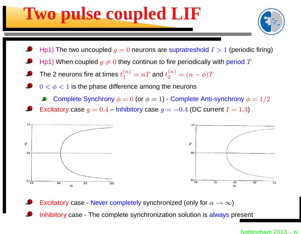
Two pulse coupled LIF

Hp1) The two uncoupled g = 0 neurons are supratreshold I > 1 (periodic firing)

Hp1) When coupled g 6= 0 they continue to fire periodically with period T

The 2 neurons fire at times t(n)1 = nT and t

(n)2 = (n − φ)T

0 < φ < 1 is the phase difference among the neurons

Complete Synchrony φ = 0 (or φ = 1) - Complete Anti-synchrony φ = 1/2

Excitatory case g = 0.4 – Inhibitory case g = −0.4 (DC current I = 1.3)

Excitatory case - Never completely synchronized (only for α → ∞)

Inhibitory case - The complete synchronization solution is always present


Theoretical explanation

Neuron 1 fires at times t(n)1 = nT with n = −∞, . . . ,−2,−1, 0

The synaptic input to neuron 2 at time t = θT with 0 < θ < 1 is the sum of all thepulses received in the past

E2(θT ) = ET (θ) =

0X

n=−∞

ES(θT − nT )

For α-fuctions the sum gives

ET (θ) =gα2T e−αθT

ˆ

θ(1 − e−αT ) + e−αT˜

(1 − e−αT )2

ET is periodic outside the interval ]0 : 1[

Neuron 2 fires at times t(n)2 = (n − φ)T – The synaptic input to neuron 1 is

E1(θT ) =

0X

n=−∞

ES(θT − nT + φ) = ET (θ + φ)


Theoretical explanation

Neuron 1 fires at time t = 0 =⇒ x1(0+) = 0

At time T the neuron 1 reaches again threshold therefore

x1(T ) = I(1 − e−T ) + T e−T

Z 1

0dθeθT ET (θ + φ) = 1

Neuron 2 fires at time t = −φT and after a period T it is again at threshold

x2((1 − φ)T ) = I(1 − e−T ) + T e−T

Z 1

0dθeθT ET (θ − φ) = 1

From the two above equations one can obtain the period T0 and the phase φ0

By combining the two equations above

G(φ) =x1(T ) − x2[(1 − φ)T ]

T= e−T

Z 1

0dθeθT [ET (θ + φ) − ET (θ − φ)]

If φ ≡ φ0 and T ≡ T0 then G(φ0) ≡ 0, possible solutions are

φ0 = 0 and φ0 = 1/2 since ET (θ + 1/2) = ET (θ − 1/2)


Stability of the solutions

Any solution φ0 is stable whenever G′(φ0) > 0

One can notice thatx2[(1 − φ)T ] = 1 − TG(φ)

if φ ≡ φ0 and T ≡ T0 then x2[(1 − φ0)T0] ≡ 1, since G(φ0) = 0

If the phase is perturbed φ = φ0 + δφ the neuron 2 will fire at time

t(n)2 = (n − φ)T0 = (n − φ0)T0 − (δφ)T0

since the solution is stable, the neuron to maintain constant the period T0 will firenext time at

tn+12 = (n + 1 − φ0)T0 + (δφ)T0 = (n + 1 − φ)T0 + 2(δφ)T0

Therefore at time t = (1 − φ)T0 the neuron has not reache the threshold

x2[(1 − φ)T ] < 1 =⇒ G(φ) ≃ G(φ0) + G′(φ0)δφ > 0 =⇒ G′(φ0) > 0


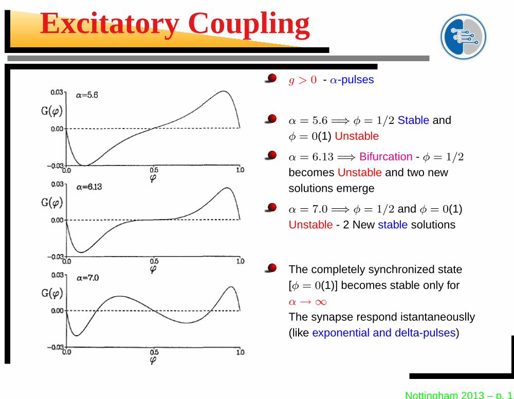
Excitatory Coupling

g > 0 - α-pulses

α = 5.6 =⇒ φ = 1/2 Stable andφ = 0(1) Unstable

α = 6.13 =⇒ Bifurcation - φ = 1/2

becomes Unstable and two newsolutions emerge

α = 7.0 =⇒ φ = 1/2 and φ = 0(1)Unstable - 2 New stable solutions

The completely synchronized state[φ = 0(1)] becomes stable only forα → ∞The synapse respond istantaneouslly(like exponential and delta-pulses)


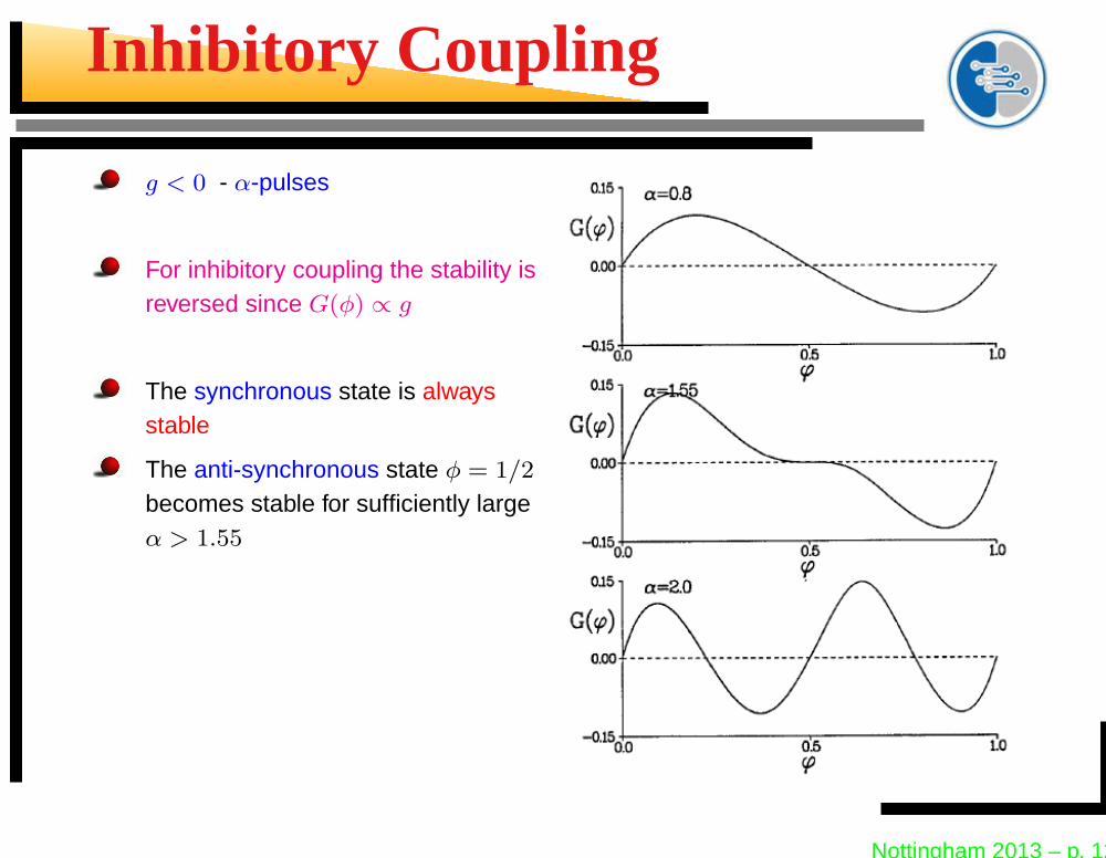
Inhibitory Coupling

g < 0 - α-pulses

For inhibitory coupling the stability isreversed since G(φ) ∝ g

The synchronous state is alwaysstable

The anti-synchronous state φ = 1/2

becomes stable for sufficiently largeα > 1.55


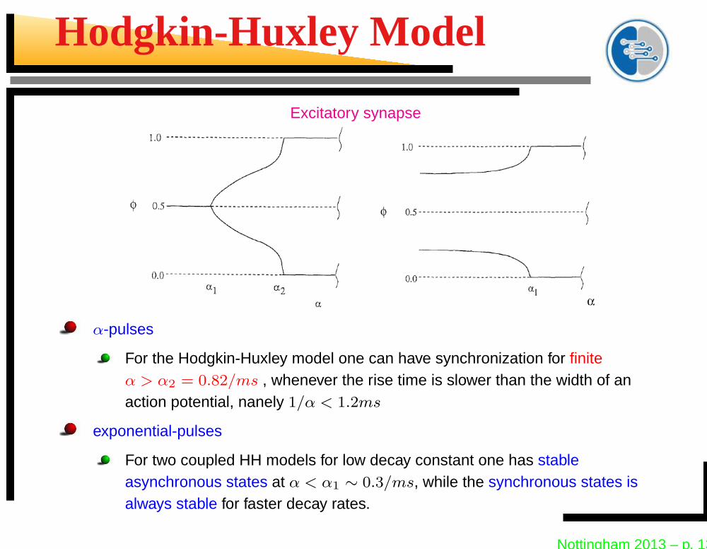
Hodgkin-Huxley Model

Excitatory synapse

α-pulses

For the Hodgkin-Huxley model one can have synchronization for finiteα > α2 = 0.82/ms , whenever the rise time is slower than the width of anaction potential, nanely 1/α < 1.2ms

exponential-pulses

For two coupled HH models for low decay constant one has stableasynchronous states at α < α1 ∼ 0.3/ms, while the synchronous states isalways stable for faster decay rates.


Conclusions

To summarize the results presented so far for the LIF model

g > 0

the synchronous state is stable only for extremely rapid synaptic response(namely, α = ∞) : like exponential or delta functions

the anti-synchronous state is stable for slow synapses α < αc

g < 0

the synchronous state is always stable apart for extremely rapid synapses

the anti-synchronous state is stable for fast synapses α > 1.55

In general excitation is desynchronizing for neurons with a response of Type I and forneuron of Type II (Hodgkin-Huxley) whenever the synaptic response is sufficiently slow

Type I : the arrival of an EPSP always advances the next firing time

Type II : the arrival of an EPSP just after the refractory period delays the nextfiring, while a EPSP received at a later time advances the next firing time

[Van Vreeswijk, Abbott, Ermentout, JCN (1994);Hansel, Mato, Meunier, Neural computation (1995)]


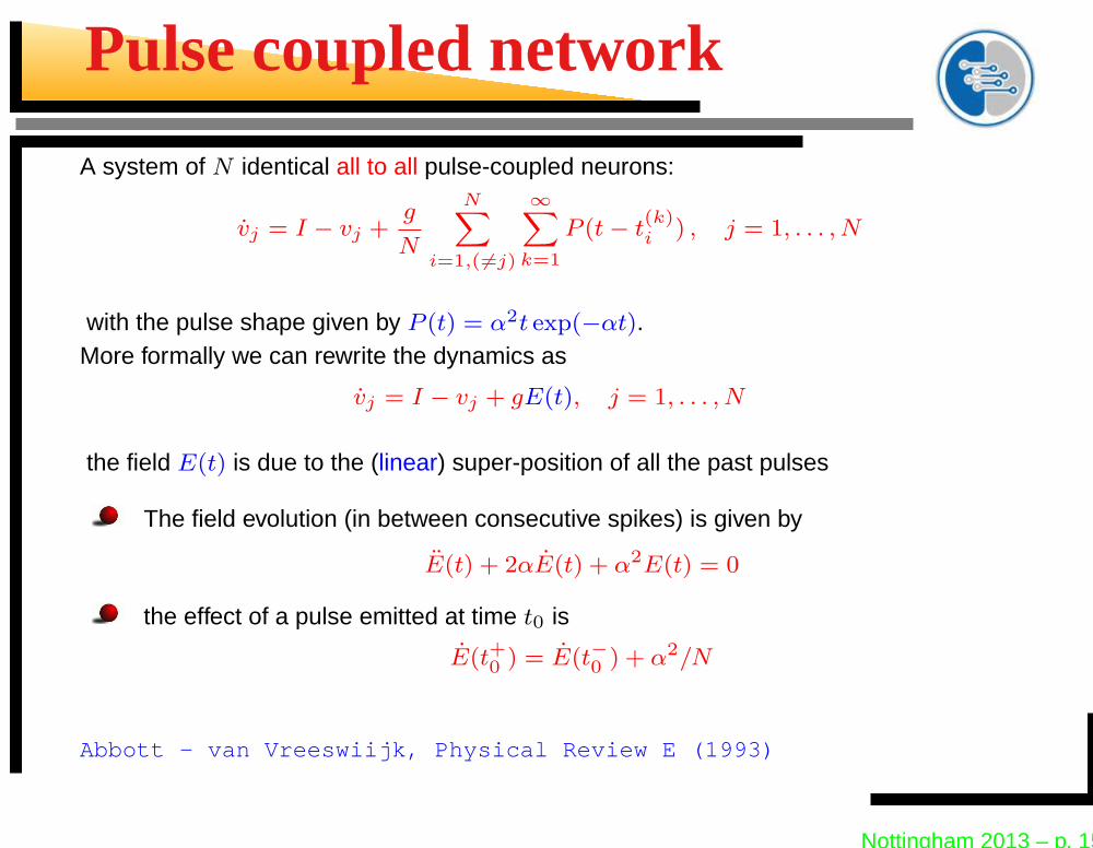
Pulse coupled network

A system of N identical all to all pulse-coupled neurons:

vj = I − vj +g

N

NX

i=1,( 6=j)

∞X

k=1

P (t − t(k)i ) , j = 1, . . . , N

with the pulse shape given by P (t) = α2t exp(−αt).More formally we can rewrite the dynamics as

vj = I − vj + gE(t), j = 1, . . . , N

the field E(t) is due to the (linear) super-position of all the past pulses

The field evolution (in between consecutive spikes) is given by

E(t) + 2αE(t) + α2E(t) = 0

the effect of a pulse emitted at time t0 is

E(t+0 ) = E(t−0 ) + α2/N

Abbott - van Vreeswiijk, Physical Review E (1993)


Fully coupled network

0 1 2time

0

5

10

F(t)

α=3 α=30

F(t) = α2 t e

-αt

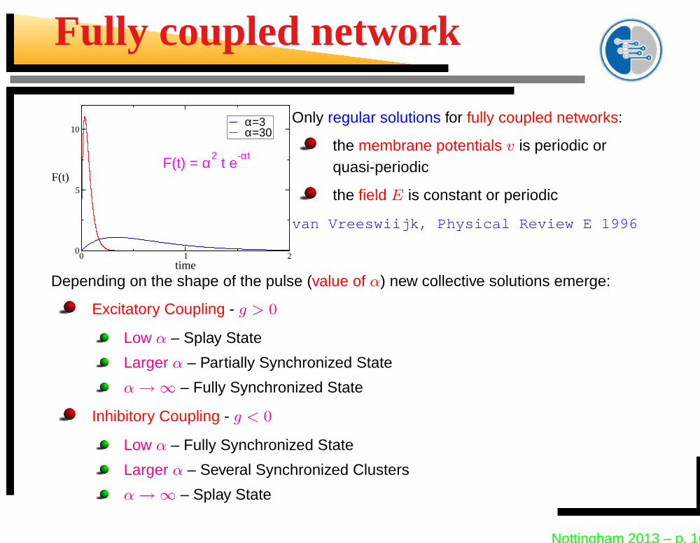
Only regular solutions for fully coupled networks:

the membrane potentials v is periodic orquasi-periodic

the field E is constant or periodic

van Vreeswiijk, Physical Review E 1996

Depending on the shape of the pulse (value of α) new collective solutions emerge:

Excitatory Coupling - g > 0

Low α – Splay State

Larger α – Partially Synchronized State

α → ∞ – Fully Synchronized State

Inhibitory Coupling - g < 0

Low α – Fully Synchronized State

Larger α – Several Synchronized Clusters

α → ∞ – Splay State


Splay States

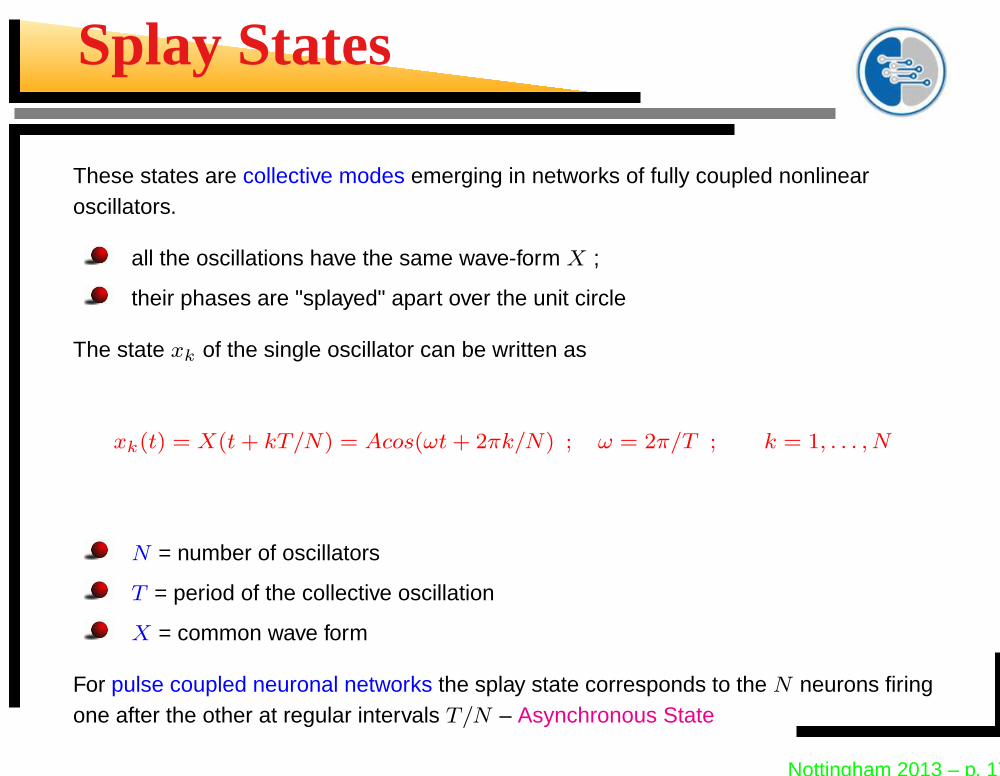
These states are collective modes emerging in networks of fully coupled nonlinearoscillators.

all the oscillations have the same wave-form X ;

their phases are "splayed" apart over the unit circle

The state xk of the single oscillator can be written as

xk(t) = X(t + kT/N) = Acos(ωt + 2πk/N) ; ω = 2π/T ; k = 1, . . . , N

N = number of oscillators

T = period of the collective oscillation

X = common wave form

For pulse coupled neuronal networks the splay state corresponds to the N neurons firingone after the other at regular intervals T/N – Asynchronous State


Splay States

Splay states have been numerically and theoretically studied in

Josephson junctions array (Strogatz-Mirollo, PRE , 1993)

globally coupled Ginzburg-Landau equations (Hakim-Rappel, PRE, 1992)

globally coupled laser model (Rappel, PRE, 1994)

fully pulse-coupled neuronal networks (Abbott-van Vreesvijk, PRE, 1993)

Splay states have been observed experimentally in

multimode laser systems (Wiesenfeld et al., PRL, 1990)

electronic circuits (Ashwin et al., Nonlinearity, 1990)

Nowdays Relevance for Neural Networks

LIF + Dynamic Synapses - Plasticity (Bressloff, PRE, 1999)

More realistic neuronal models (Brunel-Hansel, Neural Comp., 2006)


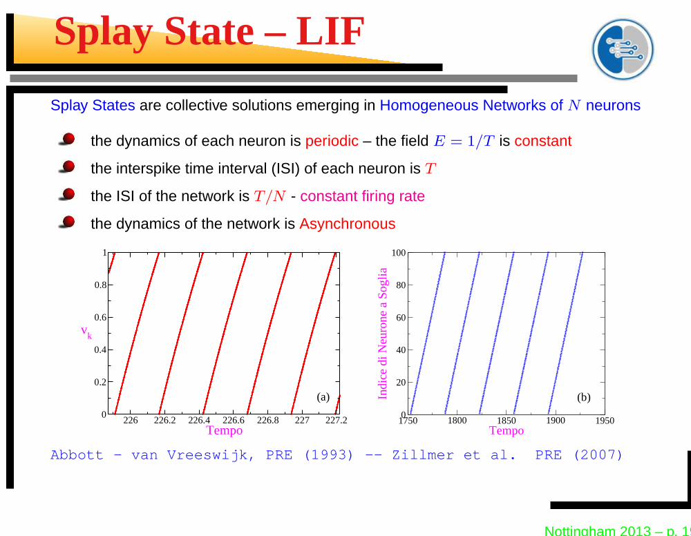
Splay State – LIF

Splay States are collective solutions emerging in Homogeneous Networks of N neurons

the dynamics of each neuron is periodic – the field E = 1/T is constant

the interspike time interval (ISI) of each neuron is T

the ISI of the network is T/N - constant firing rate

the dynamics of the network is Asynchronous

226 226.2 226.4 226.6 226.8 227 227.2Tempo

0

0.2

0.4

0.6

0.8

1

vk

(a)

1750 1800 1850 1900 1950Tempo

0

20

40

60

80

100

Indi

ce d

i Neu

rone

a S

oglia

(b)

Abbott - van Vreeswijk, PRE (1993) -- Zillmer et al. PRE (2007)


Splay state - LIF

In this framework, the periodic splay state reduces to the following fixed point:

τ(n) ≡ T

N

E(n) ≡ E , Q(n) ≡ Q

xj−1 = xje−T/N + 1 − x1e−T/N

where T is the time between two consecutive spike emissions of the same neuron.

A simple calculation yields,

Q =α2

N2

“

1 − e−αT/N”−1

, E = TQ“

eαT/N − 1”−1

.

and the period at the leading order (N ≫ 1 ) is given by

T = ln

»

aT + g

(a − 1)T + g

–


Partial Synchronization

0 0.2 0.4 0.6 0.8 1g

0

50

100

150

200

α

Partial Synchronization

Splay State

Partial Synchronization is a collective dynamics emerging in Excitatory HomogeneousNetworks for sufficiently narrow pulses

the dynamics of each neuron is quasi periodic - two frequencies

the firing rate of the network and the field E(t) are periodic

the quasi-periodic motions of the single neurons are arranged(quasi-synchronized) in such a way to give rise to a collective periodic field E(t)

van Vreeswiijk, PRE (1996) - Mohanty, Politi EPL (2006)


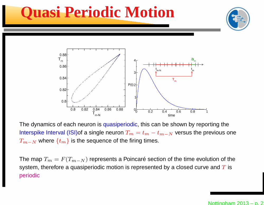
Quasi Periodic Motion

0 0.2 0.4 0.6 0.8 1time

0

1

2

3

4

P(t)

tmtm-N

Tm

δtm

The dynamics of each neuron is quasiperiodic, this can be shown by reporting theInterspike Interval (ISI)of a single neuron Tm = tm − tm−N versus the previous oneTm−N where {tm} is the sequence of the firing times.

The map Tm = F (Tm−N ) represents a Poincaré section of the time evolution of thesystem, therefore a quasiperiodic motion is represented by a closed curve and T isperiodic


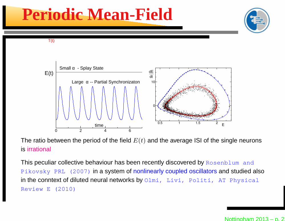
Periodic Mean-Field

0 2 4 6time

E(t)

T(t)

Small α - Splay State

Large α -- Partial Synchronizaton

The ratio between the period of the field E(t) and the average ISI of the single neuronsis irrational

This peculiar collective behaviour has been recently discovered by Rosenblum and

Pikovsky PRL (2007) in a system of nonlinearly coupled oscillators and studied alsoin the conntext of diluted neural networks by Olmi, Livi, Politi, AT Physical

Review E (2010)


Splay vs Partial Synchronization

The Splay State is Asynchronous

Partially Synchronized exhibit collective dynamics

0 1000 2000 3000t

0

0.2

0.4

0.6

0.8

1

E

0 2 4t

00.20.40.60.8

1

E

0 1000 2000 3000t

-1

0

1Rx10

7

0 1 2 3 4t

0.61

0.62

0.63

R

(a) (b)

(c) (d)


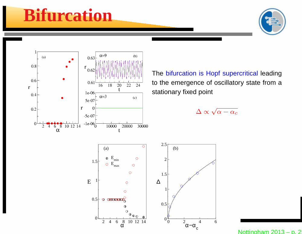
Bifurcation

The bifurcation is Hopf supercritical leadingto the emergence of oscillatory state from astationary fixed point

∆ ∝√

α − αc

2 4 6 8 10 12 14α

0

0.5

1

1.5

E

Emin

Emax

0 2 4 6α−αc

0

0.5

1

1.5

2

2.5

∆

(a) (b)


Documents

Coherent activity in excitatory neural networksâ€™