Embed Size (px)
Citation preview
Coase meets Tarski: New Insights from Coase’sTheory of the Firm∗
Tomoo Kikuchi†, Kazuo Nishimura‡ and John Stachurski§
August 28, 2012
Abstract
This paper formulates a model embedding the key ideas from Ronald Coase’s famousessay on the theory of the firm in a simple competitive equilibrium setting with anarbitrary number of firms. The model studies the structure of production when trans-action costs and diminishing returns to management are treated as given. In additionto recovering Coase’s main insights as equilibrium conditions, the model yields manynew predictions on prices, firm boundaries and division of the value chain.
Keywords: Transaction costs, vertical integration, production chainsJEL Classification: D02, D21, L11, L23
1 Introduction
Reflecting on a conversation with an ex-Soviet official wishing to know who was in chargeof supplying bread to the city of London, Seabright (2010) observed that “there was noth-ing naive about his question, because the answer ‘nobody is in charge’ is, when one thinks
∗The authors are indebted to Chris Jones, Takashi Kamihigashi, Pedro Gomis Porqueras and MakotoYano for helpful comments and discussions, and to Alex Olssen for excellent research assistance.
†Department of Economics, National University of Singapore. [email protected]‡Institute of Economic Research, Kyoto University. [email protected]§(Corresponding author) Research School of Economics, The Australian National University.
about it, astonishingly hard to believe.” Indeed, the ability of market forces to coordinatemany specialized activities and channel their collective output into the final goods de-manded by consumers has fascinated economists for centuries. In considering this phe-nomenon in his celebrated essay on the nature of the firm, Ronald Coase (1937) pushedthe analysis in a striking new direction: Given the efficiency of market coordination, com-bined with the fact that planned interactions within firms can, at least in principle, alsobe coordinated through the market, why, asked Coase, do firms exist at all? What need isthere for these “islands of conscious power in the ocean of unconscious cooperation”?1
These islands may be vast or small. For example, in 2011, Royal Dutch Shell operatedin over 80 countries, had annual revenue exceeding the GDP of 150 nations, and paidits CEO 35 times more than the president of the United States. In the same year, thetotal number of employees at Wal Mart exceeded the population of all but 4 US cities. Inaddition to such giants, tens of millions of smaller firms operate around the world.2 Whataccounts for the existence of the giant firms, and the multitude of smaller ones? Whatforces shape their individual sizes and their distribution? And if the market provides anefficient substitute for intra-firm coordination, then why are some CEO salaries measuredin tens of millions?
The modern approach to understanding these phenomena begins with Coase (1937), whosought to provide a theory of the firm that was both realistic and tractable “by two ofthe most powerful instruments of economic analysis developed by Marshall: the idea ofmargin and that of substitution, together giving the idea of substitution at the margin.”He argued that for firms to exist there must be costs associated with using the market (i.e.,transaction costs), and that entrepreneurs and managers must be able to substitute awayfrom the market by coordinating production at a lower cost within the firm. On the otherhand, since firms do not expand without limit, a countervailing force must be present.Coase referred to this force as “diminishing returns to management.” The boundary of thefirm is then determined by the point at which the cost of organizing another productivetask within the firm is equal to the cost of acquiring a similar input through the market.
Subsequent to Coase’s analysis, many economists have expanded on and developed thetheory of the firm. Researchers have considered the effect of imperfect information, in-centive and agency problems, incomplete contracts, property rights, decision rights, andthe microfoundations of transaction costs. Major contributions were made by Jensen andMeckling (1976), Williamson (1979, 1981), Klein, Crawford and Alchian (1978), Gross-man and Hart (1986), Hart and Moore (1990), Holmstrom and Milgrom (1994), Grossmanand Helpman (2002) and many others. These studies have been immensely valuable inbuilding an understanding of different attributes and functions of the firm. Up to datesurveys and references can be found in Aghion and Holden (2011) and Bresnahan and
1This phrase from Coase’s essay is originally due to Robertson (1923).2Sources: United States Census Bureau and the Forbes Global 2000 List.
2
Levin (2012).
In this paper our objective is different. Rather than extending or critiquing the underly-ing ideas in Coase’s theory, our aim is to show that Coase’s basic framework has a greatdeal more to give. We begin by embedding the essential features of his verbal analysis ina competitive model with transaction costs and an arbitrary number of firms. By fram-ing the choice problem of firms recursively, we reduce the model to a single functionalequation for equilibrium prices. We prove that this functional equation has a unique so-lution, and that this solution identifies a well-defined disintegration of the value chaincoordinated through the price system. The model recovers Coase’s original insights onthe boundaries of individual firms in the form of equations derived from first order con-ditions. More importantly, it also allows us to study the implications of Coase’s ideas forthe structure of production along the value chain, as determined by the interactions be-tween the choices of individual firms and the equilibrium set of prices. These interactionsresult in a set of additional predictions regarding the relationship between upstream anddownstream firms, the equilibrium impact of transaction and management costs and thedistribution of firms.
The first version of our model involves sequential production over a continuum of tasks.Economists have used this structure to address a variety of questions. Recent examplesinclude Grossman and Rossi-Hansberg (2008, 2012), Costinot (2009), Antras and Chor(2011) and Costinot, Vogel and Wang (2011). Perhaps the most similar to our paper isCostinot, Vogel and Wang (2011), which studies global supply chains. Their model isnonetheless different in that firms are heterogeneous, and that the production processesis affected by “mistakes.” In our model mistakes are absent, firms are ex ante identical,and all ex post heterogeneity is generated as part of the equilibrium. In addition, our ana-lytical techniques, based on recursive subdivision of tasks, give us a very detailed pictureof prices over the continuum, and allow us to consider such extensions as productionwith multiple upstream partners (section 4).
The rest of the paper is structured as follows. Section 2 describes the model. The equi-librium is analyzed in section 3. Section 4 considers possible extensions, while section 5looks at implications and predictions. Section 6 concludes.
2 The Model
Following Coase (1937), our focus is supply side and partial equilibrium. To start theanalysis we consider a single good that is produced through the sequential completion ofa large number of tasks. (More complex production structures are treated in section 4.)In order to provide a sharper marginal analysis, we model the processing stages as acontinuum from zero to one. For example, at stage 0.9 the good is 90% complete.
3
0 1t1
processed by firm 1subcontracted by firm 1 to firm 2
0 t1t2
subcontracted by 2 to 3 processed by firm 2
0 t2
processed by firm 3
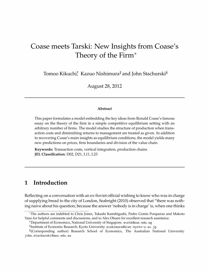
Figure 1: Disintegration of the value chain
t3 t0t1t2
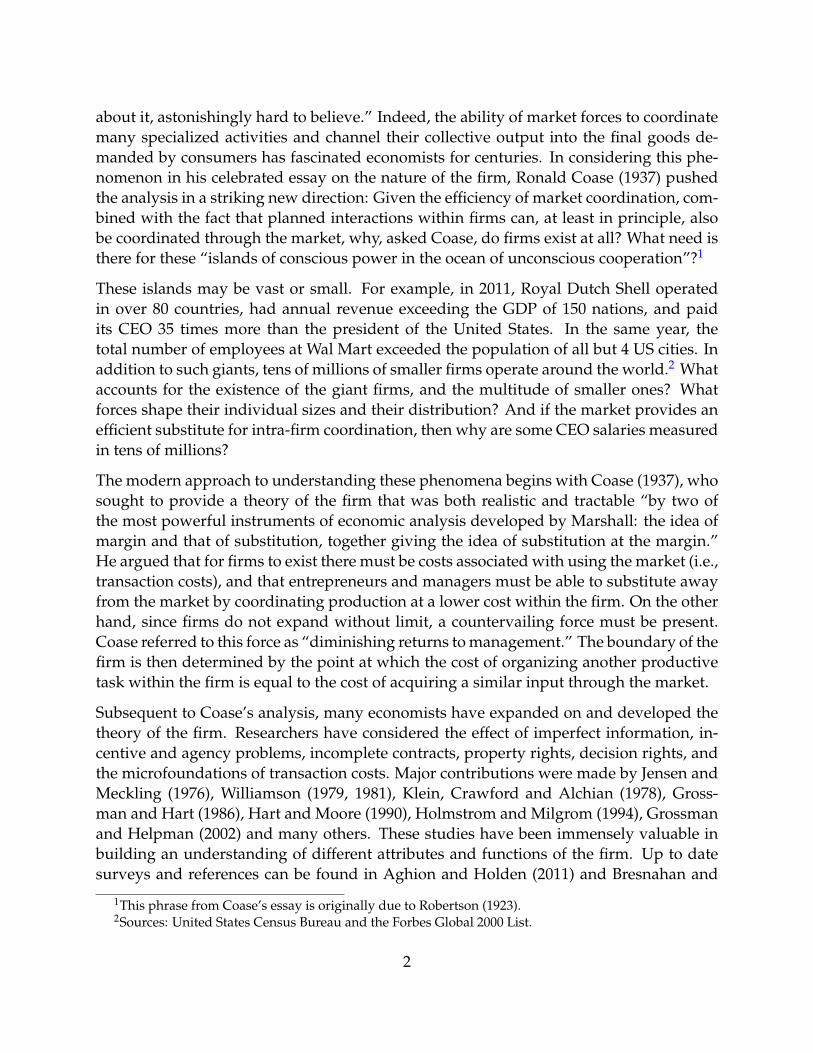
Step 1: contract formation from downstream to upstream
Step 2: production from upstream to downstream
Figure 2: Contracts and Production
2.1 The Production Chain
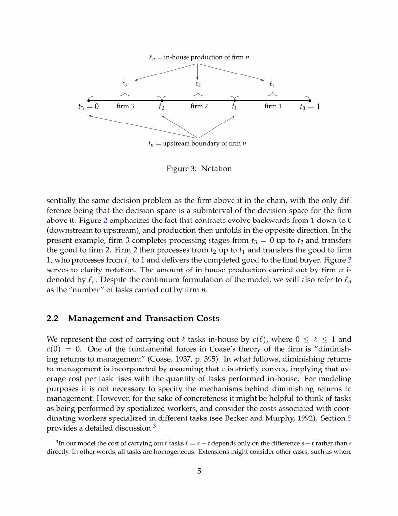
The processing stages are indexed by t ∈ [0, 1], with t = 0 indicating that no tasks havebeen undertaken and t = 1 indicating that production of one unit of the good is complete.Allocation of tasks between firms is determined by subcontracting. The subcontractingscheme is illustrated in figure 1. In this example, firm 1 receives a contract to sell oneunit of the completed good to a final buyer. Firm 1 then forms a contract with firm 2to purchase the good at processing stage t1. Firm 2 repeats this procedure, forming acontract with firm 3 to purchase the good at stage t2. In the example in figure 1, firm 3decides to complete the chain, selecting t3 = 0.
Figure 1 already suggests the recursive nature of the decision problem for each firm. Inchoosing how many processing stages to subcontract, each successive firm will face es-
4
t3 = 0 t0 = 1t1t2
`3 `2 `1
firm 1firm 2firm 3
`n = in-house production of firm n
tn = upstream boundary of firm n
Figure 3: Notation
sentially the same decision problem as the firm above it in the chain, with the only dif-ference being that the decision space is a subinterval of the decision space for the firmabove it. Figure 2 emphasizes the fact that contracts evolve backwards from 1 down to 0(downstream to upstream), and production then unfolds in the opposite direction. In thepresent example, firm 3 completes processing stages from t3 = 0 up to t2 and transfersthe good to firm 2. Firm 2 then processes from t2 up to t1 and transfers the good to firm1, who processes from t1 to 1 and delivers the completed good to the final buyer. Figure 3serves to clarify notation. The amount of in-house production carried out by firm n isdenoted by `n. Despite the continuum formulation of the model, we will also refer to `nas the “number” of tasks carried out by firm n.
2.2 Management and Transaction Costs
We represent the cost of carrying out ` tasks in-house by c(`), where 0 ≤ ` ≤ 1 andc(0) = 0. One of the fundamental forces in Coase’s theory of the firm is “diminish-ing returns to management” (Coase, 1937, p. 395). In what follows, diminishing returnsto management is incorporated by assuming that c is strictly convex, implying that av-erage cost per task rises with the quantity of tasks performed in-house. For modelingpurposes it is not necessary to specify the mechanisms behind diminishing returns tomanagement. However, for the sake of concreteness it might be helpful to think of tasksas being performed by specialized workers, and consider the costs associated with coor-dinating workers specialized in different tasks (see Becker and Murphy, 1992). Section 5provides a detailed discussion.3
3In our model the cost of carrying out ` tasks ` = s− t depends only on the difference s− t rather than sdirectly. In other words, all tasks are homogeneous. Extensions might consider other cases, such as where
5
Diminishing returns to management favors sourcing inputs externally over in-house pro-duction. Absent a countervailing force, the “equilibrium” size of firms may be infintes-imally small. In Coase’s analysis, the countervailing force is provided by market trans-action costs. Section 5 gives a detailed discussion of transaction costs. An important ex-ample is the cost of negotiating, monitoring and enforcing contracts with suppliers (thinkof complete but costly contracts). For now we follow Arrow (1969) by simply regardingtransaction costs as a wedge between the buyer’s and seller’s prices. As will be shownin section 4.1, it matters little from a qualitative perspective whether the transaction costis borne by the buyer, the seller or both. Hence we assume that the cost is borne only bythe buyer. In particular, when the partially processed good is purchased at price p, thebuyer’s total outlay is equal to δp with δ > 1. The transaction cost (δ − 1)p is paid toagents outside the model.
Collect all assumptions on δ and c together, we assume that δ > 1 and c is strictly convexand continuously differentiable with c(0) = 0, c′(0) > 0 and δc′(0) ≤ c′(1). The last twoconditions are only mildly restrictive and yield tight characterizations of the equilibrium.Since c is convex and c′(0) > 0, the function c is strictly increasing.
2.3 Profit Maximization
We assume that all firms are ex ante identical and act as price takers. Contracts are com-plete, information is perfect, and active firms are surrounded by an infinite number ofcompetitive firms ready to step in on either the buyer or the seller side should it be prof-itable to do so. There are no fixed costs or barriers to entry. As a result, no holdup occursin our model.
Let p(t) represent the price of the good completed up to stage t. (In particular, p(1) is theprice of the final completed good.) To begin the process of determining prices, considera firm that enters a contract to supply the good at stage s ∈ (0, 1], and purchase the goodat stage t ≤ s. The firm undertakes the remaining ` = s− t tasks in house, and its totalcosts are given by the sum of its processing costs c(s− t) and the gross input cost δp(t).Recalling that transaction costs are paid only by the buyer, profits are p(s) − c(s − t) −δp(t). If t is chosen to minimize costs, then profits become
π(s) = p(s)−mint≤s{δp(t) + c(s− t)}. (1)
Here and below, the restriction 0 ≤ t in the minimum is understood.
upstream tasks are more routine and hence cheaper. Here our interest is in equilibrium prices and choicesof firms in the base case where tasks are ex-ante identical.
6
3 Equilibrium
The model can now be closed by a zero profit and boundary condition. This sectiondescribes equilibrium prices and the resulting vertical production structure.
3.1 Equilibrium Prices
Competition forces firm profits to zero, implying that π(s) in (1) equals zero for all s ∈(0, 1]. This places a restriction on p(s) for s ∈ (0, 1]. The remaining value p(0) can beregarded as the revenue of firms that supply the initial inputs to production. We imposea zero profits condition in this sector as well, implying that p(0) is equal to the cost ofproducing these inputs. To simplify notation, we assume that this cost is zero, and hencethe boundary condition is p(0) = 0. Formally, we say that a function p : [0, 1] → R+
satisfies the equilibrium price equation if
p(s) = inft≤s{δp(t) + c(s− t)} for all s ∈ [0, 1]. (2)
Evidently the zero function is a solution to the equilibrium price equation. A nonzerosolution p∗ to the equilibrium price equation is called an equilibrium price function. Ex-istence of an equilibrium price function can be established via the Knaster-Tarski fixedpoint theorem. To see this, let P be the set of functions p from [0, 1] to R such thatc′(0)s ≤ p(s) ≤ c(s) for all 0 ≤ s ≤ 1, and let T be the operator defined over p ∈P by
Tp(s) = inft≤s{δp(t) + c(s− t)} for all s ∈ [0, 1]. (3)
It is not hard to verify that T maps P into itself (see lemma 7.1 in section 7.2). As c′(0)is assumed to be strictly positive, no element of P is the zero function, and hence anyfixed point of T is a (nontrivial) equilibrium price function. While T is not a contractionmapping in any obvious metric, it is monotone increasing on P (i.e., order preserving)when P is endowed with the usual partial order (p ≤ q if p(s) ≤ q(s) for all s) because ifp ≤ q, then for any s ∈ [0, 1] we have inft≤s {δp(t) + c(s− t)} ≤ inft≤s {δq(t) + c(s− t)},and hence Tp(s) ≤ Tq(s). Since P is a complete lattice, the Knaster-Tarski fixed pointtheorem ensures the existence of a fixed point in P .
Although the proceeding argument yields existence of an equilibrium price function p∗,we also wish to know whether the solution is unique over some suitable class of functions,what properties it possesses, and if numerical methods can be found to compute it in aconsistent fashion. An equally important question is whether or not, given the solution,production is actually realized. In particular, given the pricing function, it is conceivablethat, in the manner of Zeno’s paradox, the backwards contracting problem never termi-nates. For example, if firm i implements `i = 2−i tasks for all i, then the (n + 1)-th firm
7
contracts at stage tn = 1 − ∑ni=1 `i = 2−n. Since this value is always strictly positive,
no termination occurs in finite time. Such behavior must be ruled out in order to verifyexistence of a realistic equilibrium.
Regarding the set P , the upper and lower bound functions s 7→ c(s) and s 7→ c′(0)sdefining P have a natural interpretation as representing prices when transaction costs arevery high and very low respectively. Regarding the upper bound function, it is intuitivethat if δ is very large, then transaction costs will be prohibitively expensive and a singlefirm will implement the whole process in-house. Their cost at stage s will be c(s). Givenzero profits this is equal to the price p(s). Thus, the upper bound function represents theprice when transaction costs are very large and only one firm operates. On the other hand,as δ ↓ 1, strict positivity of c will cause the number of firms to increase without limit, andthe amount of in-house production ` at each firm will decrease to zero. Average costs ateach firm will be c(`)/`→ c′(0), and the price at stage s will be the integral c′(0)s. Hencethe lower bound function represents the price when transaction costs are arbitrarily low.
3.2 Properties of the Solution
Our first result on properties of the solution establishes uniqueness of the equilibriumprice function given the two primitives c and δ, and shows that the price function isalways strictly convex and continuously differentiable. (Here and below, proofs are de-ferred until section 7.) In the statement of the next theorem, P0 is defined to be the set offunctions in P that are convex and K-Lipschitz for K := c′(1).4 Also, given an equilib-rium price function p∗, we let the optimal choices be defined by
t∗(s) := arg mint≤s
{δp∗(t) + c(s− t)} and `∗(s) := s− t∗(s), (4)
For example, `∗(s) is the optimal amount of in-house production for a firm that is con-tracted to deliver the good at stage s.
Theorem 3.1. The equilibrium pricing equation has a unique solution in P0. The solution p∗ isstrictly convex, strictly increasing and continuously differentiable, with
(p∗)′(s) = c′(`∗(s)) for all s ∈ (0, 1). (5)
Moreover, the functions t∗ and `∗ are well-defined and single-valued on [0, 1]. Both are increasingand K-Lipschitz with K := 1.
The first order condition for (4) is
δ(p∗)′(t∗(s)) = c′(s− t∗(s)). (6)
4F : X → R is called K-Lipschitz if |F(a)− F(b)| ≤ K|a− b| for any a, b ∈ X.
8
0.0 0.2 0.4 0.6 0.8 1.00
5
10
15
20
25
30
35δ=1.05
δ=1.15
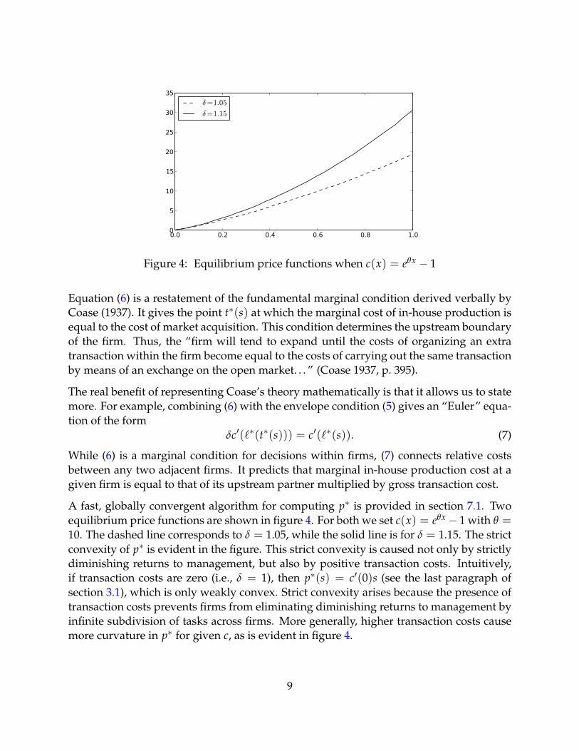
Figure 4: Equilibrium price functions when c(x) = eθx − 1
Equation (6) is a restatement of the fundamental marginal condition derived verbally byCoase (1937). It gives the point t∗(s) at which the marginal cost of in-house production isequal to the cost of market acquisition. This condition determines the upstream boundaryof the firm. Thus, the “firm will tend to expand until the costs of organizing an extratransaction within the firm become equal to the costs of carrying out the same transactionby means of an exchange on the open market. . . ” (Coase 1937, p. 395).
The real benefit of representing Coase’s theory mathematically is that it allows us to statemore. For example, combining (6) with the envelope condition (5) gives an “Euler” equa-tion of the form
δc′(`∗(t∗(s))) = c′(`∗(s)). (7)
While (6) is a marginal condition for decisions within firms, (7) connects relative costsbetween any two adjacent firms. It predicts that marginal in-house production cost at agiven firm is equal to that of its upstream partner multiplied by gross transaction cost.
A fast, globally convergent algorithm for computing p∗ is provided in section 7.1. Twoequilibrium price functions are shown in figure 4. For both we set c(x) = eθx− 1 with θ =10. The dashed line corresponds to δ = 1.05, while the solid line is for δ = 1.15. The strictconvexity of p∗ is evident in the figure. This strict convexity is caused not only by strictlydiminishing returns to management, but also by positive transaction costs. Intuitively,if transaction costs are zero (i.e., δ = 1), then p∗(s) = c′(0)s (see the last paragraph ofsection 3.1), which is only weakly convex. Strict convexity arises because the presence oftransaction costs prevents firms from eliminating diminishing returns to management byinfinite subdivision of tasks across firms. More generally, higher transaction costs causemore curvature in p∗ for given c, as is evident in figure 4.
9
3.3 Structure of Production
Given the pricing function p∗, the equilibrium structure of the vertical production chainintroduced in figures 1–3 is determined recursively: Firm 1 receives the order for thefinal good at price p∗(1). Letting t∗ be as defined in (4), firm 1 subcontracts to firm 2 att1 := t∗(1), firm 2 subcontracts to firm 3 at t2 := t∗(t1), and, in general, firm n subcontractsto firm n + 1 at
tn := t∗(tn−1) with t0 = 1. (8)
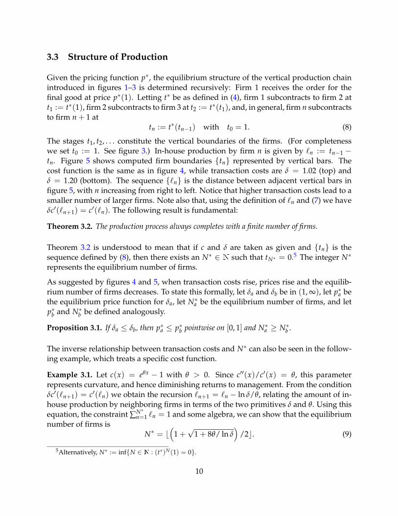
The stages t1, t2, . . . constitute the vertical boundaries of the firms. (For completenesswe set t0 := 1. See figure 3.) In-house production by firm n is given by `n := tn−1 −tn. Figure 5 shows computed firm boundaries {tn} represented by vertical bars. Thecost function is the same as in figure 4, while transaction costs are δ = 1.02 (top) andδ = 1.20 (bottom). The sequence {`n} is the distance between adjacent vertical bars infigure 5, with n increasing from right to left. Notice that higher transaction costs lead to asmaller number of larger firms. Note also that, using the definition of `n and (7) we haveδc′(`n+1) = c′(`n). The following result is fundamental:
Theorem 3.2. The production process always completes with a finite number of firms.
Theorem 3.2 is understood to mean that if c and δ are taken as given and {tn} is thesequence defined by (8), then there exists an N∗ ∈ N such that tN∗ = 0.5 The integer N∗
represents the equilibrium number of firms.
As suggested by figures 4 and 5, when transaction costs rise, prices rise and the equilib-rium number of firms decreases. To state this formally, let δa and δb be in (1, ∞), let p∗a bethe equilibrium price function for δa, let N∗a be the equilibrium number of firms, and letp∗b and N∗b be defined analogously.
Proposition 3.1. If δa ≤ δb, then p∗a ≤ p∗b pointwise on [0, 1] and N∗a ≥ N∗b .
The inverse relationship between transaction costs and N∗ can also be seen in the follow-ing example, which treats a specific cost function.
Example 3.1. Let c(x) = eθx − 1 with θ > 0. Since c′′(x)/c′(x) = θ, this parameterrepresents curvature, and hence diminishing returns to management. From the conditionδc′(`n+1) = c′(`n) we obtain the recursion `n+1 = `n − ln δ/θ, relating the amount of in-house production by neighboring firms in terms of the two primitives δ and θ. Using thisequation, the constraint ∑N∗
n=1 `n = 1 and some algebra, we can show that the equilibriumnumber of firms is
N∗ = b(
1 +√
1 + 8θ/ ln δ)
/2c. (9)
5Alternatively, N∗ := inf{N ∈ N : (t∗)N(1) = 0}.
10
0.0 0.2 0.4 0.6 0.8 1.002468
10121416
0.0 0.2 0.4 0.6 0.8 1.005
10152025303540
Figure 5: Firm boundaries for δ = 1.02 (top) and δ = 1.20 (bottom)
A proof is given in lemma 7.10 below. Here bac is the largest integer less than or equalto a. As expected, the number of firms is increasing in θ (more rapid diminishing returnsto management implies a larger number of relatively small firms, and greater use of themarket) and decreasing in δ (see figure 5).
Let vn := p∗(tn−1)− p∗(tn), the value added of firm n. The next results on prices and thestructure of production follow from theorems 3.1 and 3.2.
Proposition 3.2. p∗(1) = ∑N∗i=1 δi−1c(`i).
Proposition 3.3. `n+1 ≤ `n and vn+1 ≤ vn for all n in 1, . . . , N∗ − 1.
Proposition 3.2 confirms that in equilibrium the price of the final good is the sum of costsincurred. Proposition 3.3 is more significant. It states that the number of tasks performedin-house is larger the further downstream the firm is in the value chain (as can be seenin figure 5), and the same is true for the amount of value added each firm contributes tothe final value of the good. The increase in in-house production as we move downstreamis due to the fact that the value of the good increases as more processing stages are com-pleted, and with this increase comes a proportional rise in transaction costs (intuitively,more valuable goods entail more costly contracts). As a result, downstream firms facehigher transaction costs. To economize on these costs they produce more in-house. Thesecond inequality in proposition 3.3 follows from the first and convexity of p∗.
11

1 2 3 4 5 6 7log rank
14.4
14.2
14.0
13.8
13.6
13.4
13.2
13.0
log
valu
e ad
ded
Figure 6: Size-rank plot (logscale)
Proposition 3.3 indicates that, although firms are ex-ante identical, in equilibrium theywill organize into a nondegenerate distribution, with firm size measured by value addedincreasing from upstream to downstream. The shape of the distribution of firm sizes de-pends on the primitives c and δ. Typically it is right-skewed. The rank-size plot for firmsize measured by value added is shown in figure 6. Each point corresponds to one firmin the vertical structure generated by primitives c(x) = exp(x2) − 1 and δ = 1.00075.In equilibrium there are 1402 firms. The vertical axis is the log of value added, and thehorizontal axis is the log of firm rank by value added. (Firms are ranked from largest tosmallest in terms of value added.) The rank-size distribution shows significant curvature,although it is almost linear for smaller firms. (In fact, for these parameters, a linear re-gression of the data restricted to the smallest decile of firms has a very close fit and slopeof -1.02. A slope of -1 corresponds to Zipf’s law.)
4 Extensions
4.1 Alternative Costs
Until now we have assumed that the transaction cost is borne entirely by the buyer, whileclaiming that this assumption costs little in terms of generality. To see why, supposeinstead that the transaction cost is borne by both the buyer and the seller in some givenproportions. (For example, the cost of drafting and negotiating contracts might be borneby both sides of the transaction.) In particular, suppose as before that when the buyerpurchases the good at price p(t) her total outlay is δp(t) with δ > 1, and suppose in
12
addition that the revenue net of contract costs received by the seller is γp(t) for some γ ∈(0, 1). The profit function in section 2.3 then becomes π(s, t) = γp(s)− c(s− t)− δp(t).Minimizing over t ≤ s and setting profits to zero yields
p(s) = mint≤s
{δ
γp(t) +
c(s− t)γ
}. (10)
This equation has the same form as (2). Since δ/γ > 1 and c/γ inherits from c all theproperties of the cost function stated in section 2.2, the preceding results go through, andqualitative properties of the solution are the same.
4.2 Multiple Partners
So far we have assumed that production is linearly sequential, and firms contract withonly one parter. In reality, most vertically integrated firms have multiple upstream part-ners. For example, in 2004 Toyota group had 168 direct parts suppliers. These primarysuppliers themselves had 5,437 direct suppliers, and in turn these secondary suppliershad 41,703 tertiary suppliers (Tsuji, 2004).
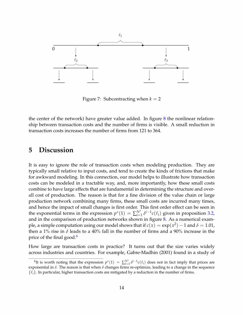
As a result of our solution strategy based on recursive subdivision of tasks, our modelcan easily be generalized to include multiple upstream partners. To begin, consider thetree in figure 7. As before, firm n choose an interval `n of tasks to perform in-house, andsubcontracts the remainder. In this case, however, each downstream firm subcontracts totwo upstream partners. We can also consider more general cases, where each downstreamfirm subcontracts has k upstream partners. If a firm contracts to supply the good at stages, chooses a quantity ` ≤ s to produce in-house, and then divides the remainder s − `equally across k upstream partners, then profits will be given by revenue p(s) minusinput costs δ k p((s− `)/k) minus in-house production costs c(`). That is,
π(s, `) = p(s)− δ k p((s− `)/k)− c(`).
Setting profits to zero, letting t := s− ` and minimizing with respect to t yields the func-tional equation
p(s) = inft≤s{δ k p(t/k) + c(s− t)}.
This equation is an immediate generalization of (2). Similar techniques can be employedto show the existence and uniqueness of a solution p∗, to compute p∗, and to computefrom p∗ the optimal choices of firms and the resulting distribution of firms.
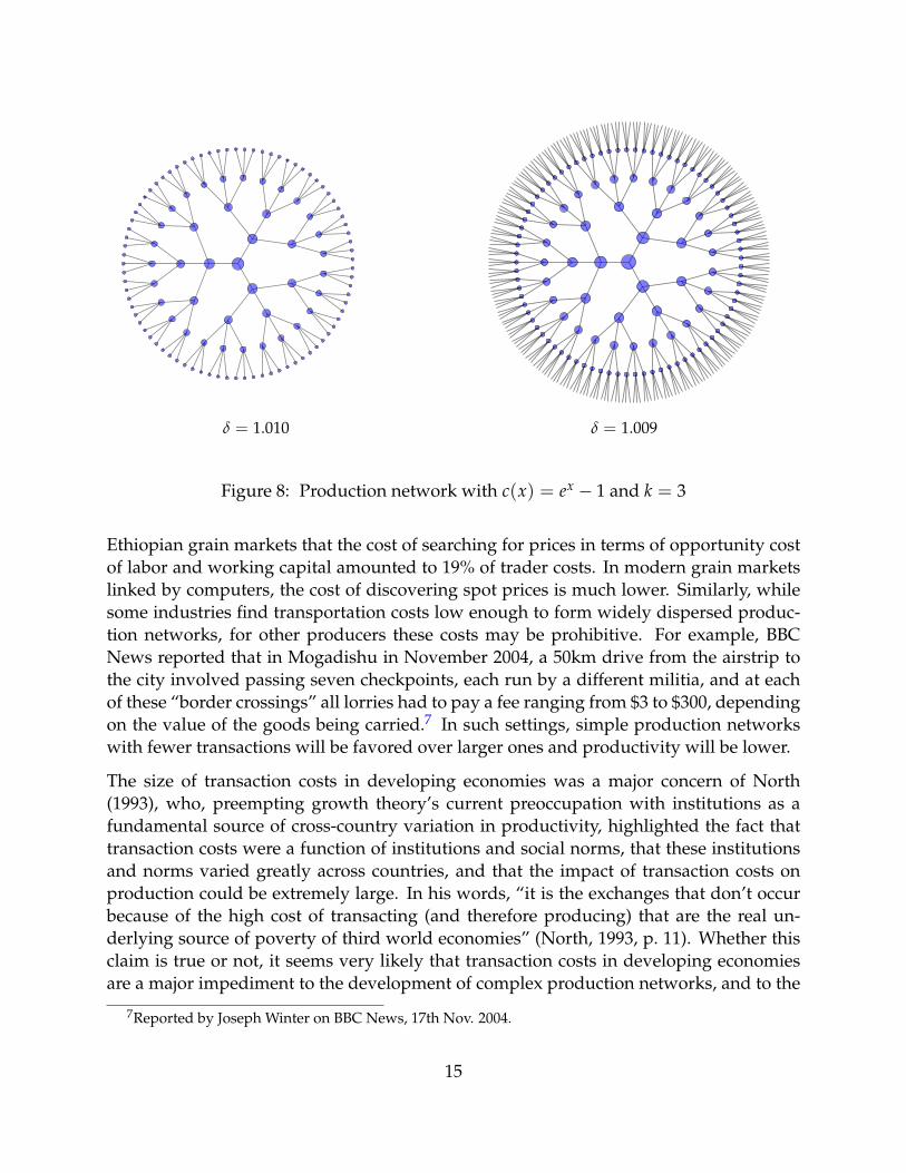
Figure 8 shows the results of these computations for k = 3 under two parameterizations.In these networks, each node represents a firm, and the node size is proportional to thevalue added of that firm. As with the k = 1 case, downstream firms (i.e., firms towards
13
0 1
`1
`2 `3
Figure 7: Subcontracting when k = 2
the center of the network) have greater value added. In figure 8 the nonlinear relation-ship between transaction costs and the number of firms is visible. A small reduction intransaction costs increases the number of firms from 121 to 364.
5 Discussion
It is easy to ignore the role of transaction costs when modeling production. They aretypically small relative to input costs, and tend to create the kinds of frictions that makefor awkward modeling. In this connection, our model helps to illustrate how transactioncosts can be modeled in a tractable way, and, more importantly, how these small costscombine to have large effects that are fundamental in determining the structure and over-all cost of production. The reason is that for a fine division of the value chain or largeproduction network combining many firms, these small costs are incurred many times,and hence the impact of small changes is first order. This first order effect can be seen inthe exponential terms in the expression p∗(1) = ∑N∗
i=1 δi−1c(`i) given in proposition 3.2,and in the comparison of production networks shown in figure 8. As a numerical exam-ple, a simple computation using our model shows that if c(x) = exp(x2)− 1 and δ = 1.01,then a 1% rise in δ leads to a 40% fall in the number of firms and a 90% increase in theprice of the final good.6
How large are transaction costs in practice? It turns out that the size varies widelyacross industries and countries. For example, Gabre-Madhin (2001) found in a study of
6It is worth noting that the expression p∗(1) = ∑N∗i=1 δi−1c(`i) does not in fact imply that prices are
exponential in δ. The reason is that when δ changes firms re-optimize, leading to a change in the sequence{`i}. In particular, higher transaction costs are mitigated by a reduction in the number of firms.
14
δ = 1.010 δ = 1.009
Figure 8: Production network with c(x) = ex − 1 and k = 3
Ethiopian grain markets that the cost of searching for prices in terms of opportunity costof labor and working capital amounted to 19% of trader costs. In modern grain marketslinked by computers, the cost of discovering spot prices is much lower. Similarly, whilesome industries find transportation costs low enough to form widely dispersed produc-tion networks, for other producers these costs may be prohibitive. For example, BBCNews reported that in Mogadishu in November 2004, a 50km drive from the airstrip tothe city involved passing seven checkpoints, each run by a different militia, and at eachof these “border crossings” all lorries had to pay a fee ranging from $3 to $300, dependingon the value of the goods being carried.7 In such settings, simple production networkswith fewer transactions will be favored over larger ones and productivity will be lower.
The size of transaction costs in developing economies was a major concern of North(1993), who, preempting growth theory’s current preoccupation with institutions as afundamental source of cross-country variation in productivity, highlighted the fact thattransaction costs were a function of institutions and social norms, that these institutionsand norms varied greatly across countries, and that the impact of transaction costs onproduction could be extremely large. In his words, “it is the exchanges that don’t occurbecause of the high cost of transacting (and therefore producing) that are the real un-derlying source of poverty of third world economies” (North, 1993, p. 11). Whether thisclaim is true or not, it seems very likely that transaction costs in developing economiesare a major impediment to the development of complex production networks, and to the
7Reported by Joseph Winter on BBC News, 17th Nov. 2004.
15
adoption of modern technologies that require such networks.
On a theoretical level, recognition of the systemic impact of transaction costs dates backto Adam Smith (1776). Smith famously argued that the division of labor is limited by theextent of the market. Pushing the analysis further, he also noted that the extent of themarket is itself limited by transportation costs (Smith, 1776, p. 31). This was an early ac-knowledgment of the fundamental role played by transaction costs in limiting the special-ization and the division of labor. Smith’s insights in this direction have been extended byauthors such as Houthakker (1956), Yang and Ng (1993) and Becker and Murphy (2002).Our model is clearly connected, although the modeling techniques are very different andthe focus is on division of tasks across firms.
The most commonly cited transaction costs include transportation and transaction fees,search, bargaining and information costs, costs of assessing credit worthiness and relia-bility, and the costs associated with negotiating, writing, monitoring and enforcing con-tracts. Discussion of these different costs can be found in references such as Coase (1937),Williamson (1979, 1981), Arrow (1969) and North (1993). Both Coase and North empha-sized contracts as a major component of transaction costs (see, e.g., North, 1993, p. 6).Costly contracts fit naturally with Coase’s theory of the firm (and our model) becausetheir burden can be substantially reduced by vertical integration (albeit at the expense ofincurring other kinds of costs).
Overall, the predictions of our model vis-a-vis transaction costs are broadly consistentwith empirical and case studies in the literature. For example, Sandefur (2010) notedthat the dramatic market reforms that occurred in Ghana in the 1980’s were followed by asignificant fall in average firm size as measured by employment, from 19 to 9 in the fifteenyears from 1987. The reforms (market deregulation, enforcement of contracts and stricterpenalties for bribe extraction) all suggest a reduction in transaction costs. While Sandefurpresented this contraction in firm sizes as a puzzle, in our model it is a prediction (see,e.g., figures 5 and 8). A similar fall in average firm size following market reforms wasreported in Slovenia (Polanec, 2004).
Besides transaction costs, the other fundamental force in Coase’s theory of the firm isdiminishing returns to management. Our model sets the processing stages as the contin-uum [0, 1], but on an intuitive level we can think of a discrete and finite number of stages,and imagine that progressing from one stage to the next involves a unique task carriedout by a specialized worker. The cost of implementing and coordinating such tasks tendsto grow at rate greater than proportional to the number of tasks. This problem was em-phasized by Robinson (1934) and Hayek (1945), who highlighted the difficulty of utilizingknowledge not held in its totality by any one individual (unless that same knowledge iscoordinated through the market via prices). An excellent discussion on the cost of coordi-nating specialized works is given in Becker and Murphy (1992), who cite communicationproblems, increased conflict in larger teams, opportunistic behavior, principal-agent con-
16
flicts, free-riding and general management costs associated with coordination. Beckerand Murphy (1992) argue that this cost is a more important determinant of the divisionof labor than the extent of the market.8
In our model, the rate at which internal coordination costs grow depends on the degreeof convexity or curvature of c. This curvature is parameterized as θ in example 3.1. A de-crease in curvature leads at the industry level to fewer transactions and a smaller numberof larger firms. The reason is that the market and prices become relatively more expensiveas a means of coordinating production. Such predictions are hard to confirm empirically,since many innovations that change internal coordination costs (e.g, computer networks)will tend to affect transaction costs as well (through lower search costs and so on). On theother hand, some major management innovations have reduced the cost of coordinatingspecialists without affecting transaction costs. Examples include moving assembly linesand the multi-divisional firm structure. As expected, such innovations have tended tospur the growth of larger firms. A classic reference on management innovations and theiraffect on industry structure is Chandler (1997).
An interesting prediction of our model is the differences between upstream and down-stream firms in equilibrium. Our model predicts that downstream firms will be largerboth in the sense that they implement a larger number of tasks in house and they pro-vide greater value added (proposition 3.3). This prediction needs to be interpreted withcaution, since our model relates to the production of a single unit of a single good, and in-cludes no discussion of industry equilibrium, horizontal integration or likely differencesbetween upstream and downstream firms in terms of fixed costs or capital requirements.Careful study of our prediction would require firm level data and the ability to controlfor these differences. Nevertheless, it is interesting to look at preliminary findings basedon industry level data.
To this end, figure 9 compares value added against downstreamness. Data is taken fromthe 2002 Bureau of Economic Analysis input-output tables and the NBER CES data set.The points in the figure correspond to 173 individual industries that match directly inthe IO and CES data sets. The horizontal axis shows downstreamness as calculated fromthe index developed by Fally (2012) and Antras et al. (2012).9 The vertical axis measuresvalue added per plant. (While data on value added per firm would be more useful, suchinformation is not available in these data sets.) Although the data is noisy, it shows the
8Other important references on coordination costs include Simon (1947), Arrow (1974, 1975), Williamson(1975), Lucas (1978), Blau and Meyer (1987), Demsetz (1988), Geanakopolis and Milgrom (1991), Rasmusenand Zenger (1990), Bolton and Dewatripont (1994), Holmstrom and Milgrom (1994), McAfee and McMillan(1995) and Garicano (2000).
9Fally (2012) calculates Ni, the total number of sequential stages required for production of good i (in hisstudy, “good” and “industry” are identified), and Di, the number of remaining stages before reaching finaldemand. Our measure of downstreamness is Ni/(Ni + Di − 1).
17
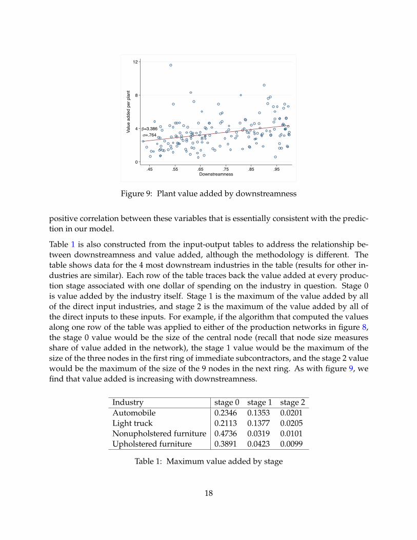
β=3.386σ=.764
0
4
8
12
Valu
e ad
ded
per p
lant
.45 .55 .65 .75 .85 .95Downstreamness
Figure 9: Plant value added by downstreamness
positive correlation between these variables that is essentially consistent with the predic-tion in our model.
Table 1 is also constructed from the input-output tables to address the relationship be-tween downstreamness and value added, although the methodology is different. Thetable shows data for the 4 most downstream industries in the table (results for other in-dustries are similar). Each row of the table traces back the value added at every produc-tion stage associated with one dollar of spending on the industry in question. Stage 0is value added by the industry itself. Stage 1 is the maximum of the value added by allof the direct input industries, and stage 2 is the maximum of the value added by all ofthe direct inputs to these inputs. For example, if the algorithm that computed the valuesalong one row of the table was applied to either of the production networks in figure 8,the stage 0 value would be the size of the central node (recall that node size measuresshare of value added in the network), the stage 1 value would be the maximum of thesize of the three nodes in the first ring of immediate subcontractors, and the stage 2 valuewould be the maximum of the size of the 9 nodes in the next ring. As with figure 9, wefind that value added is increasing with downstreamness.
Industry stage 0 stage 1 stage 2Automobile 0.2346 0.1353 0.0201Light truck 0.2113 0.1377 0.0205Nonupholstered furniture 0.4736 0.0319 0.0101Upholstered furniture 0.3891 0.0423 0.0099
Table 1: Maximum value added by stage
18
6 Conclusion
This paper proposed a mathematical formulation of Coase’s (1937) theory of the firmthat permits investigation not just of firm boundaries but also of the vertical structure ofproduction across the industry within a competitive equilibrium setting. By developinga new methodology based on recursive subdivision of tasks combined with fixed pointtheory, we proved existence of the equilibrium price function, and showed it to be unique,convex and differentiable. We showed that the optimal actions of firms given this pricefunction are unique, well-defined and continuous. We provided a consistent algorithmfor computing equilibrium prices and actions. We derived a first order condition thatcorresponds to the key marginal condition determining firm boundaries stated verballyby Coase (1937), and added an “Euler” equation relating costs of adjacent firms. We ana-lyzed the structure of production, showing that the equilibrium number of firms is finite,and that value added and the number of tasks performed in-house are increasing fromupstream to downstream. We investigated the distribution of firms, and the relationshipbetween diminishing returns to management, transaction costs and the properties of thevertical production chain. Some extensions to the model were considered, including pro-duction networks with multiple upstream partners.
There paper opens many avenues for future research. The techniques developed in thepaper are likely to have applications to other fields, such as offshoring by multinationals,or division of labor with transaction costs, failure probabilities or other frictions. In ad-dition, the model presented above was a baseline model in all dimensions, with perfectcompetition, perfect information, identical firms and identical tasks, and these assump-tions can potentially be weakened. The effect of altering contract structures could alsobe investigated, as could the various possibilities for determining upstream partners insection 4.2. On the technical side, the operator T in (3) merits further investigation. Itmay turn out to be a contraction if the metric is well chosen, or have connections to morecommon operators or optimization problems. Such analysis might further improve thealgorithms for computing prices and actions and lead to additional insights. Finally, themodel has a number of testable implications that require investigation.
7 Appendix: Computation and Remaining Proofs
7.1 Computation
To compute an approximation to the equilibrium pricing function for given δ and c, onepossibility is to take a function in P and iterate with T. However, in practice we canonly approximate the iterates, and, since T is not a contraction mapping convergence is
19
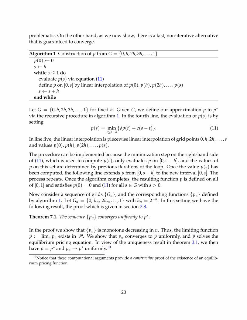
problematic. On the other hand, as we now show, there is a fast, non-iterative alternativethat is guaranteed to converge.
Algorithm 1 Construction of p from G = {0, h, 2h, 3h, . . . , 1}p(0)← 0s← hwhile s ≤ 1 do
evaluate p(s) via equation (11)define p on [0, s] by linear interpolation of p(0), p(h), p(2h), . . . , p(s)s← s + h
end while
Let G = {0, h, 2h, 3h, . . . , 1} for fixed h. Given G, we define our approximation p to p∗
via the recursive procedure in algorithm 1. In the fourth line, the evaluation of p(s) is bysetting
p(s) = mint≤s−h
{δp(t) + c(s− t)}. (11)
In line five, the linear interpolation is piecewise linear interpolation of grid points 0, h, 2h, . . . , sand values p(0), p(h), p(2h), . . . , p(s).
The procedure can be implemented because the minimization step on the right-hand sideof (11), which is used to compute p(s), only evaluates p on [0, s − h], and the values ofp on this set are determined by previous iterations of the loop. Once the value p(s) hasbeen computed, the following line extends p from [0, s− h] to the new interval [0, s]. Theprocess repeats. Once the algorithm completes, the resulting function p is defined on allof [0, 1] and satisfies p(0) = 0 and (11) for all s ∈ G with s > 0.
Now consider a sequence of grids {Gn}, and the corresponding functions {pn} definedby algorithm 1. Let Gn = {0, hn, 2hn, . . . , 1} with hn = 2−n. In this setting we have thefollowing result, the proof which is given in section 7.3.
Theorem 7.1. The sequence {pn} converges uniformly to p∗.
In the proof we show that {pn} is monotone decreasing in n. Thus, the limiting functionp := limn pn exists in P . We show that pn converges to p uniformly, and p solves theequilibrium pricing equation. In view of the uniqueness result in theorem 3.1, we thenhave p = p∗ and pn → p∗ uniformly.10
10Notice that these computational arguments provide a constructive proof of the existence of an equilib-rium pricing function.
20
7.2 Proofs from Section 3
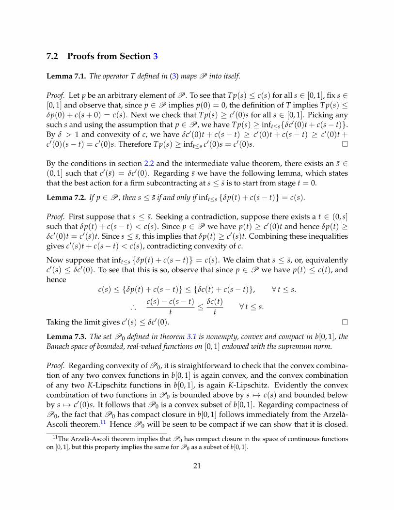
Lemma 7.1. The operator T defined in (3) maps P into itself.
Proof. Let p be an arbitrary element of P . To see that Tp(s) ≤ c(s) for all s ∈ [0, 1], fix s ∈[0, 1] and observe that, since p ∈P implies p(0) = 0, the definition of T implies Tp(s) ≤δp(0) + c(s + 0) = c(s). Next we check that Tp(s) ≥ c′(0)s for all s ∈ [0, 1]. Picking anysuch s and using the assumption that p ∈P , we have Tp(s) ≥ inft≤s{δc′(0)t + c(s− t)}.By δ > 1 and convexity of c, we have δc′(0)t + c(s − t) ≥ c′(0)t + c(s − t) ≥ c′(0)t +c′(0)(s− t) = c′(0)s. Therefore Tp(s) ≥ inft≤s c′(0)s = c′(0)s.
By the conditions in section 2.2 and the intermediate value theorem, there exists an s ∈(0, 1] such that c′(s) = δc′(0). Regarding s we have the following lemma, which statesthat the best action for a firm subcontracting at s ≤ s is to start from stage t = 0.
Lemma 7.2. If p ∈P , then s ≤ s if and only if inft≤s {δp(t) + c(s− t)} = c(s).
Proof. First suppose that s ≤ s. Seeking a contradiction, suppose there exists a t ∈ (0, s]such that δp(t) + c(s− t) < c(s). Since p ∈ P we have p(t) ≥ c′(0)t and hence δp(t) ≥δc′(0)t = c′(s)t. Since s ≤ s, this implies that δp(t) ≥ c′(s)t. Combining these inequalitiesgives c′(s)t + c(s− t) < c(s), contradicting convexity of c.
Now suppose that inft≤s {δp(t) + c(s− t)} = c(s). We claim that s ≤ s, or, equivalentlyc′(s) ≤ δc′(0). To see that this is so, observe that since p ∈ P we have p(t) ≤ c(t), andhence
c(s) ≤ {δp(t) + c(s− t)} ≤ {δc(t) + c(s− t)}, ∀ t ≤ s.
∴c(s)− c(s− t)
t≤ δc(t)
t∀ t ≤ s.
Taking the limit gives c′(s) ≤ δc′(0).
Lemma 7.3. The set P0 defined in theorem 3.1 is nonempty, convex and compact in b[0, 1], theBanach space of bounded, real-valued functions on [0, 1] endowed with the supremum norm.
Proof. Regarding convexity of P0, it is straightforward to check that the convex combina-tion of any two convex functions in b[0, 1] is again convex, and the convex combinationof any two K-Lipschitz functions in b[0, 1], is again K-Lipschitz. Evidently the convexcombination of two functions in P0 is bounded above by s 7→ c(s) and bounded belowby s 7→ c′(0)s. It follows that P0 is a convex subset of b[0, 1]. Regarding compactness ofP0, the fact that P0 has compact closure in b[0, 1] follows immediately from the Arzela-Ascoli theorem.11 Hence P0 will be seen to be compact if we can show that it is closed.
11The Arzela-Ascoli theorem implies that P0 has compact closure in the space of continuous functionson [0, 1], but this property implies the same for P0 as a subset of b[0, 1].
21
Closedness of P0 in b[0, 1] is readily apparent, since uniform limits preserve convexity,the K-Lipschitz property and the bounds defining P .
Lemma 7.4. Let p ∈P0 and define
tp(s) := arg mint≤s
{δp(t) + c(s− t)} and `p(s) := s− tp(s). (12)
Let s1 and s2 be two points with 0 < s1 ≤ s2 ≤ 1. The following statements are true:
1. Both tp(s1) and `p(s1) are well defined and single-valued.2. tp(s1) ≤ tp(s2) and tp(s2)− tp(s1) ≤ s2 − s1.3. `p(s1) ≤ `p(s2) and `p(s2)− `p(s1) ≤ s2 − s1.
Proof. Since t 7→ δp(t) + c(s1− t) is continuous and strictly convex (by convexity of p andstrict convexity of c), and since [0, s1] is compact, existence and uniqueness of tp(s1) and`p(s1) must hold.
Next we show that tp(s1) ≤ tp(s2). To simplify notation, let ti := tp(si). Suppose insteadthat t1 > t2. We aim to show that, in this case,
δp(t1) + c(s2 − t1) < δp(t2) + c(s2 − t2), (13)
which contradicts the definition of t2.12
To establish (13), observe that t1 is optimal at s1 and t2 < t1, so
δp(t1) + c(s1 − t1) < δp(t2) + c(s1 − t2).
∴ δp(t1) + c(s2 − t1) < δp(t2) + c(s1 − t2) + c(s2 − t1)− c(s1 − t1).
Given that c is strictly convex and t2 < t1, we have
c(s2 − t1)− c(s1 − t1) < c(s2 − t2)− c(s1 − t2).
Combining this with the last inequality yields (13).
Next we shown that `1 ≤ `2, where `1 := `p(s1) and `2 := `p(s2). In other words,`i = arg min`≤si
{δp(si − `) + c(`)}. The argument is similar to that for tp, but this timeusing convexity of p instead of c. To induce the contradiction, we suppose that `2 < `1.As a result, we have 0 ≤ `2 < `1 ≤ s1, and hence `2 was available when `1 was chosen.Therefore,
δp(s1 − `1) + c(`1) < δp(s1 − `2) + c(`2),
12Note that t1 < s1 ≤ s2, so t1 is available when t2 is chosen.
22
where the strict inequality is due to the fact that minimizers are unique. Rearranging andadding δp(s2 − `1) to both sides gives
δp(s2 − `1) + c(`1) < δp(s2 − `1)− δp(s1 − `1) + δp(s1 − `2) + c(`2).
Given that p is convex and `2 < `1, we have
p(s2 − `1)− p(s1 − `1) ≤ p(s2 − `2)− p(s1 − `2).
Combining this with the last inequality, we obtain
δp(s2 − `1) + c(`1) < δp(s2 − `2) + c(`2),
contradicting optimality of `2.13
To complete the proof of lemma 7.4, we also need to show that tp(s2)− tp(s1) ≤ s2 − s1,and similarly for `. Starting with the first case, we have
tp(s2)− tp(s1) = s2 − `p(s2)− s1 + `p(s1) = s2 − s1 + `p(s1)− `p(s2).
As shown above, `p(s1) ≤ `p(s2), so tp(s2)− tp(s1) ≤ s2− s1, as was to be shown. Finally,the corresponding proof for `p is obtained in the same way, by reversing the roles of tpand `p. This concludes the proof of lemma 7.4.
Lemma 7.5. Let p ∈ P0, let `p be as defined in (12), and let s be the point in (0, 1] defined inlemma 7.2. If s ≥ s, then `p(s) ≥ s. If s > 0, then `p(s) > 0.
Proof. By lemma 7.4, `p is increasing, and hence if s ≤ s ≤ 1, then `p(s) ≥ `p(s) =s− tp(s) = s. By lemma 7.2, if 0 < s ≤ s, then `p(s) = s− tp(s) = s > 0.
Lemma 7.6. If p ∈P0, then Tp is differentiable on (0, 1) with (Tp)′ = c′ ◦ `p.
Proof. Fix p ∈ P and let tp be as in (12). Fix s0 ∈ (0, 1). By Benveniste and Scheinkman(1979), to show that Tp is differentiable at s0 it suffices to exhibit an open neighbor-hood U 3 s0 and a function w : U → R such that w is convex, differentiable, satisfiesw(s0) = Tp(s0) and dominates Tp on U. To exhibit such a function, observe that in viewof lemma 7.5, we have tp(s0) < s0. Now choose an open neighborhood U of s0 such thattp(s0) < s for every s ∈ U. On U, define
w(s) := δp(tp(s0)) + c(s− tp(s0)).
Clearly w is convex and differentiable on U, and satisfies w(s0) = Tp(s0). To see thatw(s) ≥ Tp(s) when s ∈ U, observe that if s ∈ U then 0 ≤ tp(s0) ≤ s, and
Tp(s) = mint≤s{δp(t) + c(s− t)} ≤ δp(tp(s0)) + c(s− tp(s0)) = w(s).
As a result, Tp is differentiable at s0 with (Tp)′(s0) = w′(s0) = c′(`p(s0)).
13Note that 0 ≤ `1 ≤ s1 ≤ s2, so `1 is available when `2 is chosen.
23
Lemma 7.7. If p ∈P0, then Tp is strictly convex.
Proof. To see this, pick any 0 ≤ s1 < s2 ≤ 1 and any λ ∈ (0, 1). Let
ti := arg mint≤si
{δp(t) + c(si − t)} for i = 1, 2,
and t3 := λt1 + (1− λ)t2. It is easy to check that 0 ≤ t3 ≤ λs1 + (1− λ)s2, and hence
Tp(λs1 + (1− λ)s2) ≤ δp(t3) + c(λs1 + (1− λ)s2 − t3).
The right-hand side expands out to
δp[λt1 + (1− λ)t2] + c[λs1 − λt1 + (1− λ)s2 + (1− λ)t2].
Using convexity of p and strict convexity of c, we obtain
Tp(λs1 + (1− λ)s2) < λTp(s1) + (1− λ)Tp(s2).
In other words, Tp is strictly convex.
Lemma 7.8. The operator T maps P0 into itself.
Proof. Let p ∈ P0. That Tp satisfies the bounds c′(0)s ≤ p(s) ≤ c(s) was proved inlemma 7.1. That Tp is convex was shown in lemma 7.7. Finally, Tp is K-Lipschitz for K :=c′(1) because, by lemma 7.6 and convexity of c, we have (Tp)′(s) ≤ c′(`p(s)) ≤ c′(1). Thec′(1)-Lipschitz property now follows immediately from the mean value theorem.
Lemma 7.9. The operator T is continuous as a mapping from b[0, 1] to itself.
Proof. That T maps b[0, 1] into itself is trivial to prove. To see continuity of the mapping,observe that for f and g in b[0, 1] we have | inf f − inf g| ≤ sup | f − g|, and hence, for anygiven s ∈ [0, 1] and p, q ∈ b[0, 1],
| inft≤s{δp(t) + c(s− t)} − inf
t≤s{δq(t) + c(s− t)}| ≤ δ sup
t≤s|p− q| ≤ δ sup
t∈[0,1]|p− q|.
∴ |Tp(s)− Tq(s)| ≤ δ supt∈[0,1]
|p− q|.
Taking the supremum of the left hand side over s, we see that T is δ-Lipschitz as a map-ping from b[0, 1] to itself. Since every Lipschitz continuous function is continuous, weconclude that T is a continuous self mapping on b[0, 1].
24
It was shown in section 3 that an equilibrium price function exists. The proof used Tarski’sfixed point theorem. We now claim that p has a Lipschitz continuous and convex fixedpoint. The simplest way to do this is to apply a fixed point theorem to T as a mappingfrom P0 to itself. Since P0 is not a complete lattice, we use Schauder’s fixed point theo-rem instead. (Of course, this makes the earlier application of Tarski’s fixed point theoremredundant, but the proof of Tarski’s fixed point theorem is simpler, and this is the reasonwe chose to include it as well.)
Proposition 7.1. The operator T has a fixed point in P0.
Proof. In lemma 7.9 we saw that T is a continuous self mapping on b[0, 1]. Moreover, P0is a nonempty convex compact subset of b[0, 1] (lemma 7.3), and T maps P0 into itself(lemma 7.8). Schauder’s fixed point theorem now implies that T has a fixed point inP0.
Proposition 7.2. The operator T has at most one fixed point in P0.
Proof. Let p and q be two fixed points of T in P0. The proof is by induction. First we showthat there exist an k ∈ N such that p and q agree on the interval [0, 1/k]. Next we showthat if n ∈ N, n < k and p and q agree on [0, n/k], then they also agree on [0, (n + 1)/k].It follows that p and q agree on all of [0, 1].
To begin, let s be as defined in lemma 7.2. Let k be chosen such that 1/k ≤ s. Observe thatif s ≤ 1/k, then p(s) = q(s), because, in light of the definition of s, if s ≤ s, then
p(s) = mint≤s{δp(t) + c(s− t)} = c(s) = min
t≤s{δq(t) + c(s− t)} = q(s).
Turning to the induction step, let n < k and suppose that p = q on [0, n/k]. Fix s ∈[0, (n + 1)/k]. We claim that p(s) = q(s). To see this, first suppose that s ≤ s. In that casep(s) = q(s) = c(s) as shown above. Suppose instead that s > s. In that case, lemma 7.5and the definition of k yield `p(s) ≥ `p(s) = s ≥ 1/k. Therefore tp(s) = s − `p(s) ≤s− 1/k ≤ (n + 1)/k− 1/k = n/k. Exactly the same argument holds for q as well, so wehave tp(s) ≤ n/k and tq(s) ≤ n/k. This tells us that when computing the optimal actiont for either p or q, we can restrict attention to minimizing over [0, n/k]. Moreover, by theinduction hypothesis, p and q agree on [0, n/k], This leads to our conclusion:
p(s) = mint≤n/k
{δp(t) + c(s− t)} = mint≤n/k
{δq(t) + c(s− t)} = q(s).
The proof of uniqueness is complete.
Proof of theorem 3.1. Existence and uniqueness of an equilibrium price function p∗ in P0follows from propositions 7.1 and 7.2. Since p∗ ∈ P0 and the image under T of any
25
function in P0 is strictly convex (lemma 7.7), we see that Tp∗ is strictly convex. Sincep∗ = Tp∗, the function p∗ itself is strictly convex. A similar argument combined withlemma 7.6 shows that p∗ is differentiable, and (p∗)′(s) = c′(`∗(s)). Since c′ is strictly pos-itive on [0, 1], the last equality also shows that p∗ is strictly increasing. Moreover, since `∗
is Lipschitz continuous (lemma 7.4) and c is assumed to be continuously differentiable,the equation (p∗)′(s) = c′(`∗(s)) implies that p∗ is not only differentiable but also contin-uously differentiable. Finally, the claims in theorem 3.1 regarding t∗ and `∗ are immediatefrom lemma 7.4.
Proof of theorem 3.2. In view of lemma 7.2 we have `∗(s) = s and hence t∗(s) = 0 when-ever s ≤ s, so it suffices to prove that tn ≤ s for some n. This must be the case because `∗
is increasing, and hence the amount of in-house production by a firm contracting at s ≥ ssatisfies `∗(s) ≥ `∗(s) = s > 0. In other words, for firms contracting above s, each takes astep of length at least s. In particular, tn ≤ 1− ns.
Lemma 7.10. If c(x) = eθx − 1, then the equilibrium number of firms is given by (9).
Proof of lemma 7.10. Let N = N∗ be the equilibrium number of firms and let r := ln(δ)/θ.From δc′(`n+1) = c′(`n) we obtain `n+1 = `n − r, and hence `1 = `n + (n − 1)r. It iseasy to check that when c(x) = eθx − 1, the constant s in lemma 7.15 is equal to r. Hence0 < `N ≤ r. Therefore (N − 1)r < `1 ≤ Nr. From ∑N
n=1 `n = 1 and `1 = `n + (n− 1)r itcan be shown that N`1 − N(N − 1)r/2 = 1. Some straightforward algebra now yields
12
(−1 +
√1 + 8/r
)< N ≤ 1
2
(1 +√
1 + 8/r)
.
The expression for N = N∗ in (9) now follows.
Proof of proposition 3.2. This follows from the recursion p∗(tn) = δp∗(tn+1) + c(`n+1) andthe fact that p(tN) = p(0) = 0.
Proof of proposition 3.3. By theorem 3.1, the function `∗ is increasing. By construction tn ≤tn−1, and hence `n+1 = `∗(tn) ≤ `∗(tn−1) = `n. Thus part 1 holds. Part 2 follows frompart 1 and convexity of p∗.
Proof of proposition 3.1. We begin with the claim that p∗a ≤ p∗b . To construct the proof, letG = {0, h, 2h, . . . 1} be a fixed grid, and, for i = 1, 2, let pi be the approximation generatedby algorithm 1 and parameter δi. We claim that pa ≤ pb. The proof is by induction.First, observe that by (15) we have pa(h) = pb(h) = c(h). Given that the functions areconstructed by linear approximation between grid points, it follows that pa ≤ pb on [0, h].
26
Thus it remains to show that if j ∈ N and pa ≤ pb on [0, jh], then pa ≤ pb on [0, (j + 1)h].To see this, observe that if the induction hypothesis is true, then
pa((j + 1)h) = mint≤jh{δa pa(t) + c((j + 1)h− t)}
≤ mint≤jh{δb pb(t) + c((j + 1)h− t)} = pb((j + 1)h).
Thus pa ≤ pb on [0, (j + 1)h] as claimed.
Now let h = hn = 2−n, and let pa = pna and pb = pn
b . We have shown that pna ≤ pn
b . Bytheorem 7.1 we have pn
i → p∗i . Since pointwise inequalities are preserved under limits, itfollows that p∗a ≤ p∗b .
As the next step of the proof, we first show that the number of tasks carried out by themost upstream firm decreases when δ increases from δa to δb. Let `a
i be the number of taskcarried out by firm i when δ = δa, and let `b
i be defined analogously. Let N = N∗a . Seekinga contradiction, suppose that `b
N > `aN. In that case, convexity of c and (7) imply that
c′(`bN−1) = δbc′(`b
N) > δac′(`aN) = c′(`a
N−1).
Hence `bN−1 > `a
N−1. Continuing in this way, we obtain `bi > `a
i for i = 1, . . . , N. But then∑N
i=1 `bi > ∑N
i=1 `ai = 1. Contradiction.
Now we can turn to the claim that N∗b ≤ N∗a . As before, let N = N∗a , the equilibriumnumber of firms when δ = δa. If `b
N = 0, then the number of firms at δb is less thanN = N∗a and we are done. Suppose instead that `b
N > 0. In view of lemma 7.2, we haveδac′(0) ≥ c′(`a
N). Moreover, we have just shown that `aN ≥ `b
N. Combining these twoinequalities and using δb > δa, we have δbc′(0) ≥ c′(`b
N). Applying lemma 7.2 again, wesee that the N-th firm completes the good, and hence N∗b = N∗a .
7.3 Proof of Theorem 7.1
To begin the proof of theorem 7.1, suppose first that G is the fixed grid 0, h, 2h, . . . , 1, andp is the function defined in algorithm 1.
Lemma 7.11. The function p is convex on [0, 1].
Proof. Since p is piecewise linear, it suffices to show that for any consecutive s0, s1, s2 in Gwe have p(s2)− p(s1) ≥ p(s1)− p(s0). Equivalently,
p(s1) ≤12{p(s0) + p(s2)}. (14)
27
We prove this first for s0 = 0, and then proceed by induction. When s0 = 0, we haves1 = h and s2 = 2h, and (14) reduces to the claim that 2p(h) ≤ p(2h). To verify this,observe first that
p(h) = min0≤t≤0
{δp(t) + c(h− t)} = c(h), (15)
whilep(2h) = min
t≤h{δp(t) + c(2h− t)}.
On [0, h], p(t) is defined by linear interpolation between p(0) and p(h) = c(h), so inparticular p(t) = c(h)(t/h). Since c is convex, we then have
p(2h) ≥ min0≤t≤h
{c(h)(t/h) + c(2h− t)} = 2c(h) = 2p(h).
We have now confirmed that p is convex on [0, 2h]. The next step is to show that if q isconvex on [0, s1], then q is convex on [0, s2] = [0, s1 + h]. To verify this, we only need tocheck that (14) holds when q is convex on [0, s1].
To see check (14), let ti be an optimal choice corresponding to si, in the sense that ti is aminimizer of {δp(t) + c(si − t)} over 0 ≤ t ≤ si − h. Note that, by the definition of ti,
t3 :=12(t0 + t2) ≤
12(s0 − h + s2 − h) = s1 − h.
As a result, t3 was available when t1 was chosen, and we have
p(s1) ≤ δp(t3) + c(s1 − t3).
Using convexity of p on [0, s1] and the fact that t0 and t2 are both less than s1, we have
p(t3) = p(t0/2 + t2/2) ≤ p(t0) + p(t2)
2.
Using convexity of c, we have
c(s1 − t∗) = c(
s0 − t0
2+
s2 − t2
2
)≤ c(s0 − t0) + c(s2 − t2)
2.
Combining the last three inequalities, we obtain
p(s1) ≤12[{δp(t0) + c(s0 − t0)}+ {δp(t2) + c(s2 − t2)}] =
12[p(s0) + p(s2)] .
In other words, (14) is valid. Convexity is now proved.
Given s ∈ [0, 1], let t(s) is a minimizer of δp(t) + c(s − t) over [0, s − h], and let `(s) =s− t(s).
28
Lemma 7.12. Let s1 and s2 be any two points in Gn with 0 < s1 ≤ s2. The following statementsare true:
1. Both t(s1) and `(s1) are well defined and unique.
2. t(s1) ≤ t(s2) and t(s2)− t(s1) ≤ s2 − s1.
3. `(s1) ≤ `(s2) and `(s2)− `(s1) ≤ s2 − s1.
The proof is almost identical to that of lemma 7.4 and hence omitted.
Lemma 7.13. The function p is monotone increasing on [0, 1].
Proof. Since p is defined by linear interpolation, it is enough to show that p(s1) ≤ p(s2)for consecutive grid points s1 and s2 = s1 + h. The proof is by induction. Evidently theclaim is true for s1 = 0, because p(0) = 0. So now let s1 be an arbitrary point in G, andsuppose that p is monotone increasing on [0, s1]. We need to show that p(s1) ≤ p(s2). Tosee that this is the case, observe that
p(si) = δp(t(si)) + c(`(si)).
By monotonicity of t and `, we have `(s1) ≤ `(s2) and t(s1) ≤ t(s2). Moreover, c ismonotone increasing, p is monotone increasing on [0, s1], and, by definition, t(s2) ≤ s1.Putting these facts together, we obtain δp(t(s1)) + c(`(s1)) ≤ δp(t(s2)) + c(`(s2)). Hence,p(s1) ≤ p(s2), as was to be shown.
Lemma 7.14. For all s ∈ [0, 1] we have p(s) ≥ c′(0)s.
Proof. For s = 0 the result is obvious, so suppose that s > 0. Let σ ≤ min{s, h}. Using thisinequality, convexity of p and c, and the fact that p(h) = c(h), we obtain c′(0) ≤ c(h)/h =p(h)/h = p(σ)/σ ≤ p(s)/s.
Lemma 7.15. Let s ∈ G. If c′(s) ≤ δc′(0), then t(s) = 0.
Proof. Let s ∈ G with c′(s) ≤ δc′(0). The value t(s) uniquely solves min0≤t≤s−h{δp(t) +c(s− t)}. This solution is zero if c(s) < δp(t) + c(s− t) when 0 < t ≤ s− h, or, equiva-lently,
c(s)− c(s− t)t
<δp(t)
twhen 0 < t ≤ s− h.
This inequality is valid, because, by strict convexity of c, the assumption c′(s) ≤ δc′(0)and lemma 7.14,
c(s)− c(s− t)t
< c′(s) ≤ c′(0) ≤ δp(t)t
for all t with 0 < t ≤ s.
29
For the remainder of this section, we adopt the setting of theorem 7.1. In particular, weconsider a sequence of grids {Gn} Gn = {0, hn, 2hn, . . . , 1} with hn = 2−n. The corre-sponding functions are denoted by {pn}.
Lemma 7.16. The sequence {pn}∞n=1 is pointwise monotone decreasing.
Proof. Fix n ∈ N. The claim is that pn+1(s) ≤ pn(s) for all s ∈ [0, 1]. Let s1 and s2 = s1 + hnbe two consecutive points in Gn, and suppose that pn+1 ≤ pn on [0, s1]. We claim thatpn+1(s2) ≤ pn(s2) also holds. This is sufficient for pn+1(s) ≤ pn(s) on [s1, s2], given that(i) pn(s) is a linear interpolation from s1 to s2, (ii) pn+1 is a linear interpolation from s1 tos′ := (s1 + s2)/2 and then s′ to s2, and (iii) pn+1 is convex.
To show that pn+1(s2) ≤ pn(s2), recall that, by the induction hypothesis, we have pn+1 ≤pn on [0, s1]. It follows that
pn+1(s2) = mint≤s′{δpn+1(t) + c(s2 − t)}
≤ mint≤s1{δpn+1(t) + c(s2 − t)}
≤ mint≤s1{δpn(t) + c(s2 − t)}
= pn(s2),
as was to be shown.
Lemma 7.17. The sequence {qn}∞n=1 is uniformly bounded and equicontinuous.
Proof. The statement that {pn}∞n=1 is uniformly bounded means that there exists a con-
stant M independent of n with sup0≤s≤1 |pn(s)| ≤ M. This is clearly true because, onone hand, pn is nonnegative (see, e.g., lemma 7.14), and on the other hand, since {pn}is monotone decreasing (lemma 7.16) and each pn is increasing (lemma 7.13), we havepn(s) ≤ p1(1) for all s and n.
It remains to show that {pn}∞n=1 is equicontinuous. Given that pn is increasing and convex
(lemma 7.11), a sufficient condition for equicontinuity is
∃M, K ∈ N s.t.pn(1)− pn(1− hn)
hn≤ K for all n ≥ M (16)
(In other words, the slope of the function pn over the last two grid points is boundedindependent of n. Note that the bound in (16) only has to be checked for n greater thansome finite M, because finite families of continuous functions on compact sets are alwaysequicontinuous.) In what follows, we simplify notation dropping the n subscript attachedto G, p, h, t and ` (t and ` being the functions described in lemma 7.12).
30
To begin the proof, first observe that if s ∈ G, then
p(s)− p(s− h) ≤ δ{p(t(s))− p(t(s− h))}+ c′(1)h, (17)
as follows the fact that, by lemma 7.12 and convexity of c,
c(`(s))− c(`(s− h)) ≤ c′(1){`(s)− `(s− h)} ≤ c′(1){s− (s− h)} = c′(1)h
It is also the case that if s ∈ G and σ(s) := inf{r ∈ G : r ≥ t(s)}, then
p(t(s))− p(t(s− h)) ≤ p(σ(s))− p(σ(s)− h) (18)
This inequality follows from lemma 7.12, which tells us that t(s)− t(s− h) ≤ s− (s− h) =h, or t(s − h) ≥ t(s) − h. Hence, applying monotonicity and convexity of p, we havep(t(s)) − p(t(s − h)) ≤ p(t(s)) − p(t(s) − h) ≤ p(σ(s)) − p(σ(s) − h), which is (18).Combining (17) and (18), we obtain the recursion
p(s)− p(s− h) ≤ δ{q(σ(s))− q(σ(s)− h)}+ c′(1)h. (19)
In particular, if we define sj := σj(1) = σ ◦ σ ◦ · · · ◦ σ(1), then, from (19),
p(sj)− p(sj − h) ≤ δ{p(sj+1)− p(sj+1 − h)}+ c′(1)h. (20)
Now let s be the s ∈ (0, 1] that satisfies c′(s) = δc′(0). The significance of s is that, in viewof lemma 7.15, we have `(s) = s, and t(s) = 0. Moreover, since ` is increasing, if sj ≥ s,then `(sj) ≥ s. As a consequence, provided that sj ≥ s, we have
sj+1 ≤ t(sj) + h = sj − `(sj) + h ≤ sj − s + h.
Starting at s0 = 1 and iterating on this inequality, we obtain
sj ≤ 1− j(s− h) (21)
Recall that h = hn in fact depends on n, but s does not (see lemma 7.15). It followsthat there exists an M ∈ N such that s − hM > 0. Applying (21), we can then take Jindependent of n with sJ = 0. Iterating backwards on (20) starting at s0 = 1, we have
p(1)− p(1− h) ≤ δJ{p(sJ)− p(sJ − h)}+ c′(1)hJ
∑i=1
δi = c′(1)hJ
∑i=1
δi.
Dividing through by h gives (16), and equicontinuity is established.
Since {pn}∞n=1 is monotonically decreasing and bounded below by zero, the function p :=
limn→∞ pn is well-defined.
31
Lemma 7.18. The function p is continuous, and {pn}∞n=1 converges to p uniformly.
Proof. Lemma 7.17 and the Arzela -Ascoli theorem imply that {pn}∞n=1 has a uniformly
convergent subsequence. Since {pn}∞n=1 is monotone decreasing and converges pointwise
to p, the entire sequence converges uniformly to p. Since continuity is preserved underuniform limits, the function p is continuous.
Theorem 7.2. The function p is a solution to the equilibrium price equation (2).
Proof. Evidently p(0) = 0. In view of lemma 7.14, p is not the zero function (i.e., non-trivial). It remains only to show that (2) holds. Since both p and c are continuous, theleft-hand side and right-hand side of (2) are both continuous in s (the right-hand side bythe theorem of the maximum). Since continuous functions that agree on a dense subset of(0, 1] must agree everywhere on (0, 1] it suffices to show that (2) holds for all s > 0 in thedyadic rationals ∪nGn. We now fix such s ∈ ∪nGn and show that (2) holds.
Since s ∈ ∪nGn, there exists an N1 ∈ N such that s ∈ Gn whenever n ≥ N1. For such n wehave s ∈ Gn and s > 0, implying that (11) holds. In particular,
pn(s) = mint≤s−hn
{δpn(t) + c(s− t)},
and hencep(s) = lim
n→∞pn(s) = lim
n→∞min
t≤s−hn{δpn(t) + c(s− t)}.
It is therefore sufficient for the theorem to establish that this expression agrees with theright-hand side of (2). In other words, we aim to show that
limn→∞
mint≤s−hn
{δpn(t) + c(s− t)} = mint≤s{δ p(t) + c(s− t)}. (22)
Here the left-hand side is the limit of pn(s), which is monotonically decreasing. Regardingthe right-hand side, we write g(t) = δ p(t) + c(s− t). Fixing ε > 0, the problem is then toshow that
∃N ∈ N s.t. n ≥ N =⇒ mint≤s−hn
{δpn(t) + c(s− t)} < mint≤s
g(t) + ε. (23)
Since pn → p uniformly, we choose N2 ∈ N such that n ≥ N2 implies supx(pn(x) −p(x)) < ε/2. For such n, we have
mint≤s−hn
{δpn(t) + c(s− t)} ≤ mint≤s−hn
{δp(t) + ε/2 + c(s− t)}.
To summarize,
n ≥ max{N1, N2} =⇒ mint≤s−hn
{δpn(t) + c(s− t)} ≤ mint≤s−hn
g(t) + ε/2.
32
Since g is continuous on [0, s] and hn ↓ 0, we can choose an N3 such that
n ≥ N3 =⇒ mint≤s−hn
g(t) ≤ mint≤s
g(t) + ε/2.
Combining these last two inequalities, we have established that (23) holds when N :=max{N1, N2, N3}.
References
[1] Acemoglu, Daron, Simon Johnson, Todd Mitton, “Determinants of Vertical Integration: Fi-nancial Development and Contracting Costs,” The Journal of Finance 64:3 (2009), 251–1290.
[2] Acemoglu, Daron, Philippe Aghion, Rachel Griffith, and Fabrizio Zilibotti, “Vertical Integra-tion and Technology: Theory and Evidence,” Journal of the European Economic Association 8:5(2010), 989–1033.
[3] Aghion, Philippe, and Richard Holden, “Incomplete Contracts and the Theory of the Firm:What Have We Learned in the Past 25 Years,” Journal of Economic Perspectives 25:2 (2011),181–197.
[4] Antras, Pol, Davin Chor, “Organizing the Global Value Chain,” mimeo (2011).
[5] Antras, Pol, Davin Chor, Thibault Fally, and Russell Hillberry, “Measuring the Upstream-ness of Production and Trade Flows,” American Economic Review Papers and Proceedings 102:3(2012), 412–416.
[6] Arrow, Kenneth J., “The Organization of Economic Activity: Issues Pertinent to the Choiceof Market versus Non-market Allocations” (pp. 47–64) in Analysis and Evaluation of PublicExpenditures: The PPP System, Volume 1 (Washington, DC: Government Printing Office, 1969)
[7] Arrow, Kenneth J., The Limits of Organization (New York, NY: Norton, 1974).
[8] Arrow, Kenneth J., “Vertical Integration and Communication,” Bell Journal of Economics 6:1(1975), 173–83.
[9] Becker, Gary S., and Kevin M. Murphy, “The Division of Labor, Coordination Costs, andKnowledge,” Quarterly Journal of Economics 107:4 (1992), 1137–1160.
[10] Benveniste, Lawrence M., and Jose A. Scheinkman, “On the Differentiabilityof the ValueFunction in Dynamic Models of Economics,” Econometrica 47:3 (1979) 727–32.
[11] Blau, Peter M., and Marshall W. Meyer, Bureaucracy in Modern Society (New York, NY: Ran-dom House, 1987).
33
[12] Bolton, Patrick, and Mathias Dewatripont, “The Firm as a Communication Network,” Quar-terly Journal of Economics 109:4 (1994) 809–839.
[13] Bresnahan, Timothy F., and Jonathan D. Levin, “Vertical Integration and Market Structure,”NBER working paper no. 17889 (2012).
[14] Chandler, Alfred D., The Visible Hand: The Managerial Revolution in American Business (Har-vard University Press, 1977)
[15] Coase, Ronald H., “The Nature of the Firm,” Economica 4:16 (1937), 386–405.
[16] Costinot, Arnaud, “On the Origins of Comparative Advantage,” Journal of International Eco-nomics 77:2 (2009), 255–264.
[17] Costinot, Arnaud, Jonathan Vogel, and Su Wang, “An Elementary Theory of Global SupplyChains,” NBER working paper no. 16936 (2011).
[18] Demsetz, Harold, “Theory of the Firm Revisisted,” Journal of Law and Economics 4:1 (1988),141–162.
[19] Fally, Thibault, “On the Fragmentation of Production in the U.S.,” mimeo (2012).
[20] Gabre-Madhin, Eleni Z., “Market Institutions,Transaction Costs, and Social Capital in theEthiopian Grain Market,” International Food Policy Research Institute Research Report 124.
[21] Garicano, Luis, “Hierarchies and the Organization of Knowledge in Production,” Journal ofPolitical Economy 108:5 (2000), 874–904.
[22] Garicano, Luis, and Esteban Rossi-Hansberg, “Organization and Inequality in a KnowledgeEconomy,” Quarterly Journal of Economics 121:4 (2006), 1383–1435.
[23] Geanakoplos, John, and Paul Milgrom, “A Theory of Hierarchies Based on Limited Manage-rial Attention,” Journal of the Japanese and International Economies 5:3 (1991), 205–225.
[24] Grossman, Gene, and Elhanan Helpman, “Integration versus Outsourcing in Industry Equi-librium,” Quarterly Journal of Economics 117:1 (2002), 85–120
[25] Grossman, Gene, and Esteban Rossi-Hansberg, “Trading Tasks: A Simple Theory of Off-shoring,” American Economic Review 98:5 (2008), 1978–1997.
[26] Grossman, Gene, and Esteban Rossi-Hansberg, “Task Trade between Similar Countries,”Econometrica 80:2 (2012), 593–629.
[27] Grossman, Sandford, and Oliver Hart, “The Costs and Benefits of Ownership: A Theory ofVertical and Lateral Integration,” Journal of Political Economy 94:4 (1986), 691–719.
[28] Hart, Oliver, and Bengt Holmstrom, “A Theory of Firm Scope,” Quarterly Journal of Economics125:2 (2010), 483–513.
34
[29] Hart, Oliver, and John Moore, “Property Rights and the Nature of the Firm,” Journal of Polit-ical Economy 98:6 (1990), 1119–1158.
[30] Hayek, Friedrich A., “The Use of Knowledge in Society,” American Economic Review 35:4(1945), 519–530.
[31] Holmstrom, Bengt, and Paul Milgrom, “The Firm as an Incentive System,” American Eco-nomic Review 84:4 (1994), 972–991.
[32] Houthakker, Hendrik S., “Economics and Biology: Specialization and Speciation,” Kyklos 9,181–189.
[33] Jensen, Michael C., and William H. Meckling, “Theory of the Firm: Managerial Behavior,Agency Costs and Ownership Structure,” Journal of Financial Economics 3:4 (1976), 305–360.
[34] Klein, Benjamin, Robert Crawford, and Armen Alchian, “Vertical Integration, AppropriableRents, and the Competitive Contracting Process,” Journal of Law and Economics 21:2 (1978),297–326.
[35] Lucas, E. Robert, “On the Size Distribution of Business Firms,” Bell Journal of Economics 9:2(1978), 508-523.
[36] McAfee, Preston and John McMillan, “Organizational Diseconomies of Scale,” Journal of Eco-nomics and Management Strategy 4:3 (1995), 399–426.
[37] North, Douglass C., “Institutions, Transaction Costs and Productivity in the Long Run,”Washington University in St. Louis, Economics working paper archive no. 9309004 (1993).
[38] Polanec, Saso, “On the Evolution of Size and Productivity in Transition: Evidence fromSlovenian Manufacturing Firms,” KU Leuven LICOS Centre for Transition Economics, Dis-cussion Paper 154/2004(2004).
[39] Rasmusen, Eric B., and Todd Zenger, “Diseconomies of Scale in Employment Contracts,”Journal of Law, Economics and Organization 6:1 (1990), 65–92.
[40] Robertson, Dennis H., Control of Industry (London: Nisbet and Co., 1923).
[41] Sandefur, Justin, “On the Evolution of the Firm Size Distribution in an African Economy,”The Centre for the Study of African Economies, Oxford University, Working Paper 2010-05(2010).
[42] Seabright, Paul, The Company of Strangers: a Natural History of Economic Life (Princeton, NJ:Priceton University Press, 2010)
[43] Simon, Robert A., Administrative Behavior, a Study of Decision Making Processes in Administra-tive Organization (New York, NY: The Macmillan Co., 1947)
[44] Smith, Adam, The Wealth of Nations (1776, reprinted by University of Chicago Press in 1976)
35
[45] Tsuji, Masasugu, “Automotive Clusters in Japan: The Aichi Region,” mimeo, OSIPP, OsakaUniversity (2004).
[46] Williamson, Oliver E., “Transaction-Cost Economics: The Governance of Contractual Rela-tions,” Journal of Law and Economics 22:2 (1979), 233–261.
[47] Williamson, Oliver E., “The Economics of Organization: The Transaction Cost Approach,”American Journal of Sociology 87:3 (1981), 548–577.
[48] Williamson, Oliver E., Markets and Hierarchies: Analysis and Antitrust Implications (New York,NY: Free Press, 1975).
[49] Yang, Xiaokai and Yew-Kwang Ng, Specialization and Economic Organization (Amsterdam:North-Holland, 1993).
36