Embed Size (px)
Citation preview
Coarse-scale constrained ensemble
Kalman filter for subsurface characterization
S. Akella ∗,a , A. Datta-Gupta b , Y. Efendiev c
aDept. of Earth & Planetary Sciences and Dept. of Applied Mathematics &Statistics, The Johns Hopkins University, Baltimore, MD 21218, USA
bDepartment of Petroleum Engineering, Texas A&M University, College Station,TX 77843, USA
cDepartment of Mathematics, Texas A&M University, College Station, TX 77843,USA
Abstract
In this paper we propose a way to integrate data at different spatial scales usingthe ensemble Kalman filter (EnKF), such that the finest scale data is sequentiallyestimated, subject to the available data at the coarse scale(s), as an additionalconstraint. Relationship between various scales has been modeled via upscalingtechniques. The proposed coarse-scale EnKF algorithm is recursive and easily imple-mentable. Our numerical results with static as well as dynamic, coarse-scale dataprovide improved fine-scale field estimates when compared to the results with reg-ular EnKF (which did not incorporate the coarse-scale data). We also tested ouralgorithm with various precisions of the coarse-scale data to account for the inexactrelationship between the fine and coarse scale data. As expected, the results showthat higher precision in the coarse-scale data, yielded improved estimates.
Key words:Ensemble Kalman filter, Multiscale data, Upscaling models, Sequential dataassimilation
∗ Correspoding author. Address: Dept. of Earth & Planetary Sciences and Dept.of Applied Mathematics & Statistics, The Johns Hopkins University, Baltimore,MD 21218, USAEmail address: [email protected] (S. Akella)
1 Introduction
The principal objective of data assimilation methods [28] is to combine theinformation provided by measured data and a (numerical) forecast model toobtain an improved estimate of the system state (and parameters). Unlike vari-ational methods which require availability of complex adjoint models for dataassimilation, the ensemble Kalman filter (EnKF) can be quickly implementedand one can also obtain uncertainty estimates via error variance-covariancepropagation; see [21] and references therein for further details. The EnKF isa sequential Monte Carlo method based on Bayes theorem. The method isincreasingly being used for estimating unknown model state and parametersin various geological and hydrological models [31,5,29].
Broadly speaking, the measured data used for description of reservoir porosityand permeability characterization consist of static and dynamic data. Staticdata such as well logs, core samples can resolve heterogeneity at a scale ofa few inches or feet with high reliability. However, dynamic data such asfractional flow (defined as the ratio of the injection fluid to the total fluidproduced at the production wells; or water cut), pressure transient and tracertest data typically scan the length scales comparable to the inter-well dis-tances. Additional dynamic data such as time-lapse seismic images [30] canprovide improved spatial sampling, but at a lower precision. A majority ofprevious studies on uncertainty quantification in reservoir performance fore-casting using EnKF have mostly dealt with integration of dynamic data (fore.g., [32,35,24]). However it is widely recognized that integration of additionalmultiscale data could further reduce the uncertainty (see [27,14,15] and ref-erences therein). We also note that when compared to fine-scale simulations,coarse-scale simulations are many folds computationally efficient (for e.g., seeintroduction in [36]). With that perspective, integration of data at coarse-andfine-scales, is an important objective. We would like to emphasize that to thebest of our knowledge, integration of multiscale data using EnKF to estimatefine-scale fields for subsurface characterization has not yet been addressed.Also, our method could be generalized to other sequential data assimilationmethods such as particle filtering (where, rather than updating the ensemblemembers model state, we update the probability assigned to each ensemblemember based on model data misfit). The main reason why we used EnKF inthis paper is because it requires fewer ensemble members than the particlefilters, see [29] and references therein for further details.
In this paper, apart from the water cut data, we consider two kinds of coarse-scale measured data as well. The coarse-scale data are assumed to be perme-ability and/or saturation at some specified level of precision. The unknownvariables: permeability, at the fine-scale, are estimated using a modificationto the EnKF algorithm, linking the data at different scales via upscaling. It
2
is important to resolve fine-scale heterogeneity for various purposes such as,enhanced oil recovery, environmental remediation, etc. The main idea behindupscaling is to obtain an effective coarse-scale permeability which yields thesame average response as that of the underlying fine-scale field, locally. Singlephase flow upscaling procedures for two phase flow problem have been dis-cussed by many authors; see e.g., [6,3,11] and also Section 3.1. We will refer toour proposed variant of EnKF as coarse-scale EnKF. Assimilation using dynamicdata, such as fractional flow data only, is therefore referred to as regular EnKF.First we consider coarse-scale permeability data, which can be obtained eitherfrom geologic consideration or coarse-scale inversion of dynamic, fractionalflow data on a coarse grid as considered in [27,15]. We note that coarse-scaleinversion of the dynamic data usually uses more accurate and reliable priormodels and, thus, the inversion results have higher precision. In Section 5 weillustrate a procedure for such a coarse-scale inversion. This coarse-scale, staticdata can be viewed as a constraint, which is to be satisfied up to the prescribedvariance for obtaining the fine-scale estimates in every data assimilation cy-cle. Upscaling methods relate the solution at the fine-scale to the coarse-scale,therefore in the Kalman filter context, it amounts to modeling a nonlinearobservation operator. In our coarse-scale EnKF approach, we use the measureddata in batches, such that the estimate with one data becomes a prior whileassimilating the other observation (see Section 3 for further details). Thoughin this paper we used coarse-scale data at only one scale, our approach canbe easily generalized to assimilate data at multiple scales by appropriatelymodeling the linkage between different scales.
The second kind of coarse-scale observed data we consider is dynamic, andis motivated based on the increasing availability of time-lapse seismic images(or 4d seismic data). Integration of inverted 4d seismic data (at fine-scale)using the EnKF has been addressed in [9] and [34]. In this article, we considerthe seismic data, not to correspond to the finest scale, but to a coarse-scale,since time-lapse seismic data typically will have a lower resolution comparedto the fine-scale geologic model [22]. As the time-lapse seismic data is collectedonly at specific time intervals, we used coarse-scale fluid saturation, as mea-sured data to be available at a prescribed level of precision (which accountsfor the inaccuracies involved in inversion of 4d seismic data) and only for cer-tain assimilation cycles. Therefore unlike the coarse-scale static permeabilitydata considered earlier, the coarse-scale saturation data is assimilated only incertain assimilation cycles (see Section 4.3 for details).
For the purpose of self-contendness and notational clarity, we briefly review thegoverning equations, sequential data assimilation using the ensemble Kalmanfilter in Section 2, which is followed by a description of the coarse-scale EnKF al-gorithm (Section 3). For our numerical results (Section 4), we consider a five-spot pattern, with the injection well placed in the middle of a rectangulardomain and four production wells located at the vertices of the rectangle.
3
A reference case is used to provide true data, which is randomly perturbedto obtain synthetic measurements. A comparison of the regular EnKF withthe coarse-scale EnKF (Sections 4.1 and 4.2 respectively) shows that usingcoarse-scale permeability data (via coarse-scale EnKF) significantly improvesthe fine-scale estimates as well as future fractional flow prediction. We ob-tained similar improvements with coarse-scale saturation data (Section 4.3).But due to the fact that it was assimilated infrequently, the fine-scale estimatesand prediction is not as good as using coarse-scale permeability, neverthelessbetter than those obtained using regular EnKF. In Section 5, we demonstratethat the coarse-scale permeability data can be obtained in the absence of anyprior geologically derived or coarse-scale inverted permeability data. To ac-complish this, we first develop a model which maps fine-scale to coarse-scalewater cuts. Thereafter, the mapped coarse-scale water cut is used to estimatethe coarse-scale permeability field.
2 Preliminaries
2.1 Fine-scale model
In this paper, we consider two-phase flow in a subsurface formation under theassumption that the displacement is dominated by viscous effects. For simplic-ity, we neglect the effects of gravity, compressibility, and capillary pressure,although our proposed approach is independent of the choice of physical mech-anisms. Also, porosity will be considered to be constant. The two phases willbe referred to as water and oil (or a non-aqueous phase liquid), designatedby subscripts w and o, respectively. We write Darcy’s law for each phase asfollows:
vj = −krj(S)
µj
κf∇pr, (1)
∇ · (λ(S)κf∇pr) = h, , (2)
λ(S) =krw(S)
µw
+kro(S)
µo
, f(S) =krw(S)/µw
krw(S)/µw + kro(S)/µo
,
v = vw + vo = −λ(S)κf · ∇pr, (3a)
φ∂S
∂t+ v · ∇S = 0. (3b)
The above descriptions are referred to as the fine-scale model of the two-phaseflow problem. Here κf is the (fine-scale) permeability of the medium, λ(S) isthe total mobility, µj denotes phase viscosity, pr is the pressure, h is thesource term, φ and S denote porosity and water saturation (volume fraction),respectively.
4
2.2 Sequential estimation using EnKF
Using dynamic measured data such as water cut, we can sequentially estimatethe unknown parameters (permeability, porosity, etc.) and state variables suchas pressure, water saturation (two-phase flow) and production data at welllocations using the EnKF as discussed in [32,23,24,8,2,21]. Following these pre-vious works, in this paper we assume that the only dynamic data available iswater cut data, and that porosity is known. The combined state-parameterto be estimated are given by Ψ = [ln(κf ),pr,S,Wc]
T . Where ln(·) is naturallogarithm of permeability field and Wc denotes water cut; in order to distin-guish observed water cut from model predicted water cut, now onwards wewill denote the observed water cut data Wo
c, by y.
The EnKF introduced by Evensen, 1994 [20] is a sequential Monte Carlo methodwhere an ensemble of model states evolve in state-space with mean as the bestestimate and spread of the ensemble as the error covariance, as summarized inthe following steps. Each of the ensemble members is forecasted independently(in this work, we neglected modeling errors),
Ψ(i)n+1 = F [Ψ(i)
n ], (4)
where F [·] is the forecast operator (eqns. 1–3b), superscript (i) denotes the ith
ensemble member; now onwards we will drop the time subscript. The ensemblemean and covariance are defined as,
Ψ =1
Ne
Ne∑i=1
Ψ(i), (5a)
Pf ≈ 1
Ne − 1A′ (A′)T , (5b)
where A′ = (b(1),b(2), . . . ,b(Ne)), b(i) = Ψ(i) −Ψ, and Ne is the number ofensemble members. The observation vector for each ensemble member is givenby,
y(i) = H[Ψt] + ν(i), (6)
where H[Ψt] is the observed data from the truth and ν(i) represents observa-tional errors, which are i.i.d. samples [4] from a normal distribution with zeromean and variance, R. We note that if only the water cut data is being mea-sured, the mapping from model-to-observational space, H is trivially equal to[0 0 0 I] , since Ψ = [ln(κ), pr, S, Wc]
T .
The forecasted ensemble (eqn. 4) is updated by assimilating the observed data,
Ψ(i) = Ψ(i) + K(y(i) −H[Ψ(i)]), (7)
5
where K is the Kalman gain, given by
K = PfHT [HPfHT + R]−1.
Computationally efficient implementation of the EnKF is discussed for e.g.,in [21,5]. We use the above set of corrected ensemble states, Ψ(i)Ne
i=1 in thesimulation model (eqn. 4) to predict until the next set of observational datais available.
3 Coarse-scale constrained EnKF
The EnKF presented so far, used only the dynamic, production data (watercut) y, with error ν = y − H[Ψt], ν ∼ N (0,R) to update the ensemble(eqn. 7). In addition to y, if we are also given static data (as mentioned inthe Introduction), which is another set of independently measured data, z.Assuming that the corresponding measurement error is given by ω = z −U[Ψt], ω ∼ N (0,Q); U : Ψ 7→ z. Its likelihood is given by
p(z|Ψ) ∝ exp−1
2(z−U[Ψ])T Q−1 (z−U[Ψ])︸ ︷︷ ︸
Jz
. (8)
If this static data z, corresponds to coarse-scale permeability data [15,27],then U = [U 0 0 0]. Where U : κf 7→ κc, is a nonlinear mapping that mapsthe fine-scale permeability field (κf ) to coarse-scale field (κc) via an upscalingprocedure (e.g., [10,11]), details are provided in Section 3.1.
Now, our goal is to obtain an estimate which is based on both of the abovedynamic and static data. The likelihood of y is given by
p(y|Ψ) ∝ exp−1
2(y−H[Ψ])T R−1 (y−H[Ψ])︸ ︷︷ ︸
Jy
.
The probability distribution function (pdf) of the predicted ensemble,
p(Ψ) ∝ exp−1
2(Ψ−Ψ)T (Pf )−1 (Ψ−Ψ︸ ︷︷ ︸
Jf
),
where Ψ and Pf are the predicted ensemble mean and covariance respectively(eqns. 5a–5b). Then, using Bayes theorem, we obtain
p(Ψ|z,y) =p(Ψ, z,y)
p(z,y)=p(z,y|Ψ) p(Ψ)
p(z,y)∝ p(z,y|Ψ)p(Ψ) = p(z|Ψ) p(y|Ψ) p(Ψ).︸ ︷︷ ︸
∝ p(Ψ|y)
6
The last term in above equation implies that the two independent data, y andz can be sequentially assimilated in the following two steps. We first assimilateobservation y to obtain an intermediate ensemble, Ψ(i)Ne
i=1, as discussed inSection 2.2.
p(Ψ) = p(Ψ|y) ∝ exp−(Jf + Jy), (9)
This intermediate ensemble and likelihood in eqn. (8), can then be combinedto obtain the final estimate Ψ(i)Ne
i=1.
p(Ψ) = p(Ψ|z,y) ∝ exp−(Jf + Jy + Jz). (10)
Therefore, in a least-squared sense, the final estimate maximizes the poste-rior pdf p(Ψ|z,y), which corresponds to the minimum of J = Jz + Jy + Jf .
See Appendix A for further details (where we show that the solution Ψ(i)
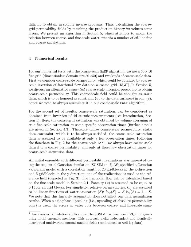
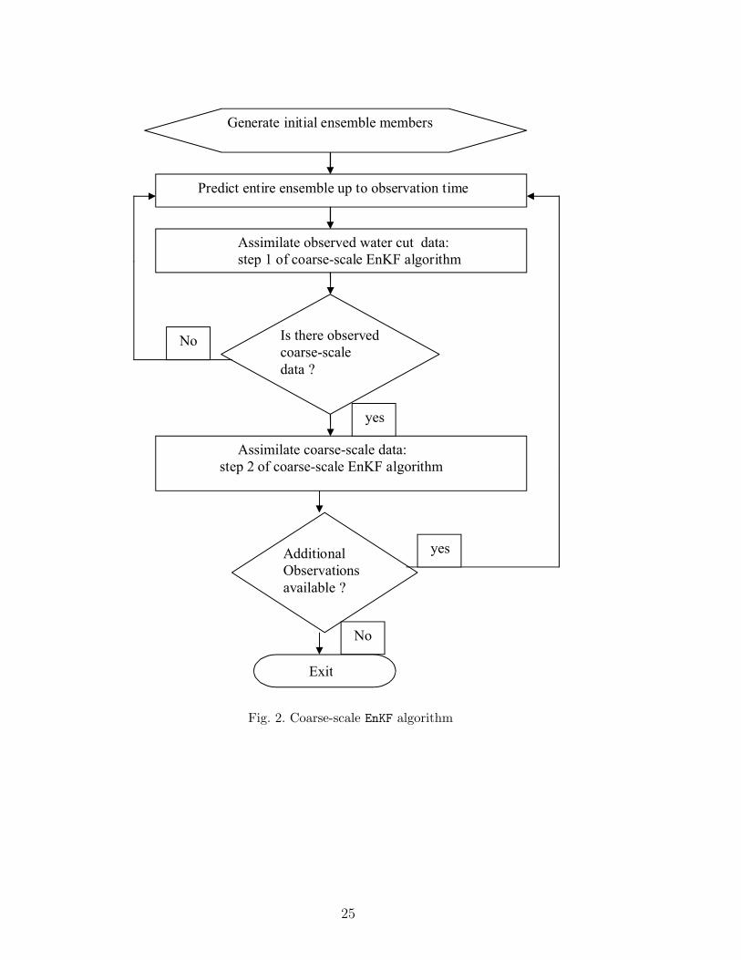
corresponds to the minimum of J , for any ith ensemble member). The coarse-scale EnKF algorithm is detailed in Appendix B, and a flow chart is givenin Fig. 2.
3.1 Upscaling methods
In brief, the main idea behind upscaling of absolute fine-scale permeability isto obtain effective coarse-scale permeability for each coarse-grid block. Oncethe upscaled absolute permeability is computed, the original equations aresolved on the coarse-grid, without changing the form of relative permeabilitycurves. This is an inexpensive calculation, since the pressure update involvesonly solving the pressure equation on the coarse-grid, and one can take largertime step for solving the transport equation. In our numerical simulations,the fine-grid is coarsened 10 times in each direction. These kinds of upscalingtechniques in conjunction with the upscaling of absolute permeability havebeen used in groundwater applications (see e.g., [13,12,11]).
The link between the coarse and the fine-scale permeability fields is usuallynontrivial because one needs to take into account the effects of all the scalespresent at the fine level. In the past simple arithmetic, harmonic or poweraverages have been used to link properties at various scales. These averagescan be reasonable for low heterogeneities or for volumetric properties suchas porosity. For permeabilities, simple averaging can lead to inaccurate andmisleading results. In this paper we use the flow-based upscaling methodsusing local solutions of the equations [10,36].
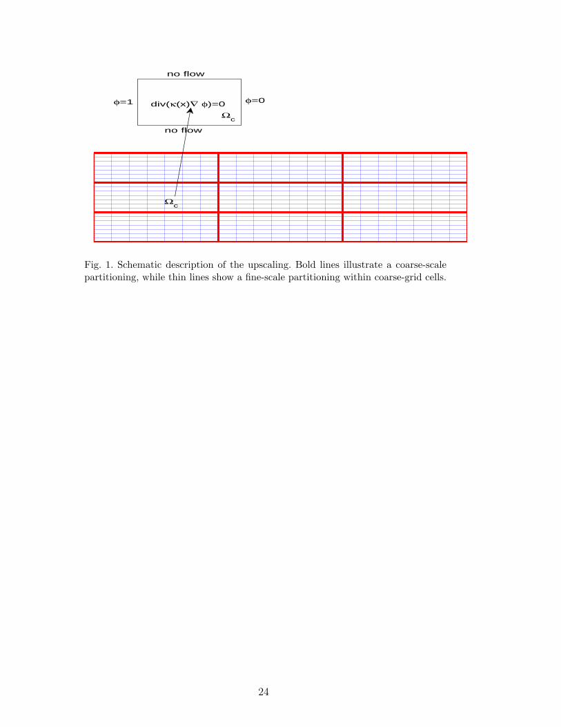
First, we briefly describe flow based upscaling methods. Consider the fine-scalepermeability that is defined in the domain with underlying fine grid as shownin Figure 1. On the same graph we illustrate a coarse-scale partition of thedomain. To calculate the coarse-scale permeability field at this level we needto determine it for each coarse block, Ωc. The coarse block permeability can
7
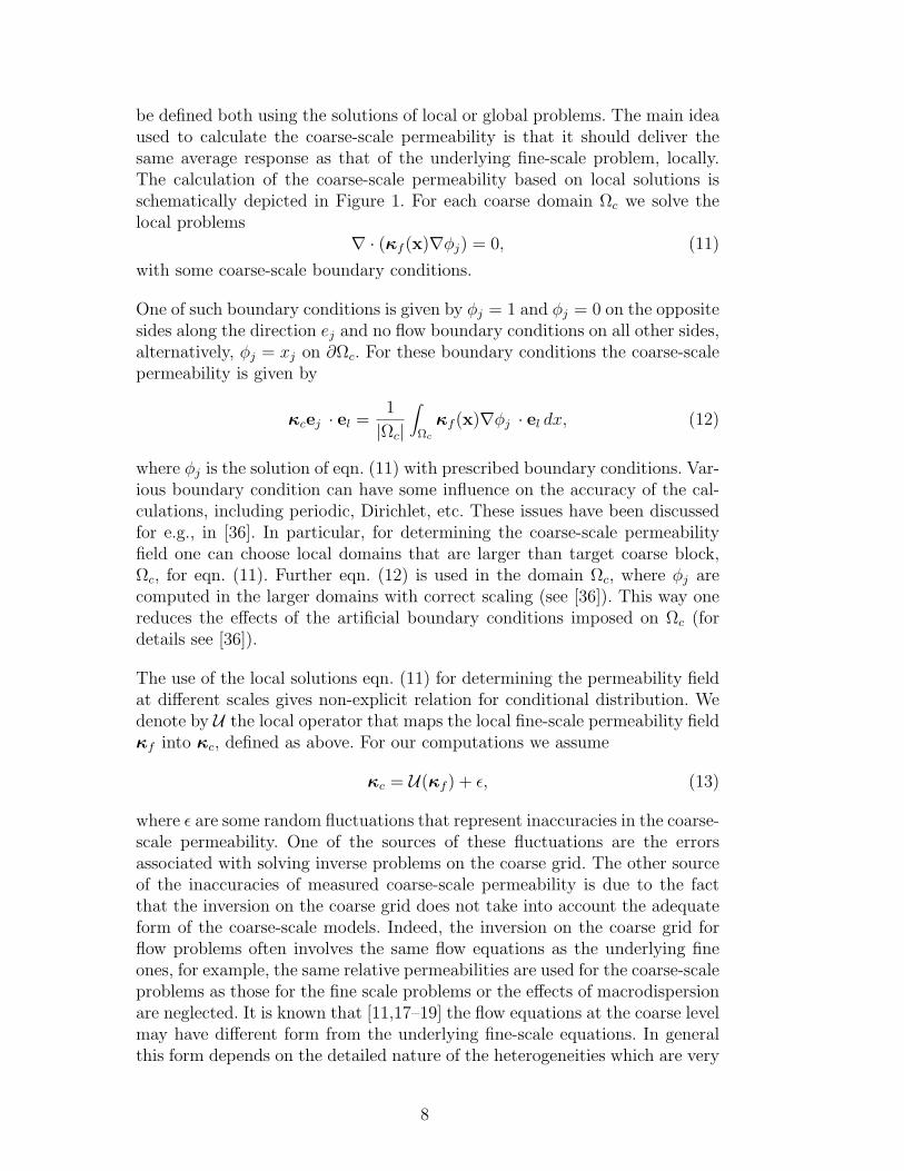
be defined both using the solutions of local or global problems. The main ideaused to calculate the coarse-scale permeability is that it should deliver thesame average response as that of the underlying fine-scale problem, locally.The calculation of the coarse-scale permeability based on local solutions isschematically depicted in Figure 1. For each coarse domain Ωc we solve thelocal problems
∇ · (κf (x)∇φj) = 0, (11)
with some coarse-scale boundary conditions.
One of such boundary conditions is given by φj = 1 and φj = 0 on the oppositesides along the direction ej and no flow boundary conditions on all other sides,alternatively, φj = xj on ∂Ωc. For these boundary conditions the coarse-scalepermeability is given by
κcej · el =1
|Ωc|
∫Ωc
κf (x)∇φj · el dx, (12)
where φj is the solution of eqn. (11) with prescribed boundary conditions. Var-ious boundary condition can have some influence on the accuracy of the cal-culations, including periodic, Dirichlet, etc. These issues have been discussedfor e.g., in [36]. In particular, for determining the coarse-scale permeabilityfield one can choose local domains that are larger than target coarse block,Ωc, for eqn. (11). Further eqn. (12) is used in the domain Ωc, where φj arecomputed in the larger domains with correct scaling (see [36]). This way onereduces the effects of the artificial boundary conditions imposed on Ωc (fordetails see [36]).
The use of the local solutions eqn. (11) for determining the permeability fieldat different scales gives non-explicit relation for conditional distribution. Wedenote by U the local operator that maps the local fine-scale permeability fieldκf into κc, defined as above. For our computations we assume
κc = U(κf ) + ε, (13)
where ε are some random fluctuations that represent inaccuracies in the coarse-scale permeability. One of the sources of these fluctuations are the errorsassociated with solving inverse problems on the coarse grid. The other sourceof the inaccuracies of measured coarse-scale permeability is due to the factthat the inversion on the coarse grid does not take into account the adequateform of the coarse-scale models. Indeed, the inversion on the coarse grid forflow problems often involves the same flow equations as the underlying fineones, for example, the same relative permeabilities are used for the coarse-scaleproblems as those for the fine scale problems or the effects of macrodispersionare neglected. It is known that [11,17–19] the flow equations at the coarse levelmay have different form from the underlying fine-scale equations. In generalthis form depends on the detailed nature of the heterogeneities which are very
8
difficult to obtain in solving inverse problems. Thus, calculating the coarse-grid permeability fields by matching the production history introduces someerrors. We present an algorithm in Section 5, which attempts to model therelation between coarse- and fine-scale water cuts via a number of off-line fineand coarse simulations.
4 Numerical results
For our numerical tests with the coarse-scale EnKF algorithm, we use a 50×50fine grid (dimensionless domain size 50×50) and two kinds of coarse-scale data.First we consider coarse-scale permeability, which could be obtained by coarse-scale inversion of fractional flow data on a coarse grid [15,37]. In Section 5,we discuss an alternative sequential coarse-scale inversion procedure to obtaincoarse-scale permeability. This coarse-scale field could be thought as staticdata, which is to be honored as constraint (up to the data variance) in eqn. (8),hence we need to always assimilate it in our coarse-scale EnKF algorithm.
For the second set of results, coarse-scale saturation, can be considered asobtained from inversion of 4d seismic measurements (see Introduction, Sec-tion 1). Here, the coarse-grid saturation was obtained by volume averaging oftrue fine-scale saturation at some specific observation times (further detailsare given in Section 4.3). Therefore unlike coarse-scale permeability, staticdata constraint, which is to be always satisfied, the coarse-scale saturationdata is assumed to be available at only a few observation times. Followingthe flowchart in Fig. 2 for the coarse-scale EnKF, we always have coarse-scaledata if it is coarse permeability; and only at those few observation times forcoarse-scale saturation data.
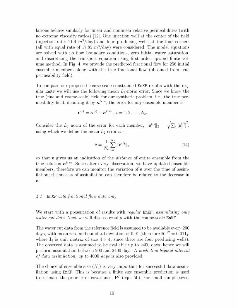
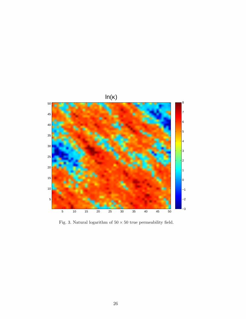
An initial ensemble with different permeability realizations was generated us-ing the sequential Gaussian simulation (SGSIM) 1 [7]. We specified a Gaussianvariogram model with a correlation length of 20 gridblocks in the x-directionand 5 gridblocks in the y-direction; one of the realizations is used as the ref-erence field (depicted in Fig. 3). The fractional flow will be calculated basedon the fine-scale model in Section 2.1. Porosity (φ) is assumed to be equal to0.15 for all grid blocks. For simplicity, relative permeabilities, krj are assumedto be linear functions of water saturation (S): krw(S) = S, kro(S) = 1 − S.We note that this linearity assumption does not affect our data assimilationresults. When single-phase upscaling (i.e., upscaling of absolute permeabilityonly) is used, the errors in water cuts between coarse- and fine-scale simu-
1 For reservoir simulation applications, the SGSIM has been used [23,8] for gener-ating initial ensemble members. This approach yields independent and identicallydistributed multivariate normal random fields (conditioned to well log data)
9
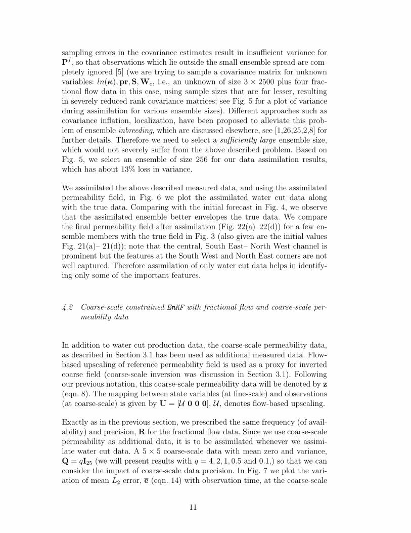
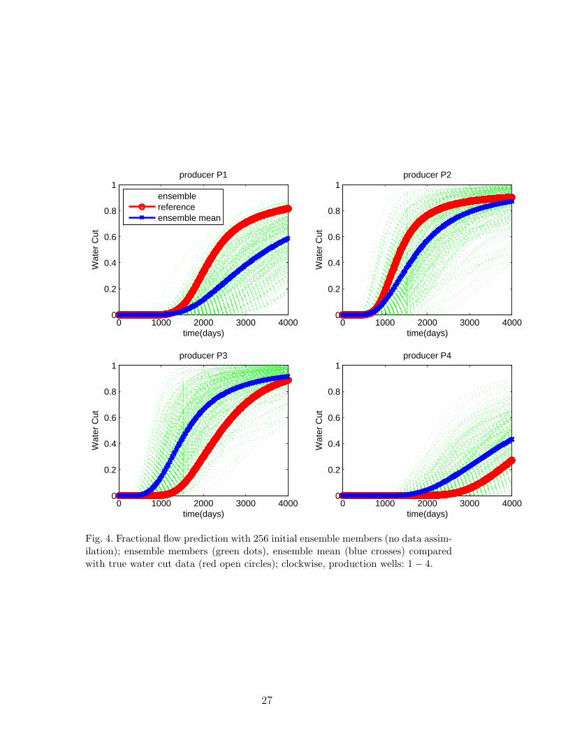
lations behave similarly for linear and nonlinear relative permeabilities (withno extreme viscosity ratios) [12]. One injection well at the center of the field(injection rate: 71.4 m3/day) and four producing wells at the four corners(all with equal rate of 17.85 m3/day) were considered. The model equationsare solved with no flow boundary conditions, zero initial water saturation,and discretizing the transport equation using first order upwind finite vol-ume method. In Fig. 4, we provide the predicted fractional flow for 256 initialensemble members along with the true fractional flow (obtained from truepermeability field).
To compare our proposed coarse-scale constrained EnKF results with the reg-ular EnKF we will use the following mean L2-norm error. Since we know thetrue (fine and coarse-scale) field for our synthetic problem, i.e., the true per-meability field, denoting it by κtrue, the error for any ensemble member is
e(i) = κ(i) − κtrue, i = 1, 2, . . . , Ne.
Consider the L2 norm of the error for each member, ‖e(i)‖2 =
√∑j [e
(i)j ]
2,
using which we define the mean L2 error as
e =1
Ne
Ne∑i=1
‖e(i)‖2, (14)
so that e gives us an indication of the distance of entire ensemble from thetrue solution κtrue. Since after every observation, we have updated ensemblemembers, therefore we can monitor the variation of e over the time of assim-ilation; the success of assimilation can therefore be related to the decrease ine.
4.1 EnKF with fractional flow data only
We start with a presentation of results with regular EnKF, assimilating onlywater cut data. Next we will discuss results with the coarse-scale EnKF.
The water cut data from the reference field is assumed to be available every 200days, with mean zero and standard deviation of 0.01 (therefore R1/2 = 0.01I4,where I4 is unit matrix of size 4 × 4, since there are four producing wells).The observed data is assumed to be available up to 2400 days, hence we willperform assimilation between 200 and 2400 days. A prediction beyond intervalof data assimilation, up to 4000 days is also provided.
The choice of ensemble size (Ne) is very important for successful data assim-ilation using EnKF. This is because a finite size ensemble prediction is usedto estimate the prior error covariance, Pf (eqn. 5b). For small sample sizes,
10
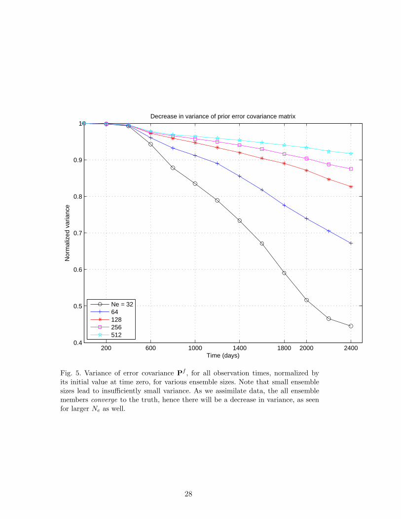
sampling errors in the covariance estimates result in insufficient variance forPf , so that observations which lie outside the small ensemble spread are com-pletely ignored [5] (we are trying to sample a covariance matrix for unknownvariables: ln(κ),pr,S,Wc, i.e., an unknown of size 3 × 2500 plus four frac-tional flow data in this case, using sample sizes that are far lesser, resultingin severely reduced rank covariance matrices; see Fig. 5 for a plot of varianceduring assimilation for various ensemble sizes). Different approaches such ascovariance inflation, localization, have been proposed to alleviate this prob-lem of ensemble inbreeding, which are discussed elsewhere, see [1,26,25,2,8] forfurther details. Therefore we need to select a sufficiently large ensemble size,which would not severely suffer from the above described problem. Based onFig. 5, we select an ensemble of size 256 for our data assimilation results,which has about 13% loss in variance.
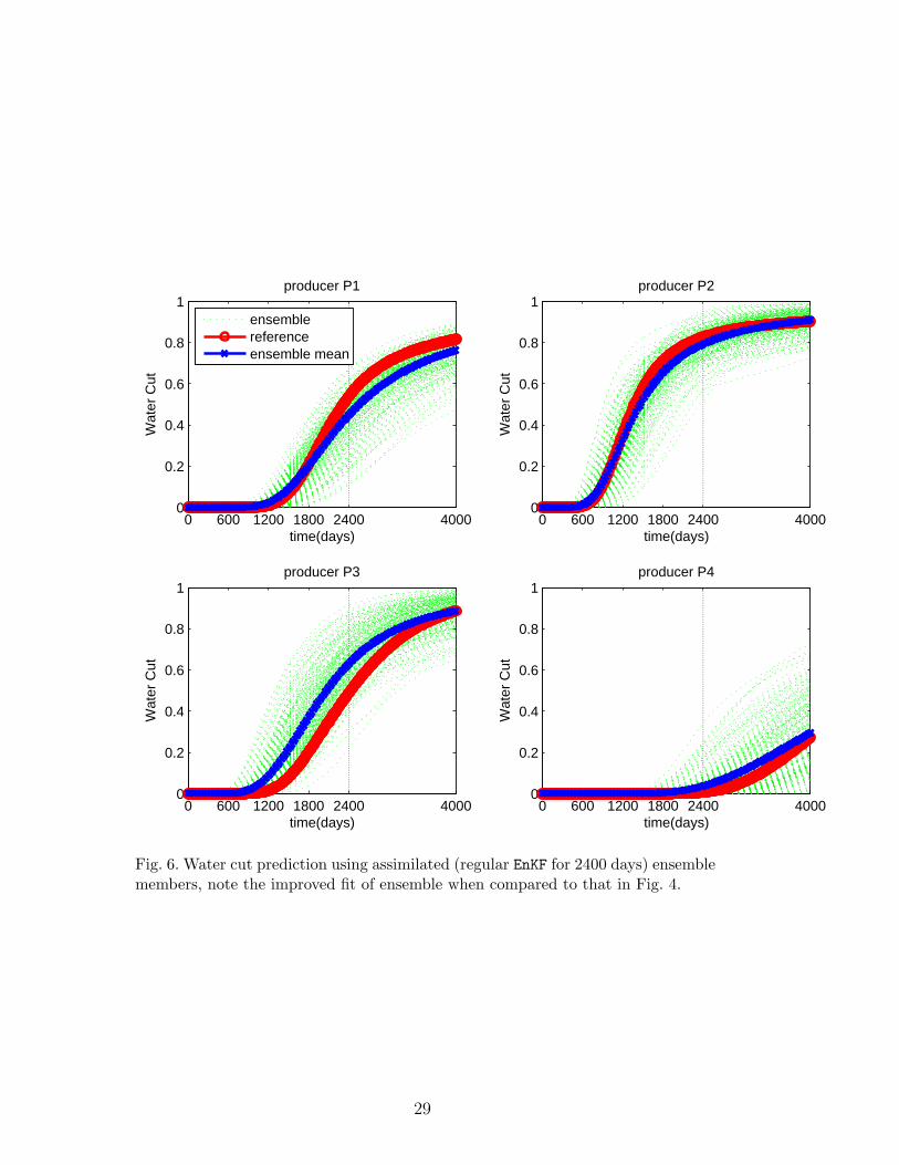
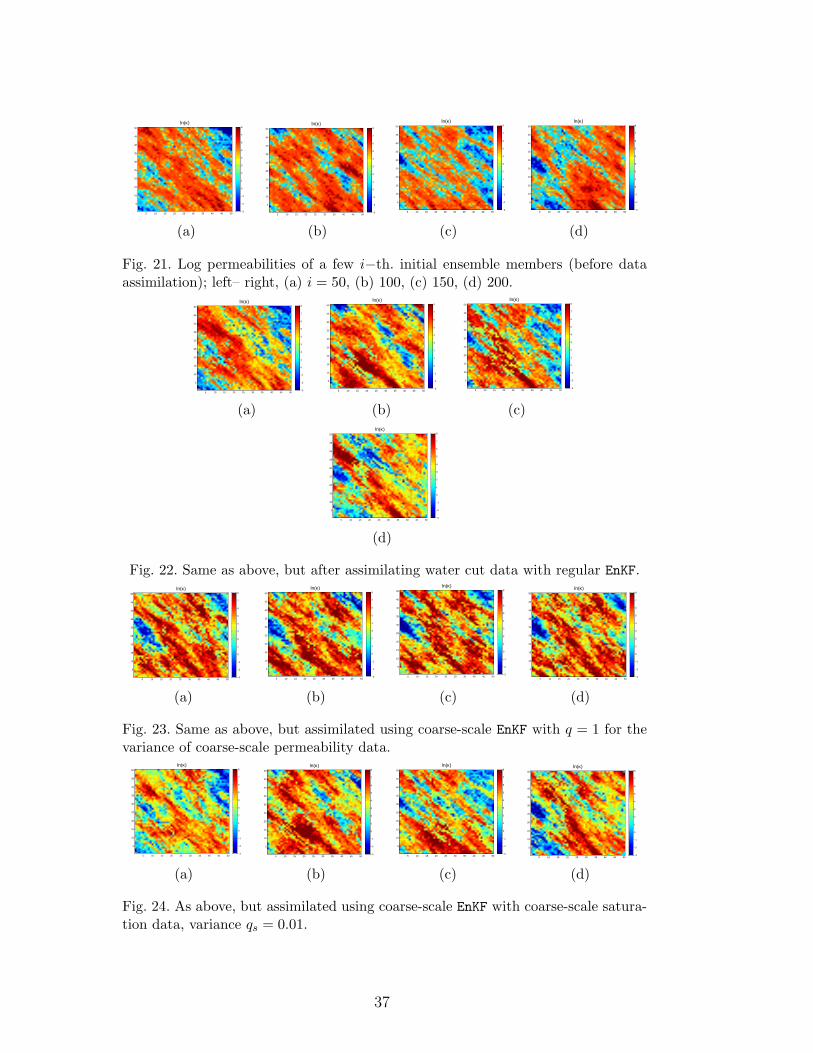
We assimilated the above described measured data, and using the assimilatedpermeability field, in Fig. 6 we plot the assimilated water cut data alongwith the true data. Comparing with the initial forecast in Fig. 4, we observethat the assimilated ensemble better envelopes the true data. We comparethe final permeability field after assimilation (Fig. 22(a)–22(d)) for a few en-semble members with the true field in Fig. 3 (also given are the initial valuesFig. 21(a)– 21(d)); note that the central, South East– North West channel isprominent but the features at the South West and North East corners are notwell captured. Therefore assimilation of only water cut data helps in identify-ing only some of the important features.
4.2 Coarse-scale constrained EnKF with fractional flow and coarse-scale per-meability data
In addition to water cut production data, the coarse-scale permeability data,as described in Section 3.1 has been used as additional measured data. Flow-based upscaling of reference permeability field is used as a proxy for invertedcoarse field (coarse-scale inversion was discussion in Section 3.1). Followingour previous notation, this coarse-scale permeability data will be denoted by z(eqn. 8). The mapping between state variables (at fine-scale) and observations(at coarse-scale) is given by U = [U 0 0 0], U , denotes flow-based upscaling.
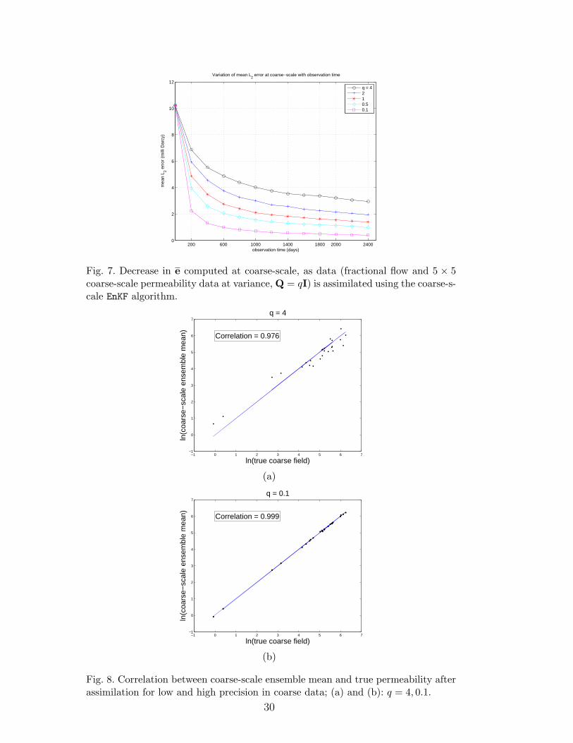
Exactly as in the previous section, we prescribed the same frequency (of avail-ability) and precision, R for the fractional flow data. Since we use coarse-scalepermeability as additional data, it is to be assimilated whenever we assimi-late water cut data. A 5 × 5 coarse-scale data with mean zero and variance,Q = qI25 (we will present results with q = 4, 2, 1, 0.5 and 0.1,) so that we canconsider the impact of coarse-scale data precision. In Fig. 7 we plot the vari-ation of mean L2 error, e (eqn. 14) with observation time, at the coarse-scale
11
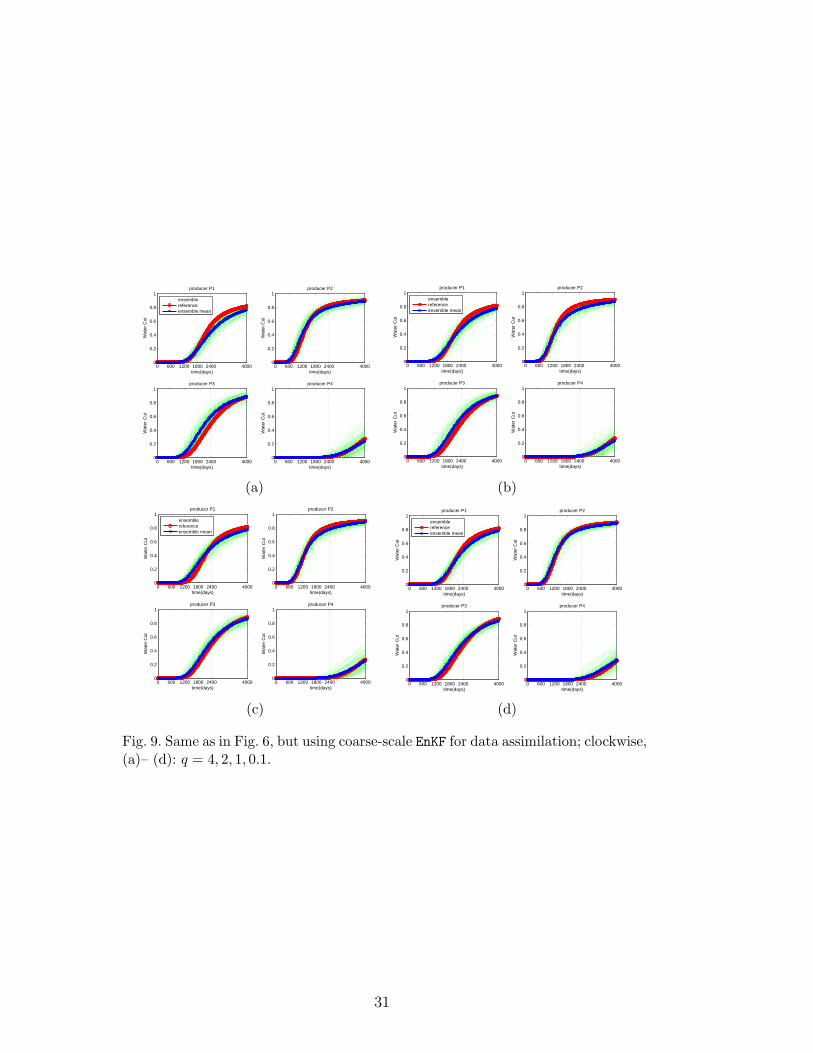
for different values of q. Figures 8(a) and 8(b) depict the correlation betweencoarse-scale ensemble mean and true fields for q = 4 and 0.1, respectively. Asthe precision of coarse-scale data is increased, i.e., for smaller variance, weobserve a larger decrease in coarse-scale mean L2 error and higher correlationwith true coarse-scale field (correlation coefficient for q = 4, 2, 1, 0.1 respec-tively are 0.976, 0.992, 0.995, 0.999), because smaller variance Q implies morestricter coarse-scale data constraint in eqn. (8). Fig. 9(a)–9(d) depict the frac-tional flow using the final permeability field after assimilation, for differentcoarse-scale data precisions. Fig. 7 and 8(a)–8(b) show that the coarse-scaledata is being more accurately assimilated as it is made more precise. Also, no-tice the improved fit of ensemble prediction to the true data, for more precisecoarse-scale data; also when compared to the regular EnKF results in Fig. 6.
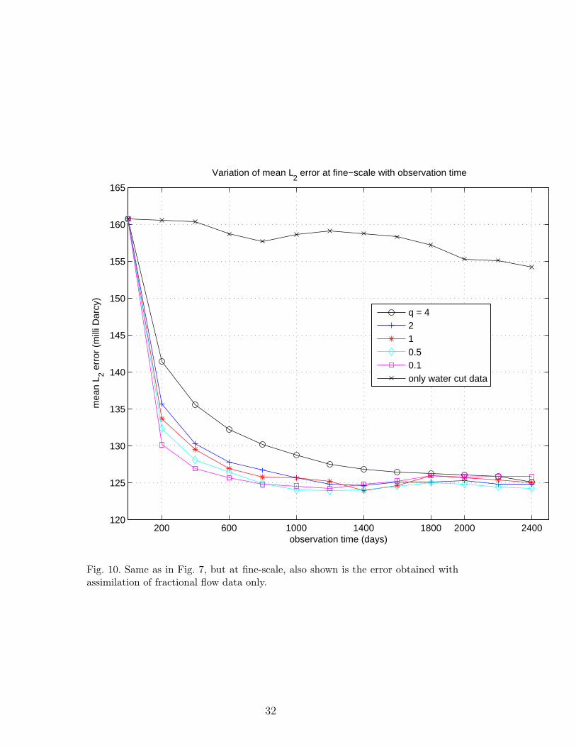
Now we discuss the results regarding fine-scale field. In Fig. 10 we plot thefine-scale mean L2 error for different values of q; the coarse-scale EnKF yieldsmuch lesser error than regular EnKF which assimilated only fractional flowdata. The correlation coefficient between fine-scale ensemble mean and truefields, after assimilating using regular EnKF is equal to 0.409, while with thecoarse-scale EnKF for q = 4, 2, 1, 0.1, in that order were 0.644, 0.652, 0.638, and0.626; note higher correlation with the coarse-scale EnKF. We observe thathigher precision, i.e., lower q does not necessarily imply least e or highestcorrelation, since highly precise coarse-scale data is relatively more weightedthan the fractional flow data. Optimal value for the coarse-scale data variancecan be obtained by prior calculation, which will be addressed in a future study.
The final permeability field, for a few ensemble members after assimilatingwith coarse-scale EnKF, for q = 1 is shown in figures 23(a)– 23(d); all shownsamples seem to be more closer to the true field (Fig. 3) than those obtainedwith regular EnKF (Fig. 22(a)–22(d)). In particular note that the low perme-ability region at the North East and high permeability at the South Westcorners are well captured.
4.3 Coarse-scale constrained EnKF with fractional flow and coarse-scale sat-uration data
As mentioned in the Introduction and Section 3.1, by coarse-scale inversion of4d-seismic data, we could obtain dynamic data such as coarse-scale pressureand saturation. In this section we will use our proposed coarse-scale EnKF al-gorithm to study the impact of usage of coarse-scale saturation as measureddata. To this end, the saturation obtained by using the reference permeability,is saved at three different times: 200, 1200 and 2400 days which correspond tothe start, middle and end of the time window of data assimilation. This savedfine-scale saturation field is then upscaled (see Section 3.1) by volume averag-
12
ing to a 5 × 5 coarse-scale grid and used as observed coarse-scale saturationdata. If we denote the volume averaging by operator A, acting on fine-scalesaturation Sf , to give coarse-scale saturation Sc = ASf , then the mapping be-tween state variables at fine-scale and measured data at coarse-scale is givenby U = [0 0 A 0]. Therefore in Steps 2.1 and 2.4, of the coarse-scale EnKF al-gorithm (Appendix B), we use this operator to compute the misfit: z−U[Ψ].Unlike the coarse-scale permeability data which is to be taken into accountat every assimilation step, by construction, the coarse-scale saturation data isavailable only at a few assimilation steps, in this particular case, assimilationafter 200, 1200 and 2400 days.
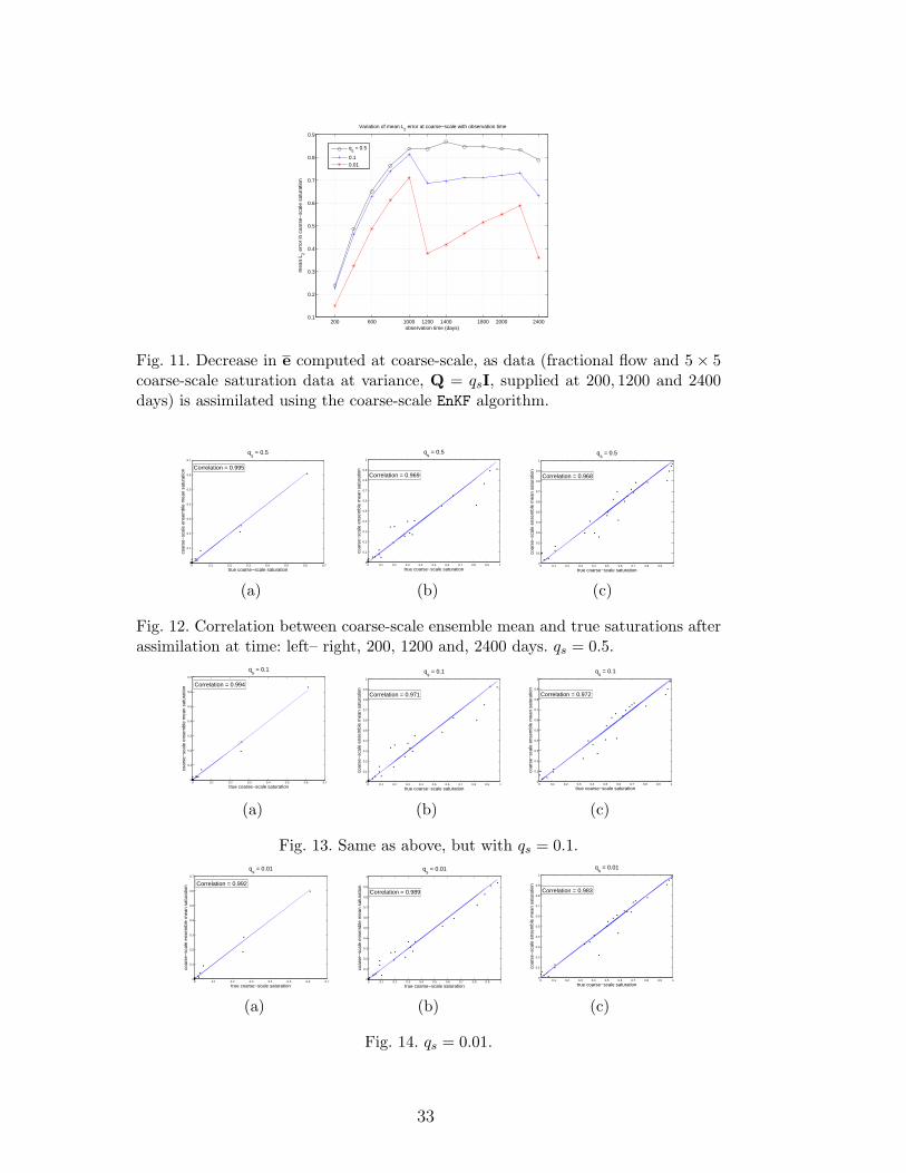
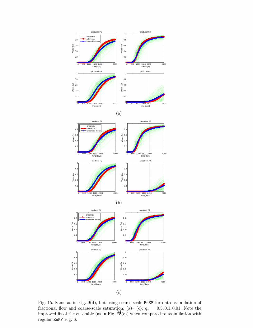
To be consistent with our previous results, the frequency (of availability) andprecision, R for the fractional flow data has been kept the same. The coarse-scale saturation data with mean zero and variance, Q = qsI25 (we will considerresults with qs = 0.5, 0.1, 0.01) such that the precision is varied from low- high.Since the saturation ranges between zero and one, and the fractional flowdata is usually more accurately measured than 4d-seismic data, we pickedqs to be always larger than the variance in fractional flow data. In Fig.11we plot the variation of mean L2 error for the coarse-scale saturation (whileassimilating) versus observation time (for our test case, we had assumed zeroinitial water saturation, therefore the water saturation increases with time,hence the inherent, increasing trend in Fig. 11). Note that whenever the coarse-scale saturation is assimilated the error decreases for all three values of qs.Oncethe data has been assimilated using the coarse-scale EnKF algorithm, we predictusing the assimilated ensemble members. The correlation of predicted coarse-scale saturation with the true coarse-scale field at 200, 1200 and 2400 days, fordifferent values of qs is given in figures 12(a)–14(c); note the higher correlationfor more precise coarse-scale data. The improved fit of the fractional flow dataprediction using the assimilated ensemble members is given in Fig.15(a)–15(c).For less precise data, such as qs = 0.5 : Fig.15(a), the results are somewhatsimilar to the regular EnKF results (Fig. 6), but as the precision is increased(qs = 0.01) the coarse-scale EnKF prediction is certainly improved and is closerto the truth.
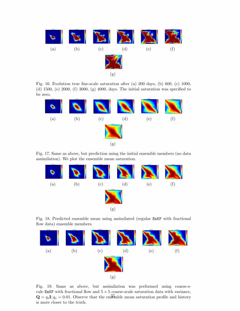
We discuss the fine-scale results, starting with fine-scale saturation and thenthe fine-scale permeability. The true fine-scale saturation at certain times, isplotted in Fig. 16(a)–16(g). The mean saturation with initial ensemble mem-bers (before data assimilation) is given in Fig. 17(a)–17(g) and Fig. 18(a)–18(g) show the field after assimilating only fractional flow data using regu-lar EnKF. Using the coarse-scale EnKF, with qs = 0.01 is shown in Figures 19(a)–19(g). Note that we are able to capture many of the subtle features that arepresent in the true saturation field, such as the fingers that develop off the cen-ter toward the North East corner and sharp contrast between different levels ofsaturation, throughout the entire time interval (up to 4000 days) considered.
13
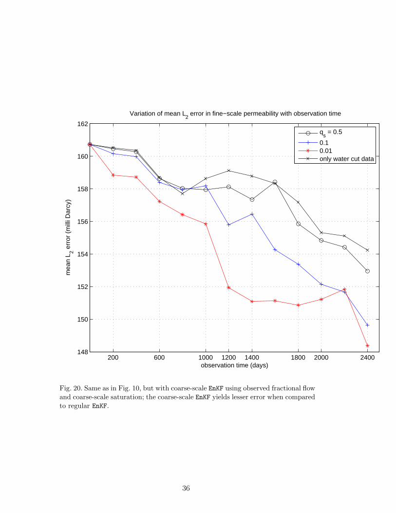
Next we discuss the fine-scale permeability results after assimilation with ourcoarse-scale EnKF. A comparison of the mean L2 error for the fine-scale perme-ability field for varying qs and that obtained using the regular EnKF is shownin Fig. 20. Note that the error variation with qs = 0.5 is very close to that withregular EnKF , which probably explains why the fractional flow (Fig. 15(a)) isnot much different from the assimilation of water cut data only (regular EnKF).Similarly improved results with qs = 0.01 could be explained based on smallestmean L2 error for the fine-scale permeability. Finally the fine-scale permeabil-ity field for a few ensemble members is plotted in Fig. 24(a)–24(d). Notice thatthough the South East– North West features are captured, unlike the resultsobtained with coarse-scale permeability data (Fig. 23(a)– 23(d)), the SouthWest and North East features are not well represented. In general the resultswith coarse-scale permeability data are better, in terms of fine-scale meanL2 error decrease and permeability samples, when compared to usage coarse-scale saturation data, which is anticipated, since the fine scale permeabilityis more correlated to coarse-scale permeability than coarse-scale saturation.Also, these results highlight the importance of accurate coarse-scale data andmodeling, since more accurate measurements lead to further decrease in un-certainty at the fine-scale.
5 Coarse-Scale Inversion
We assume that the observed water cut data corresponds to the model’ s finestscale response. This relationship will be written as,
yof (tn) =Mf (tn)[κtrue
f ], (15)
where yof (tn) is the observed water cut, superscript ‘o′ denotes observed data,
subscript ‘f ′, fine-scale and tn, the time step. The fine-scale model and truepermeability are respectively denoted byMf and κtrue
f . Once κtruef is upscaled,
we get κtruec , which could be used to obtain the so-called coarse-scale water
cut,y∗c (tn) =Mc(tn)[κtrue
c ], (16)
using the coarse-scale model, Mc. Hence to obtain the coarse-scale true per-meability, κtrue
c , we first need to generate coarse-scale water cut data thatcorresponds to the reference fine-scale water cut. This coarse-scale data couldthen be inverted to obtain the coarse-scale field, for e.g., using coarse-scalegradient sensitivity [37]; here we will instead use regular EnKF algorithm on acoarse-grid and, sequentially estimate the coarse-scale permeability field. Theassimilated coarse-scale ensemble mean permeability obtained after a certainnumber of days could then be used as a constraint for coarse-scale EnKF de-scribed in section 4.2. In other words, this methodology could be used toobtain coarse-scale permeability data, using the observed water cut data, say
14
between time: [t1, t2], 0 < t1 < t2. Then we can use coarse-scale permeabilityand observed water cut within (t2, T ], for coarse-scale EnKF (the final watercut observation is at time, T ). However, the first step is to obtain the coarse-scale production data (which will be denoted by yc(tn)) using the observedfine-scale data, yo
f (tn).
5.1 Fine-scale to coarse-scale production map
Using an ensemble of fine-scale fields: κ(i)f , i = 1, Ne, we obtain correspond-
ing fine-scale water cut, y(i)f (tn) = Mf (tn)[κ
(i)f ]. By single phase flow based
upscaling of fine-scale ensemble permeability fields we obtain, κ(i)c , i = 1, Ne.
Therefore using the coarse-scale model, we get y(i)c (tn) = Mc(tn)[κ(i)
c ], suchthat at any time step, tn, for every fine-scale fractional flow data value, thereis a corresponding coarse-scale image point. In Fig. 25, we plot for an arbi-trary ensemble member the fine and coarse-scale fractional flow curves, withthe same configuration of wells as earlier including the fine and coarse-scalegrid sizes, namely, 50 × 50 and 5 × 5 respectively. A plot of fine-scale versuscoarse-scale water cut for one of the four producers at the end of 3000 days isshown in Fig. 26 with Ne = 100 realizations. Given the discrete sets: y(i)
f (tn)and y(i)
c (tn), here we adopt a simple linear least-squares approach to obtaincoarse-scale water cut, yc(tn) correspoding to observed fine scale data, yo
f (tn).We start by writing any coarse-scale fractional flow value as,
y(i)c (tn) = α(tn)y
(i)f (tn) + β(tn), (17)
where α(tn) and β(tn) are scalar coefficients. Least-squares fit values (α∗(tn)and β∗(tn)) of these parameters are obtained by minimizing,
Ne∑i=1
(y(i)c − αy
(i)f − β)2
at every tn (a similar approach was studied by Omre and Lødøen [33] tomodel a mapping of coarse-scale to fine-scale water cut). Therefore yc(tn) =α∗(tn)yo
f (tn)+β∗(tn) and, could be seen as an approximation to y∗c (tn), the truecoarse-scale water cut (eqn.16). This off-line method therefore relies on a num-ber of fine and coarse-scale simulations. As mentioned in section 2.1, coarse-scale simulation is relatively inexpensive when compared to the compuationalcost of a corresponding fine-scale simulation and since this entire procedurecan be implemented offline, it is affordable. Moreover, for our results we mapthe observed fractional flow only in the early time period, to obtain yc. Thesame fine-scale reference field as earlier in Section 4 (Fig. 3), when upscaled(flow based) yields coarse-scale field, when used in coarse-scale simulation pro-vides y∗c . The observed fractional flow data, yo
f , is also the same as used earlier,
15
for e.g., in regular EnKF, Section 4.1. A comparison of yc (obtained from abovedescribed mapping of yo
f ) and y∗c is given in Fig. 27. The mapped coarse-scalefractional flow, yc deviates slightly from y∗c , however, this could be minimizedby considering a larger sample size and/or a different fit other than the linearfit, to be studied in future research work.
5.2 EnKF on coarse-grid
Our goal is to sequentially estimate coarse-scale state (including coarse-scalepermeability) using the above obtained coarse-scale water cut. The regu-lar EnKF algorithm is implemented for the coarse-scale permeability samples,κ(i)
c , i = 1, Ne and yc, as coarse-scale observed data. This can be accomplishedwith minimal computational resources since the size of the coarse-grid is rel-atively much smaller than the fine-scale grid. Because upscaled permeabilityfields are used for imposing a constraint in EnKF, we can also use MCMC tech-niques (e.g., [16]) to obtain coarse-scale permeability samples conditioned towater-cut data. In Fig. 28 we compare the assimilated coarse-scale ensemblemean permeability with the reference coarse-scale field (flow upscaled fine-scale permeability). We observed that the ensemble mean coarse-scale perme-ability after coarse grid data assimilation, is approximately the same as coarse-scale permeability field obtained by flow-based upscaling of the fine-scale ref-erence permeability field. As a result, we observed that coarse-scale EnKF givessimilar results to those presented earlier (in Section 4.2), which used flow-basedupscaling of the fine-scale reference permeability field.
6 Conclusions
The EnKF is increasingly being used for subsurface characterization in variousgeological and groundwater applications to identify fine-scale state and pa-rameters. So far, various implementations have been based on using dynamic,production data, such as water cut, well pressures, etc, for sequential data as-similation. Only recently dynamic data other than production data has beenconsidered in the EnKF context ([9,34]), nevertheless the observed data to beassimilated was assumed to be at the finest scale. For a number of reasons,it is widely recognized that usage of additional multiscale data could furtherreduce the uncertainty at the fine scale. This is further motivated by the in-creasing popularity of coarse-scale modeling. In this light, here we proposedassimilation of coarse-scale data along with water cut, production data us-ing coarse-scale EnKF. The modification to the regular EnKF (assimilation ofonly water cut data) is completely recursive and easily implementable. Therelation between fine and coarse scales has been modeled via physics based
16
upscaling, which could be thought of as a nonlinear observation operator link-ing the coarse-scale data to the unknown fine-scale variables. In addition, theproposed methodology could be used in any other sequential data assimilationmethod as well.
The coarse-scale EnKF was tested and compared with the regular EnKF for a2D synthetic 50× 50 heterogenuous true field. Two kinds of coarse-scale datawere considered. In the first implementation, coarse-scale permeability datawas considered. In the second, we considered volume averaged coarse-scalesaturation from the reference case as coarse-scale data; in both cases, a 5× 5coarse grid was used. The coarse-scale saturation was assimilated only threetimes in the entire time window of data assimilation (beginning, middle andend). Therefore unlike coarse-scale permeability data which was always as-similated along with water cut data, coarse-scale saturation was only thriceassimilated. The data variance was varied from low to high, to study its im-pact on assimilated results. In all cases, we observed that the assimilated,ensemble mean coarse-scale field for all variances was highly correlated tothe true coarse-scale field. In addition, lower variance in the coarse-scale datayielded higher correlation. The water cut data was better honored, both forhigher precision of coarse data, and when compared with regular EnKF. Asfor the fine-scale permeability field, the coarse-scale EnKF yielded lesser errorin an averaged L2 norm, error taken w.r.t. the reference field. In addition,a few individual samples were picked to compare the assimilated fields withdifferent EnKF procedures; experiment with coarse-scale permeability data pro-vided final samples which captured most closely the features in the referencefine-scale field. We also compared the fine-scale water saturation profile fordifferent times, a comparison with the regular EnKF showed that the profilewith coarse-scale EnKF (with coarse saturation) replicated many of the subtlefeatures present in the true saturation profile.
Though in our current paper we used only one coarse-scale, the proposedmethod can be easily implemented to integrate as many scales as required bythe available data. We also discussed an alternative method to obtain coarse-scale permeability data, if it was not available from prior geological considera-tion. This procedure was based on first modeling an approximate relationshipbetween fine- and coarse-scale fractional flows. The mapped coarse-scale frac-tional flow was then used in sequential estimation of coarse-scale permeability.Our results indicated that the estimated coarse-scale ensemble mean perme-ability is similar to the one obtained via a flow-based upscaling of the fine-scalereference field.
Our current and future work is directed toward assimilating observations atmultiple scales into three dimensional models.
APPENDIX A Two step coarse-scale constrained Kalman filter es-
17
timate
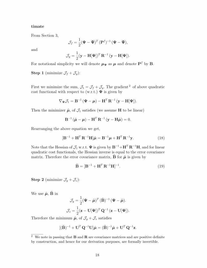
From Section 3,
Jf =1
2(Ψ−Ψ)T (Pf )−1 (Ψ−Ψ),
and
Jy =1
2(y−H[Ψ])T R−1 (y−H[Ψ]).
For notational simplicity we will denote µΨ as µ and denote Pf by B.
Step 1 (minimize Jf + Jy):
First we minimize the sum, J1 = Jf + Jy. The gradient 2 of above quadraticcost functional with respect to (w.r.t.) Ψ is given by
∇ΨJ1 = B−1 (Ψ− µ)−HT R−1 (y−H[Ψ]).
Then the minimizer µ, of J1 satisfies (we assume H to be linear)
B−1 (µ− µ)−HT R−1 (y−Hµ) = 0.
Rearranging the above equation we get,
[B−1 + HT R−1H]µ = B−1µ+ HT R−1y. (18)
Note that the Hessian of J1 w.r.t. Ψ is given by B−1+HT R−1H, and for linearquadratic cost functionals, the Hessian inverse is equal to the error covariancematrix. Therefore the error covariance matrix, B for µ is given by
B = [B−1 + HT R−1H]−1. (19)
Step 2 (minimize Jg + Jz):
We use µ, B in
Jg =1
2(Ψ− µ)T (B)−1 (Ψ− µ).
Jz =1
2(z−U[Ψ])T Q−1 (z−U[Ψ]).
Therefore the minimum µ, of Jg + Jz satisfies
[(B)−1 + UT Q−1U]µ = (B)−1µ+ UT Q−1z.
2 We note in passing that B and R are covariance matrices and are positive definiteby construction, and hence for our derivation purposes, are formally invertible.
18
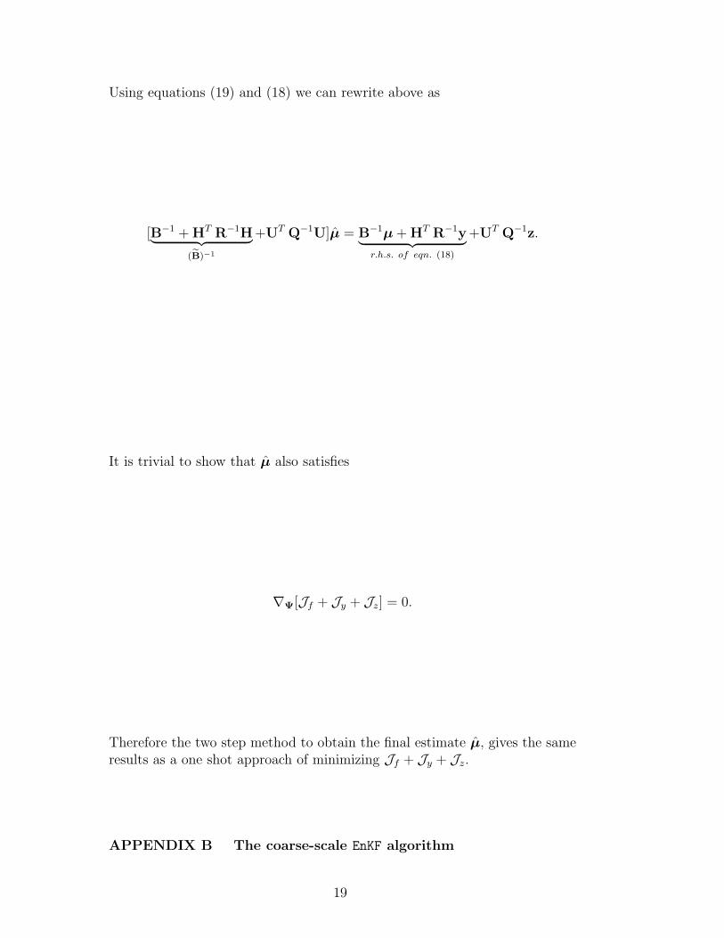
Using equations (19) and (18) we can rewrite above as
[B−1 + HT R−1H︸ ︷︷ ︸(B)−1
+UT Q−1U]µ = B−1µ+ HT R−1y︸ ︷︷ ︸r.h.s. of eqn. (18)
+UT Q−1z.
It is trivial to show that µ also satisfies
∇Ψ[Jf + Jy + Jz] = 0.
Therefore the two step method to obtain the final estimate µ, gives the sameresults as a one shot approach of minimizing Jf + Jy + Jz.
APPENDIX B The coarse-scale EnKF algorithm
19
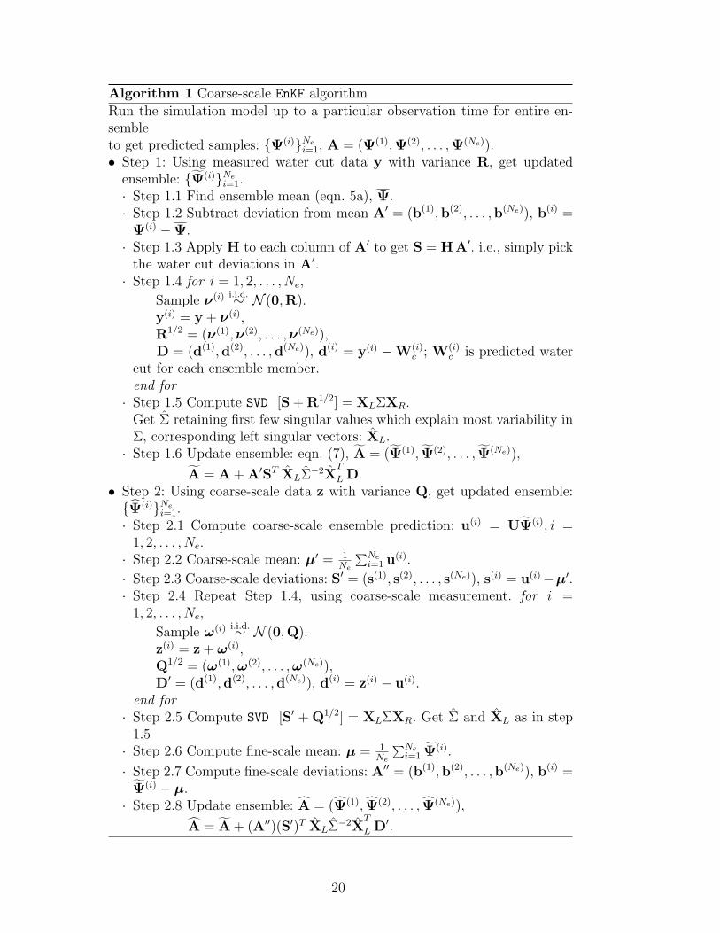
Algorithm 1 Coarse-scale EnKF algorithm
Run the simulation model up to a particular observation time for entire en-sembleto get predicted samples: Ψ(i)Ne
i=1, A = (Ψ(1),Ψ(2), . . . ,Ψ(Ne)).• Step 1: Using measured water cut data y with variance R, get updated
ensemble: Ψ(i)Nei=1.
· Step 1.1 Find ensemble mean (eqn. 5a), Ψ.· Step 1.2 Subtract deviation from mean A′ = (b(1),b(2), . . . ,b(Ne)), b(i) =
Ψ(i) −Ψ.· Step 1.3 Apply H to each column of A′ to get S = H A′. i.e., simply pick
the water cut deviations in A′.· Step 1.4 for i = 1, 2, . . . , Ne,
Sample ν(i) i.i.d.∼ N (0,R).y(i) = y + ν(i),R1/2 = (ν(1),ν(2), . . . ,ν(Ne)),D = (d(1),d(2), . . . ,d(Ne)), d(i) = y(i) −W(i)
c ; W(i)c is predicted water
cut for each ensemble member.end for· Step 1.5 Compute SVD [S + R1/2] = XLΣXR.
Get Σ retaining first few singular values which explain most variability inΣ, corresponding left singular vectors: XL.· Step 1.6 Update ensemble: eqn. (7), A = (Ψ(1), Ψ(2), . . . , Ψ(Ne)),
A = A + A′ST XLΣ−2XT
L D.• Step 2: Using coarse-scale data z with variance Q, get updated ensemble:Ψ(i)Ne
i=1.· Step 2.1 Compute coarse-scale ensemble prediction: u(i) = UΨ(i), i =
1, 2, . . . , Ne.· Step 2.2 Coarse-scale mean: µ′ = 1
Ne
∑Nei=1 u(i).
· Step 2.3 Coarse-scale deviations: S′ = (s(1), s(2), . . . , s(Ne)), s(i) = u(i)−µ′.· Step 2.4 Repeat Step 1.4, using coarse-scale measurement. for i =
1, 2, . . . , Ne,
Sample ω(i) i.i.d.∼ N (0,Q).z(i) = z + ω(i),Q1/2 = (ω(1),ω(2), . . . ,ω(Ne)),D′ = (d(1),d(2), . . . ,d(Ne)), d(i) = z(i) − u(i).
end for· Step 2.5 Compute SVD [S′ + Q1/2] = XLΣXR. Get Σ and XL as in step
1.5· Step 2.6 Compute fine-scale mean: µ = 1
Ne
∑Nei=1 Ψ(i).
· Step 2.7 Compute fine-scale deviations: A′′ = (b(1),b(2), . . . ,b(Ne)), b(i) =Ψ(i) − µ.· Step 2.8 Update ensemble: A = (Ψ(1), Ψ(2), . . . , Ψ(Ne)),
A = A + (A′′)(S′)T XLΣ−2XT
L D′.
20
Remark 1:Note that steps 2.6 and 2.7 in above algorithm approximate the intermediatefine-scale error covariance
Pf ≈ 1
Ne − 1A′′ (A′′)T .
Remark 2:Steps 2.1– 2.3 accomplish 3
S′ = UA′′.
Note that the above algorithm is independent of the choice of upscaling proce-dure and also, we can use the same algorithm for different kinds of coarse-scaleobserved data (if available).
Remark 3:Note that the above coarse-scale constrained EnKF algorithm can be readilyextended to incorporate data at multiple coarse scales, with appropriate up-scaling procedure in U. To elaborate, if we had another independent data ata scale different from z, we use the estimates (Ψ(i)Ne
i=1) obtained using z, asintermediate solution, repeat Step 2 to assimilate the data at another scale.
References
[1] Anderson JL. Exploring the need for localization in ensemble data assimilationusing a hierarchical ensemble filter. Physica D 2007; 230(1-2): 99–111.
[2] Arroyo-Negrete E, Devegowda D, Datta-Gupta A, Choe J. Continuous reservoirmodel updating using streamline assisted ensemble Kalman filter. SPE AnnualTechnical Conference and Exhibition, 24-27 September 2006, San Antonio,Texas, USA; 106518-STU.
[3] Barker JW, Thibeau S. A critical review of the use of pseudo-relativepermeabilities for upscaling, SPE Res. Eng. 1997; 12: 138–143.
[4] Burgers G, van Leeuwen PJ, Evensen G. Analysis scheme in the ensembleKalman filter. Monthly Weather Review 1998; 126(6): 1719-1724.
[5] Chen Y, Zhang D. Data assimilation for transient flow in geologic formationsvia ensemble Kalman filter. Advances in Water Resources 2006; 29: 1107-1122.
[6] Christie M. Upscaling for reservoir simulation. J. Pet. Tech. 1996; 1004–1010.
[7] Deutsch CV, Journel A. GSLIB Geostatistical Software Library and User‘ sGuide. Oxford Univ. Press, 1992.
3 As noted in [21], this approach of accounting for nonlinear observations operatorU, works well, as long as U is weakly nonlinear and a monotonic function of modelvariables Ψ
21
[8] Devegowda D, Arroyo-Negrete E, Datta-Gupta A. Efficient and robust reservoirmodel updating using ensemble Kalman filter with sensitivity-based covariancelocalization. SPE Reservoir Simulation Symposium held in Houston, TX, 26-28February 2007; 106144-MS.
[9] Dong Y, Gu Y, Oliver DS. Sequential assimilation of 4D seismic data forreservoir description using the ensemble kalman filter. Journal of PetroleumScience and Engineering 2006; 53: 83- 99.
[10] Durlofsky LJ. Numerical calculation of equivalent grid block permeabilitytensors for heterogeneous porous media. Water Resour. Res. 1991; 27: 699–708.
[11] Durlofsky LJ. Coarse scale models of two phase flow in heterogeneous reservoirs:Volume averaged equations and their relationship to the existing upscalingtechniques. Computational Geosciences 1998; 2: 73–92.
[12] Durlofsky LJ, Behrens RA, Jones RC, Bernath A. Scale up of heterogeneousthree dimensional reservoir descriptions. SPE paper 30709, 1996.
[13] Durlofsky LJ, Jones RC, Milliken WJ. A nonuniform coarsening approach forthe scale up of displacement processes in heterogeneous media. Advances inWater Resources 1997; 20: 335–347.
[14] Efendiev Y, Datta-Gupta A, Ginting V, Ma X, Mallick B. An efficient two-stage Markov chain Monte Carlo method for dynamic data integration. WaterResources Research 2005; 41: W12423.
[15] Efendiev Y, Datta-Gupta A, Osako I, Mallick B. Multiscale data integrationusing coarse-scale models. Advances in Water Resources 2005; 28:303- 314.
[16] Efendiev Y, Datta-Gupta A, Ginting V, Ma X, Mallick B. An efficient two-stage Markov chain Monte Carlo methods for dynamic data integration. WaterResources Research, 41, W12423, doi:=10.1029/2004WR003764
[17] Efendiev Y, Durlofsky L. Generalized convection-diffusion model for subgridtransport in porous media. SIAM Multiscale Modeling and Simulation 2003; 1:504526.
[18] Efendiev Y, Durlofsky L. Accurate subgrid models for two-phase flow inheterogeneous reservoirs. SPE Journal 2004; 9: 219-226.
[19] Efendiev YR, Durlofsky LJ. Numerical modeling of subgrid heterogeneity intwo phase flow simulations. Water Resour. Res. 2002; 38(8): W1128.
[20] Evensen G. Sequential data assimilation with a nonlinear quasi-geostrophicmodel using Monte Carlo methods to forecast error statistics. Journal ofGeophysical Research 1994; 99(10), 14310, 162.
[21] Evensen G. Data Assimilation: The Ensemble Kalman Filter. Springer, 2006.
[22] Gosselin O, Aanonsen SI, Aavatsmark I, Cominelli A, Gonard R, Kolasinski M,Ferdinandi F, Kovacic L, Neylon K. History matching using time-lapse seismic(HUTS). SPE Annual Technical Conference and Exhibition, Denver 58 October2003; SPE 84464-MS.
22
[23] Gu Y, Oliver DS. History Matching of the PUNQ-S3 reservoir model using theensemble Kalman filter. SPE Journal 2005; 10: 217- 224.
[24] Gu YQ, Oliver DS. The ensemble kalman filter for continuous updatingof reservoir simulation models. Journal of Energy Resources Technology-Transactions of the ASME 2006; 128: 79- 87.
[25] Hamill T, Whitaker J, Synder C. Distance-Dependent filtering of backgrounderror covariance estimates in ensemble Kalman filter. Monthly Weather Review2001; 129: 2776- 2790.
[26] Houtekamer P, Mitchell H. A sequential ensemble kalman filter for atmosphericdata assimilation. Monthly Weather Review 2001; 129: 123-137.
[27] Lee SH, Malallah A, Datta-Gupta A, Higdon D. Multiscale data integrationusing Markov random fields. SPE Reservoir Evaluation Engineering 2002; 5(1):68- 78.
[28] Lewis JM, Lakshmivarahan S, Dhall S. Dynamic Data Assimilation: ALeast Squares Approach (Encyclopedia of Mathematics and its Applications).Cambridge University Press, 2006.
[29] Liu Y, Gupta HV. Uncertainty in hydrologic modeling: Toward and integrateddata assimilation framework. Water Resources Research 2007; 43: W07401.
[30] Lumley DE. Time-lapse seismic reservoir monitoring. Geophysics 2001; 66: 50-53.
[31] Moradkhani H, Sorooshian S, Gupta H, Houser PR. Dual stateparameterestimation of hydrological models using ensemble Kalman filter. Advances inWater Resources 2005; 28: 135- 147.
[32] Nævdal G, Johnson L, Aanonsen S, Vefring E. Reservoir monitoring andcontinuous model updating using ensemble Kalman filter. SPE Journal 2005;10: 66- 74.
[33] Omre H, Lødøen OP. Improved production forecasts and history matching usingapproximate fluid-flow simulators. SPE Journal 2004; 9: 339– 351.
[34] Skjervheim J.-A, Evensen G, Aanonsen S, Ruud B, Johansen T. Incorporating4D seismic data in reservoir simulation models using ensemble Kalman filter.SPE Journal 2007; 12: 282- 292.
[35] Wen X.-H, Chen WH. Real-time reservoir model updating using ensembleKalman filter. SPE Reservoir Simulation Symposium 2005; SPE 92991.
[36] Wu XH, Efendiev YR, Hou TY. Analysis of upscaling absolute permeability.Discrete and Continuous Dynamical Systems, Series B 2002; 2: 185– 204.
[37] Yoon S, Malallah AH, Datta-Gupta A, Vasco DW, Behrens RA. A Multiscaleapproach to production-data integration using streamline models. SPE Journal2001; 6: 182– 192.
23
Ωc
Ωc
φ=0φ=1
no flow
no flow
div(κ(x)∇ φ)=0
Fig. 1. Schematic description of the upscaling. Bold lines illustrate a coarse-scalepartitioning, while thin lines show a fine-scale partitioning within coarse-grid cells.
24
Generate initial ensemble members
Predict entire ensemble up to observation time
Assimilate observed water cut data: step 1 of coarse-scale EnKF algorithm
Is there observed coarse-scale data ?
Assimilate coarse-scale data: step 2 of coarse-scale EnKF algorithm
yes
No
Additional Observations available ?
yes
No
Exit
Fig. 2. Coarse-scale EnKF algorithm
25
ln(κ)
5 10 15 20 25 30 35 40 45 50
5
10
15
20
25
30
35
40
45
50
−3
−2
−1
0
1
2
3
4
5
6
7
8
Fig. 3. Natural logarithm of 50× 50 true permeability field.
26
0 1000 2000 3000 40000
0.2
0.4
0.6
0.8
1producer P1
time(days)
Wat
er C
ut
0 1000 2000 3000 40000
0.2
0.4
0.6
0.8
1producer P2
time(days)
Wat
er C
ut
0 1000 2000 3000 40000
0.2
0.4
0.6
0.8
1producer P3
time(days)
Wat
er C
ut
0 1000 2000 3000 40000
0.2
0.4
0.6
0.8
1producer P4
time(days)
Wat
er C
ut
ensemblereferenceensemble mean
Fig. 4. Fractional flow prediction with 256 initial ensemble members (no data assim-ilation); ensemble members (green dots), ensemble mean (blue crosses) comparedwith true water cut data (red open circles); clockwise, production wells: 1− 4.
27
200 600 1000 1400 1800 2000 24000.4
0.5
0.6
0.7
0.8
0.9
1Decrease in variance of prior error covariance matrix
Nor
mal
ized
var
ianc
e
Time (days)
Ne = 3264128256512
Fig. 5. Variance of error covariance Pf , for all observation times, normalized byits initial value at time zero, for various ensemble sizes. Note that small ensemblesizes lead to insufficiently small variance. As we assimilate data, the all ensemblemembers converge to the truth, hence there will be a decrease in variance, as seenfor larger Ne as well.
28
0 600 1200 1800 2400 40000
0.2
0.4
0.6
0.8
1producer P1
time(days)
Wat
er C
ut
0 600 1200 1800 2400 40000
0.2
0.4
0.6
0.8
1producer P2
time(days)
Wat
er C
ut
0 600 1200 1800 2400 40000
0.2
0.4
0.6
0.8
1producer P3
time(days)
Wat
er C
ut
0 600 1200 1800 2400 40000
0.2
0.4
0.6
0.8
1producer P4
time(days)
Wat
er C
ut
ensemblereferenceensemble mean
Fig. 6. Water cut prediction using assimilated (regular EnKF for 2400 days) ensemblemembers, note the improved fit of ensemble when compared to that in Fig. 4.
29
200 600 1000 1400 1800 2000 24000
2
4
6
8
10
12
Variation of mean L2 error at coarse−scale with observation time
observation time (days)
mea
n L 2 e
rror
(m
illi D
arcy
)
q = 4210.50.1
Fig. 7. Decrease in e computed at coarse-scale, as data (fractional flow and 5 × 5coarse-scale permeability data at variance, Q = qI) is assimilated using the coarse-s-cale EnKF algorithm.
−1 0 1 2 3 4 5 6 7−1
0
1
2
3
4
5
6
7
ln(true coarse field)
ln(c
oars
e−sc
ale
ense
mbl
e m
ean)
q = 4
Correlation = 0.976
(a)
−1 0 1 2 3 4 5 6 7−1
0
1
2
3
4
5
6
7
ln(true coarse field)
ln(c
oars
e−sc
ale
ense
mbl
e m
ean)
q = 0.1
Correlation = 0.999
(b)
Fig. 8. Correlation between coarse-scale ensemble mean and true permeability afterassimilation for low and high precision in coarse data; (a) and (b): q = 4, 0.1.
30
0 600 1200 1800 2400 40000
0.2
0.4
0.6
0.8
1producer P1
time(days)
Wat
er C
ut
0 600 1200 1800 2400 40000
0.2
0.4
0.6
0.8
1producer P2
time(days)
Wat
er C
ut
0 600 1200 1800 2400 40000
0.2
0.4
0.6
0.8
1producer P3
time(days)
Wat
er C
ut
0 600 1200 1800 2400 40000
0.2
0.4
0.6
0.8
1producer P4
time(days)
Wat
er C
ut
ensemblereferenceensemble mean
(a)
0 600 1200 1800 2400 40000
0.2
0.4
0.6
0.8
1producer P1
time(days)
Wat
er C
ut
0 600 1200 1800 2400 40000
0.2
0.4
0.6
0.8
1producer P2
time(days)
Wat
er C
ut
0 600 1200 1800 2400 40000
0.2
0.4
0.6
0.8
1producer P3
time(days)
Wat
er C
ut
0 600 1200 1800 2400 40000
0.2
0.4
0.6
0.8
1producer P4
time(days)
Wat
er C
ut
ensemblereferenceensemble mean
(b)
0 600 1200 1800 2400 40000
0.2
0.4
0.6
0.8
1producer P1
time(days)
Wat
er C
ut
0 600 1200 1800 2400 40000
0.2
0.4
0.6
0.8
1producer P2
time(days)
Wat
er C
ut
0 600 1200 1800 2400 40000
0.2
0.4
0.6
0.8
1producer P3
time(days)
Wat
er C
ut
0 600 1200 1800 2400 40000
0.2
0.4
0.6
0.8
1producer P4
time(days)
Wat
er C
ut
ensemblereferenceensemble mean
(c)
0 600 1200 1800 2400 40000
0.2
0.4
0.6
0.8
1producer P1
time(days)
Wat
er C
ut
0 600 1200 1800 2400 40000
0.2
0.4
0.6
0.8
1producer P2
time(days)
Wat
er C
ut
0 600 1200 1800 2400 40000
0.2
0.4
0.6
0.8
1producer P3
time(days)
Wat
er C
ut
0 600 1200 1800 2400 40000
0.2
0.4
0.6
0.8
1producer P4
time(days)
Wat
er C
ut
ensemblereferenceensemble mean
(d)
Fig. 9. Same as in Fig. 6, but using coarse-scale EnKF for data assimilation; clockwise,(a)– (d): q = 4, 2, 1, 0.1.
31
200 600 1000 1400 1800 2000 2400120
125
130
135
140
145
150
155
160
165
Variation of mean L2 error at fine−scale with observation time
observation time (days)
mea
n L 2 e
rror
(m
illi D
arcy
)
q = 4210.50.1only water cut data
Fig. 10. Same as in Fig. 7, but at fine-scale, also shown is the error obtained withassimilation of fractional flow data only.
32
200 600 1000 1200 1400 1800 2000 24000.1
0.2
0.3
0.4
0.5
0.6
0.7
0.8
0.9
Variation of mean L2 error at coarse−scale with observation time
observation time (days)
mea
n L 2 e
rror
in c
oars
e−sc
ale
satu
ratio
n
qs = 0.5
0.10.01
Fig. 11. Decrease in e computed at coarse-scale, as data (fractional flow and 5× 5coarse-scale saturation data at variance, Q = qsI, supplied at 200, 1200 and 2400days) is assimilated using the coarse-scale EnKF algorithm.
0 0.1 0.2 0.3 0.4 0.5 0.6 0.70
0.1
0.2
0.3
0.4
0.5
0.6
0.7
true coarse−scale saturation
coar
se−
scal
e en
sem
ble
mea
n sa
tura
tion
qs = 0.5
Correlation = 0.995
(a)
0 0.1 0.2 0.3 0.4 0.5 0.6 0.7 0.8 0.9 10
0.1
0.2
0.3
0.4
0.5
0.6
0.7
0.8
0.9
1
true coarse−scale saturation
coar
se−
scal
e en
sem
ble
mea
n sa
tura
tion
qs = 0.5
Correlation = 0.969
(b)
0 0.1 0.2 0.3 0.4 0.5 0.6 0.7 0.8 0.9 10
0.1
0.2
0.3
0.4
0.5
0.6
0.7
0.8
0.9
1
true coarse−scale saturation
coar
se−
scal
e en
sem
ble
mea
n sa
tura
tion
qs = 0.5
Correlation = 0.968
(c)
Fig. 12. Correlation between coarse-scale ensemble mean and true saturations afterassimilation at time: left– right, 200, 1200 and, 2400 days. qs = 0.5.
0 0.1 0.2 0.3 0.4 0.5 0.6 0.70
0.1
0.2
0.3
0.4
0.5
0.6
0.7
true coarse−scale saturation
coar
se−
scal
e en
sem
ble
mea
n sa
tura
tion
qs = 0.1
Correlation = 0.994
(a)
0 0.1 0.2 0.3 0.4 0.5 0.6 0.7 0.8 0.9 10
0.1
0.2
0.3
0.4
0.5
0.6
0.7
0.8
0.9
1
true coarse−scale saturation
coar
se−
scal
e en
sem
ble
mea
n sa
tura
tion
qs = 0.1
Correlation = 0.971
(b)
0 0.1 0.2 0.3 0.4 0.5 0.6 0.7 0.8 0.9 10
0.1
0.2
0.3
0.4
0.5
0.6
0.7
0.8
0.9
1
true coarse−scale saturation
coar
se−
scal
e en
sem
ble
mea
n sa
tura
tion
qs = 0.1
Correlation = 0.972
(c)
Fig. 13. Same as above, but with qs = 0.1.
0 0.1 0.2 0.3 0.4 0.5 0.6 0.70
0.1
0.2
0.3
0.4
0.5
0.6
0.7
true coarse−scale saturation
coar
se−
scal
e en
sem
ble
mea
n sa
tura
tion
qs = 0.01
Correlation = 0.992
(a)
0 0.1 0.2 0.3 0.4 0.5 0.6 0.7 0.8 0.9 10
0.1
0.2
0.3
0.4
0.5
0.6
0.7
0.8
0.9
1
true coarse−scale saturation
coar
se−
scal
e en
sem
ble
mea
n sa
tura
tion
qs = 0.01
Correlation = 0.989
(b)
0 0.1 0.2 0.3 0.4 0.5 0.6 0.7 0.8 0.9 10
0.1
0.2
0.3
0.4
0.5
0.6
0.7
0.8
0.9
1
true coarse−scale saturation
coar
se−
scal
e en
sem
ble
mea
n sa
tura
tion
qs = 0.01
Correlation = 0.983
(c)
Fig. 14. qs = 0.01.
33
0 600 1200 1800 2400 40000
0.2
0.4
0.6
0.8
1producer P1
time(days)
Wat
er C
ut
0 600 1200 1800 2400 40000
0.2
0.4
0.6
0.8
1producer P2
time(days)
Wat
er C
ut
0 600 1200 1800 2400 40000
0.2
0.4
0.6
0.8
1producer P3
time(days)
Wat
er C
ut
0 600 1200 1800 2400 40000
0.2
0.4
0.6
0.8
1producer P4
time(days)
Wat
er C
ut
ensemblereferenceensemble mean
(a)
0 600 1200 1800 2400 40000
0.2
0.4
0.6
0.8
1producer P1
time(days)
Wat
er C
ut
0 600 1200 1800 2400 40000
0.2
0.4
0.6
0.8
1producer P2
time(days)
Wat
er C
ut
0 600 1200 1800 2400 40000
0.2
0.4
0.6
0.8
1producer P3
time(days)
Wat
er C
ut
0 600 1200 1800 2400 40000
0.2
0.4
0.6
0.8
1producer P4
time(days)
Wat
er C
ut
ensemblereferenceensemble mean
(b)
0 600 1200 1800 2400 40000
0.2
0.4
0.6
0.8
1producer P1
time(days)
Wat
er C
ut
0 600 1200 1800 2400 40000
0.2
0.4
0.6
0.8
1producer P2
time(days)
Wat
er C
ut
0 600 1200 1800 2400 40000
0.2
0.4
0.6
0.8
1producer P3
time(days)
Wat
er C
ut
0 600 1200 1800 2400 40000
0.2
0.4
0.6
0.8
1producer P4
time(days)
Wat
er C
ut
ensemblereferenceensemble mean
(c)
Fig. 15. Same as in Fig. 9(d), but using coarse-scale EnKF for data assimilation offractional flow and coarse-scale saturation; (a)– (c): qs = 0.5, 0.1, 0.01. Note theimproved fit of the ensemble (as in Fig. 15(c)) when compared to assimilation withregular EnKF Fig. 6.
34
saturation
5 10 15 20 25 30 35 40 45 50
5
10
15
20
25
30
35
40
45
50
0
0.1
0.2
0.3
0.4
0.5
0.6
0.7
0.8
0.9
1
(a)
saturation
5 10 15 20 25 30 35 40 45 50
5
10
15
20
25
30
35
40
45
50
0
0.1
0.2
0.3
0.4
0.5
0.6
0.7
0.8
0.9
1
(b)
saturation
5 10 15 20 25 30 35 40 45 50
5
10
15
20
25
30
35
40
45
50
0
0.1
0.2
0.3
0.4
0.5
0.6
0.7
0.8
0.9
1
(c)
saturation
5 10 15 20 25 30 35 40 45 50
5
10
15
20
25
30
35
40
45
50
0
0.1
0.2
0.3
0.4
0.5
0.6
0.7
0.8
0.9
1
(d)
saturation
5 10 15 20 25 30 35 40 45 50
5
10
15
20
25
30
35
40
45
50
0
0.1
0.2
0.3
0.4
0.5
0.6
0.7
0.8
0.9
1
(e)
saturation
5 10 15 20 25 30 35 40 45 50
5
10
15
20
25
30
35
40
45
50
0
0.1
0.2
0.3
0.4
0.5
0.6
0.7
0.8
0.9
1
(f)saturation
5 10 15 20 25 30 35 40 45 50
5
10
15
20
25
30
35
40
45
50
0
0.1
0.2
0.3
0.4
0.5
0.6
0.7
0.8
0.9
1
(g)
Fig. 16. Evolution true fine-scale saturation after (a) 200 days, (b) 600, (c) 1000,(d) 1500, (e) 2000, (f) 3000, (g) 4000, days. The initial saturation was specified tobe zero.
saturation
5 10 15 20 25 30 35 40 45 50
5
10
15
20
25
30
35
40
45
50
0
0.1
0.2
0.3
0.4
0.5
0.6
0.7
0.8
0.9
1
(a)
saturation
5 10 15 20 25 30 35 40 45 50
5
10
15
20
25
30
35
40
45
50
0
0.1
0.2
0.3
0.4
0.5
0.6
0.7
0.8
0.9
1
(b)
saturation
5 10 15 20 25 30 35 40 45 50
5
10
15
20
25
30
35
40
45
50
0
0.1
0.2
0.3
0.4
0.5
0.6
0.7
0.8
0.9
1
(c)
saturation
5 10 15 20 25 30 35 40 45 50
5
10
15
20
25
30
35
40
45
50
0
0.1
0.2
0.3
0.4
0.5
0.6
0.7
0.8
0.9
1
(d)
saturation
5 10 15 20 25 30 35 40 45 50
5
10
15
20
25
30
35
40
45
50
0
0.1
0.2
0.3
0.4
0.5
0.6
0.7
0.8
0.9
1
(e)
saturation
5 10 15 20 25 30 35 40 45 50
5
10
15
20
25
30
35
40
45
50
0
0.1
0.2
0.3
0.4
0.5
0.6
0.7
0.8
0.9
1
(f)saturation
5 10 15 20 25 30 35 40 45 50
5
10
15
20
25
30
35
40
45
50
0
0.1
0.2
0.3
0.4
0.5
0.6
0.7
0.8
0.9
1
(g)
Fig. 17. Same as above, but prediction using the initial ensemble members (no dataassimilation). We plot the ensemble mean saturation.
saturation
5 10 15 20 25 30 35 40 45 50
5
10
15
20
25
30
35
40
45
50
0
0.1
0.2
0.3
0.4
0.5
0.6
0.7
0.8
0.9
1
(a)
saturation
5 10 15 20 25 30 35 40 45 50
5
10
15
20
25
30
35
40
45
50
0
0.1
0.2
0.3
0.4
0.5
0.6
0.7
0.8
0.9
1
(b)
saturation
5 10 15 20 25 30 35 40 45 50
5
10
15
20
25
30
35
40
45
50
0
0.1
0.2
0.3
0.4
0.5
0.6
0.7
0.8
0.9
1
(c)
saturation
5 10 15 20 25 30 35 40 45 50
5
10
15
20
25
30
35
40
45
50
0
0.1
0.2
0.3
0.4
0.5
0.6
0.7
0.8
0.9
1
(d)
saturation
5 10 15 20 25 30 35 40 45 50
5
10
15
20
25
30
35
40
45
50
0
0.1
0.2
0.3
0.4
0.5
0.6
0.7
0.8
0.9
1
(e)
saturation
5 10 15 20 25 30 35 40 45 50
5
10
15
20
25
30
35
40
45
50
0
0.1
0.2
0.3
0.4
0.5
0.6
0.7
0.8
0.9
1
(f)saturation
5 10 15 20 25 30 35 40 45 50
5
10
15
20
25
30
35
40
45
50
0
0.1
0.2
0.3
0.4
0.5
0.6
0.7
0.8
0.9
1
(g)
Fig. 18. Predicted ensemble mean using assimilated (regular EnKF with fractionalflow data) ensemble members.
saturation
5 10 15 20 25 30 35 40 45 50
5
10
15
20
25
30
35
40
45
50
0
0.1
0.2
0.3
0.4
0.5
0.6
0.7
0.8
0.9
1
(a)
saturation
5 10 15 20 25 30 35 40 45 50
5
10
15
20
25
30
35
40
45
50
0
0.1
0.2
0.3
0.4
0.5
0.6
0.7
0.8
0.9
1
(b)
saturation
5 10 15 20 25 30 35 40 45 50
5
10
15
20
25
30
35
40
45
50
0
0.1
0.2
0.3
0.4
0.5
0.6
0.7
0.8
0.9
1
(c)
saturation
5 10 15 20 25 30 35 40 45 50
5
10
15
20
25
30
35
40
45
50
0
0.1
0.2
0.3
0.4
0.5
0.6
0.7
0.8
0.9
1
(d)
saturation
5 10 15 20 25 30 35 40 45 50
5
10
15
20
25
30
35
40
45
50
0
0.1
0.2
0.3
0.4
0.5
0.6
0.7
0.8
0.9
1
(e)
saturation
5 10 15 20 25 30 35 40 45 50
5
10
15
20
25
30
35
40
45
50
0
0.1
0.2
0.3
0.4
0.5
0.6
0.7
0.8
0.9
1
(f)saturation
5 10 15 20 25 30 35 40 45 50
5
10
15
20
25
30
35
40
45
50
0
0.1
0.2
0.3
0.4
0.5
0.6
0.7
0.8
0.9
1
(g)
Fig. 19. Same as above, but assimilation was performed using coarse-s-cale EnKF with fractional flow and 5× 5 coarse-scale saturation data with variance,Q = qsI; qs = 0.01. Observe that the ensemble mean saturation profile and historyis more closer to the truth.
35
200 600 1000 1200 1400 1800 2000 2400148
150
152
154
156
158
160
162
Variation of mean L2 error in fine−scale permeability with observation time
observation time (days)
mea
n L 2 e
rror
(m
illi D
arcy
)
q
s = 0.5
0.10.01only water cut data
Fig. 20. Same as in Fig. 10, but with coarse-scale EnKF using observed fractional flowand coarse-scale saturation; the coarse-scale EnKF yields lesser error when comparedto regular EnKF.
36
ln(κ)
5 10 15 20 25 30 35 40 45 50
5
10
15
20
25
30
35
40
45
50
−3
−2
−1
0
1
2
3
4
5
6
7
8
(a)
ln(κ)
5 10 15 20 25 30 35 40 45 50
5
10
15
20
25
30
35
40
45
50
−3
−2
−1
0
1
2
3
4
5
6
7
8
(b)
ln(κ)
5 10 15 20 25 30 35 40 45 50
5
10
15
20
25
30
35
40
45
50
−3
−2
−1
0
1
2
3
4
5
6
7
8
(c)
ln(κ)
5 10 15 20 25 30 35 40 45 50
5
10
15
20
25
30
35
40
45
50
−3
−2
−1
0
1
2
3
4
5
6
7
8
(d)
Fig. 21. Log permeabilities of a few i−th. initial ensemble members (before dataassimilation); left– right, (a) i = 50, (b) 100, (c) 150, (d) 200.
ln(κ)
5 10 15 20 25 30 35 40 45 50
5
10
15
20
25
30
35
40
45
50
−3
−2
−1
0
1
2
3
4
5
6
7
8
(a)
ln(κ)
5 10 15 20 25 30 35 40 45 50
5
10
15
20
25
30
35
40
45
50
−3
−2
−1
0
1
2
3
4
5
6
7
8
(b)
ln(κ)
5 10 15 20 25 30 35 40 45 50
5
10
15
20
25
30
35
40
45
50
−3
−2
−1
0
1
2
3
4
5
6
7
8
(c)ln(κ)
5 10 15 20 25 30 35 40 45 50
5
10
15
20
25
30
35
40
45
50
−3
−2
−1
0
1
2
3
4
5
6
7
8
(d)
Fig. 22. Same as above, but after assimilating water cut data with regular EnKF.ln(κ)
5 10 15 20 25 30 35 40 45 50
5
10
15
20
25
30
35
40
45
50
−3
−2
−1
0
1
2
3
4
5
6
7
8
(a)
ln(κ)
5 10 15 20 25 30 35 40 45 50
5
10
15
20
25
30
35
40
45
50
−3
−2
−1
0
1
2
3
4
5
6
7
8
(b)
ln(κ)
5 10 15 20 25 30 35 40 45 50
5
10
15
20
25
30
35
40
45
50
−3
−2
−1
0
1
2
3
4
5
6
7
8
(c)
ln(κ)
5 10 15 20 25 30 35 40 45 50
5
10
15
20
25
30
35
40
45
50
−3
−2
−1
0
1
2
3
4
5
6
7
8
(d)
Fig. 23. Same as above, but assimilated using coarse-scale EnKF with q = 1 for thevariance of coarse-scale permeability data.
ln(κ)
5 10 15 20 25 30 35 40 45 50
5
10
15
20
25
30
35
40
45
50
−3
−2
−1
0
1
2
3
4
5
6
7
8
(a)
ln(κ)
5 10 15 20 25 30 35 40 45 50
5
10
15
20
25
30
35
40
45
50
−3
−2
−1
0
1
2
3
4
5
6
7
8
(b)
ln(κ)
5 10 15 20 25 30 35 40 45 50
5
10
15
20
25
30
35
40
45
50
−3
−2
−1
0
1
2
3
4
5
6
7
8
(c)
ln(κ)
5 10 15 20 25 30 35 40 45 50
5
10
15
20
25
30
35
40
45
50
−3
−2
−1
0
1
2
3
4
5
6
7
8
(d)
Fig. 24. As above, but assimilated using coarse-scale EnKF with coarse-scale satura-tion data, variance qs = 0.01.
37
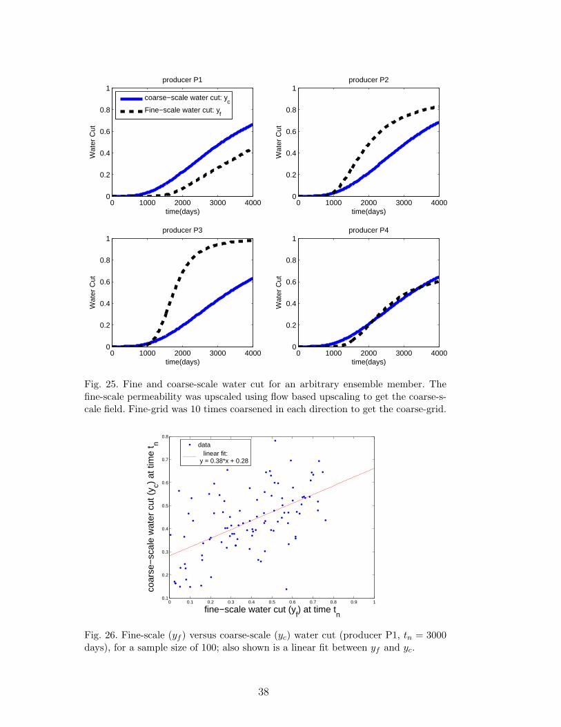
0 1000 2000 3000 40000
0.2
0.4
0.6
0.8
1producer P1
time(days)
Wat
er C
ut
0 1000 2000 3000 40000
0.2
0.4
0.6
0.8
1producer P2
time(days)
Wat
er C
ut
0 1000 2000 3000 40000
0.2
0.4
0.6
0.8
1producer P3
time(days)
Wat
er C
ut
0 1000 2000 3000 40000
0.2
0.4
0.6
0.8
1producer P4
time(days)
Wat
er C
ut
coarse−scale water cut: yc
Fine−scale water cut: yf
Fig. 25. Fine and coarse-scale water cut for an arbitrary ensemble member. Thefine-scale permeability was upscaled using flow based upscaling to get the coarse-s-cale field. Fine-grid was 10 times coarsened in each direction to get the coarse-grid.
0 0.1 0.2 0.3 0.4 0.5 0.6 0.7 0.8 0.9 10.1
0.2
0.3
0.4
0.5
0.6
0.7
0.8
fine−scale water cut (yf) at time t
n
coar
se−
scal
e w
ater
cut
(y c)
at ti
me
t n
data linear fit: y = 0.38*x + 0.28
Fig. 26. Fine-scale (yf ) versus coarse-scale (yc) water cut (producer P1, tn = 3000days), for a sample size of 100; also shown is a linear fit between yf and yc.
38
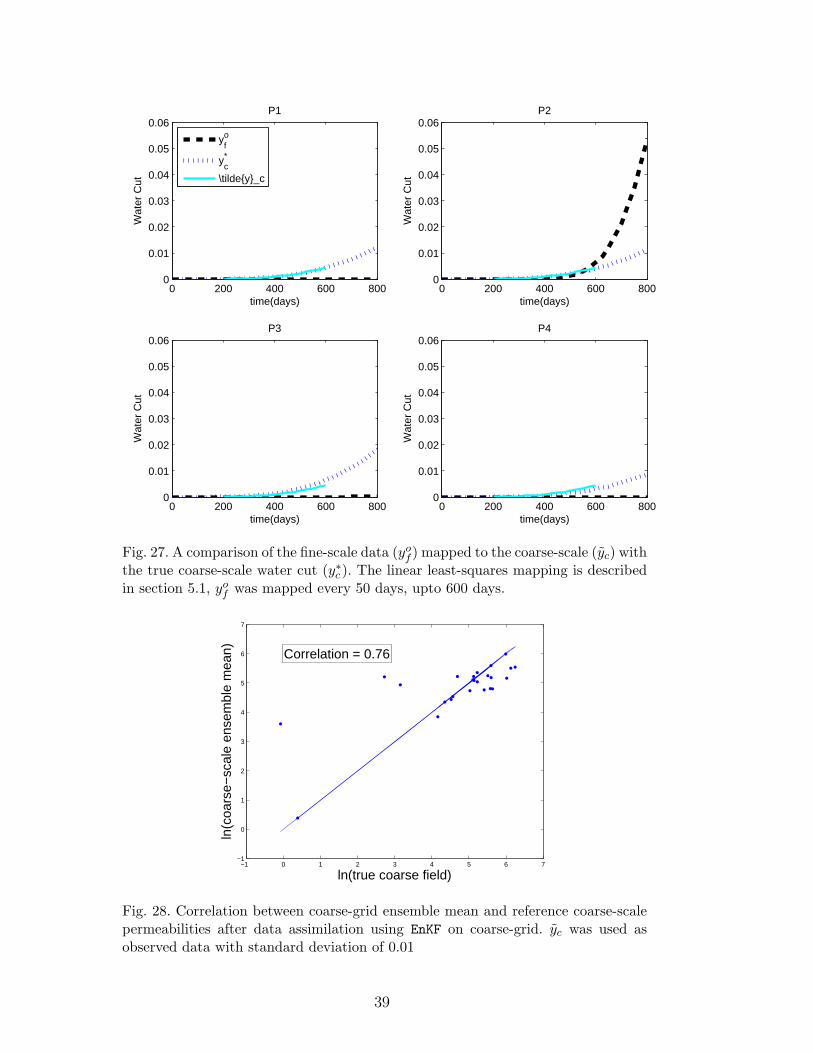
0 200 400 600 8000
0.01
0.02
0.03
0.04
0.05
0.06P1
time(days)
Wat
er C
ut
0 200 400 600 8000
0.01
0.02
0.03
0.04
0.05
0.06P2
time(days)
Wat
er C
ut
0 200 400 600 8000
0.01
0.02
0.03
0.04
0.05
0.06P3
time(days)
Wat
er C
ut
0 200 400 600 8000
0.01
0.02
0.03
0.04
0.05
0.06P4
time(days)
Wat
er C
ut
yof
y*c
\tildey_c
Fig. 27. A comparison of the fine-scale data (yof ) mapped to the coarse-scale (yc) with
the true coarse-scale water cut (y∗c ). The linear least-squares mapping is describedin section 5.1, yo
f was mapped every 50 days, upto 600 days.
−1 0 1 2 3 4 5 6 7−1
0
1
2
3
4
5
6
7
ln(true coarse field)
ln(c
oars
e−sc
ale
ense
mbl
e m
ean) Correlation = 0.76
Fig. 28. Correlation between coarse-grid ensemble mean and reference coarse-scalepermeabilities after data assimilation using EnKF on coarse-grid. yc was used asobserved data with standard deviation of 0.01
39