Embed Size (px)
Citation preview

Cluster Analysis
Hal Whitehead
BIOL4062/5062

• What is cluster analysis?
• Non-hierarchical cluster analysis– K-means
• Hierarchical divisive cluster analysis
• Hierarchical agglomerative cluster analysis– Linkage: single, complete, average, …– Cophenetic correlation coefficient
• Additive trees
• Problems with cluster analyses

Cluster Analysis
“Classification”
Maximize within cluster homogeneity
(similar individuals within cluster)
“The Search for Discontinuities”Discontinuities: places to put divisions between clusters
4 5 6 7 81
2
3
4
5
?

Discontinuities:
Discontinuities generally present:
taxonomy
social organization
community ecology??

Types of cluster analysis:
• Uses: data, dissimilarity, similarity matrix
• Non-hierarchical– K-means
• Hierarchical– Hierarchical divisive (repeated K-means, network
methods)
– Hierarchical agglomerative• single linkage, average linkage, ...
• Additive trees

Non-hierarchical Clustering Techniques:K-Means
• Uses data matrix with Euclidean distances
• Maximizes between-cluster variance for given number of clusters– i.e. Choose clusters to maximize F-ratio in 1-
way MANOVA

K-Means
Works iteratively:1. Choose number of clusters
2. Assigns points to clustersRandomly or some other clustering technique
3. Moves each point to other clusters in turn--increase in between cluster variance?
4. Repeat step 3. until no improvement possible

K-means with three clusters
0.0 0.2 0.4 0.6 0.8 1.0X
0.0
0.2
0.4
0.6
0.8
1.0
Y
0.0 0.2 0.4 0.6 0.8 1.0X
0.0
0.2
0.4
0.6
0.8
1.0
Y
0.0 0.2 0.4 0.6 0.8 1.0X
0.0
0.2
0.4
0.6
0.8
1.0
Y
0.0 0.2 0.4 0.6 0.8 1.0X
0.0
0.2
0.4
0.6
0.8
1.0
Y
0.0 0.2 0.4 0.6 0.8 1.0X
0.0
0.2
0.4
0.6
0.8
1.0
Y
0.0 0.2 0.4 0.6 0.8 1.0X
0.0
0.2
0.4
0.6
0.8
1.0
Y
0.0 0.2 0.4 0.6 0.8 1.0X
0.0
0.2
0.4
0.6
0.8
1.0
Y

K-means with three clusters
Variable Between SS df Within SS df F-ratio
X 0.536 2 0.007 7 256.163
Y 0.541 2 0.050 7 37.566
** TOTAL ** 1.078 4 0.058 14
0.0 0.2 0.4 0.6 0.8 1.0X
0.0
0.2
0.4
0.6
0.8
1.0
Y

K-means with three clusters
Cluster 1 of 3 contains 4 cases
Members Statistics
Case Distance | Variable Minimum Mean Maximum St.Dev.
Case 1 0.02 | X 0.41 0.45 0.49 0.04
Case 2 0.11 | Y 0.03 0.19 0.27 0.11
Case 3 0.06 |
Case 4 0.05 |
Cluster 2 of 3 contains 4 cases
Members Statistics
Case Distance | Variable Minimum Mean Maximum St.Dev.
Case 7 0.06 | X 0.11 0.15 0.19 0.03
Case 8 0.03 | Y 0.61 0.70 0.77 0.07
Case 9 0.02 |
Case 10 0.06 |
Cluster 3 of 3 contains 2 cases
Members Statistics
Case Distance | Variable Minimum Mean Maximum St.Dev.
Case 5 0.01 | X 0.77 0.77 0.78 0.01
Case 6 0.01 | Y 0.33 0.35 0.36 0.02
0.0 0.2 0.4 0.6 0.8 1.0X
0.0
0.2
0.4
0.6
0.8
1.0
Y

Disadvantages of K-means
• Reaches optimum, but not necessarily global
• Must choose number of clusters before analysis– How many clusters?

Example: Sperm whale codas
Patterned series of clicks:
| | | | |ic1 ic2 ic3 ic4
For 5-click codas: 681 x 4 data set

5-click codas:
| | | | |ic1 ic2 ic3 ic4
0.0 0.1 0.2 0.3 0.4 0.5 0.6ic1
0.1
0.2
0.3
0.4
0.5
0.6
0.7
ic4
-6 -2 2 61st Principal Component
-7
-3
1
5
2nd
Prin
cipa
l Com
pone
nt
93% of variance in 2 PC’s

5-click codas:K-means with 10 clusters
-6 -2 2 61st Principal Component
-7
-3
1
5
2nd
Prin
cipa
l Com
pone
nt
0.0 0.1 0.2 0.3 0.4 0.5 0.6ic1
0.1
0.2
0.3
0.4
0.5
0.6
0.7
ic4

Hierarchical Cluster Analysis
• Usually represented by:– Dendrogram or tree-diagram
Cluster Tree
0.0 0.1 0.2 0.3Distances
Case 1
Case 2
Case 3
Case 4
Case 5
Case 6
Case 7
Case 8
Case 9
Case 10

Hierarchical Cluster Analysis
• Hierarchical Divisive Cluster Analysis
• Hierarchical Agglomerative Cluster Analysis

Hierarchical Divisive Cluster Analysis
• Starts with all units in one cluster, successively splits them– Successive use of K-Means, or some other divisive
technique, with n=2– Either: Each time use the cluster with the greatest
sum of squared distances– Or: Split each cluster each time.
• Hierarchical divisive are good techniques, but rarely used, outside network analysis
0.70.60.50.40.30.20.1
1
14
15
4
5
11
9
19
2
12
20
Association index

Hierarchical Agglomerative Cluster Analysis
• Start with each individual units occupying its own cluster
• The clusters are then gradually merged until just one is left
• The most common cluster analyses
0.7 0.6 0.5 0.4 0.3 0.2 0.1
1
14
15
4
5
11
9
19
2
12
20
Association index

Hierarchical Agglomerative Cluster Analysis
Works on dissimilarity matrix or negative similarity matrixmay be Euclidean, Penrose, … distances
At each step:1. There is a symmetric matrix of dissimilarities between clusters 2. The two clusters with least dissimilarity are merged3. The dissimilarity between the new (merged) cluster and all
others is calculated
Different techniques do step 3. in different ways:

Hierarchical Agglomerative Cluster Analysis
A B C D E
A 0 . . . .
B 0.35 0 . . .
C 0.45 0.67 0 . .
D 0.11 0.45 0.57 0 .
E 0.22 0.56 0.78 0.19 0
AD B C E
AD 0 . . .
B ? 0 . .
C ? 0.67 0 .
E ? 0.56 0.78 0
First link A and D How to calculate new disimmilarities?

Hierarchical Agglomerative Cluster AnalysisSingle Linkage
A B C D E
A 0 . . . .
B 0.35 0 . . .
C 0.45 0.67 0 . .
D 0.11 0.45 0.57 0 .
E 0.22 0.56 0.78 0.19 0
AD B C E
AD 0 . . .
B 0.35 0 . .
C ? 0.67 0 .
E ? 0.56 0.78 0
d(AD,B)=Min{d(A,B), d(D,B)}

Hierarchical Agglomerative Cluster AnalysisComplete Linkage
A B C D E
A 0 . . . .
B 0.35 0 . . .
C 0.45 0.67 0 . .
D 0.11 0.45 0.57 0 .
E 0.22 0.56 0.78 0.19 0
AD B C E
AD 0 . . .
B 0.45 0 . .
C ? 0.67 0 .
E ? 0.56 0.78 0
d(AD,B)=Max{d(A,B), d(D,B)}

Hierarchical Agglomerative Cluster AnalysisAverage Linkage
A B C D E
A 0 . . . .
B 0.35 0 . . .
C 0.45 0.67 0 . .
D 0.11 0.45 0.57 0 .
E 0.22 0.56 0.78 0.19 0
AD B C E
AD 0 . . .
B 0.40 0 . .
C ? 0.67 0 .
E ? 0.56 0.78 0
d(AD,B)=Mean{d(A,B), d(D,B)}

Hierarchical Agglomerative Cluster AnalysisCentroid Clustering
(uses data matrix, or true distance matrix)V1 V2 V3
A 0.11 0.75 0.33
B 0.35 0.99 0.41
C 0.45 0.67 0.22
D 0.11 0.71 0.37
E 0.22 0.56 0.78
F 0.13 0.14 0.55
G 0.55 0.90 0.21
V1(AD)=Mean{V1(A),V1(D)}
V1 V2 V3
AD 0.11 0.73 0.35
B 0.35 0.99 0.41
C 0.45 0.67 0.22
E 0.22 0.56 0.78
F 0.13 0.14 0.55
G 0.55 0.90 0.21

Hierarchical Agglomerative Cluster AnalysisWard’s Method
• Minimizes within-cluster sum-of squares
• Similar to centroid clustering

0.7 0.6 0.5 0.4 0.3 0.2 0.1
1
14
15
4
5
11
9
19
2
12
20
Association index
Average Linkage
1 1.00
2 0.00 1.00
4 0.53 0.00 1.00
5 0.18 0.05 0.00 1.00
9 0.22 0.09 0.13 0.25 1.00
11 0.36 0.00 0.17 0.40 0.33 1.00
12 0.00 0.37 0.18 0.00 0.13 0.00 1.00
14 0.74 0.00 0.30 0.20 0.23 0.17 0.00 1.00
15 0.53 0.00 0.30 0.00 0.36 0.00 0.26 0.56 1.00
19 0.00 0.00 0.17 0.21 0.43 0.32 0.29 0.09 0.09 1.00
20 0.04 0.00 0.17 0.00 0.14 0.10 0.35 0.00 0.18 0.25 1.00
1 2 4 5 9 11 12 14 15 19 20

0.75 0.7 0.65 0.6 0.55 0.5 0.45 0.4 0.35 0.3
1
14
15
4
5
11
9
19
2
12
20
Association index
Single Linkage
0.7 0.6 0.5 0.4 0.3 0.2 0.1
1
14
15
4
5
11
9
19
2
12
20
Association index
Average Linkage
0.7 0.6 0.5 0.4 0.3 0.2 0.1 0
1
14
15
4
2
12
5
11
9
19
20
Association index
Complete Linkage
0.8 0.7 0.6 0.5 0.4 0.3 0.2 0.1 0
1
14
15
4
2
12
20
5
11
9
19
Association index
Ward's

Hierarchical Agglomerative Clustering Techniques
• Single Linkage– Produces “straggly” clusters– Not recommended if much experimental error– Used in taxonomy– Invariant to transformations
• Complete Linkage– Produces “tight” clusters– Not recommended if much experimental error– Invariant to transformations
• Average Linkage, Centroid, Ward’s– Most likely to mimic input clusters– Not invariant to transformations in dissimilarity measure

Cophenetic Correlation Coefficient CCC
• Correlation between original disimilarity matrix and dissimilarity inferred from cluster analysis
• CCC >~ 0.8 indicate a good match
• CCC <~ 0.8, dendrogram not a good representation– probably should not be displayed
• Use CCC to choose best linkage method (highest coefficient)
1 1.00
2 0.00 1.00
4 0.53 0.00 1.00
5 0.18 0.05 0.00 1.00
9 0.22 0.09 0.13 0.25 1.00
11 0.36 0.00 0.17 0.40 0.33 1.00
12 0.00 0.37 0.18 0.00 0.13 0.00 1.00
14 0.74 0.00 0.30 0.20 0.23 0.17 0.00 1.00
15 0.53 0.00 0.30 0.00 0.36 0.00 0.26 0.56 1.00
19 0.00 0.00 0.17 0.21 0.43 0.32 0.29 0.09 0.09 1.00
20 0.04 0.00 0.17 0.00 0.14 0.10 0.35 0.00 0.18 0.25 1.00
1 2 4 5 9 11 12 14 15 19 20
0.7 0.6 0.5 0.4 0.3 0.2 0.1
1
14
15
4
5
11
9
19
2
12
20
Association index
Average Linkage

0.75 0.7 0.65 0.6 0.55 0.5 0.45 0.4 0.35 0.3
1
14
15
4
5
11
9
19
2
12
20
Association index
Single Linkage
0.7 0.6 0.5 0.4 0.3 0.2 0.1
1
14
15
4
5
11
9
19
2
12
20
Association index
Average Linkage
0.7 0.6 0.5 0.4 0.3 0.2 0.1 0
1
14
15
4
2
12
5
11
9
19
20
Association index
Complete Linkage
0.8 0.7 0.6 0.5 0.4 0.3 0.2 0.1 0
1
14
15
4
2
12
20
5
11
9
19
Association index
Ward's
CCC=0.83
CCC=0.75
CCC=0.77
CCC=0.80
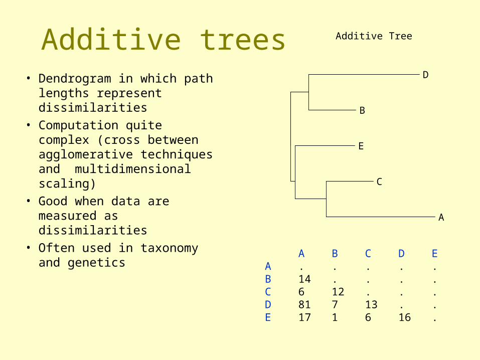
Additive trees• Dendrogram in which path
lengths represent dissimilarities
• Computation quite complex (cross between agglomerative techniques and multidimensional scaling)
• Good when data are measured as dissimilarities
• Often used in taxonomy and genetics
Additive Tree
A
B
C
D
E
A B C D EA . . . . .B 14 . . . .C 6 12 . . .D 81 7 13 . .E 17 1 6 16 .
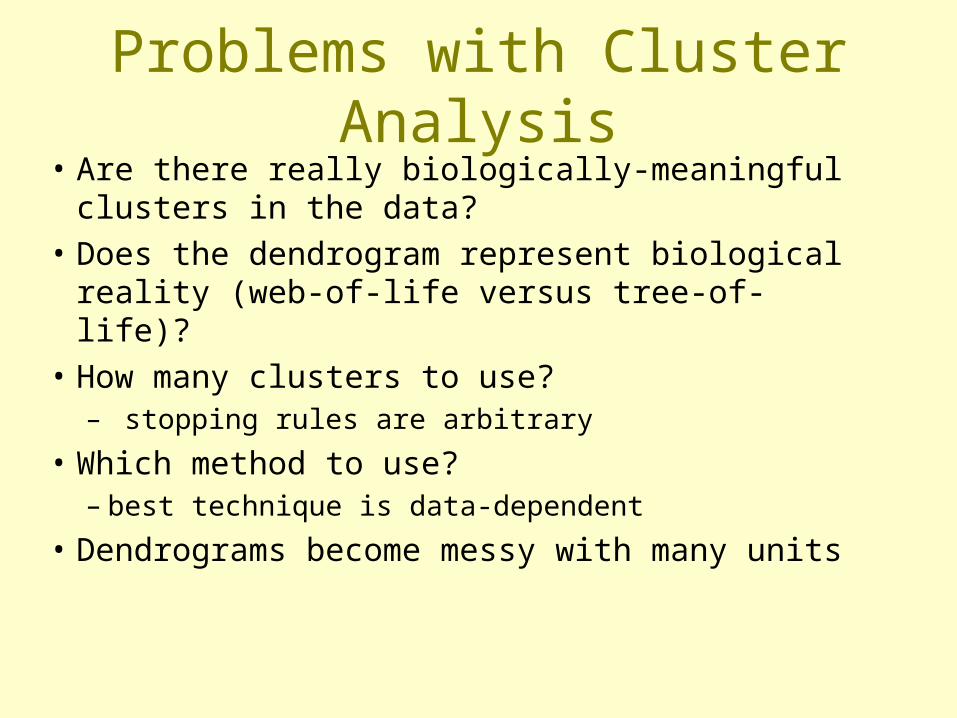
Problems with Cluster Analysis• Are there really biologically-meaningful clusters in
the data?• Does the dendrogram represent biological reality
(web-of-life versus tree-of-life)?• How many clusters to use?
– stopping rules are arbitrary
• Which method to use?– best technique is data-dependent
• Dendrograms become messy with many units

10.90.80.70.60.50.40.30.20.1 0
9179221367740757149316422515316539501501151215131515120613824103313111461019147054123956480133211161181426413170303115722246114351202252102222715980413642811141130711511181418371241431040114211431144832952961114910091025102010421045171081267409466106410752979861835787916818115731332515940644076451024727315231614157450250421394313489290509518165583051015088531563903991628829191271311132561931712121219122012685076747232353806512429591248134413451966213121441930165167186269649224623092310
Association index
Social Structure of 160 northern bottlenose whales

Clustering TechniquesType Technique Use
Non-hierarchical K-Means Dividing data sets
Hierarchical divisive Repeated K-means Good technique on
small data sets
Network methods...
Hierarchical agglomerative
Single linkage Taxonomy
Complete linkage Tighter Clusters
Average linkage,
Centroid, Ward’s Usually Preferred
Hierarchical Additive trees Excellent for displaying dissimilarity; taxonomy, genetics