Cluster algebras from surfaces - UCONNschiffler/LNCIMPA.pdf · 2.3 Cluster algebras from surfaces ... polynomials in the variables y 1 ... Let Xbe the set of all cluster variables

Cluster algebras from surfacesLecture notes for the CIMPA School

Mar del Plata, March 2016

Ralf SchifflerUniversity of Connecticut

2

Contents

0 Introduction 5

1 Cluster algebras 71.1 Ground ring ZP . . . . . . . . . . . . . . . . . . . . . . . . . . 71.2 Seeds and mutations . . . . . . . . . . . . . . . . . . . . . . . 81.3 Definition . . . . . . . . . . . . . . . . . . . . . . . . . . . . . 111.4 Example 1→ 2 . . . . . . . . . . . . . . . . . . . . . . . . . . 111.5 Example . . . . . . . . . . . . . . . . . . . . . . . . . . . . . 121.6 Laurent phenomenon and positivity . . . . . . . . . . . . . . . 131.7 Classifications . . . . . . . . . . . . . . . . . . . . . . . . . . . 14

2 Cluster algebras of surface type 172.1 Marked surfaces . . . . . . . . . . . . . . . . . . . . . . . . . . 172.2 Arcs and triangulations . . . . . . . . . . . . . . . . . . . . . . 182.3 Cluster algebras from surfaces . . . . . . . . . . . . . . . . . . 21

3 Snake graphs and expansion formulas 233.1 Snake graphs . . . . . . . . . . . . . . . . . . . . . . . . . . . 233.2 Band graphs . . . . . . . . . . . . . . . . . . . . . . . . . . . . 253.3 From snake graphs to surfaces . . . . . . . . . . . . . . . . . . 263.4 Labeled snake graphs from surfaces . . . . . . . . . . . . . . . 273.5 Perfect matchings, height and weight . . . . . . . . . . . . . . 283.6 Expansion formula . . . . . . . . . . . . . . . . . . . . . . . . 293.7 Examples . . . . . . . . . . . . . . . . . . . . . . . . . . . . . 30

4 Bases for the cluster algebra 334.1 Skein relations . . . . . . . . . . . . . . . . . . . . . . . . . . . 344.2 Definition of the bases B◦ and B. . . . . . . . . . . . . . . . . 36

3

4 CONTENTS

5 Appendix 415.1 Tagged arcs . . . . . . . . . . . . . . . . . . . . . . . . . . . . 415.2 Self-folded triangles . . . . . . . . . . . . . . . . . . . . . . . . 435.3 Expansion formula for singly-notched arcs . . . . . . . . . . . 445.4 Expansion formula for doubly-notched arcs . . . . . . . . . . . 455.5 Example for a singly-notched arc . . . . . . . . . . . . . . . . 465.6 Example for a doubly-notched arc . . . . . . . . . . . . . . . . 48

Chapter 0

Introduction

Cluster algebras were introduced by Fomin and Zelevinsky [FZ1] in 2002.Their original motivation was coming from canonical bases in Lie Theory.Today cluster algebras are connected to various fields of mathematics, in-cluding

• Combinatorics (polyhedra, frieze patterns, green sequences, snake graphs,T-paths, dimer models, triangulations of surfaces)

• Representation theory of finite dimensional algebras (cluster categories,cluster-tilted algebras, preprojective algebras, tilting theory, 2-Calbi-Yau categories, invariant theory)

• Poisson geometry and algebraic geometry (cluster varieties, Grassman-nians, stability conditions, scattering diagrams, Poisson structures onSL(n))

• Teichmuller theory (lambda-lengths, Penner coordinates, cluster vari-eties)

• Knot theory (Chern-Simons invariants, volume conjecture, Legendrianknots)

• Dynamical systems (frieze patterns, pentagram map, T-systems, sine-Gordon Y-systems)

• Mathematical Physics (statistical mechanics, Donaldson-Thomas in-variants, quantum dilogarithm identities, BPS particles)

5

6 CHAPTER 0. INTRODUCTION

Furthermore, because of an intensive research over the last 15 years, thesubject of cluster algebras itself has grown into an independent theory.

In this minicourse, we will focus on cluster algebras from surfaces, aspecial class of cluster algebras. The first chapter is a short introductionto cluster algebras, and chapters two, three and four are devoted to clusteralgebras from surfaces, especially to the expansion formulas for the clustervariables and the construction of canonical bases in terms of snake and bandgraphs. 1

1The author is supported by NSF CAREER grant DMS-1254567 and by the Universityof Connecticut.

Chapter 1

Cluster algebras

The definition of cluster algebras is elementary, but quite complicated. Wedescribe it in this first section. Since these notes are aiming for cluster alge-bras from surfaces, we do not present the most general definition of clusteralgebras, but restrict ourselves to so-called skew-symmetric cluster algebraswith principal coefficients. For the general definition and further details werefer to [FZ4].

1.1 Ground ring ZPTo define a cluster algebra A we must first fix its ground ring.

Let (P, ·) be a free abelian group (written multiplicatively) on variablesy1, . . . , yn and define an addition ⊕ in P by∏

j

yajj ⊕

∏j

ybjj =

∏j

ymin(aj ,bj)j . (1.1)

For example y21y−32 y3 ⊕ 1 = y−3

2 . Then (P,⊕, ·) is a semifield1, and is calledtropical semifield.

Let ZP denote the group ring of P. Then ZP is the ring of Laurentpolynomials in the variables y1, . . . , yn. The ring ZP will be the ground ringfor the cluster algebra.

1This means that ⊕ is commutative, associative and distributive with respect to themultiplication in P.

7

8 CHAPTER 1. CLUSTER ALGEBRAS

Remark 1.1 If this is the first time you see cluster algebras, then you mayconsider the special case where P = 1, and ZP = Z is just the ring of integers.In this case, we say the cluster algebra has trivial coefficients.

Let QP denote the field of fractions of ZP and let F = QP(x1, . . . , xn) bethe field of rational functions in n variables and coefficients in QP.

Remark 1.2 In the case of trivial coefficients, we have QP = Q.

1.2 Seeds and mutations

The cluster algebra is determined by the choice of an initial seed (x,y, Q),which consists of the following data.

• Q is a quiver without loops ◦ ee and 2-cycles ◦ // ◦oo , and with nvertices;

• y = (y1, . . . , yn) is the n-tuple of generators of P, called initial coeffi-cient tuple;

• x = (x1, . . . , xn) is the n-tuple of variables of F , called initial cluster.

The triple (x,y, Q) is called the initial seed of the cluster algebra A =A(x,y, Q).

The cluster algebra is the ZP-subalgebra of F generated by so-calledcluster variables, and these cluster variables are constructed from the initialseed by a recursive method called mutation. A mutation transforms a seed(x,y, Q) into a new seed (x′,y′, Q′). Given any seed there are n differentmutations µ1, . . . , µn, one for each vertex of the quiver, or equivalently, onefor each cluster variable in the cluster.

The seed mutation µk in direction k transforms (x,y, Q) into the seedµk(x,y, Q) = (x′,y′, Q′) defined as follows:

• x′ is obtained from x by replacing one cluster variable by a new one,x′ = x\{xk}∪{x′k}, and x′k is defined by the following exchange relation

xkx′k =

1

yk ⊕ 1

(yk∏i→k

xi +∏i←k

xi

)(1.2)

where the first product runs over all arrows in Q that end in k and thesecond product runs over all arrows that start in k.

1.2. SEEDS AND MUTATIONS 9

• y′ = (y′1, . . . , y′n) is a new coefficient n-uple, where

y′j =

y−1k if j = k;

yj∏k→j

yk(yk ⊕ 1)−1∏k←j

(yk ⊕ 1) if j 6= k.

Note that one of the two products is always trivial, hence equal to 1,since Q has no oriented 2-cycles. Also note that y′ depends only on yand Q.

• The quiver Q′ is obtained from Q in three steps:

1. for every path i→ k → j add one arrow i→ j,

2. reverse all arrows at k,

3. delete 2-cycles.

See Figure 1.1 for three examples of quiver mutations.

Lemma 1.3 Mutations are involutions, that is, µkµk(x,y, Q) = (x,y, Q).

Note that Q′ only depends on Q, that y′ depends on y and Q, and thatx′ depends on the whole seed (x,y, Q).

It is convenient to picture the mutation procedure in the so-called ex-change graph. The vertices of this graph are the seeds of the cluster algebraand the edges are the mutations. Since we can always mutate in n directions,each vertex in the exchange graph has exactly n neighbors. See Figure 1.2 foran example with n = 3. The initial seed is one of the vertices in this graph.Applying the first n mutations to this seed, will producet the n neighborsof this vertex in the graph, each of which contains exactly one new clustervariable. So at this stage we have 2n cluster variables. Now we can continuemutating these new seeds, and at every step we construct a “new” clustervariable. It may happen, that we obtain a seed that has already appearedpreviously in this process. In that case we identify the two correspondingvertices in the n-regular graph, and the actual exchange graph is a quotientof the graph in Figure 1.2. Such a repetition may happen but it does nothave to, and in general the number of seeds is infinite. The whole pattern isdetermined by the initial seed.


1 // 2 // 3µ2←→ 1

��2oo 3oo

2

��

1 //// 3

^^=======

µ2←→ 2

��=======

1

@@��// 3

5

2

^^=======

^^=======

��4oo

oooo

1 //// 3

^^=======

µ2←→ 5

��=======

��=======

2

��=======////// 4

ssssssssss

ss

cccccc1

@@��// 3

PPPP

Figure 1.1: Examples of quiver mutations

• •

• •

•~~~~

•@@@@ ~~~~

•@@@@

•~~~~ @@@@

• •

Figure 1.2: A 3-regular graph

1.3. DEFINITION 11

1.3 Definition

Let X be the set of all cluster variables obtained by mutation from (x,y, Q).The cluster algebra A = A(x,y, Q) is the ZP-subalgebra of F generated byX .

By definition, the elements of A are polynomials in X with coefficientsin ZP, so A ⊂ ZP[X ]. On the other hand, A ⊂ F , so the elements of A arealso rational functions in x1, . . . , xn with coefficients in QP.

Remark 1.4 Fomin and Zelevinsky define cluster algebras in a more generalsetting using skew-symmetrizable matrices instead of quivers. The quiver def-inition corresponds to the special case where the matrices are skew-symmetric.

1.4 Example 1→ 2

Let (x,y, Q) = ((x1, x2), (1, 1), 1→ 2).Since the coefficients in this example are trivial, the coefficients in any

seed will be {1, 1}. We therefore omit them in the computation below. Startwith the initial seed.

(x1, x2), 1→ 2

Apply mutation µ1. (x2 + 1

x1

, x2

), 1← 2


x1

,x2 + 1 + x1

x1x2

), 1→ 2

Apply mutation µ1. Let us do this step in detail. We get

x2+1+x1x1x2

+ 1x2+1x1

=(x2 + 1 + x1 + x1x2)x1

x1x2(x2 + 1)=

(x2 + 1)(x1 + 1)

x2(x2 + 1)=x1 + 1

x2

.

Note that the denominator is a monomial. Thus the new seed is(x1 + 1

x2

,x2 + 1 + x1

x1x2

), 1← 2



x2

, x1

), 1→ 2

Apply mutation µ1.(x2, x1), 1← 2

Continuing the process from here will not yield new cluster variables. Thusin this case, there are exactly 5 cluster variables

x1, x2,x2 + 1

x1

,x2 + 1 + x1

x1x2

,x1 + 1

x2

.

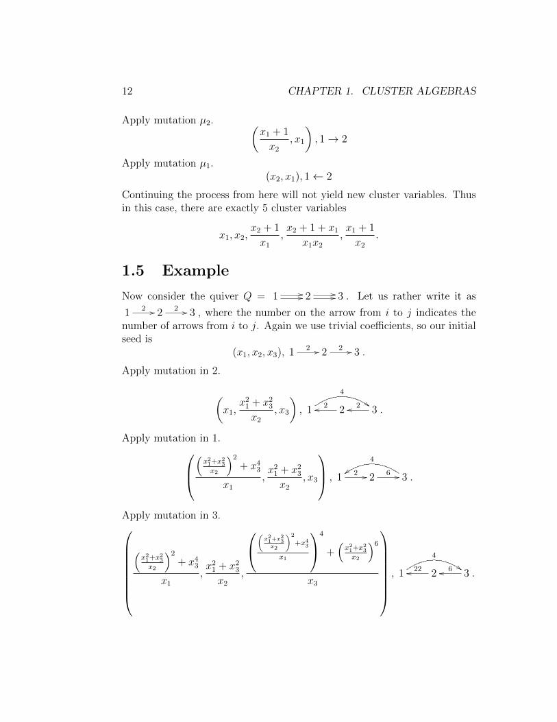
1.5 Example

Now consider the quiver Q = 1 //// 2 //// 3 . Let us rather write it as

1 2 // 2 2 // 3 , where the number on the arrow from i to j indicates thenumber of arrows from i to j. Again we use trivial coefficients, so our initialseed is

(x1, x2, x3), 1 2 // 2 2 // 3 .

Apply mutation in 2.

(x1,

x21 + x2

3

x2

, x3

), 1

4

$$22oo 32oo .

Apply mutation in 1.(x21+x23x2

)2

+ x43

x1

,x2

1 + x23

x2

, x3

, 1 2 // 2 6 // 3

4

zz.

Apply mutation in 3.(x21+x23x2

)2

+ x43

x1

,x2

1 + x23

x2

,

(x21+x

23

x2

)2

+x43

x1

4

+(x21+x23x2

)6

x3

, 1 oo 22 2 oo 6 3

$$4

.

1.6. LAURENT PHENOMENON AND POSITIVITY 13

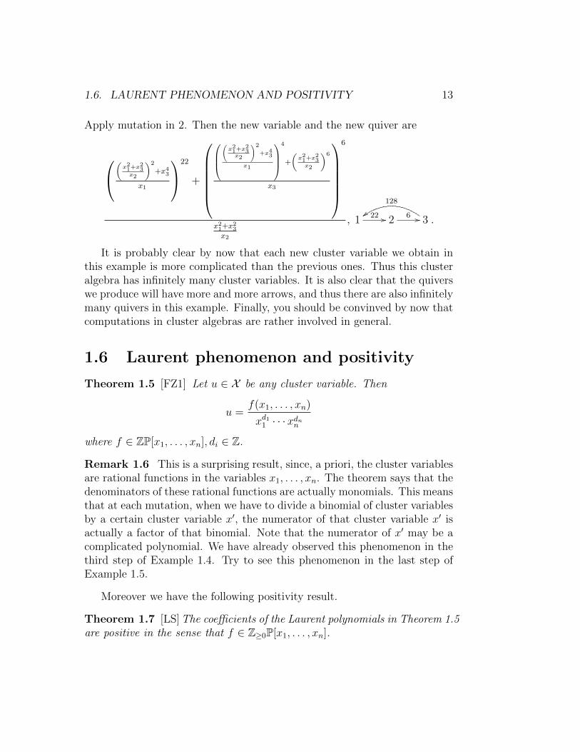
Apply mutation in 2. Then the new variable and the new quiver are

(x21+x

23

x2

)2

+x43

x1

22

+

(x21+x

23

x2

)2

+x43

x1

4

+

(x21+x

23

x2

)6

x3

6

x21+x23x2

, 1 22 // 2 6 // 3

128

zz.

It is probably clear by now that each new cluster variable we obtain inthis example is more complicated than the previous ones. Thus this clusteralgebra has infinitely many cluster variables. It is also clear that the quiverswe produce will have more and more arrows, and thus there are also infinitelymany quivers in this example. Finally, you should be convinved by now thatcomputations in cluster algebras are rather involved in general.

1.6 Laurent phenomenon and positivity

Theorem 1.5 [FZ1] Let u ∈ X be any cluster variable. Then

u =f(x1, . . . , xn)

xd11 · · ·xdnnwhere f ∈ ZP[x1, . . . , xn], di ∈ Z.

Remark 1.6 This is a surprising result, since, a priori, the cluster variablesare rational functions in the variables x1, . . . , xn. The theorem says that thedenominators of these rational functions are actually monomials. This meansthat at each mutation, when we have to divide a binomial of cluster variablesby a certain cluster variable x′, the numerator of that cluster variable x′ isactually a factor of that binomial. Note that the numerator of x′ may be acomplicated polynomial. We have already observed this phenomenon in thethird step of Example 1.4. Try to see this phenomenon in the last step ofExample 1.5.

Moreover we have the following positivity result.

Theorem 1.7 [LS] The coefficients of the Laurent polynomials in Theorem 1.5are positive in the sense that f ∈ Z≥0P[x1, . . . , xn].


Remark 1.8 This result is not obvious; and actually 13 years have passedbetween the proof of Theorem 1.5 and the proof of Theorem 1.7. Althoughthe binomial exchange relations only involve positive terms, one has to makesure that positivity is preserved when reducing the rational functions that oneobtains in the mutation procedure to the Laurent polynomials in the theorems.This is not true for arbitrary rational functions as the example x3+1

x+1= x2 −

x+ 1 shows.

1.7 Classifications

There are several special types of cluster algebras that have been studiedusing very different methods. We define these types here and show how theyoverlap.

We say that two quivers Q,Q′ are mutation equivalent, and write Q ∼ Q′,if there exists a finite sequence of muations transforming Q into Q′.

Definition 1.9 A cluster algebra A(x,y, Q) is said to be of

(a) finite type if the number of cluster variables is finite;

(b) finite mutation type if the number of quivers Q′ that are mutation equiv-alent to Q is finite;

(c) acyclic type if Q is mutation equivalent to a quiver without orientedcycles;

(d) surface type if Q is the adjacency quiver of a triangulation of a markedsurface (see Chapter 2).

The cluster algebra of Example 1.4 is of finite type, finite mutation type,acyclic type and surface type. On the other hand, the cluster algebra ofExample 1.5 is not of finite type, not of finite mutation type, not of surfacetype, but it is of acyclic type.

Fomin and Zelevinsky showed that the finite-type cluster algebras areclassified by the Dynkin diagrams. Since we are considering only clusteralgebras given by quivers, we only get the simply laced Dynkin diagrams.

Theorem 1.10 [FZ2] The cluster algebra A(x,y, Q) is of finite type if andonly if Q is mutation equivalent to a quiver of Dynkin type A,D or E.

1.7. CLASSIFICATIONS 15

acylcic finite mutation

finite

affine

E6,7,8

E6,7,8

E(1,1)6,7,8 X6,7

all but 11 areof surface type

Figure 1.3: Different types of cluster algebras of rank n ≥ 3

Finite mutation type is more general than finite type. The finite mutationtype classification is due to Felikson, Shapiro and Tumarkin.

Theorem 1.11 [FeShTu] The cluster algebra A(x,y, Q) is of finite mutationtype if and only if

• it is of surface type or

• n ≤ 2, or

• it is one of 11 exceptional types E6,E7,E8, E6, E7, E8,E(1,1)6 ,E(1,1)

7 ,E(1,1)8 ,

X6,X7.

The overlaps of the various classes of cluster algebras for n ≥ 3 areillustrated in Figure 1.3. The accylic and the mutation finite types have incommon the finite types A,D,E and the tame types corresponding to theextended Dynkin diagrams A, D, E. Other acyclic types are called wild. The11 exceptions in Theorem 1.11 are indicated by dots; 9 of them correspond toroot systems of certain E-types. The other 2 types X6,X7 had not appearedelsewhere before this classification.


Chapter 2

Cluster algebras of surface type

Building on work of Fock and Goncharov [FG1, FG2], and of Gekhtman, Shapiro

and Vainshtein [GSV], Fomin, Shapiro and Thurston [FST] associated a cluster

algebra to any bordered surface with marked points.

2.1 Marked surfaces

We fix the following notation.

• S is a connected oriented Riemann surface with (possibly empty) bound-ary ∂S.

• M ⊂ S is a finite set of marked points with at least one marked pointon each connected component of the boundary.

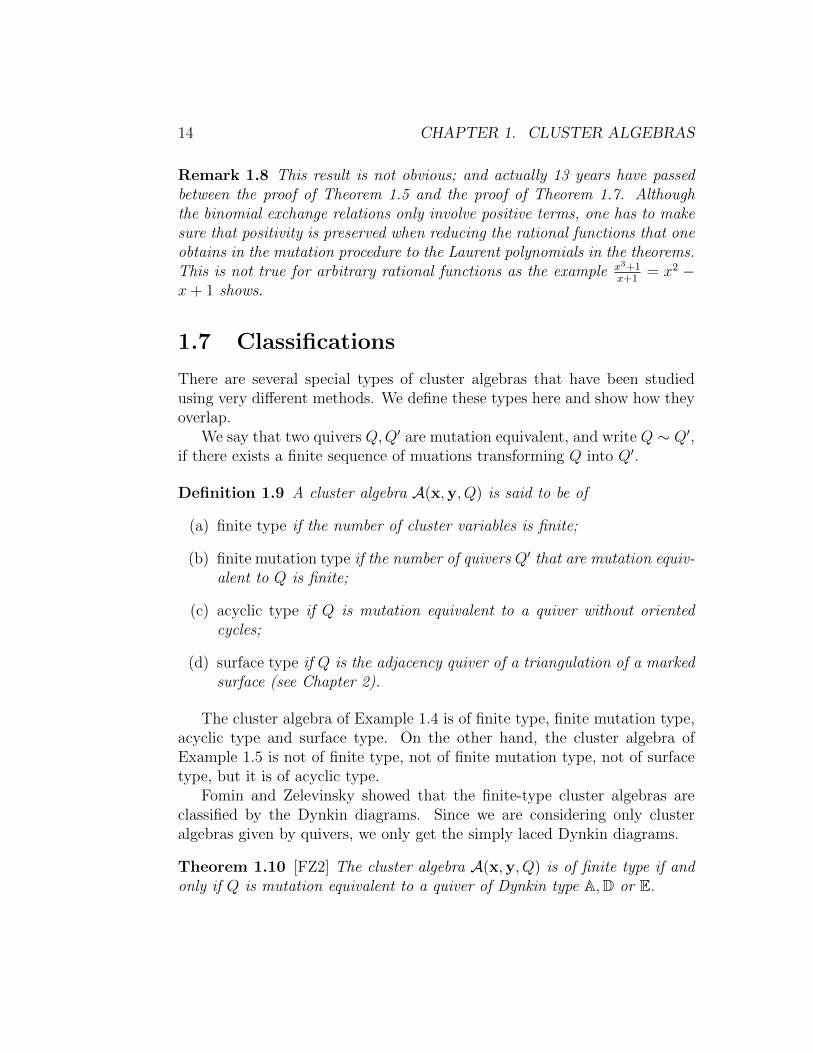
We will refer to the pair (S,M) simply as a surface. A surface is calledclosed if the boundary is empty. Marked points in the interior of S are calledpunctures. Examples are shown in Figure 2.1. For technical reasons, werequire that (S,M) is not a sphere with 1, 2 or 3 punctures; a monogon with0 or 1 puncture; or a bigon or triangle without punctures.

Remark 2.1 in Chapters 3 and 4, we will restrict to surfaces without punc-tures. The reason for this restriction in Chapter 3 is only for the sake ofsimplicity, but in Chapter 4 it is necessary. In the appendix, we explain howto modify the results in Chapter 3 in the presence of punctures.

17

18 CHAPTER 2. CLUSTER ALGEBRAS OF SURFACE TYPE

b=2

g=0

g=1

g=2

b=0 b=1

Figure 2.1: Examples of surfaces, g is the genus and b the number of boundarycomponents

2.2 Arcs and triangulations

An arc γ in (S,M) is a curve in S, considered up to isotopy1, such that

(a) the endpoints of γ are in M ;

(b) except for the endpoints, γ is disjoint from M and from ∂S,

(c) γ does not cut out an unpunctured monogon or an unpunctured bigon;

(d) γ does not cross itself, except that its endpoints may coincide.

A generalized arc is a curve which satisfies conditions (a),(b) and (c), butit can have selfcrossings. Curves that connect two marked points and lieentirely on the boundary of S without passing through a third marked pointare called boundary segments. By (c), boundary segments are not arcs. Aclosed loop is a closed curve in S which is disjoint from the boundary of S.

1A homotopy between two continuous maps f, g : X → Y is a continuous map h : [0, 1]×X → Y such that h(0, x) = f(x) and h(1, x) = g(x). An isotopy is a homotopy h suchthat for all t ∈ [0, 1] the map h(t,−) : X → h(t,X) is a homeomorphism. In particular anisotopy of curves cannot create selfcrossings.

2.2. ARCS AND TRIANGULATIONS 19

1 2

3 4

5

6

1 2

3 4

56

Figure 2.2: Two ideal triangulations of a punctured annulus related by aflip of the arc 6. The triangulation on the right hand side has a self-foldedtriangle.

For any two arcs γ, γ′ in S, define

e(γ, γ′) = min{number of crossings of α and α′ | α ' γ, α′ ' γ′},

where α and α′ range over all arcs isotopic to γ and γ′, respectively. We saythat arcs γ and γ′ are compatible if e(γ, γ′) = 0.

An ideal triangulation is a maximal collection of pairwise compatible arcs(together with all boundary segments). The arcs of a triangulation cut thesurface into ideal triangles. Triangles that have only two distinct sides arecalled self-folded triangles. Note that a self-folded triangle consists of a loop`, together with an arc r to an enclosed puncture which we call a radius.Examples of ideal triangulations are given in Figure 2.2 as well as in Figures3.5 and 3.6.

Lemma 2.2 The number of arcs in an ideal triangulation is exactly

n = 6g + 3b+ 3p+ c− 6,

where g is the genus of S, b is the number of boundary components, p is thenumber of punctures and c = |M | − p is the number of marked points on theboundary of S. The number n is called the rank of (S,M).

For the sake of completness, we include a proof of this fact, since it isusually omitted in the cited research papers.


Proof. Recall that the Euler characteristic of a surface S is given byχ(S) = f −e+v, where v is the number of vertices, e is the number of edges,and f is the number of faces in any triangulation of S. By induction on thegenus, one can show that for a closed surface χ(S) = 2 − 2g. Moreover, ifthe boundary of S has b connected components then

χ(S) = 2− 2g − b, (2.1)

since removing a disk from S can be thought of reducing the number of facesby one. Now consider a set of marked points M and a triangulation T . Thenthe number of vertices in T is |M | = c+ p. The number of edges in T is thenumber of arcs n plus the number of boundary segments c. Thus

e = c+ n and v = c+ p. (2.2)

We use induction on p. If p = 0, then each triangle has 3 distinct sides. Eachof the n arcs lies in precisely 2 triangles and each of the c boundary segmentslies in precisely 1 triangle. Therefore

3f = 2n+ c. (2.3)

Using equations (2.1)–(2.3) we get

2n+ c

3− c− n+ c = 2− 2g − b,

and the statement follows.

Now suppose that p > 0. Let T be a triangulation of (S,M), and let usadd a puncture x. Then we need to add 3 arcs to complete the triangulation.Indeed, the new puncture x lies in some triangle ∆ of the old triangulationT and connecting x with the three vertices of ∆ completes the triangulation.Thus adding a puncture increases n by 3. �

Ideal triangulations are connected to each other by sequences of flips.Each flip replaces a single arc γ in T by a unique new arc γ′ 6= γ such that

T ′ = (T \ {γ}) ∪ {γ′}

is a triangulation. See Figure 2.3.

2.3. CLUSTER ALGEBRAS FROM SURFACES 21

γ γ′flip γγ γ′flip γ

Figure 2.3: Two examples of flips

2.3 Cluster algebras from surfaces

We are now ready to define the cluster algebra associated to the surface.For that purpose, we choose an ideal triangulation T = {τ1, τ2, . . . , τn} andthen define a quiver QT without loops or 2-cycles as follows. The verticesof QT are in bijection with the arcs of T , and we denote the vertex of QT

corresponding to the arc τi simply by i. The arrows of QT are defined asfollows. For any triangle ∆ in T which is not self-folded, we add an arrowi→ j whenever

(a) τi and τj are sides of ∆ with τj following τi in the clockwise order;

(b) τj is a radius in a self-folded triangle enclosed by a loop τ`, and τi andτ` are sides of ∆ with τ` following τi in the clockwise order;

(c) τi is a radius in a self-folded triangle enclosed by a loop τ`, and τ` andτj are sides of ∆ with τj following τ` in the clockwise order;

Then we remove all 2-cycles.For example, the quiver corresponding to the triangulation on the right

of Figure 2.2 is

1

))SSSSSSSSSSS 3

))SSSSSSSSSSS

��2

55kkkkkkkkkkk 4

6

55kkkkkkkkkkk 5

iiSSSSSSSSSSS

55kkkkkkkkkkk

To define an initial seed, we associate an indeterminate xi to each τi ∈ Tand set the initial cluster xT = (x1, . . . , xn); and we set the initial coefficienttuple yT = (y1, . . . , yn) to be the vector of generators of P. Then the cluster


algebra A = A(xT ,yT , QT ) is called the cluster algebra associated to thesurface (S,M) with principal coefficients in T .

Fomin, Shapiro and Thurston showed that, up to a change of coefficients,the cluster algebra does not depend on the choice of the initial triangulationT . Moreover, they proved the following correspondence.

Theorem 2.3 [FST] There are bijections

{cluster variables of A} oo // {arcs of (S,M)}xγ γ

{clusters of A} oo // {triangulations of (S,M)}xT = {xγ1 , . . . , xγn} T = {γ1, . . . , γn}

Moreover, if γk is not the radius of a self-folded triangle in a triangulationT , then the mutation in k corresponds to the flip of the arc γk, that is, thecluster

µk(xT ) = (xT \ {xγk}) ∪ {x′γk}

corresponds to the triangulation

µγk(T ) = (T \ {γk}) ∪ {γ′k}.

Remark 2.4 For simplicity, we excluded the case where γk is the radius ofa self-folded triangle because then γk cannot be flipped. In [FST] the authorssolve this problem by introducing tagged arcs and tagged triangulations, re-placing the loop of a self-folded triangle by a second radius. In that setup thetheorem holds without any restrictions.

Remark 2.5 If β is a boundary segment, we set xβ = 1.

Chapter 3

Snake graphs and expansionformulas

Abstract snake graphs and band graphs were introduced and studied in [CS,CS2, CS3] motivated by the snake graphs and band graphs appearing inthe combinatorial formulas for cluster algebra elements in [Pr, MS, MSW,MSW2]. Throughout we fix the standard orthonormal basis of the plane.

3.1 Snake graphs

A tile G is a square in the plane whose sides are parallel or orthogonal tothe elements in the fixed basis. All tiles considered will have the same sidelength.

GWest East

North

South

We consider a tile G as a graph with four vertices and four edges in theobvious way. A snake graph G is a connected planar graph consisting of afinite sequence of tiles G1, G2, . . . , Gd, with d ≥ 1, such that for each i, thetiles Gi and Gi+1 share exactly one edge ei, and this edge is either the northedge of Gi and the south edge of Gi+1, or it is the east edge of Gi and thewest edge of Gi+1. An example of a snake graph with 8 tiles is given in Figure3.1.

23

24 CHAPTER 3. SNAKE GRAPHS AND EXPANSION FORMULAS

G1 G2

G3

G4 G5

G6 G7 G8

e2

e3

e4

e5

e6 e7

e1

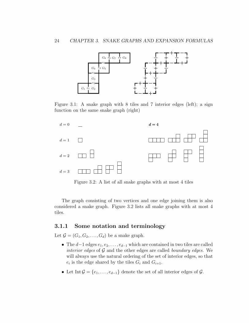
Figure 3.1: A snake graph with 8 tiles and 7 interior edges (left); a signfunction on the same snake graph (right)

d = 0

d = 1

d = 2

d = 3

d = 4d = 4

Figure 3.2: A list of all snake graphs with at most 4 tiles

The graph consisting of two vertices and one edge joining them is alsoconsidered a snake graph. Figure 3.2 lists all snake graphs with at most 4tiles.

3.1.1 Some notation and terminology

Let G = (G1, G2, . . . , Gd) be a snake graph.

• The d−1 edges e1, e2, . . . , ed−1 which are contained in two tiles are calledinterior edges of G and the other edges are called boundary edges. Wewill always use the natural ordering of the set of interior edges, so thatei is the edge shared by the tiles Gi and Gi+1.

• Let IntG = {e1, . . . , ed−1} denote the set of all interior edges of G.

3.2. BAND GRAPHS 25

• Let SWG, GNE denote the following sets.

SWG = { south edge of G1, west edge of G1 };

GNE = { north edge of Gd, east edge of Gd }.If G is a single edge, we let SWG = ∅ and GNE = ∅.

• We say that two snake graphs are isomorphic if they are isomorphic asgraphs.

3.1.2 Sign function

A sign function f on a snake graph G is a map

f : {edges of G} → {+,−},

such that on every tile in G• the north and the west edge have the same sign,

• the south and the east edge have the same sign

• the sign on the north edge is opposite to the sign on the south edge.

See Figure 3.1 for an example. Note that on every snake graph there areexactly two sign functions.

A snake graph is determined up to symmetry by its sequence of tilestogether with a sign function on the interior edges.

3.2 Band graphs

Band graphs are obtained from snake graphs by identifying a boundary edgeof the first tile with a boundary edge of the last tile, where both edges havethe same sign. We use the notation G◦ for general band graphs, indicatingtheir circular shape, and we also use the notation Gb if we know that theband graph is constructed by glueing a snake graph G along an edge b.

More precisely, to define a band graph G◦, we start with an abstractsnake graph G = (G1, G2, . . . , Gd) with d ≥ 1, and fix a sign function onG. Denote by x the southwest vertex of G1, let b ∈ SWG the south edge(respectively the west edge) of G1, and let y denote the other endpoint of b,see Figure 3.3. Let b′ be the unique edge in GNE that has the same sign asb, and let y′ be the northeast vertex of Gd and x′ the other endpoint of b′.


bx

yx′ y′b′

bx

y

x′ y′b′

b

b

b

b′b′

b′

xx

x

y = x′y

y

y′ y′y′

x′

x′

Figure 3.3: Examples of small band graphs; the two band graphs with 3 tilesare isomorphic.

Let Gb denote the graph obtained from G by identifying theedge b with the edge b′ and the vertex x with x′ and y with y′.The graph Gb is called a band graph or ouroborus1. Note thatnon-isomorphic snake graphs can give rise to isomorphic bandgraphs. See Figure 3.3 for examples.

The interior edges of the band graph Gb are by definition the interior edgesof G plus the glueing edge b = b′. A band graph is uniquely determined byits sequence of tiles G1, . . . , Gd together with its sign function on the interioredges (including the glueing edge).

In order to be able to formally take sums of band graphs we make thefollowing definition.

Definition 3.1 Let R denote the free abelian group generated by all isomor-phism classes of finite disjoint unions of snake graphs and band graphs. If Gis a snake graph, we also denote its class in R by G, and we say that G ∈ Ris a positive snake graph and that its inverse −G ∈ R is a negative snakegraph.

3.3 From snake graphs to surfaces

Given a snake graph G = (G1, G2, . . . , Gd), we can construct a triangulatedpolygon as follows.

• In each tile Gi add a diagonal τi from the north west corner to thesouth east corner.

• Tilt the snake graph such that each tile becomes a parallelogram con-sisting of two equilateral triangles.

1Ouroboros: a snake devouring its tail.

3.4. LABELED SNAKE GRAPHS FROM SURFACES 27

• Fold the snake graph along the interior edges e1, . . . , ed−1, and, at eachfolding, identify the two triangles on either side of the interior edge.

This produces a surface that is homeomorphic to a triangulated polygon withd+ 3 vertices whose set of boundary segments is precisely SWG ∪ IntG ∪GNEand whose triangulation is given by the diagonals τ1, . . . , τd.

Exercise 3.2 Cut out the following figure and perform the folding. Interioredges are black.

A labeled snake graph is a snake graph in which each edge and each tilecarries a label or weight. For example, for snake graphs from cluster algebrasof surface type, these labels are cluster variables.

3.4 Labeled snake graphs from surfaces

Now we want to go the other way and associate a snake graph to every arcin a triangulated surface.

Let T be an ideal triangulation of a surface (S,M) and let γ be an arcin (S,M) which is not in T . Choose an orientation on γ, let s ∈ M be itsstarting point, and let t ∈M be its endpoint. Denote by

s = p0, p1, p2, . . . , pd+1 = t

the points of intersection of γ and T in order. For j = 1, 2, . . . , d, let τij bethe arc of T containing pj, and let ∆j−1 and ∆j be the two ideal triangles in


∆10

∆9

∆0

∆1

∆2 ∆3

e1

e2 e3

e4

e9

τi1

e5 e6

e7 e8

∆4

∆5 ∆6

∆7 ∆8

τi2 τi3 τi4 τi5 τi6 τi7 τi8 τi9 τi10

γs t

Figure 3.4: The arc γ passing through d+ 1 triangles ∆0, . . . ,∆d

T on either side of τij . Then, for j = 1, . . . , d− 1, the arcs τij and τij+1form

two sides of the triangle ∆j in T and we define ej to be the third arc in thistriangle, see Figure 3.4.

Let Gj be the quadrilateral in T that contains τij as a diagonal. We willthink of Gj as a tile as in section 3.1, but now the edges of the tile are arcsin T and thus are labeled edges. We also think of the tile Gj itself beinglabeled by the diagonal τij .

Define a sign function f on the edges e1, . . . , ed by

f(ej) =

{+1 if ej lies on the right of γ when passing through ∆j

−1 otherwise.

The labeled snake graph Gγ = (G1, . . . , Gd) with tiles Gi and sign functionf is called the snake graph associated to the arc γ. Each edge e of Gγ is labeledby an arc τ(e) of the triangulation T . We define the weight x(e) of the edgee to be cluster variable associated to the arc τ(e). Thus x(e) = xτ(e).

Note that we can define a sign function f in the same way for a any closedloop ζ. In that case we define the band graph G◦ζ of ζ to be the band graphwith tiles Gi and sign function f .

3.5 Perfect matchings, height and weight

A perfect matching of a graph G is a subset P of the edges of G such thateach vertex of G is incident to exactly one edge of P . We define

MatchG = {perfect matchings of G}.

If G◦ = Gb is a band graph, we define MatchG◦ to be the set of all perfectmatchings P of the snake graph G such that P is a perfect matching of G◦.

3.6. EXPANSION FORMULA 29

Each snake graph G has precisely two perfect matchings P−, P+ that con-tain only boundary edges. We call P− the minimal matching and P+ themaximal matching of G. 2

P− P = (P− ∪ P ) \ (P− ∩ P ) denotes the symmetric difference of anarbitrary perfect matching P ∈ MatchG with the minimal matching P−.

Definition 3.3 Let P ∈ MatchG. The set P− P is the set of boundaryedges of a (possibly disconnected) subgraph GP of G, and GP is a union oftiles

GP =⋃i

Gi.

We define the height monomial of P by

y(P ) =∏

Gi a tile in GP

yi

Thus y(P ) is the product of all yi for which the tile Gi lies inside in P P−with multiplicities.

3.6 Expansion formula

Let T = {τ1, . . . , τn} be a triangulation of (S,M) and let A = A(xT ,yT , QT )be the cluster algebra with principal coefficients at T . Thus xT = (x1, . . . , xn),yT = (y1, . . . , yn) and P = Trop(y1, . . . , yn).

For simplicity, we assume here that there are no self-folded triangles inT . For the general case see the appendix.

Theorem 3.4 [MSW] Let γ be an arc not in the triangulation T . Then thecluster variable xγ is equal to

xγ =1

cross(γ)

∑P∈MatchGγ

x(P )y(P ),

where x(P ) =∏

e∈P x(e) is the weight of P , y(P ) is the height of P and

cross(γ) =∏d

j=1 xij .

2There is a choice involved here which of the two is P− and this will make a differencelater when we consider expansion formulas for cluster algebras with non-trivial coefficients.One can determine P− as follows. If a tile Gj has the same orientation as the surface Sthe P− contains the south and the north edges of Gj if they are boundary edges, and P−does not contain the east or the west edge of Gj .


Since this theorem gives us a direct formula for the cluster variables, itallows us to redefine the cluster algebra without using mutations as in thefollowing corollary.

Corollary 3.5 The cluster algebra A of the surface (S,M) with principalcoefficients in the triangulation T is the ZP subalgebra of F generated by all

1

cross(γ)

∑P∈MatchGγ

x(P )y(P ),

where γ runs over all arcs in (S,M).

3.7 Examples

In the example in Figure 3.5, we compute the snake graph Gγ of an arc γin a triangulated polygon. The arc γ crosses two arcs of the triangulation,hence the snake graph Gγ has two tiles. The graph Gγ admits exactly 3perfect matchings (drawn in red), and they form a linear poset in which P−is the unique minimal element and P+ is the unique maximal element. Thecorresponding monomials are listed in the rightmost column. Thus in thisexample we have

xγ =x1 y1y2 + x3 y1 + x2

x1x2

.

In the example in Figure 3.6, we compute the snake graph Gγ of an arcγ in a triangulated annulus. The arc γ crosses the triangulation three times,twice in the arc labeled 1 and once in the arc labeled 2. Hence the snakegraph Gγ has two tiles labeled 1 and one tile labeled 2. The graph Gγ admitsexactly 5 perfect matchings drawn in red in the poset. The correspondingmonomials are listed on the right of the poset. Thus in this example we have

xγ =x2

1 y21y2 + y2

1 + 2x22 y1 + x4

2

x21x2

.

3.7. EXAMPLES 31

1

32

γa

b

c

d

e

f x2

x3 y1

x1 y1y2

1 2

1 2

1 2

1

2

1

1

2

2

3

a

b

d

c

Gγ

Figure 3.5: An arc γ in a triangulated hexagon (left), it’s snake graph Gγ(center left) and its poset of perfect matchings (center right), and the cor-responding monomials (right). The edges labeled a,b,c,d,e,f are boundaryedges and their weights are one. The edges labeled 1,2,3 are arcs in the tri-angulation and their weights are the cluster variables x1, x2, x3, respectively.


21

b

a

γ

2

b 1

2

a

1

2

1

2

2

1b

a

1 12

1 12

1 12 1 12

1 12

1 1

1 1

2

x42

x22 y1 x2

2 y1

y21

x21 y

21y2

Gγ

Figure 3.6: An arc γ in a triangulated annulus (top left), it’s snake graphGγ (top right), the poset of perfect matchings of Gγ (bottom left), and thecorresponding monomials (bottom right). The edges labeled a,b are bound-ary edges and their weights are one. The edges labeled 1,2 are arcs in thetriangulation and their weights are the cluster variables x1, x2, respectively.

Chapter 4

Bases for the cluster algebra

We would like to have a unique way to write each element of the clusteralgebra as a sum of elements of a fixed basis. Recall the mutation exchangerelations (1.2) among the cluster variables

(yk ⊕ 1)xkx′k = yk

∏i→k

xi +∏i←k

xi.

This is an example of an element of the cluster algebra that can be writtenin two different ways. We would like a unique way. In this section, we presenttwo solutions to this problem for cluster algebras of surface type.

From now on let A = A(xT ,yT , QT ) be a cluster algebra arising froma surface (S,M) with principal coefficients at a fixed triangulation T , andassume that the surface has no punctures.1 Since the cluster algebra isgenerated by cluster variables, we need to understand (sums of) products ofcluster variables. Since cluster variables are in bijection with arcs, productsof cluster variables are in bijection with sets of arcs with multiplicities. Wecall a set of curves with multiplicities a multicurve.

Moreover, to each arc we have associated a snake graph which allows usto compute the cluster variable via the perfect matching formula of Theo-rem 3.4. Therefore a product of cluster variables can be computed by thesame perfect matching formula, replacing the single snake graph by a unionof snake graphs. We get the following diagram

1So far, restricting to the case without punctures has been for the sake of simplicity.But now we really need to make this restriction.

33

34 CHAPTER 4. BASES FOR THE CLUSTER ALGEBRA

product of cluster variables // multicurve

��Laurent expansion union of snake graphsoo

t∏i=1

(xγi)εi //

t⊔i=1

εi⊔j=1

{γi}

��

1cross(G)

∑P∈MatchG

x(P )y(P ) G =t⊔i=1

εi⊔j=1

Gγioo

4.1 Skein relations

The relations among the cluster variables can be expressed on the level ofarcs using smoothing operations [MW] and on the level of snake graphs asresolutions [CS, CS2, CS3].

Let γ1 and γ2 be two curves that cross at a point x. Then we define thesmoothing of {γ1, γ2} at x to be the pair of multicurves {γ3, γ4} and {γ5, γ6}obtained from {γ1, γ2} by replacing the crossing× in a small neighborhoodof x with the pair of segments _ (respectively ⊃⊂).

{γ1, γ2}smoothing at x // {γ3, γ4} , {γ5, γ6}

If γ is a curve with a selfcrossing at a point x, we also define the smoothingof γ at x to be the pair of curves γ34 and γ56 obtained from γ by the same localtransformation. See Figure 4.1 for examples of the smoothing operation.

It is important to notice that performing the smoothing operation on arcsmay produced generalized arcs; and performing it on generalized arcs mayproduce closed loops. For example, the first smoothing step in Figure 4.1produces a generalized arc, and the second step produces a closed loop.

A closed loop is called essential if it is not contractible and it has noselfcrossing.

4.1. SKEIN RELATIONS 35

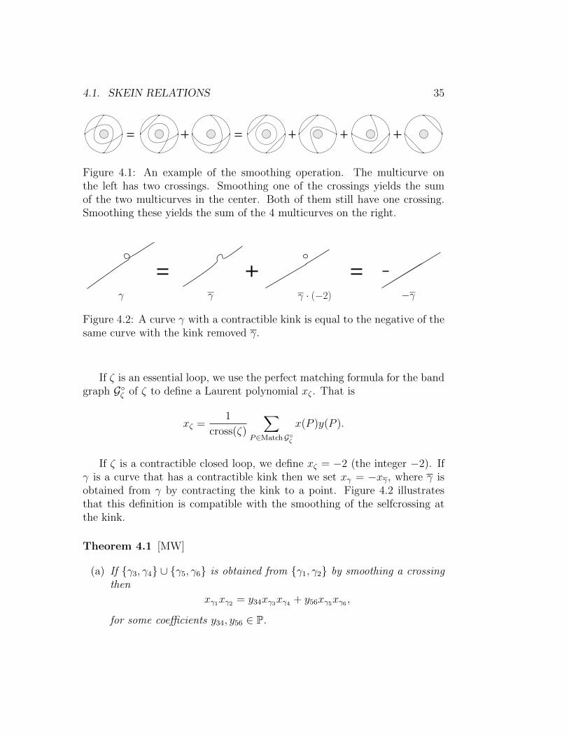
Figure 4.1: An example of the smoothing operation. The multicurve onthe left has two crossings. Smoothing one of the crossings yields the sumof the two multicurves in the center. Both of them still have one crossing.Smoothing these yields the sum of the 4 multicurves on the right.

γ γ γ · (−2) −γ

Figure 4.2: A curve γ with a contractible kink is equal to the negative of thesame curve with the kink removed γ.

If ζ is an essential loop, we use the perfect matching formula for the bandgraph G◦ζ of ζ to define a Laurent polynomial xζ . That is

xζ =1

cross(ζ)

∑P∈MatchG◦ζ

x(P )y(P ).

If ζ is a contractible closed loop, we define xζ = −2 (the integer −2). Ifγ is a curve that has a contractible kink then we set xγ = −xγ, where γ isobtained from γ by contracting the kink to a point. Figure 4.2 illustratesthat this definition is compatible with the smoothing of the selfcrossing atthe kink.

Theorem 4.1 [MW]

(a) If {γ3, γ4} ∪ {γ5, γ6} is obtained from {γ1, γ2} by smoothing a crossingthen

xγ1xγ2 = y34xγ3xγ4 + y56xγ5xγ6 ,

for some coefficients y34, y56 ∈ P.


(b) If γ34, γ56 is obtained from γ by smoothing a selfcrossing then

xγ = y34xγ34 + y56xγ56,

for some coefficients y34, y56 ∈ P.

Remark 4.2 (a) The equations in Theorem 4.1 are called skein relations.

(b) Theorem 4.1 was proved in [MW] using hyperbolic geometry. A com-binatorial proof in terms of snake and band graphs was given in [CS,CS2, CS3].

4.1.1 Smoothing of arcs vs resolutions of snake graphs

The definition of smoothing is very simple. It is defined as a local transfor-mation replacing a crossing × with the pair of segments _ (resp. ⊃⊂).But once this local transformation is done, one needs to find representativesinside the isotopy classes of the resulting curves which realize the minimalnumber of crossings with the fixed triangulation. This means that one needsto deform the obtained curves isotopically, and to ‘unwind’ them if possible,in order to see their actual crossing pattern, which is crucial for the applica-tions to cluster algebras. This can be quite complicated especially in a highergenus surface.

The situation for the snake and band graphs is exactly opposite. Thedefinition of the resolution is very complicated because one has to considermany different cases. But once all these cases are worked out, one has acomplete list of rules in hand, which one can apply very efficiently in actualcomputations. The reason for this is that the definitions of the resolutionsalready take into account the isotopy mentioned above.

For explicit computations in the cluster algebra, one always needs toconstruct the snake graphs in order to compute the Laurent polynomials.Thus for this purpose it is more efficient to work with resolutions of snakegraphs.

4.2 Definition of the bases B◦ and B.

We have seen that in order to define a basis, we need to understand productsof cluster variables, and that a product of cluster variables corresponds to a

4.2. DEFINITION OF THE BASES B◦ AND B. 37

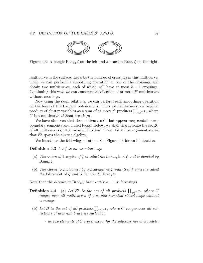
Figure 4.3: A bangle Bang4 ζ on the left and a bracelet Brac4 ζ on the right.

multicurve in the surface. Let k be the number of crossings in this multicurve.Then we can perform a smoothing operation at one of the crossings andobtain two multicurves, each of which will have at most k − 1 crossings.Continuing this way, we can construct a collection of at most 2k multicurveswithout crossings.

Now using the skein relations, we can perform each smoothing operationon the level of the Laurent polynomials. Thus we can express our originalproduct of cluster variables as a sum of at most 2k products

∏γ∈C xγ where

C is a multicurve without crossings.We have also seen that the multicurves C that appear may contain arcs,

boundary segments and closed loops. Below, we shall characterize the set B◦of all multicurves C that arise in this way. Then the above argument showsthat B◦ spans the cluster algebra.

We introduce the following notation. See Figure 4.3 for an illustration.

Definition 4.3 Let ζ be an essential loop.

(a) The union of k copies of ζ is called the k-bangle of ζ and is denoted byBangk ζ.

(b) The closed loop obtained by concatenating ζ with itself k times is calledthe k-bracelet of ζ and is denoted by Brack ζ.

Note that the k-bracelet Brack ζ has exactly k − 1 selfcrossings.

Definition 4.4 (a) Let B◦ be the set of all products∏

γ∈C xγ where Cranges over all multicurves of arcs and essential closed loops withoutcrossings.

(b) Let B be the set of all products∏

γ∈C xγ where C ranges over all col-lections of arcs and bracelets such that

- no two elements of C cross, except for the selfcrossings of bracelets;


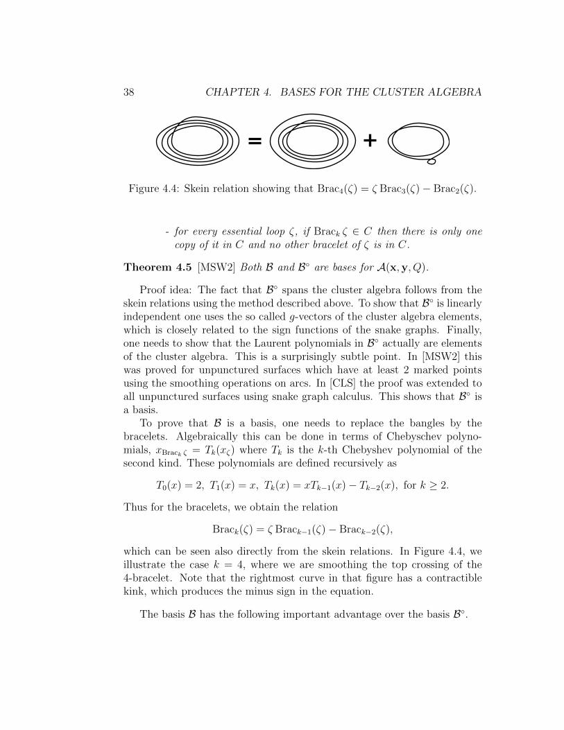
Figure 4.4: Skein relation showing that Brac4(ζ) = ζ Brac3(ζ)− Brac2(ζ).

- for every essential loop ζ, if Brack ζ ∈ C then there is only onecopy of it in C and no other bracelet of ζ is in C.

Theorem 4.5 [MSW2] Both B and B◦ are bases for A(x,y, Q).

Proof idea: The fact that B◦ spans the cluster algebra follows from theskein relations using the method described above. To show that B◦ is linearlyindependent one uses the so called g-vectors of the cluster algebra elements,which is closely related to the sign functions of the snake graphs. Finally,one needs to show that the Laurent polynomials in B◦ actually are elementsof the cluster algebra. This is a surprisingly subtle point. In [MSW2] thiswas proved for unpunctured surfaces which have at least 2 marked pointsusing the smoothing operations on arcs. In [CLS] the proof was extended toall unpunctured surfaces using snake graph calculus. This shows that B◦ isa basis.

To prove that B is a basis, one needs to replace the bangles by thebracelets. Algebraically this can be done in terms of Chebyschev polyno-mials, xBrack ζ = Tk(xζ) where Tk is the k-th Chebyshev polynomial of thesecond kind. These polynomials are defined recursively as

T0(x) = 2, T1(x) = x, Tk(x) = xTk−1(x)− Tk−2(x), for k ≥ 2.

Thus for the bracelets, we obtain the relation

Brack(ζ) = ζ Brack−1(ζ)− Brack−2(ζ),

which can be seen also directly from the skein relations. In Figure 4.4, weillustrate the case k = 4, where we are smoothing the top crossing of the4-bracelet. Note that the rightmost curve in that figure has a contractiblekink, which produces the minus sign in the equation.

The basis B has the following important advantage over the basis B◦.

4.2. DEFINITION OF THE BASES B◦ AND B. 39

Theorem 4.6 [T] The basis B has positive structure constants.

This means that if b, b′ ∈ B are two basis elements, and if we express theirproduct as a linear combination of elements in B as

bb′ =∑b′′∈B

gb′′

b,b′b”,

then the gb′′

b,b′ ∈ ZP are called the structure constants of the basis B, and the

theorem says that gb′′

b,b′ ∈ Z≥0P.

Remark 4.7 The correspondence between the cluster algebra and a triangu-lated surface can be generalized to triangulated orbifolds, see [FeShTu]. Inthis setting the cluster algebra does not correspond to a quiver but to a skew-symmetrizable matrix, and, in contrast to the surface, the orbifold is allowedto have singularities. The results in chapters 3 and 4 have been genereralizedto this setting in [FeShTu2, FeTu].


Chapter 5

Appendix: Generalization tosurfaces with punctures

5.1 Tagged arcs

Note that an arc γ that lies inside a self-folded triangle in T cannot be flipped.In order to rectify this problem, the authors of [FST] were led to introducethe slightly more general notion of tagged arcs.

A tagged arc is obtained by taking an arc that does not cut out a once-punctured monogon and marking (“tagging”) each of its ends in one of twoways, plain or notched, so that the following conditions are satisfied:

• an endpoint lying on the boundary of S must be tagged plain

• both ends of a loop must be tagged in the same way.

Thus there are four ways to tag an arc between two distinct punctures andthere are two ways to tag a loop at a puncture, see Figure 5.1. The notchingis indicated by a bow tie.

One can represent an ordinary arc β by a tagged arc ι(β) as follows. Ifβ does not cut out a once-punctured monogon, then ι(β) is simply β withboth ends tagged plain. Otherwise, β is a loop based at some marked pointq and cutting out a punctured monogon with the sole puncture p inside it.Let α be the unique arc connecting p and q and compatible with β. Thenι(β) is obtained by tagging α plain at q and notched at p.

Tagged arcs α and β are called compatible if and only if the followingproperties hold:

41

42 CHAPTER 5. APPENDIX

p q

plain

doubly notched

p q

notched at q

notched at p

p

plain doubly notched

p

Figure 5.1: Four ways to tag an arc between two punctures (left); two waysto tag a loop at a puncture (right)

62

3 4

5

1

Figure 5.2: Tagged triangulation of the punctured annulus corresponding tothe ideal triangulation of the right hand side of Figure 2.2.

• the arcs α0 and β0 obtained from α and β by forgetting the taggingsare compatible;

• if α0 = β0 then at least one end of α must be tagged in the same wayas the corresponding end of β;

• α0 6= β0 but they share an endpoint a, then the ends of α and βconnecting to a must be tagged in the same way.

A maximal collection of pairwise compatible tagged arcs is called a taggedtriangulation. Figure 5.2 shows the tagged triangulation corresponding to thetriangulation on the right hand side of Figure 2.2.

Given a surface (S,M) with a puncture p and a tagged arc γ, we let γ(p)

denote the arc obtained from γ by changing its notching at p. If p and q are

5.2. SELF-FOLDED TRIANGLES 43

pq r

`

pq r

r(p)

Figure 5.3: A self-folded triangle with loop ` and radius r (left); the cor-responding tagged arcs r and r(p) (right). In the cluster algebra we havex` = xrxr(p) .

two punctures, we let γ(pq) denote the arc obtained from γ by changing itsnotching at both p and q.

If ` is an unnotched loop with endpoints at q cutting out a once-puncturedmonogon containing puncture p and radius r, see Figure 5.3 then we set

x` = xrxr(p) .

Thus the loop is equal to the product of the two radii.

5.2 Expansion formula for plain arcs in the

presence of self-folded triangles

If there are self-folded triangles in the triangulation T then we have to modifythe y-monomials in the expansion formula of Theorem 3.4 as follows. Recallthat we had defined y(P ) as a monomial in the coefficients y1, . . . , yn andeach yi corresponds to an (untagged) arc yτi of T . Now we need to redefiney(P ) by replacing every yi in our previous definition by Φ(yi), where Φ isdefined below.

Φ(yi) =

yi if τi is not a side of a self-folded triangle;

yryr(p)

if τi is a radius r to puncture p in a self-folded triangle;

yr(p) if τi is a loop ` in a self-folded triangle with radius rand puncture p.

Then the cluster variable xγ is equal to

xγ =1

cross(γ)

∑P∈MatchGγ

x(P )y(P ).


5.3 Expansion formula for singly-notched arcs

Definition 5.1 If p is a puncture, and γ(p) is a tagged arc with a notch at pbut tagged plain at its other end, we define the associated crossing monomialas

cross(γ(p)) =cross(`p)

cross(γ)= cross(γ)

∏τ

xτ ,

where the product is over all ends of arcs τ of T that are incident to p. Ifp and q are punctures and γ(pq) is a tagged arc with a notch at p and q, wedefine the associated crossing monomial as

cross(γ(pq)) =cross(`p) cross(`q)

cross(γ)3= cross(γ)

∏τ

xτ ,

where the product is over all ends of arcs τ that are incident to p or q.

Let p be a puncture and let γ be an arc from a point q 6= p to p. Let γ(p)

be the tagged arc that is notched at p and plain at q and let ` denote theloop at q that cuts out the once-punctured monogon with puncture p andradius γ. Thus ι(`) = γ(p). Let G` be the snake graph of `.

Definition 5.2 The snake graph G` contains two disjoint connected sub-graphs, one on each end, both of which are isomorphic to Gγ. We let Gγp,1denote the one at the south west end of G` and Gγp,2 the one at the north eastend.

We let Hγp,1 be the subgraph of Gγp,1 obtained by deleting the north eastvertex, and Hγp,2 be the subgraph of Gγp,2 obtained by deleting the south westvertex.

In Figure 5.4, the subgraph Gγp,1 is the subgraph of G` consisting of thefirst two tiles and Gγp,2 is the subgraph consisting of the last two tiles. In thesame figure, the graph Hγp,1 is the graph consisting of the first tile and thesouth edge of the second tile.

Definition 5.3 A perfect matching P of G` is called γ-symmetric if the re-strictions of P to the two ends satisfy P |Hγp,1 ∼= P |Hγp,2.

If P is γ-symmetric, define

x(P ) =x(P )

x(P |Gγ,i), y(P ) =

y(P )

y(P |Gγ,i),

5.4. EXPANSION FORMULA FOR DOUBLY-NOTCHED ARCS 45

where i = 1 or 2 depending on which subgraph the restriction of P defines aperfect matching.

Let T = {τ1, . . . , τn} be a tagged triangulation of (S,M) and let A =A(xT ,yT , QT ) be the cluster algebra with principal coefficients at T . ThusxT = (x1, . . . , xn), yT = (y1, . . . , yn) and P = Trop(y1, . . . , yn).

Let p be a puncture and assume that T contains no arc notched at p. Infact this is not really a restriction, because if the arcs in T are notched at pwe can change the tags of all arcs at p to ‘plain’ and obtain the same quiverQT .

Let γ be an arc from a point q 6= p to p and let γ(p) and ` be as above.

Theorem 5.4 If γ is not in the triangulation T , then the cluster variablexγ(p) is equal to

xγ(p) =1

cross(γ(p))

∑P

x(P ) y(P ),

where the sum is over all γ-symmetric matchings P of G`.

Remark 5.5 If γ is in T (so xγ is an initial cluster variable), then sincexγ(p) = x`/xγ, where x` is computed by the formula in Theorem 3.4.

5.4 Expansion formula for doubly-notched arcs

For the case of a tagged arc with notches at both ends, we need two moredefinitions.

Let p and q be a punctures and let γ be an arc from a point p to q. Letγ(p) be the tagged arc that is notched at p and plain at q and let γ(q) be thetagged arc that is notched at q and plain at p. Let `p be the loop at q suchthat ι(`p) = γ(p), and let `q be the loop at p such that ι(`q) = γ(q).

Definition 5.6 Assume that the tagged triangulation T does not containeither γ, γ(p), or γ(q). Let Pp and Pq be γ-symmetric matchings of G`p andG`q , respectively. Then the pair (Pp, Pq) is called γ-compatible if at least oneof the following two conditinos holds.

• The restrictions Pp|Gγp,1, and Pq|Gγq,1 . are isomorphic perfect matchingsof the subgraph Gγp,1 ∼= Gγq ,1, or


• the restrictions Pp|Gγp,2, and Pq|Gγq,2 . are isomorphic perfect matchingsof the subgraph Gγp,2 ∼= Gγq ,2

If (Pp, Pq) is a γ-compatible pair of matchings define the weight and heightmonomial,

x(Pp, Pq) =x(Pp)x(Pq)

x(Pp|Gγp,i)3, y(Pp, Pq) =

y(Pp) y(Pq)

y(Pp|Gγp,i)3,

where i = 1 or 2 depending on the two cases above.

For technical reasons, we require the (S,M) is not a closed surface withexactly 2 marked points for Theorem 5.7.

Theorem 5.7 If γ is not in the triangulation T , then the cluster variablexγ(p) is equal to

xγ(pq) =1

cross(γ(pq))

∑(Pp,Pq)

x(Pp, Pq) y(Pp, Pq),

where the sum is over all γ-compatible pairs of matchings (Pp, Pq) of (G`p ,G`q).

5.5 Example of a cluster expansion for a singly-

notched arc

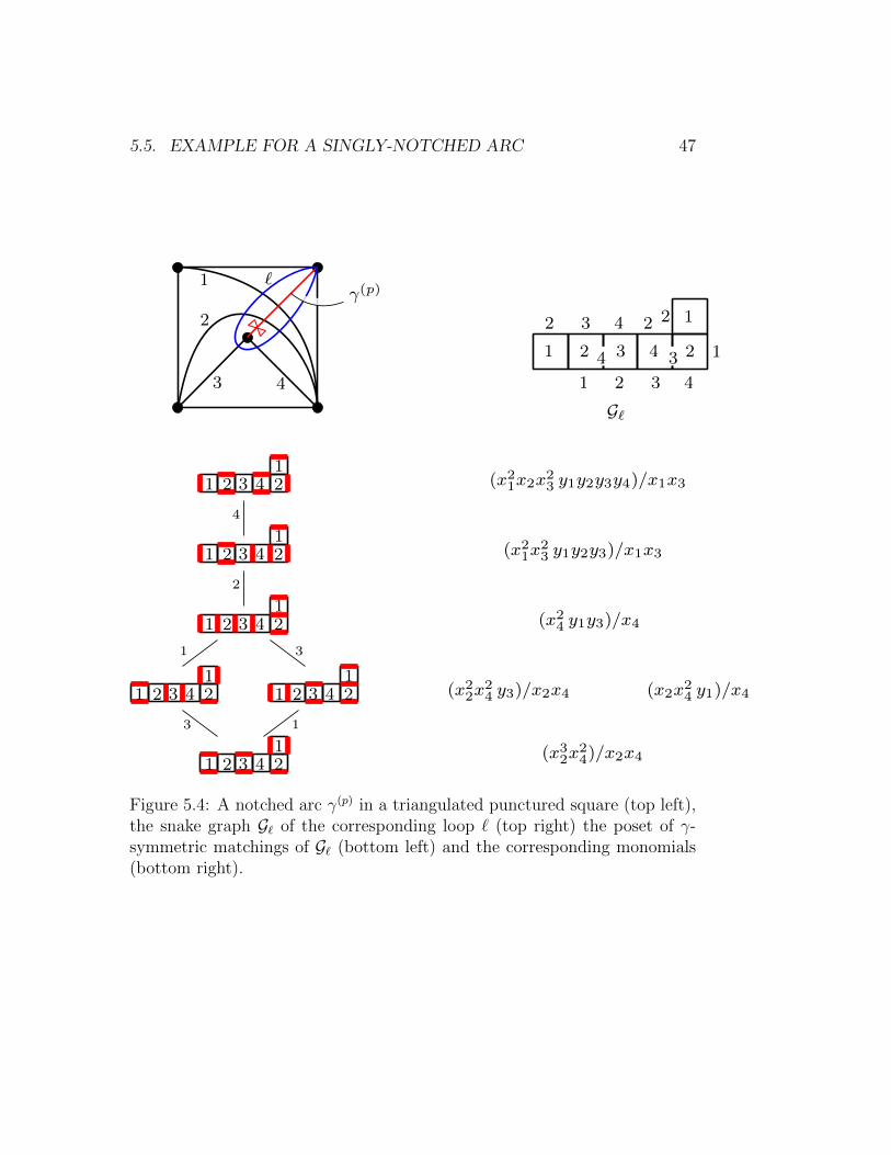
To compute the Laurent expansion of xγ(p) of the notched arc in top leftpicture in Figure 5.4, we draw the snake graph G` of the loop `, shown in thetop right picture of the same figure. The poset of γ-symmetric matchings ofG` is shown in the bottom left picture. Note that the matchings agree onthe subgraphs Hγp,1 and Hγp,2. The corresponding monomials x(P )y(P ) areshown in the bottom right of the figure.

Simplifying and dividing by cross(γ(p)) = x1x2x3x4 we obtain

xγ(p) =x1x2x3 y1y2y3y4 + x1x3 y1y2y3 + x4 y1y3 + x2x4 y3 + x2x4 y1 + x2

2x4

x1x2x3x4

.

Since all the initial variables and coefficients appearing in this sum correspondto ordinary arcs, no specialization of x-weights or y-weights was necessary inthis case.

5.5. EXAMPLE FOR A SINGLY-NOTCHED ARC 47

1 2 3 4 2

12 3 4 2 2

1 2 3 4

14 3

1 2 3 4 21

1 2 3 4 21

1 2 3 4 21

1 2 3 4 21

1 2 3 4 21

1 2 3 4 21

4

2

1 3

13

(x21x2x23 y1y2y3y4)/x1x3

(x21x23 y1y2y3)/x1x3

(x24 y1y3)/x4

(x22x24 y3)/x2x4 (x2x24 y1)/x4

(x32x24)/x2x4

γ(p)

G`

`

43

2

1

Figure 5.4: A notched arc γ(p) in a triangulated punctured square (top left),the snake graph G` of the corresponding loop ` (top right) the poset of γ-symmetric matchings of G` (bottom left) and the corresponding monomials(bottom right).


5.6 Example of a Laurent expansion for a doubly-

notched arc

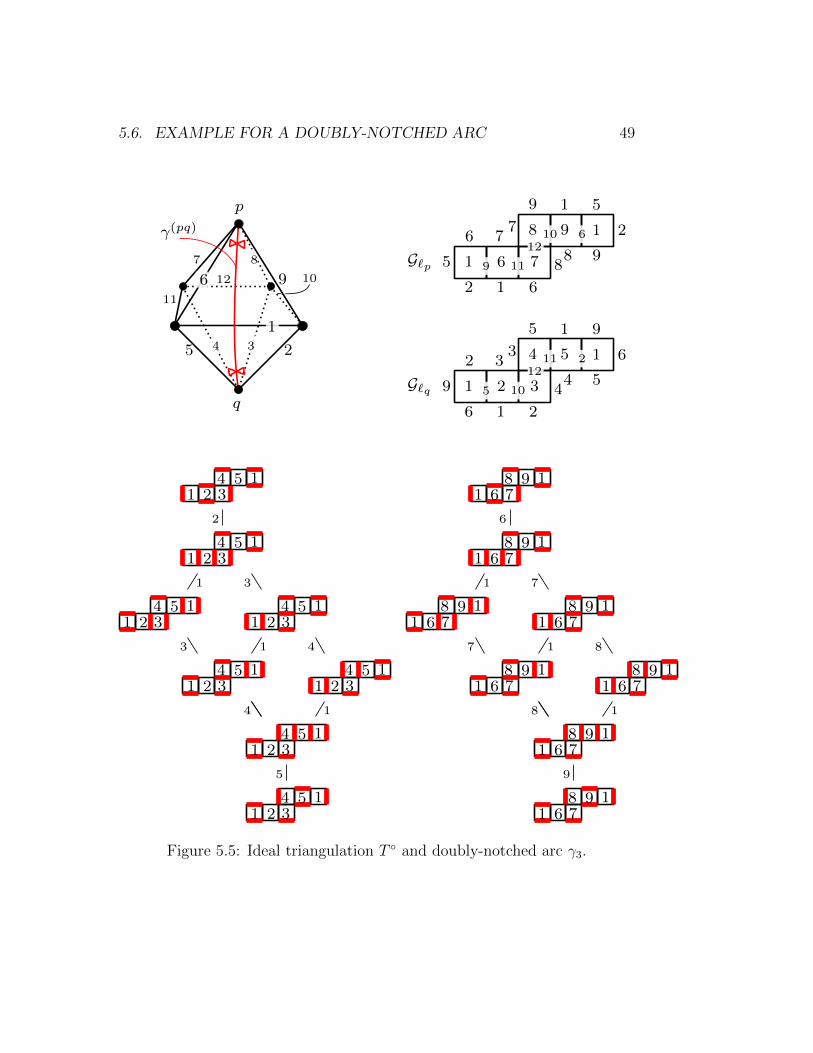
We close with an example of a cluster expansion formula for a tagged arcwith notches at both endpoints. The top left picture in Figure 5.5. shows atriangulation of a sphere with 6 punctures in the shape of an octahedron. Thenumbers 1,. . . ,12 in that figure are the labels of the arcs of the triangulation.We compute the Laruent expansion of the red arc γ(pq) in the figure. Thetwo snake graphs of the two loops `p and `q are shown in the top right ofthe figure. Note that the two snake graphs have the same shape, but not thesame labels. The pictures at the bottom of the figure show the posets of γ-symmetric matchings for both snake graphs. The corresponding monomialsx(P )y(P ) are listed below in the shape of the two posets.

x1x3x4x5x9 y1y2y3y4y5 x1x5x7x8x9 y1y6y7y8y9

x4x25x9x10 y1y3y4y5 x5x8x

29x11 y1y7y8y9

x2x4x5x6x10 y3y4y5 x2x25x9x12 y1y4y5 x2x6x8x9x11 y7y8y9 x5x6x

29x12 y1y8y9

x22x5x6x12 y4y5 x2x3x5x9x11 y1y5 x2x26x9x12 y8y9 x5x6x7x9x10 y1y9

x22x3x6x11 y5 x2x26x7x10 y9

x1x2x3x4x6 x1x2x6x7x8

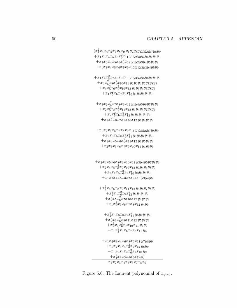
We want to find all γ-compatible pairs. The four perfect matchings onthe lower left side of the first poset all have horizontal edges on the first tile.These edges have labels 2 and 6. Therefore, each of these matchings formsa γ-compatible pair with each of the four matchings on the lower left side ofthe second poset. Similarly, the four perfect matchings on the upper rightside of the first poset all have horizontal edges on the last tile. These edgeshave labels 5 and 9. Therefore, each of these matchings forms a γ-compatiblepair with each of the four matchings on the upper right side of the secondposet. There are no other γ-compatible pairs, so we have a total of 32 pairs.The Laurent polynomial for xγ(pq) is shown in Figure 5.6.

5.6. EXAMPLE FOR A DOUBLY-NOTCHED ARC 49

1

5

1 2 34 5 1

2

γ(pq)

p

q

3 2

96

7

4

8

11

1012

1 2 3

4 12 3

1 2

10G`q

5

5

1211 2

3

4 54

15

9

6

9

6

1 6 7

8 16 7

1 6

11G`p

9

9

1210 6

7

8 98

19

5

2

5

2

1 2 34 5 1

1 2 34 5 1

1 2 34 5 1

1 3

1 2 34 5 1

3 1

1 2 34 5 1

4

1 2 34 5 1

5

1 2 34 5 1

4

1

1 6 78 9 1

6

1 6 78 9 1

1 6 78 9 1

1 6 78 9 1

1 7

1 6 78 9 1

7 1

1 6 78 9 1

8

1 6 78 9 1

9

1 6 78 9 1

8

1

Figure 5.5: Ideal triangulation T ◦ and doubly-notched arc γ3.


(x21x3x4x5x7x8x9 y1y2y3y4y5y6y7y8y9

+x1x3x4x5x8x29x11 y1y2y3y4y5y7y8y9

+x1x3x4x5x6x29x12 y1y2y3y4y5y8y9

+x1x3x4x5x6x7x9x10 y1y2y3y4y5y9

+x1x4x25x7x8x9x10 y1y3y4y5y6y7y8y9

+x4x25x8x

29x10x11 y1y3y4y5y7y8y9

+x4x25x6x

29x10x12 y1y3y4y5y8y9

+x4x25x6x7x9x

210 y1y3y4y5y9

+x1x2x25x7x8x9x12 y1y4y5y6y7y8y9

+x2x25x8x

29x11x12 y1y4y5y7y8y9

+x2x25x6x

29x

212 y1y4y5y8y9

+x2x25x6x7x9x10x12 y1y4y5y9


+x2x3x5x8x29x

211 y1y5y7y8y9

+x2x3x5x6x29x11x12 y1y5y8y9

+x2x3x5x6x7x9x10x11 y1y5y9


+x2x4x5x26x9x10x12 y3y4y5y8y9

+x2x4x5x26x7x

210 y3y4y5y9


+x22x5x6x8x9x11x12 y4y5y7y8y9

+x22x5x

26x9x

212 y4y5y8y9

+x22x5x

26x7x10x12 y4y5y9

+x1x22x5x6x7x8x12 y4y5

+x22x3x6x8x9x

211 y5y7y8y9

+x22x3x

26x9x11x12 y5y8y9

+x22x3x

26x7x10x11 y5y9

+x1x22x3x6x7x8x11 y5


+x1x2x3x4x26x9x12 y8y9

+x1x2x3x4x26x7x10 y9

+x21x2x3x4x6x7x8)

x1x2x3x4x5x6x7x8x9

Figure 5.6: The Laurent polynomial of xγ(pq) .

Bibliography

[CCS1] P. Caldero and F. Chapoton and R. Schiffler, Quivers with relationsarising from clusters (An case), Trans. Amer. Math. Soc. 358 (2006), no.3, 1347-1364.

[CLS] I. Canakci, K. Lee and R. Schiffler, On cluster algebras from unpunc-tured surfaces with one marked point, Proc. Amer. Math. Soc. Ser. B 2(2015) 35–49.

[CS] I. Canakci and R. Schiffler, Snake graph calculus and cluster algebrasfrom surfaces, J. Algebra, 382, (2013) 240–281.

[CS2] I. Canakci and R. Schiffler, Snake graph calculus and cluster algebrasfrom surfaces II: Self-crossing snake graphs, Math. Z. 281 (1), (2015),55-102.

[CS3] I. Canakci and R. Schiffler, Snake graph calculus and cluster algebrasfrom surfaces III: Band graph and snake rings, arXiv:1506.01742.

[FeShTu] A. Felikson, M. Shapiro, P. Tumarkin. Skew-symmetric cluster al-gebras of finite mutation type, J. Eur. Math. Soc. 14, (2012), no. 4, 1135–1180.

[FeShTu2] A. Felikson, M. Shapiro, P. Tumarkin. Cluster algebras and tri-angulated orbifolds. Adv. Math. 231 (2012), no. 5, 2953–3002.

[FeTu] A. Felikson, M. Shapiro, P. Tumarkin. Bases for cluster algebras fromorbifolds. arXiv:1511.08023.

[FG1] V. Fock and A. Goncharov, Moduli spaces of local systems and higherTeichmuller theory. Publ. Math. Inst. Hautes Etudes Sci. 103, (2006), 1–211.

51

52 BIBLIOGRAPHY

[FG2] V. Fock and A. Goncharov, Cluster ensembles, quantization and thedilogarithm, Ann. Sci. Ec. Norm. Super. (4) 42 (2009), no. 6, 865–930.

[FG3] V. Fock and A. Goncharov, Dual Teichmuller and lamination spaces.Handbook of Teichmuller theory. Vol. I, 647–684, IRMA Lect. Math.Theor. Phys., 11, Eur. Math. Soc., Zurich, 2007.

[FST] S. Fomin, M. Shapiro, and D. Thurston, Cluster algebras and triangu-lated surfaces. Part I: Cluster complexes, Acta Math. 201 (2008), 83–146.

[FT] S. Fomin and D. Thurston, Cluster algebras and triangulated surfaces.Part II: Lambda Lengths, preprint (2008),

[FZ1] S. Fomin and A. Zelevinsky, Cluster algebras I: Foundations, J. Amer.Math. Soc. 15 (2002), 497–529.

[FZ2] S. Fomin and A. Zelevinsky, Cluster algebras II: Finite type classifica-tion, Invent. Math. 154 (2003), 63–121.

[FZ4] S. Fomin and A. Zelevinsky, Cluster algebras IV: Coefficients, Com-positio Mathematica 143 (2007), 112–164.

[GSV] M. Gekhtman, M. Shapiro and A. Vainshtein, Cluster algebras andWeil-Petersson forms, Duke Math. J. 127 (2005), 291–311.

[LF] D. Labardini-Fragoso, Quivers with potentials associated to triangu-lated surfaces, Proc. Lond. Math. Soc. (3) 98, (2009), no. 3, 797–839

[LS] K. Lee and R. Schiffler, Positivity for cluster algebras, Ann. Math. 182(1), (2015) 73–125.

[MS] G. Musiker. R. Schiffler, Cluster expansion formulas and perfect match-ings, J. Algebraic Combin. 32, (2010), no. 2, 187–209.

[MSW] G. Musiker, R. Schiffler and L. Williams, Positivity for cluster alge-bras from surfaces, Adv. Math. 227, (2011), 2241–2308.

[MSW2] G. Musiker, R. Schiffler and L. Williams, Bases for cluster algebrasfrom surfaces, Compos. Math. 149, 2, (2013), 217–263.

[MW] G. Musiker and L. Williams, Matrix formulae and skein relations forcluster algebras from surfaces, Int. Math. Res. Not. 13, (2013), 2891–2944.

BIBLIOGRAPHY 53

[Pr] J. Propp, The combinatorics of frieze patterns and Markoff numbers,preprint, arXiv:math.CO/0511633.

[S] R. Schiffler, A cluster expansion formula (An case), Electron. J. Combin.15 (2008), #R64 1.

[S2] R. Schiffler, On cluster algebras arising from unpunctured surfaces II,Adv. Math. 223, (2010), no. 6, 1885–1923.

[ST] R. Schiffler and H. Thomas. On cluster algebras arising from unpunc-tured surfaces, Int. Math. Res. Notices. (2009) no. 17, 3160–3189.

[T] D. Thurston, Positive basis for surface skein algebras. Proc. Natl. Acad.Sci. USA 111 (2014), no. 27, 9725–9732.

Documents

Cluster algebras from surfaces - UCONNschiffler/LNCIMPA.pdf · 2.3 Cluster algebras from surfaces ... polynomials in the variables y 1 ... Let Xbe the set of all cluster variables