Climate change impacts on and adaptation measures for agriculture in Austria in 2020: Linking bottom‐up and top‐

down models 

Birgit Bednar-Friedl1,2, Olivia Koland1*, Erwin Schmid3, Martin Schönhart3

1 University of Graz, Wegener Center for Climate and Global Change 2 University of Graz, Department of Economics 3 University of Natural Resources and Life Sciences, Institute for Sustainable Economic Development, Vienna * Corresponding author: E-mail: olivia.koland@uni-graz.at

ABSTRACT: Agriculture is among the economic sectors most exposed to global climate change and the impacts are likely transmitted to other economic sectors. The main objective of this paper is to present the interface between a sectoral bottom-up and a computational general equilibrium (CGE) top-down modeling approach. This approach allows better assessing the impacts of climate change on agriculture and its inter-sectoral responses in the Austrian economy. Model results from the sectoral bottom-up model and four regional climate models show mixed results, i.e. agricultural production gains and losses depending on the climate change scenarios and NUTS-3 regions. Agricultural adaptation measures increase gains or reduce losses, and are transmitted to other sectors in the economy.

Keywords: bottom-up to top-down, agriculture, climate change impacts, adaptation

1. Introduction

Exposure to climate change is one of the major challenges to agriculture in the next decades. Changing climatic and weather conditions affect crop yields and may lead to higher and more volatile prices (FAO/OECD 2010). Yet, sectoral vulnerability is not only determined by exposure to changing climatic conditions and by its sensitivity to this changes but also by the capability to adapt to a changing environment (Bindi and Olesen, 2010; IPCC, 2001). Adaptation depends on technical and economic factors (availability of technologies, growing demand, sectoral dependencies etc.), farmers attitudes and management capacities, as well as political framework conditions (e.g. agricultural and environmental policies) (Fleming and Vanclay, 2010; Reidsma et al., 2010; Reidsma et al., 2009). To account for the cross-cutting nature of sectoral adaptation, an integrated modeling approach - combining agricultural adaptation and macroeconomic feedback effects - is required.

Traditionally, agriculture is a highly subsidized and regulated sector in order to meet multiple sectoral and societal objectives (e.g. international competitiveness, food security, farm incomes, and environmental quality). The assessment of adaptation measures in response to climate, whether taken autonomously by farmers or policy-

2

induced, needs to take account of these policy objectives as well as of sectoral spill-over effects. The main objective of this paper is thus to assess the impacts of and response options to climate change for the Austrian agricultural sector and the transmitted effects to the national economy. Austria is an interesting case due to its heterogeneous agricultural production conditions, with areas located in both lowlands and alpine regions.

To assess the climate change impacts and adaptation for Austrian agriculture in 2020, we link a bottom-up sectoral model to a top-down economy-wide model. In the literature, different kind of agricultural sector models have already been linked with GTAP based models. For instance, GTAP has been linked with partial equilibrium models for the agricultural sector (such as CAPRI, see e.g. Jansson et al., 2009; Britz and Hertel, 2009), or crop models providing physical crop yields (such as IMAGE, see e.g. van Meijl et al., 2006). There are also several examples for linking land use optimization models such as PASMA and partial equilibrium models (see for example the link between FSSIM and SEAMCAP in the SEAMLESS project, van Ittersum et al., 2008).

In our application, we link the agricultural production model PASMA (Schmid and Sinabell 2007) with a national-scale multi-sector computable general equilibrium (CGE) model for Austria based on the GTAP 7 database. PASMA maximizes total gross margins from land use and livestock activities in all Austrian NUTS-3 regions. PASMA depicts the natural, structural and economic heterogeneity in Austrian farming in detail The CGE model is less detailed in agriculture, but represents the whole economy including its interdependencies between economic sectors, private consumption, international trade relations and policies.

The main challenge of linking the two models is consistency. Since PASMA is a pure supply model in contrast to the general equilibrium structure of the CGE model, PASMA results will never coincide perfectly with their corresponding CGE outputs such as the value of total agricultural production. This is true even if data, scenario assumptions and structural parameters are made consistent as far as possible. A main focus of model linking will thus be laid on the base year and future BAU calibrations.

Besides the considerable challenges, linking of the two models may lead to significant knowledge gains. PASMA takes economic and political developments such as anticipated results of the ongoing CAP reform into account. Comparing against these developments, climate change effects of increasing temperatures and changing precipitation levels are expected to remain modest in the near future (e.g. 2020). With a time horizon of 2050, higher temperatures and changes in precipitation may more significantly affect crop yields (cf. IPCC, 2007) and related livestock production, which are both considered in PASMA and passed on to the CGE model.

This article is structured as follows. Section 2 briefly describes the structure of the two models and the modeling interfaces. Climate change and adaptation scenarios are outlined in section 3, while section 4 presents key results for agriculture and the Austrian economy. Section 5 summarizes and concludes.

3

2. Methods and model specifications

The core of the modeling approach consists of a bottom-up to top-down model interface that couples an agricultural land use optimization model (PASMA, Schmid and Sinabell, 2007) with a CGE model for the Austrian economy based on the GTAP 7 database (GTAP, 2007).

2.1 The sectoral supply model for agriculture in Austria

PASMA is an economic land use optimization model for agriculture in Austria (Schmid and Sinabell, 2007; Schmidt et al., 2012). It maximizes total gross margins from observed and alternative land use and livestock activities for all Austrian NUTS-3 regions. Positive mathematical programming is applied to calibrate the model to observed production with respect to livestock and land use levels as well as intensities. PASMA portrays the natural, structural, economic, and policy contexts of Austrian agriculture in detail. Particularly, the first and second pillars of CAP are considered including the Single Farm Payments and other direct payments, measures of the Austrian agri-environmental program ÖPUL, and less favoured area payments. Consequently, PASMA has its strength in its detailed description of the farming systems with respect to regionally disaggregated farm structures, bio-physical properties, and agricultural policies. It has been made consistent with the Austrian agricultural statistics. PASMA is validated against the economic accounts of agriculture (Statistics Austria, 2011b).

Climate change effects are considered in PASMA via spatially explicit crop yield simulations using the biophysical process model EPIC (Williams, 1995). EPIC has been applied on homogeneous response units (HRU) – a spatial representation of the topographical and soil characteristics in Austria - using regional climate change scenarios and crop management variants. Each HRU is assumed to be homogeneous with respect to soil type, slope, and altitude at a spatial resolution of one to several km². In total, we have delineated 443 HRUs for Austria. Climate change data is provided from four contrasting regional climate models (RCM) along a precipitation as well as temperature gradient. The crop management variants consist of alternative crop rotations and fertilization and irrigation regimes as well as reduced tillage and winter cover cropping systems.

Thus, PASMA provides detailed sectoral data on all major land use and livestock activities in order to replace less detailed GTAP-input data as well as to account for climate change impacts on agriculture.

2.2 The CGE model for the Austrian economy

The CGE model has less detail both in terms of agricultural crops (for plant and three livestock sectors) and spatial resolution (NUTS-1) than the sector model, but captures the impact of changes in agriculture on the rest of the economy and arising feedback effects on the agricultural sector.

4

The CGE model builds on the GTAP 7 database. GTAP 7 is a unique global database developed by the Centers for Global Trade Analysis (Purdue University) representing input tables for 113 countries and 57 sectors which are consistent in their international trade flows. An additional advantage compared to the national input output table released by Statistics Austria is its high sectoral detail in agriculture (12 agricultural sectors, thereof eight crop and four livestock sectors). Since for Austria some agricultural sectors are of no or minor importance (such as rice), the eight crop sectors were aggregated to four. The GTAP livestock sectors were disaggregated in such a way that the importance of cattle and milk production in Austria is being considered. Table 1 gives more details on the sectoral structure of the CGE model, where in addition to agriculture those sectors are considered which are either important as inputs for agriculture or are of high relevance for Austria’s economy such as electricity, energy intensive production, transport, and services.

Table 1: Sectoral aggregation of CGE model

Sectors Code Sectors Code

Agricultural (land using) sectors

Crop sectors (land using) Livestock sectors

Wheat and meslin, cereal grains nec. GRA Cattle CTL

Vegetable and fruits VAF Milk RMK

Oil seeds OSD Other animal products OAP

Crops nec. OCR

Resource using sectors

Energy carriers NRG Mining OMN

Forestry FRS Fishing FSH

Non-resource using sectors

Electricity ELY Rest of energy intensive industry REIS

Chemicals CRP Rest of industry NEIS

Petroleum products PC Food products FOOD

Other transport OTP Trade TRD

Water transport WTP Insurance ISR

Air transport ATP Recreational services ROS

Real estate and renting OBS Rest of services/utilities SEV

Following the structure of agents used in the social accounting matrix (SAM) generated by GTAP, the so-called regional household is an aggregate of private and public households and thus represents total final demand. This regional household provides the primary factors capital, labor, land and natural resources for the 25 sectors, and receives total income including various tax revenues. The regional household redistributes this stream of income between the private household demand, public demand and investment.

Following the Armington hypothesis (Armington, 1969), domestic output and imported goods are imperfect substitutes. Armington elasticities are based on GTAP (2007).

5

Austria is modeled as a small open economy without influence on world market prices. Labor, capital, and land are mobile within the economy but immobile across borders. The supply of production factors is essential within climate change impact and adaptation processes: land is vital within agriculture, while capital is important for large-investment adaptation projects and long-term adjustments.

There are three types of production activities which differ slightly in their production functions: (i) agricultural, land using sectors, (ii) resource using (primary energy) extraction sectors, and (iii) non-resource using commodity production. Agricultural crop sectors (GRA, VAF, OSD, OCR) are characterized by land as a factor input. In resource using sectors (NRG, FRS, OMN, FSH), a specific resource input is used. For all types of production activities, nested constant elasticity of substitution (CES) production functions with several levels are employed to specify the substitution possibilities in domestic production between primary inputs, intermediate energy and material inputs as well as the substitutability between energy commodities. At the top level of land using sectors, output is produced with a very low elasticity of substitution (s:0.1) between land and a non-land composite to acknowledge the fixed factor land. Substitution elasticities between intermediate inputs in agriculture are set greater than zero for livestock sectors where different fodder crops and animal feeds are plausible. A greater than zero elasticity of substitution between the labour/capital/energy-composite and intermediate is chosen to reflect substitution between e.g. labour/capital and pesticides. Final demand is determined by consumption of the private household and the government. Both the private household and the government maximize utility subject to their disposable income received from the regional household. Consumption of private households in each region is characterized by a constant elasticity of substitution between a material consumption bundle and an energy aggregate. Public consumption is modeled as a Cobb Douglas aggregate of an intermediate material consumption bundle.

2.3 The model interface: transmission of agricultural policy, climate change impacts, and adaptation options

PASMA and the CGE model are linked to utilize their individual advantages. The main modeling challenges include ensuring consistency of structural and technological parameters (such as intermediate input structure including imports and factor intensities) and agricultural supply and price levels. In general, four steps are necessary to link the two models: (i) defining linking items (parameters and variables to be homogenized) (ii) establishing a map between PASMA activities and CGE sectors (on input and output side), (iii) development of algorithms that send the information over the link, and (iv) providing consistency between exogenous model assumptions and parameters. As for (iii), there are two possible directions: upward interface (from sector model PASMA to CGE model) and downward interface (from CGE to PASMA) (cf. Jannsson et al, 2009).

Thus, such an interface needs to acknowledge different model structures as well as data stratifications. For example, PASMA output represents livestock as well as land use activities such as the production of one hectare of wheat with a certain management. This bio-physical output is priced and aggregated to a specific plant sector, such as that

6

for grain production (GRA) in the CGE model. At the level of production inputs, a single value for variable production costs in PASMA had to be disaggregated to different intermediary input sectors. With respect to capital demand for farm buildings and machinery, coefficients have been derived for all PASMA activities from the farm accounting data network (FADN) in Austria (LBG, 2010) and used to determine the amount of capital used in the sectors (see Figure 1).

Figure 1: Linking the agricultural supply model with the CGE model of the Austrian economy

2.3.1 Base year calibration and mapping of sectors, production factors and subsidies

The static multi-sectoral CGE model is calibrated to the year 2004. For this base year calibration, bottom-up data of PASMA is mapped and made consistent with the CGE model data base by applying SAM (Social Accounting Matrix) balancing routines. In doing so, specific constraints on SAM flows ensure that only little information from PASMA is lost in the balancing process. To achieve this, it is necessary to handle negative values, which occur e.g. in case of subsidies to the agricultural sectors, correctly (cf. Robinson and El-Said, 2000 a,b). Since GTAP is denoted in USD 2004 values while PASMA reports in EUR at nominal values for the period 2006-2008, also price level and exchange rate differences between the data bases need to be adjusted accordingly (the inflation rate is assumed at 1.96% p.a. based on the OECD consumer price index for food, http://stats.oecd.org/; the EUR/USD exchange rate is assumed at 0.8286 based on own calculations with national accounts in EUR relative to GTAP data in USD). Where detailed

7

information from the sector model is not available, the most reliable data sources (national accounts, import statistics) are used to complete (and validate) the CGE calibration process for 2004. Ultimately, the calibration process reproduces the (price adjusted) agricultural supply levels 2004 as reported by PASMA.

While industry structures for non-agricultural sectors reflect patterns of consumption and technology common across countries, for agriculture geographic factors such as climate and soil influence the industry structure heavily. A crucial point in the interface is therefore sectoral mapping. Each PASMA output activity is thus assigned to one of the seven agricultural sectors (see Table 7), while each intermediate input, expressed in variable production costs in PASMA, is matched with one agricultural or non-agricultural GTAP sector (see Table 8). According to Jensen (s.a.), hectare and set aside premiums for arable crops are allocated under land-based payments; payments for livestock production are allocated under capital-based payments. Moreover, the sector division of labour (approximated in labour units (hours) in PASMA), capital (approximated via depreciation rates of fixed production inputs in PASMA) and land (in ha) is being considered in the SAM balancing routine.

2.3.2 Calibrating to an integrated Business-as-Usual scenario 2020

In PASMA, the BAU considers major changes in the agricultural policy environment and changes in market prices for farm inputs and outputs. Agricultural policy changes include the shift in direct payment system from historical to regional entitlements, the introduction of obligatory environmental management measures as prerequisite for such payments, as well as reductions in premiums within the second pillar of the CAP, i.e. for agri-environmental payments and less developed area payments. Furthermore, we integrate the liberalized milk market as a consequence of phasing out the dairy quota system.

In the CGE model, three key drivers trigger economic development: (i) factor development (capital stock development, +1.3% p.a. according to Poncet, 2006; work force growth, +0.08% p.a. according to Statistics Austria, 2011; land area development, -0.27% p.a. on average according to exogenously assumed land use shifts towards building areas and decreasing subsidy levels in PASMA), (ii) multi factor productivity (MFP) growth (based on EU-KLEMS database 1995-2004 for non-agricultural sectors, see Appendix) and (iii) autonomous energy efficiency improvements (AEEI) (1% p.a. based on Boehringer, 1999). These average annual growth rates are implemented for 16 years yielding the BAU 2020.

The key aim for establishing an integrated Business-as-Usual scenario (BAU) 2020 is ensuring consistency in sectoral output levels for each of the seven agricultural sectors. To achieve this consistency (upward model interface passing values from PASMA to the CGE model), the following adjustments were made in the CGE model: First, land use change per sector was matched with PASMA values. Moreover, the shift in agricultural subsidization regime by 2020 was considered by changing the different subsidy rates for each agricultural sector. Land-based subsidies (applied in crop sectors) were modeled as input subsidies, while changes in capital-based subsidies (applied in livestock sectors)

8

may have a more direct output response and were thus considered as output subsidies (cf. Bach et al., 2000). Second, also the altered cost structure by 2020 was passed on to the CGE model. Third and finally, multi-factor-productivities in the agricultural sectors were adjusted in such a way that in the BAU 2020 sector outputs are consistent with values reported by PASMA (for the resulting MFPs see Table 9 in the Appendix).

2.3.3 Linking climate change impact and adaptation information

As PASMA integrates crop yields from EPIC simulations, climate change impacts on crop production in 2020 are transmitted to the CGE model to analyze general equilibrium consequences of adaptation via the established model interface. In addition to changed crop yields and hence output, PASMA allows for (minor) behavioral changes by the farmer responding to climate change. We thus call this scenario “climate change impacts with minimal adaptation”. To achieve the agricultural output levels generated by PASMA, in the CGE model different sectoral MFP rates are applied in all agricultural sectors.

In addition to climate change impacts, autonomous adaptation will be considered. The model system is also capable of investigating policy-induced adaptation, which will be carried out hereafter.

3. Climate change impact and adaptation scenarios

The models are applied in a scenario analysis considering four regional climate scenarios and two adaptation scenarios for the year 2020 leading to 8 scenario runs apart from the base run simulation and the BAU runs for 2020.

The adaptation scenarios are developed on a gradient from minimal adaptation (“dumb farmer”) to autonomous adaptation (“clairvoyant farmer”; cf. Schneider et al., 2000).

3.1 Climate change impacts with minimal adaptation (Scenario 1)

The contrasting climate scenarios are based on the results of four regional climate models, which are driven by four different global climate models. These simulations have been chosen to take into account some of the uncertainties inherent to climate modeling (cf. Heinrich and Gobiet, 2011). In comparison to the average of all 22 climate simulations of the ENSEMBLES project (www.ensembles-eu.org), two simulations yield warmer conditions and either wetter (CNRM_RM4.5) or drier conditions (ETHZ_CLM) between the periods 1961-1990 and 2021-2050, while two simulations are colder and either wetter (ICTP_RegCM) or drier (SMHI_RCA) respectively. Climate change effects are integrated in the modeling system via changes in crop yields. However, one must keep in mind that we consider changes within the two time periods for each climate simulation individually. Figure 2 presents grassland yield changes for the climate simulations at NUTS-3 level.

9

Figure 2: Average changes in grassland yields [in %] between the periods 2003-2012 and 2016-2025 at NUTS-3 level for four different regional climate scenarios

Naturally, farmers respond spontaneously to changing climate conditions depending on their awareness, risk attitudes, management skills, financial constraints and other factors. These reactions include e.g. choices on crop species, crop management (e.g. tillage, fertilizer application, and irrigation), or farm investments (e.g. irrigation infrastructure). In a first impact scenario, however, we assume a situation with only limited adaptation to the changing climate, including choices on plant sowing and harvesting dates and adjustments of livestock numbers. However, no shift in technology or crop species is allowed. This reveals the economic impacts of climate change on agriculture and its corresponding vulnerability.

3.2 Autonomous adaptation (Scenario 2)

The autonomous adaptation scenario rests on the impact scenario. In PASMA, changes among crop species and land use intensities now become possible as well. Consequently, the model can shift production to crops which are better adapted to the new climate situation. For example, more winter crops, such as winter wheat, can be produced if the winter season becomes wetter and warmer and the summer season drier and hotter. Adaptation in land use intensity includes adjustment of fertilizer application levels.

10

Improving or deteriorating growing conditions affects the crop yield potentials of a location, which may lead to input adjustments.

4. Results

Given the BAU and impact scenarios reported on sector level by PASMA, we report on the effects of structural and policy changes (BAU 2020 compared to 2004) and of climate change impacts and autonomous adaptation (2020 scenarios compared to BAU 2020) both within and outside the agricultural sector.

4.1 The Business-As-Usual situation 2020

4.1.1 Effects on Austrian agriculture

Due to productivity gains, many agricultural sectors show stagnating or increasing production quantities between the base year (2004) and BAU (2020). Nevertheless, most agricultural products face declining real prices compared to the base run period, which are not offset by increasing output quantities. Declining prices result from productivity gains, from termination of EU market price support, and a low price elasticity of demand. Consequently, agricultural outputs decrease in all agricultural sectors except OSD (shown in Figure 4). This is in line with past trends (see for example Eurostat data base: economic accounts for agriculture).

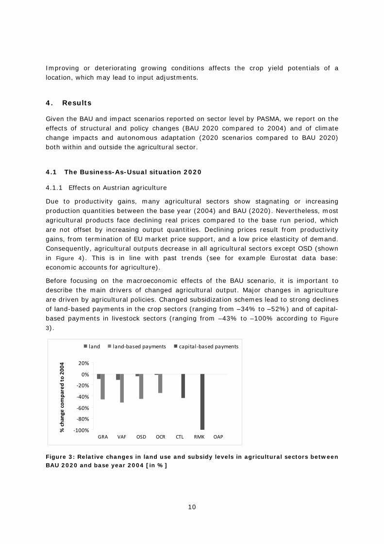
Before focusing on the macroeconomic effects of the BAU scenario, it is important to describe the main drivers of changed agricultural output. Major changes in agriculture are driven by agricultural policies. Changed subsidization schemes lead to strong declines of land-based payments in the crop sectors (ranging from –34% to –52%) and of capital-based payments in livestock sectors (ranging from –43% to –100% according to Figure 3).

‐100%

‐80%

‐60%

‐40%

‐20%

0%

20%

GRA VAF OSD OCR CTL RMK OAP

% change compared to 200

4

land land‐based payments capital‐based payments

Figure 3: Relative changes in land use and subsidy levels in agricultural sectors between BAU 2020 and base year 2004 [in %]

11

Abolishment of the milk quota regime increases milk production quantities by about 15%. However, declining real prices still reduce the output of sector RMK. In CTL, constant production quantities and declining prices lead to considerable losses in production value. Furthermore, agricultural land resources decrease by about 4.4% on average due to exogenously assumed land use shifts of agricultural land to building areas and decreasing subsidy levels, which is again important for crop sectors.

4.1.2 Effects on the Austrian economy

Output declines in six of the seven agricultural sectors and the slight increase in OSD feed back to the overall economy and its performance 2020 (Figure 4). The outcome of the non-agricultural sectors in 2020 is also influenced by developments of multi-factor-productivity growth and efficiency improvements, and for some sectors the productivity effects might be clearly the dominating ones (compared to the spillover effects from agriculture).

‐60%

‐40%

‐20%

0%

20%

40%

60%

NRG ELY

CRP PC

REIS

NEIS

OTP

WTP ATP

GRA VAF

OSD

OCR CTL

RMK

OAP

FOOD

FRS

OMN

FSH

TRD

ISR

OBS

ROS

SEV

% change compared to 200

4

BAU 2020

Sector codes: NRG = energy carriers, ELY = electricity, CRP = chemicals, PC = petroleum products, REIS = rest of energy intensive industry, NEIS = rest of industry, OTP/WTP/ATP = other/water/air transport, GRA = grain, VAF = vegetable & fruits, OSD = oil seeds, OCR = other crops, RMK = milk, CTL = cattle, OAP = other animal products, FOOD = food, FRS = forestry, OMN = mining, FSH = fishing, TRD = trade, ISR = insurance, OBS = real estate and renting, ROS = recreational services, SEV = rest of services/utilities

Figure 4: Relative changes in agricultural and economy-wide sector output between BAU 2020 and base year 2004 [in %]

The most important non-agricultural sector connected to the agricultural ones is food. Although the food industry is characterized by strong linkages to agriculture, particularly as main downstream industry, its production level rises by 2020 compared to 2004.The reason is productivity gains for food and its largest supplier (TRD). The increase of the food sector is however slowed down by the production declines in agriculture. Energy sectors (NRG, ELY, PC) are subject to an autonomous efficiency improvement of 1% per year. Resource using sectors (FRS, OMN, FSH, NRG) are supposed to have multi-factor-productivity gains. In the service sectors (ISR, OBS, ROS, SEV), a combination of high

12

labour intensity (SEV) or capital intensity (OBS), respectively, with low Armington elasticities in trade (steering imports/exports from/to the rest of the world endowed with a slight productivity increase also in services) lead to rising output levels by 2020.

4.2 Impacts from climate change (Scenario 1)

4.2.1 Impacts on agriculture

Compared to the BAU scenario 2020, the climate change scenarios considered lead to increases or decreases in production values, depending on the underlying scenario. When impacts are triggered by a rather favorable climate scenario for crop and livestock production in Austria (such as the ETHZ_CLM climate scenario), a positive effect on output levels emerges for all agricultural sectors by 2020.

Table 2: Changes of agricultural output values and producer rents in scenario 1 from BAU (in %) for four climate simulations and all agricultural sectors for the year 2020

Agricultural Producer Rent

GRA VAF OSD OCR CTL RMK OAP SUM SUMICTP_RegCM 2% 2% 2% 1% 5% 6% 3% 3% 1.4%CNRM_RM4.5 ‐2% ‐1% ‐1% 0% 0% 0% 0% ‐1% ‐0.8%ETHZ_CLM 3% 4% 3% 3% 6% 8% 3% 5% 2.4%SMHI_RCA 3% 1% 2% 1% 2% 3% 1% 2% 0.8%

Production Value

Notes: Scenario 1 reproduces the BAU land use with crop yields based on the climate simulations. The seven agricultural sectors include four plant production sectors (GRA: grain, VAF: vegetables and fruits, OSD: legumes and oilseeds, OCR: other crops including forage) and three livestock sectors (RMK: dairy products, CTL: cattle, OAP: other animal production including hogs and poultry). SUM represents the total over all sectors.

Table 2 shows preliminary results for scenario 1 in comparison to the BAU scenario for the year 2020. Scenario 1 reproduces the BAU scenario with respect to land use, i.e. exactly the same crops are produced with comparable crop management and output prices. However, scenario 1 accounts for climate change impacts on crop yields based on EPIC simulations. Adaptation is limited to changes in the timing of field operations (e.g. planting, harvesting) in the EPIC model as well as to livestock management including changes in feed rations and livestock numbers.

Due to more favorable production conditions for important crops, the agricultural output is increasing in three out of the four regional climate model scenarios and leads to increasing producer rents. However, rent increases are below output increases due to increasing intermediary inputs as well as the stabilization effect of agricultural subsidies, which account for about 31% producer rents on average in the BAU scenario. Higher grassland yields allow for higher livestock numbers and, consequently, increasing livestock production values in some climate simulations (e.g. ETHZ_CLM). Only CNRM_R4.5 shows decreasing outputs for all four plant production sectors and one livestock sector. This climate simulation leads to overall lower producer rents.

13

4.2.2 Economy-wide and sector effects

Economy-wide and cross-sector effects of climate change impacts in certain sectors are always subject to inter-industry dependencies. Sectors in the Austrian economy that use a large amount of agricultural goods (measured as share of total intermediate inputs used in each sector) include the agricultural sector and the food industry (FOOD, 20% of intermediate inputs used in food production). While this number is important for the magnitude of overall economic sector effects due to impacts in the agricultural sector, also the selection of relevant downstream industries of agriculture determine cross-effects in the economy: They include food (FOOD, uses 68% of total agricultural inputs supplied in the economy, thereof 45% coming from livestock sectors), trade (TRD, 8%, thereof 5% from livestock), rest of services/utilities (SEV, 2%), rest of non-energy sectors (NEIS, 2%), chemicals (CPC, 1%) and real estate/renting (OBS, 1%) as well as other agricultural sectors (ranging from 2% to 5% with higher shares in the livestock sectors that use outputs from plant production).

By contrast, sectors that supply a high amount of goods/services to the agricultural sectors (measured as share in total intermediate inputs delivered by each sector) comprise petroleum products (PC) and food (FOOD), and the agricultural sectors. With respect to relevant upstream industries for agriculture, agriculture demands most of its intermediate inputs from the own sector and from food production (demand only by livestock sectors in form of e.g. animal feed), (petro-) chemicals (CPC, PC) and trade (TRD) (both mainly demanded by plant production sections), real estate/renting (OBS) as well as from grain (GRA) and other crops (OCR) (needed mainly in the livestock sectors).

To sum, up, first, the agricultural sectors show strong dependencies among themselves both upward and downward the value chain. Second, the food industry produces intensively with intermediate agricultural goods (20% of food production inputs, which corresponds to 68% of total inputs supplied by agriculture within the economy), while food production is also an important supplier to agriculture (animal feed). Third, there are weaker linkages to other yet important sectors in the economy. Having these dependencies in mind, climate change impacts in agriculture show strongest outputs effects - in absolute terms - for FOOD, SEV, NEIS, TRD and REIS (shown in Figure 5 for the four different climate scenarios).

Relative outputs effects are strongest in the plant (GRA, VAF, OSD, OCR) and livestock sectors (CTL, RMK, OAP) as well as for the food industry (ranging from -0.07% with CNRM_R4.5 to +1.89% with ETHZ_CLM, see Table 3). Thus, economy-wide changes in sectoral output are small in relative terms (e.g. for CRP, REIS, NEIS, TRD and SEV), but considerable in absolute terms given the importance of agriculture in Austria (agricultural sectors lie between 0.02% and 0.23% of total output at production costs) relative to e.g. NEIS (18.39%), SEV (21.88%) and TRD (11.47%).

14

‐50

0

50

100

150

200

250

300

350

400

450

CRP PC

REIS

NEIS

GRA VAF

OSD

OCR CTL

RMK

OAP

FOOD

TRD

OBS SEVab

solute change relative

 to BA

U [M

  EUR]

ICTP_RegCM CNRM_R4.5

ETHZ_CLM SMHI_RCA

Sector codes: CRP = chemicals, PC = petroleum products, REIS = rest of energy intensive industry, NEIS = rest of industry, GRA = grain, VAF = vegetable & fruits, OSD = oil seeds, OCR = other crops, RMK = milk, CTL = cattle, OAP = other animal products, FOOD = food, TRD = trade, OBS = real estate and renting, SEV = rest of services/utilities

Figure 5: Absolute changes in agricultural and economy-wide output for selected sectors in scenario 1 (impacts and limited adaptation 2020) relative to BAU 2020 [in million EUR]

Table 3: Relative changes in agricultural and economy-wide output of climate change impacts (scenario 1) relative to BAU 2020 [in %]

ICTP_RegCM CNRM_R4.5 ETHZ_CLM SMHI_RCANRG -1.4% 0.4% -1.5% -1.2%ELY 0.1% 0.0% 0.1% 0.1%CRP 0.13% -0.01% 0.15% 0.08%PC 0.00% -0.01% 0.03% -0.01%REIS 0.15% -0.01% 0.18% 0.09%NEIS 0.13% -0.01% 0.15% 0.07%OTP 0.10% -0.01% 0.11% 0.07%WTP 0.52% -0.15% 0.60% 0.41%ATP 0.17% -0.04% 0.19% 0.13%GRA 2.26% -2.14% 3.26% 2.90%VAF 1.88% -1.21% 4.48% 0.66%OSD 1.04% -0.82% 2.20% 1.14%OCR 1.52% -0.33% 2.68% 0.88%CTL 4.63% 0.33% 6.12% 2.28%RMK 5.62% 0.44% 7.66% 3.13%OAP 2.88% -0.29% 2.95% 1.63%FOOD 1.46% -0.07% 1.89% 0.85%FRS 0.00% 0.00% 0.00% 0.00%OMN 0.19% -0.01% 0.23% 0.11%FSH 0.00% 0.00% 0.00% 0.00%TRD 0.17% -0.01% 0.21% 0.10%ISR -0.05% 0.02% -0.07% -0.04%OBS 0.03% 0.00% 0.03% 0.02%ROS -0.04% 0.02% -0.05% -0.03%SEV 0.14% 0.00% 0.18% 0.07%

15

4.3 Effects of autonomous adaptation (Scenario 2)

Results for Scenario 2 will be reported only for agriculture, since they have not been transferred over the interface to the CGE model yet. Climate change adaptation becomes possible in PASMA beyond minor management changes. Further management options are changes in land use intensity by adapting fertilizer levels, shifts between agricultural land use types as well as between agriculture and forestry, or changes in field crop species. Table 4 compares scenario 2 output levels to those of the BAU and scenario 1.

Table 4: Agricultural output changes of scenario 2 to BAU and to scenario 1 (in %) for four climate simulations and all agricultural sectors for the year 2020

Agricultural Producer Rent

GRA VAF OSD OCR CTL RMK OAP SUM SUMICTP_RegCM 3% 2% 3% 0% 1% 2% 1% 2% 1.6%CNRM_RM4.5 ‐3% ‐2% ‐1% 0% 0% 0% 0% ‐1% ‐0.7%ETHZ_CLM 4% 5% 4% 0% 1% 3% 2% 3% 2.7%SMHI_RCA 4% 1% 3% 0% 0% 1% 1% 1% 1.2%ICTP_RegCM 1% 0% 1% ‐1% ‐3% ‐3% ‐2% ‐1% 0.2%CNRM_RM4.5 ‐1% 0% ‐1% 0% 0% 0% 0% 0% 0.1%ETHZ_CLM 1% 0% 1% ‐3% ‐4% ‐4% ‐1% ‐2% 0.3%SMHI_RCA 1% 0% 2% 0% ‐2% ‐2% ‐1% 0% 0.3%

relative to scenario 1

Production Value

relative to baseline

Farm producer rents increase slightly. This is the result of lower intermediary inputs despite higher output levels of some sectors in scenario 1 (compare to Table 5). Adaptation leads to minor shifts in land use from grassland and forests to cropland with corresponding decreases in livestock production. However, adaptation cannot compensate for all negative climate change effects. Farm producer rents in scenario 2 under climate scenario CNRM_R4.5 remains below the BAU despite adaptation measures.

Table 5: Intermediary input changes of scenario 2 to scenario 1 (in %) for four climate simulations and all agricultural sectors for the year 2020

GRA VAF OSD OCR CTL RMK OAP SUMCNRM_RM4.5 0.98 1.00 0.99 1.00 1.00 1.00 1.00 1.00ETHZ_CLM 1.01 1.00 1.00 0.97 0.96 0.95 0.99 0.98SMHI_RCA 1.01 1.00 1.02 1.00 0.98 0.98 1.00 1.00ICTP_RegCM 1.01 1.00 1.01 0.99 0.97 0.97 0.98 0.99

5. Conclusions

A model chain which links sectoral bottom-up outputs to a top-down economy-wide analysis is used for assessing climate change impacts and adaptation responses for the agricultural sector and the overall economy in Austria. To take account of demand side effects and inter-sector dependencies, a regional agricultural sector model is linked to a CGE model.

Such a modeling approach allows for an economy-wide assessment of climate change effects in agriculture, while at the same time acknowledging the complex interactions of

16

climate change on crop production and corresponding farm management decisions. It even enables researchers to go beyond economic analysis and account for environmental effects from agricultural land use (such as soil organic carbon or soil erosion). Furthermore, the already developed spatially explicit link to the bio-physical system allows integration of further research tools, such as watershed or biodiversity models.

Despite these advantages, some major challenges have to be faced. Among them are the differentiating modeling structures. PASMA models land use and livestock activities and their complex interconnections in physical units, which cannot be valued and transferred to economic sectors easily. For example, no reliable market prices do exist for forage produce from grasslands, which are, however, input to some livestock sectors. As in any bottom-up to top-down approach, a major challenge is sectoral mapping. Establishing a map between production activities, inputs to production (intermediate, primary factors) and e.g. support measures, which are crucial in sectors like agriculture, is not trivial, and often there is not a unique solution to the mapping problem (as the GTAP data base documentation literature suggests). A sensitive question is also one of defining parameters and variables to be homogenized and the direction over which this should take place (upward or downward interface, depending on exogenous and endogenous variables).

Assessing the sectoral and macroeconomic effects along this modeling chain that arise from climate change impacts as well as response actions (adaptation) by farmers is helpful in identifying and understanding the key triggers for production shifts in agriculture. Subsidy regimes naturally affect agricultural supply levels strongly by 2020. Compared to these developments, the consequences that arise from changed climatic conditions (in terms of agricultural sector output) as well as the adaptation effects remain modest. However, adaptation opportunities may be underestimated in PASMA because the optimization model can only chose among given land use activities. For example, plant species that may be favourable under certain climatic condition in the future, but have not yet been introduced to the region, may further increase adaptation gains. Limited climate change effects are the result of rather minor climatic changes during the analyzed period. Despite frequently pessimistic perceptions on climate change, three out of four climate simulations lead to higher agricultural productivity (compared to business as usual). This is in line with different studies which show that moderate temperature increases likely increase productivity of land use especially in the higher latitudes (IPCC, 2007; Moriondo, 2010). Nevertheless, while the strength of these results is not unexpected, the direction of change might be. The output response is important now for food supply, environment and landscapes and even more important, although highly uncertain, in the future. Looking beyond 2020, both the direction of changes in agricultural output is expected to change (decreasing crop yields), and the strength of change may increase; moreover, compared to 2020, effects from a changing climate in 2050 are bound to an even higher level of uncertainty, challenging the resilience of agriculture.

So far, we have considered only autonomous response options to climate change. Where autonomous adaptation is not sufficient, policy induced measures become relevant such as agri-environmental and less favored area measures or investment aids. Furthermore,

17

autonomous responses are likely to have minor effects on the overall economy (also given the relatively small share of agriculture in the Austrian GDP), while they are essential for food security and environmental objectives. Policy induced responses such as e.g. investment aids or research subsidies fostering new technologies require public funding and may have stronger economic implications. This issue shall be considered in the near future and compliment this paper. Ultimately, a comparison across different adaptation options shall allow identifying the groups which are required to take action (private/farmers, public/governments) to respond to future challenges for agriculture, food and the environment.

Acknowledgements

This article has been supported by the research project “Adaptation to Climate Change in Austria” (ADAPT.AT). ADAPT.AT receives financial support from the Climate and Energy Fund and is carried out within the framework of the Austrian “ACRP” Program. We thank the ReLoClim Research Group at Wegener Centre/ University of Graz for providing climate scenarios. We are further grateful to Hermine Mitter for her support in providing bio-physical input data.

18

References

Armington P (1969), A theory of demand for products distinguished by place of production. IMF Staff Paper 16:159–178.

Bach, C.F., Frandsen, S.E. and Jensen, H.G. (2000), Agricultural and Economy-wide effects of European enlargement: Modelling the Common Agricultural policy, Journal Of Agricultural Economics 51(2): 162–80.

Boehringer, C. (1999), PACE – Policy Assessment based on Computable Equilibrium. Ein flexible Modellsystem zur gesamtwirtschaftlichen Analyse von wirtschaftspolitischen Maßnahmen. ZWE Dokumentation, Center for European Economic Research, Mannheim, Germany.

EU-KLEMS (2009), EU KLEMS Growth and Productivity Accounts. http://www.euklems.net/.

Bindi, M., Olesen, J.E. (2010), The responses of agriculture in Europe to climate change. Regional Environmental Change 11: 151–158.

Fleming, A., Vanclay, F. (2010), Farmer responses to climate change and sustainable agriculture. A review. Agronomy for Sustainable Development 30: 11–19.

GTAP (2007), Global Trade, Assistance and Production: The GTAP 7 Data Base. Purdue University West Lafayette.

Heinrich, G. and Gobiet, A. (2011), Uncertainties of Regional Climate Model Projections in ADAPT.AT. Unpublished Working Paper. University of Graz, Wegener Center for Climate and Global Change.

LBG, 2011. Buchführungsergebnisse 2010 der Land- und Forstwirtschaft Österreichs. Wien.Britz, W. and T. W. Hertel, (2009), Impacts of EU Biofuels Directives on Global Markets and EU Environmental Quality: An integrated PE, Global CGE analysis. Agriculture, Ecosystems and the Environment, doi:10.1016/j.agee.2009.11.003.

IPCC (2001), IPCC Third Assessment Report: Climate Change 2001. Working Group II: Impacts, Adaptation and Vulnerability. Intergovernmental Panel on Climate Change.

IPCC (2007), Fourth Assessment Report of the Intergovernmental Panel on Climate Change. Cambridge University Press, Cambridge.

Jansson, T., M.H. Kuiper and M. Adenäuer (2009), Linking CAPRI and GTAP, SEAMLESS Report No.39, SEAMLESS integrated project, EU 6th Framework Programme, contract no. 010036-2, www.SEAMLESS-IP.org, 100 pp. ISBN no. 978-90-8585-127-1.

Jensen, H.G. (s.a.), Domestic Support in the European Union, GTAP Data Base Documentation, Chapter 10.B, https://www.gtap.agecon.purdue.edu/resources/download/4596.pdf

LBG (2011), Buchführungsergebnisse 2010 der Land- und Forstwirtschaft Österreichs. LBG, Wien.

19

Moriondo, M., Bindi, M., Kundzewicz, Z., Szwed, M., Chorynski, A., Matczak, P., Radziejewski, M., McEvoy, D., Wreford, A. (2010), Impact and adaptation opportunities for European agriculture in response to climatic change and variability. Mitigation and Adaptation Strategies for Global Change 15: 657-679.

OECD/FAO (2010) OECD-FAO agricultural outlook 2011, OECD, Paris

Reidsma, P., Ewert, F., Lansink, A.O., Leemans, R. (2010), Adaptation to climate change and climate variability in European agriculture: The importance of farm level responses. European Journal of Agronomy 32: 91–102.

Reidsma, P., Ewert, F., Lansink, A.O., Leemans, R. (2009), Vulnerability and adaptation of European farmers: a multi-level analysis of yield and income responses to climate variability. Regional Environmental Change 9: 25–40.

Poncet, S. (2006), The Long Term Growth Prospects oft he World Economy: 2050. Working Paper 2006-16. Centre d’Etudes Prospectives et d’Informationes Internationales.

Robinson, S., A. Cattaneo and M. El-Said (2000a), Updating and Estimating a Social Accounting Matrix (SAM) Using Cross Entropy (CE) Methods, TMD discussion papers 58, International Food Policy Research Institute (IFPRI).

Robinson, S. and M. El-Said (2000b), GAMS code for estimating a social accounting matrix (SAM) using cross entropy methods (CE), TMD discussion papers 64, International Food Policy Research Institute (IFPRI).

Schmid, E., Sinabell, F. (2007), On the choice of farm management practices after the reform of the Common Agricultural Policy in 2003. Journal of Environmental Management 82: 332-340.

Schmidt, J., Schönhart, M., Biberacher, M., Guggenberger, T., Hausl, S., Kalt, G., Schardinger, I., Schmid, E. (2012), Regional energy autarky: potentials, costs and consequences for an Austrian region. Energy Policy (in press).

Schneider, S.H., Easterling, W.E., Mearns, L.O. (2000), Adaptation: Sensitivity to Natural Variability, Agent Assumptions and Dynamic Climate Changes. Climatic Change 45, 203–221.van Ittersum, M.K., Ewert, F., Heckelei, T., Wery, J., Alkan Olsson, J., Andersen, E., Bezlepkina, I., Brouwer, F., Donatelli, M., Flichman, G., Olsson, L., Rizzoli, A.E., van der Wal, T., Wien, J.E., Wolf, J. (2008), Integrated assessment of agricultural systems - A component-based framework for the European Union (SEAMLESS). Agricultural Systems 96: 150-165.

Statistics Austria (2011a), Erwerbspersonen 2001 bis 2050 nach Bundesländer. http://www.statistik.at/web_de/statistiken/bevoelkerung/demographische_prognosen/erwerbsprognosen/index.html (4.5. 2012).

Statistics Austria (2011b), Gesamtrechnung. http://www.statistik.at/web_de/statistiken/land_und_forstwirtschaft/gesamtrechnung/index.html (4.5. 2012).

van Meijl, H., T. van Rheenen, A. Tabeau and B. Eickhout (2006), The impact of different policy environments on land use in Europe. Agriculture, Ecosystems and Environment 114: 21-38.

Williams, J.R. (1995), The EPIC Model. In Singh, V.P. (ed.), Computer Models of Watershed Hydrology. Water Resources Publications, Colorado: 909–1000.

20

Appendix

Table 6: Sectoral aggregation in the CGE model based on GTAP 7

Sectors CGE model code Corresponding sectors in GTAP 7 (GTAP-No; ÖNACE-No.)

1 Energy carriers (CO2 generating) NRG coal (15;10.1-10.2), oil(16;11.1-11.2), gas(17;11.1-11.2), gdt(44;40.2-40.3)

2 Electricity ELY ely( 43;40.1)

3 Energy Intensive Industries EIS

3a Chemicals, rubber and plastic CRP crp(33;24&25)

3b Petroleum & coke oven products PC p_c(32;23)

3c Rest of EIS REIS nmn(34;26), i_s(35;27.1-27.3&27.5), nfm(36;27.4), ppp(31;21&22.1-22.2)

4 Rest of industry NEIS Tex(27;17), wap(28;18), lea(29;19), lum(30;20), fmp(37;28), mvh(38;34), otn(39;35), ele(40;30&32), ome(41;22.3&29&31&33), omf(42;36&37)

5 Transport Commodities TRN

5a Other transport (road etc.) OTP otp(48;60&63)

5b Water transport WTP wtp(49;61)

5c Air transport ATP atp(50;62)

6 Agriculture AGR

6a Wheat and meslin; cereal grains nec. GRA wht(2;01.11); gro(3;01.11)

6b vegetable & fruits; sugar cane and sugar beat

VAF v_f(4;01.12-01.13&15.33); c_b(6;01.11)

6c oil seeds OSD osd(5;01.11)

6d Crops nec. OCR ocr(8;01.11-01.13), pfb(7;01.11),pdr(1;01.11)

6e Cattle CTL ctl(9;01.21)

6f Milk RMK rmk(11;01.21)

6g Other animal products OAP oap(10;01.22-01.25); wol (12;01.22)

7 Food products FOOD cmt(19;15.1), omt(20;15.1&15.4), vol(21;15.4), mil(22;15.5), pcr(23;15.61), sgr(24;15.83), ofd(25;15.2-15.3&15.6-15.8), b_t(26;15.9&16)

8 Extraction (natural resource input) EXTR

8a Forestry FRS frs(13;02)

8b Mining OMN omn(18;12-14)

8c Fishing FSH fsh(14;05&01.5)

21

9 Other Services and Utilities SERV

9a Trade (incl. Hotels and restaurants) TRD trd(47;50-52;55),

9b Insurance ISR isr(53;66)

9c Other business (renting of machinery etc.)

OBS obs(54;70-74)

9d Recreational services (culture, sport etc.) ROS ros(55;92-93&95)

9e Rest of Services and utilities SEV wtr(45;41), cns(46;45), cmn(51;64), ofi(52;65&67), osg(56;75&80&85&90&91&99), dwe(57;45.12)

Table 7: Output mapping from sector model PASMA to the CGE model

CGE model code PASMA outputs (model codes) Description

GRA MWeizen, FWeizen, Durum Wheat production activities

GRA WiGerste, FRoggen, MRoggen, SoGerste, BrauGerste, Triticale, Hafer, KoernerMais, IndMais,

WiMengGtr, SoMengGtr, Dinkel, IndWeizen, IndRoggen, IndWiG, IndSoG, IndHafer, IndTriticale, IndstGetr

Other grain production activities incl. corn

VAF SpsKartfl, SpIKartfl, StaKartfl, GlsGemuese, FldGemuese, GatGemuese, Obst, StreuObst, Wein, Erdbeeren, GewPflanze

Vegetable and fruit production, wine

VAF ZuckerRuebe, IndZkRuebe Sugar beets

OSD Ackerbohne, Erbse, Sonnenblume, WiRaps, Sojabohne, SoRaps, Oelkuerbis, Oellein, Mohn, Hopfen,IndSonnbl, IndWiRaps, IndSoRaps, IndErbse, IndSoja

Oil seeds and protein crops

OCR

FtRuebe, Lupinie, Tabak, Faserhanf, Saemereien, ErbseSil, GPSWiG, GPSSoG, GPSRoggen, GPSWeizen, GPSSonnbl, GPWeizen, GPRoggen, GPTriticale, CCM, CCMKorn, SiloMais, SiloKorn, GruenMais, IndSiloMais, IndstKlt, W_Gruen, W_Weide, W_Bod_Heu, W_Bel_Heu, W_Anw_Sil, W_Rdb_Sil, Ex_Weide, AW_Gruen, AW_Bod_Heu, AW_Bel_Heu, AW_Anw_Sil, AW_Rdb_Sil, AW_Weide, KG_Gruen, KG_Anw_Sil, KG_Rdb_Sil, KG_Bod_Heu, KG_Bel_Heu, RK_Gruen, RK_Anw_Sil, RK_Rdb_Sil, RK_Bod_Heu, RK_Bel_Heu, LZ_Gruen, LZ_Anw_Sil, LZ_Rdb_Sil, LZ_Bod_Heu, LZ_Bel_Heu, MF_Gruen, MF_Anw_Sil, MF_Rdb_Sil, MF_Bod_Heu, MF_Bel_Heu, FldBlumen, GlsBlumen, ObBaeume, FoBaeume, XBaeume, EHolz, Holz, Gruenbrache, AckerWiese, KleeGras, RotKlee, Luzerne, MiFeldF, SoblSchrot, Heu, Gruenfutter, Weide, Kraftfutter, Maissilage, Grassilage, Stroh, Pappel, EnergPfl

Forage products and ligneous bio-energy products

CTL

StierFlsch, KalbinMlk, KalbinMut, Ochsflsch, Altkuh, wBeef, mBeef, wKalb, mKalb, Kalbinflsch,Kalbflsch, Altschaf, Lammflsch, Altziege, Ziegenflsch, MilchKuh, MutterKuh, Stiere565, Stiere480, Ochsen595, Ochsen510, mlkKalbin, mutKalbin, schKalbin455, schKalbin370, Mastkalb, Pferd, StallMiete, MilchSchaf, FlschSchaf, Ziegen

Cattle, horse, sheep, and goat production activities excl. dairy products

RMK Milch, Schafkaes, Ziegenkaes Dairy production from cows, sheeps and goats

22

OAP Altsau, Ferkel, Schwflsch, JSauen, Wolle, Altwild, Wildflsch, Jhenne, Eier, Haehnchen, Truthflsch,

Suppenhuhn, Zuchtsau, Mastschw, Jungsau, Damwild, Junghenne, Legehenne, Masthuhn, Truthuhn Other animal products such as pork, poultry

and deere

Table 8: Input mapping from sector model PASMA to the CGE model

CGE model code PASMA intermediate inputs (model codes) Description

PC V_TreibSchmier Diesel and lubricants

TRD V_Repara 1_Dienstleistung Machinery repair - services

NEIS V_Repara 2_Material Machinery repair – spare parts

OBS V_Dienstl, V_Tierarzt,V_Besamung,V_Gebuehr,V_Verband,V_Vermkt 1_Dienstleistung

Agricultural services (e.g. harvest services), veterinary services

CRP V_Tierarzt,V_Besamung,V_Gebuehr,V_Verband,V_Vermkt 2_Medikamente veterinary drugs

TRD V_Instand 1_Dienstleistung Farm buildings repair - services

SEV V_Instand 2_Material Farm buildings repair – materials

CRP V_PflSch, V_Hygiene, V_ForDung, HandD, Mineralien , V_CaO Pesticides, hygenic products for livestock, mineral fertilizers,

ISR V_Vers Plant production insurances

ELY V_Strom Electricity for livestock production

GRA, VAF, OSD, OCR

V_Saat Seed for plant production

GRA Fweizen Concentrates for livestock production

GRA WiGerste, SoGerste, FRoggen, Triticale, Hafer, Koernermais, Weizenkleie, Stroh

OSD Ackerbohne, Erbse, Sojaschrot, SojaschrotHP, Leinschrot, SoblSchrot, Rapsschrot, RapsKuchen

OCR RK_Bel_Heu, LZ_Bel_Heu, AW_Bel_Heu, KG_Bel_Heu, W_Bel_Heu, MF_Bel_Heu

FOOD ZkTschnitte,Biertreber,Melasse,MAT

OCR DDGSWeiz, DDGSMais

RMK Milk

23

Table 9: Annual multi-factor-productivity (MFP) rates used in the CGE model

Source: based on EU-KLEMS (2009) (non-agricultural sectors), and own assumptions (agricultural sectors). Note: Rates are applied on production inputs, i.e. a MFP of e.g. 0.97 implies a 3% rise in overall productivity.

Agricultural (land using) sectors MFP p.a. Non-resource using sectors MFP p.a.

GRA 1.0297 ELY 0.97760

VAF 1.0159 CRP 0.98694

OSD 1.01 PC 0.99436

OCR 1.0512 REIS 0.99080

CTL 1.051 NEIS 0.98951

RMK 0.99275 OTP 0.99918

OAP 1.026 WTP 0.99918

ATP 0.99918

Resource using sectors FOOD 0.99030

NRG 0.97610 TRD 0.99622

FRS 0.98916 ISR 1.00936

OMN 0.97138 OBS 1.01393

FSH 0.98916 ROS 1.00917

SEV 1.00088