Class Notes CMSC 426 Histograms

Introduction A histogram is a way of counting the number of occurrences of different values of some variable. Suppose, for example, we looked at the temperature every day last year. This would give us 365 numbers. A histogram would tell us how many times the temperature was 0 degrees, 1 degree, etc… during the last year. This gives us a way of characterizing a large amount of data in a compact form. Histograms have a second important interpretation as probability distributions for a random variable. For example, if I have a pair of dice, which might be loaded, I could roll them one thousand times, build a histogram of the numbers, from 2-12, that turn up. This histogram would give me a pretty good estimate of the probability of each number occurring when I roll the dice again. We’ll make use of histograms both as probability distributions and as compact representations of data a lot in this class. A second important property of histograms is that they throw away some information. So, when we build a histogram of the daily temperature, we throw away information about which day the temperatures occurred. From this histogram, we might be able to tell that it was 57 degrees eight times last year, but we couldn’t tell how many times this happened in March. Often this is a significant disadvantage, because histograms lose so much information, but in can also be an advantage, as histograms may throw away information that is more specific than we actually need. Histogram of Image Intensities We represent an image as an array of pixels. In a grayscale image, each pixel contains an intensity value, typically from 0 to 255, with 0 indicating black, 255 indicating white, and intermediate values giving various shades of gray. In an RGB color image, we represent each pixel with a color, typically as a combination of red, green and blue. We represent these with three numbers between 0 and 255, one for each color. So we may think of a color as a point in a three-dimensional space, one dimension for each basic color. A histogram of image intensities for a grayscale image is just a histogram of the intensity values at each pixel. So a histogram of a megabyte image is just a histogram of 1,000,000 numbers in which each number has 256 possible values. Figure 1 shows a caricature of a histogram of a little 3x3 image in which intensities have 3 bits (8 possible values). Figure 2 shows histograms of some real images. We can see that they convey an overall sense of the lightness and darkness and the amount of contrast of the image, but don’t capture much of its meaning.

Figure 1: A simple image and its histogram.

Figure 2: On the left are histograms of the images on the right.

To write this down, we might say that we have an image, I, in which the intensity at pixel with coordinates (x,y) is I(x,y). We would write the histogram h, as h(i) indicating that intensity i, appears h(i) times in the image. If we let the expression (a=b) have the value 1 when a=b, and 0 otherwise, we can write:

x y

iy,xIih

Histogram Equalization One reason to compute a histogram is that it allows us to manipulate an image by changing its histogram. We do this by creating a new image, J, in which: J(x,y) = f(I(x,y)) This notation means that the intensity of a pixel in J at location (x,y) is just a function of the intensity of I at the same location. Now, the trick is to choose an f that will generate a nice or useful image. Typically, we choose f to be monotonic. This means that: u<v f(u) < f(v). Non-monotonic functions tend to make an image look truly different, while monotonic changes will be more subtle. In histogram equalization the idea is to spread out the histogram so that it makes full use of the dynamic range of the image. For example, if an image is very dark, most of the intensities might lie in the range 0-50. By choosing f to spread out the intensity values, we can make fuller use of the available intensities, and make darker parts of an image easier to understand. If we choose f to make the histogram of the new image, J, as uniform as possible, we call this histogram equalization. To explain how to do this, we first introduce the Cumulative Distribution Function (CDF). This encodes the fraction of pixels with an intensity that is equal to or less than a specific value. So, if h is a histogram and C is a CDF, then h(i) indicates the number of pixels with intensity of i, while C(i) = ∑j<=ih(j)/N, indicates the fraction of pixels with intensity less than or equal to i, assuming the image has N pixels. Let g denote the histogram of J, and let D denote its CDF. If there are k intensity levels in an image, then we want g=(N/k, N/k, …), and D=(1/k, 2/k,3/k, …). This means that we want D(i) =( i+1)/k (+1 because we are using zero-based indexing, because pixels can have 0 intensity). Notice that C(i) = D(f(i)). That is, all the pixels in I that have an intensity less than or equal to i will have an intensity less than or equal to f(i) in J (since f is monotonic, if j<i, f(j) < f(i)). Putting these together, we have D(f(i))=(f(i)+1)/k=C(i), so f(i) = kC(i)-1. Examples: Let’s see how this works in a couple of examples. Suppose our image is I = [3 4 2 1 6 7 0 5]. The histogram of this is h = [1 1 1 1 1 1 1 1]. It is already equalized, so performing histogram equalization shouldn’t change it. The CDF of this histogram is C = [1/8 1/8 1/8 1/8 1/8 1/8 1/8 1/8]. The function f = [0 1 2 3 4 5 6 7] (that is, f(0) = 0, f(1) = 1, …) The new image is created as J(i) = I(f(i)), so it looks like [3 4 2 1 6 7 0 5].

Let’s try an image that needs some equalization. I = [0 0 1 1 1 3 7 7]. h = [2 3 0 1 0 0 0 2]. C = [2/8 5/8 5/8 6/8 6/8 6/8 6/8 8/8]. f = [1 4 4 5 5 5 5 7]. Applying this to I, we get J = [1 1 4 4 4 5 7 7]. This doesn’t have a perfectly flat histogram, but it’s the best we can do. We might also want to change an image’s histogram to something that is not uniform. We generalize this idea into histogram specification. In this, we provide a specific histogram, g, which can be anything we desire, including the histogram of a target image. We then choose f so that we generate a new image J that has this histogram, that is, we choose f so that D(f(i)) has the desired value. Bins and Multidimensional Histograms So far we have looked at histograms in which every possible value of a variable is represented separately. This becomes uninformative if the number of possible values is too big. For example, suppose we want to build a histogram of a color image. There are

000,,000,16222 888 possible colors that can be represented with three, 8 bit numbers. This means that in a 1 megabyte image, most colors will never occur, and those that do occur will mainly occur only once or twice. Such a big, sparse histogram is hard to use in any reasonable way. So instead, we divide our histogram into a smaller set of discrete buckets, each representing a range of possible values. The simplest way to do this is to divide each dimension into a set of ranges of uniform size. For example, we could divide the red values of a color image into 8 possible values, 0-31, 32-63, …, doing the same for the blue and green values. So one bucket would count the number of pixels that have R, G and B values that all lie between 0 and 31. This gives us only 256 possible pixel values, which is much easier to work with.

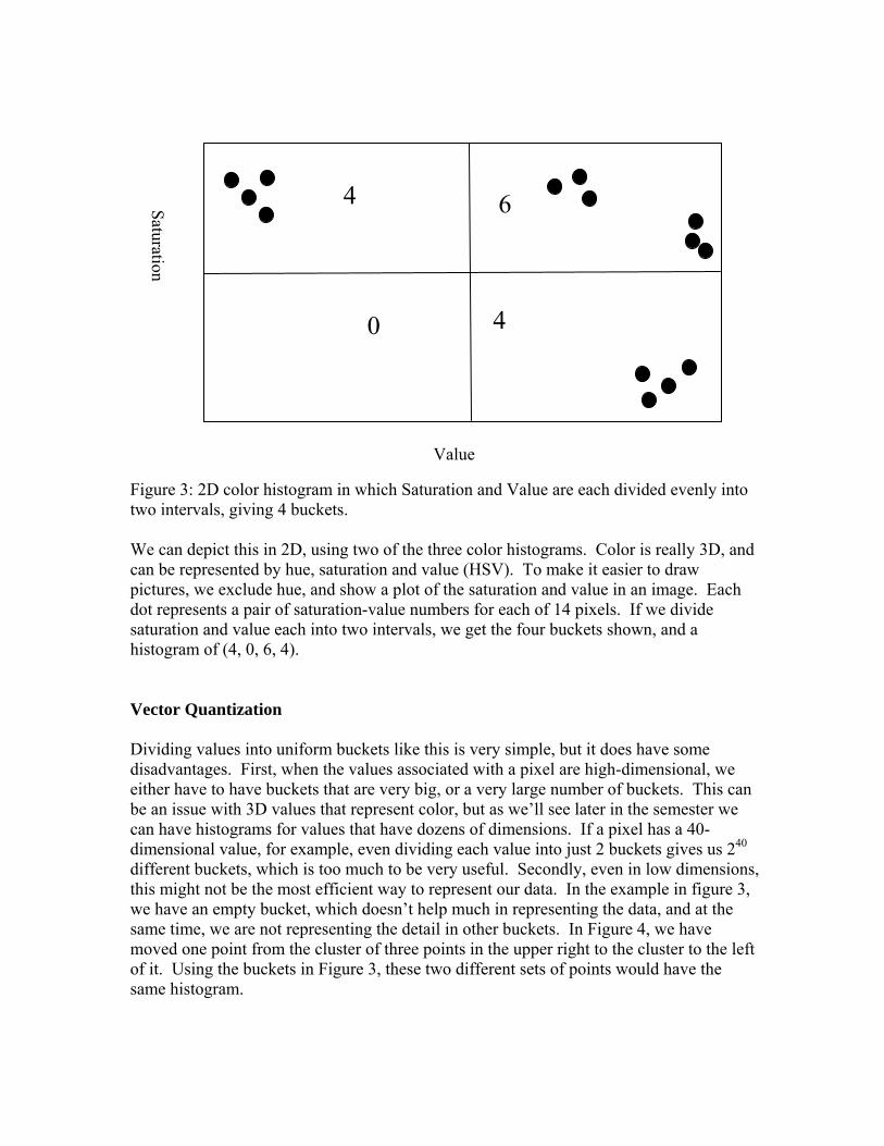
Figure 3: 2D color histogram in which Saturation and Value are each divided evenly into two intervals, giving 4 buckets. We can depict this in 2D, using two of the three color histograms. Color is really 3D, and can be represented by hue, saturation and value (HSV). To make it easier to draw pictures, we exclude hue, and show a plot of the saturation and value in an image. Each dot represents a pair of saturation-value numbers for each of 14 pixels. If we divide saturation and value each into two intervals, we get the four buckets shown, and a histogram of (4, 0, 6, 4). Vector Quantization Dividing values into uniform buckets like this is very simple, but it does have some disadvantages. First, when the values associated with a pixel are high-dimensional, we either have to have buckets that are very big, or a very large number of buckets. This can be an issue with 3D values that represent color, but as we’ll see later in the semester we can have histograms for values that have dozens of dimensions. If a pixel has a 40-dimensional value, for example, even dividing each value into just 2 buckets gives us 240 different buckets, which is too much to be very useful. Secondly, even in low dimensions, this might not be the most efficient way to represent our data. In the example in figure 3, we have an empty bucket, which doesn’t help much in representing the data, and at the same time, we are not representing the detail in other buckets. In Figure 4, we have moved one point from the cluster of three points in the upper right to the cluster to the left of it. Using the buckets in Figure 3, these two different sets of points would have the same histogram.

Value

Saturation

6 4

0 4

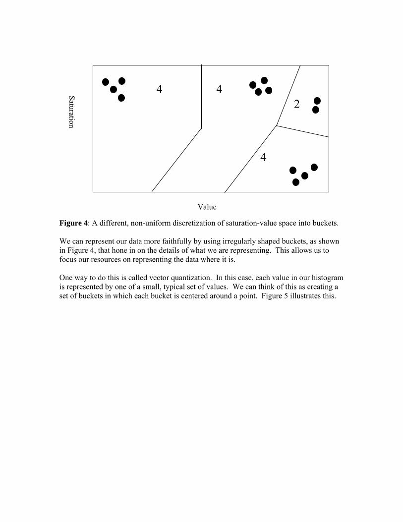
Figure 4: A different, non-uniform discretization of saturation-value space into buckets. We can represent our data more faithfully by using irregularly shaped buckets, as shown in Figure 4, that hone in on the details of what we are representing. This allows us to focus our resources on representing the data where it is. One way to do this is called vector quantization. In this case, each value in our histogram is represented by one of a small, typical set of values. We can think of this as creating a set of buckets in which each bucket is centered around a point. Figure 5 illustrates this.

Value

Saturation

2 4

4

4

Figure 5: Red points indicate the centers of buckets. Each black point is assigned to a bucket centered around the closest red point. Circles indicate which points belong to each bucket. More formally, suppose we have a set of points, p1,p2, …pn. And somehow we have found a set of bucket centers, q1, q2, …, qm. Point pi is assigned to bucket qj when: || pi-qj||<=|| pi-qk|| for all k≠j (here ||x|| represents the magnitude of x). We can build a histogram with m buckets by counting the number of points that belong to each bucket. To find out about one way of finding a good set of bucket centers, you can refer to the document on the K-means algorithm. The main idea is that we want to find the bucket centers that minimize the total distance from all points to their nearest bucket center. One application of this is color quantization. The simplest way to represent the color of a pixel in Matlab is to represent the red, green and blue values of each pixel with 8 bits, for a total of 24 bits per pixel. However, this is kind of wasteful, since it allows us to represent about 16 million different colors, when any one image can be depicted with many fewer colors. Suppose instead, we quantize our colors into 256 buckets, using the method described above (that is, we use m = 256). Then, each color in the image is replaced by the color of the nearest bucket center. To describe an image, for every pixel we only need to indicate which of the 256 buckets it belongs to, which takes just 8 bits, instead of 24. We also need to keep a list of the colors of the 256 bucket centers, but this is a small amount of data compared to the whole image. For example, if we have a megapixel image, we would use 3 megabytes to represent the colors in a simple way, but with color quantization we would only need 1 megabyte + 768 pixels. Of course, we lose some fidelity to the original image this way, since each color changes a little, but if we use enough cluster centers this is hardly noticeable. This is illustrated in Figure 6, using an image and code from Matlab (see rgb2ind. Better results can be obtained by also using dithering, as described in the help for that command).

Value

Saturation

Figure 6: In the upper left is a 24 bit color representation of an image of peppers. In the upper right, we quantize the colors to 256 values. The next row contains 128 and 64 color values, then 32 and 16, and finally an image with 4 different colors.

Still to come: Interpreting Histograms as Probability Distributions Smoothing Histograms