Class Averaging in Cryo-Electron Microscopy

Zhizhen Jane ZhaoCourant Institute of Mathematical Sciences, NYU

Mathematics in Data SciencesICERM, Brown University

July 30 2015

Single Particle Reconstruction (SPR) using cryo-EM

Challenges in Cryo-EM SPR

◮ Extremely low signal to noiseratio because of the lowelectron dose.

◮ Need to process a largenumber of images for desiredresolution.

◮ With higher resolutioncamera, the number of pixelsin each image becomes larger.

◮ Requires efficient andaccurate algorithms.

Geometry of the Projection Image

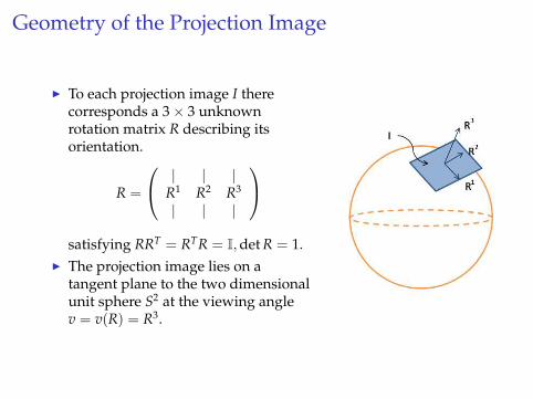
◮ To each projection image I therecorresponds a 3 × 3 unknownrotation matrix R describing itsorientation.

R =

| | |R1 R2 R3

| | |

satisfying RRT = RTR = I,det R = 1.

◮ The projection image lies on atangent plane to the two dimensionalunit sphere S2 at the viewing anglev = v(R) = R3.

Algorithmic Procedure for SPR

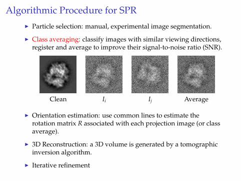
◮ Particle selection: manual, experimental image segmentation.

◮ Class averaging: classify images with similar viewing directions,register and average to improve their signal-to-noise ratio (SNR).

Clean Ii Ij Average

◮ Orientation estimation: use common lines to estimate therotation matrix R associated with each projection image (or classaverage).

◮ 3D Reconstruction: a 3D volume is generated by a tomographicinversion algorithm.

◮ Iterative refinement

Clustering Method (Penczek, Zhu, Frank 1996)

◮ Suppose we have n images I1, . . . , In.

◮ Rotationally Invariant Distances (RID) for each pair of images is

dRID(i, j) = minα∈[0,2π)

‖Ii − Rα(Ij)‖.

◮ Cluster the images using K-means.

◮ Problems:

1. Computationally expensive to compute all pairs of dRID. Naıveimplementation requires O(n2) rotational alignment of images.Rotational invariant image representation, fast algorithms fordimensionality reduction and nearest neighbor search.

2. Noise and outliers: At low SNR images with completely differentviews have relatively small dRID (noise aligns well, instead ofunderlying signal).Fast steerable PCA, Wiener filtering, and vector diffusion maps.

Hairy Ball Theorem and Global Alignment

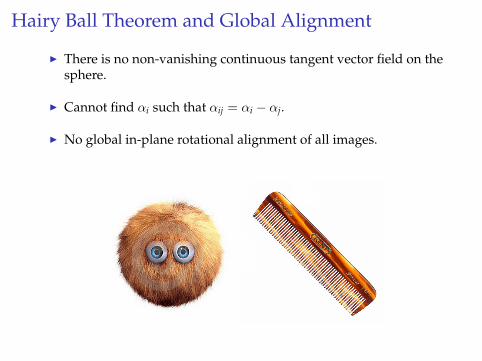
◮ There is no non-vanishing continuous tangent vector field on thesphere.

◮ Cannot find αi such that αij = αi − αj.

◮ No global in-plane rotational alignment of all images.

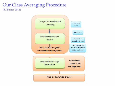
Our Class Averaging Procedure(Z., Singer 2014)

Comparison with Existing Methods

104 simulated projection images of 70S ribosome at different signal tonoise ratio. 50 nearest neighbors. Proportion of the nearest neighborswithin a small spherical cap of 18.2◦.

RFA/K-means IMAGIC Relion EMAN2 Xmipp ASPIRE

SNR= 1/50 0.45 0.97 0.79 0.74 0.83 1.00

SNR= 1/100 0.09 0.87 0.70 0.45 0.68 0.99

SNR= 1/150 0.07 0.67 0.52 0.13 0.48 0.90

Timing (hrs) 1.5 7.5 16 12 42 0.5

(a) IMAGIC (b) Relion (c) EMAN2 (d) Xmipp (e) ASPIRE (f) Reference

Ab initio Reconstruction of Experimental Data Sets

40, 778 images of 70S ribosome (Courtesy Dr Joachim Frank)Image size: 250 × 250 pixels. Pixel size: 1.5 A

*******************************************Movie of 70S ribosome

*******************************************

Ab initio model resolution: 11.5A.

Rotational Invariant Representation: Bispectrum

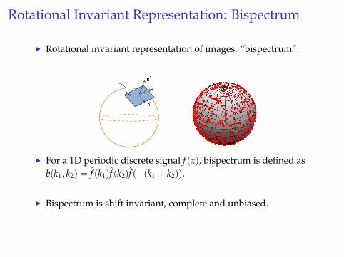
◮ Rotational invariant representation of images: “bispectrum”.

◮ For a 1D periodic discrete signal f (x), bispectrum is defined as

b(k1, k2) = f (k1)f (k2)f (−(k1 + k2)).

◮ Bispectrum is shift invariant, complete and unbiased.

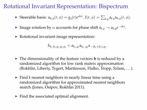
Rotational Invariant Representation: Bispectrum

◮ Steerable basis: uk,q(r, φ) = gq(r)eıkφ. I(r, φ) =

∑k,q ak,quk,q(r, φ).

◮ Image rotation by α accounts for phase shift ak,q → ak,qe−ıkα.

◮ Rotational invariant image representation:

bk1,k2,q1,q2,q3= ak1,q1

ak2,,q2a−(k1+k2),q3

.

◮ The dimensionality of the feature vectors b is reduced by arandomized algorithm for low rank matrix approximation(Rokhlin, Liberty, Tygert, Martinsson, Halko, Tropp, Szlam, . . . ).

◮ Find k nearest neighbors in nearly linear time using arandomized algorithm for approximated nearest neighborssearch (Jones, Osipov, Rokhlin 2011).

◮ Find the associated optimal alignment.

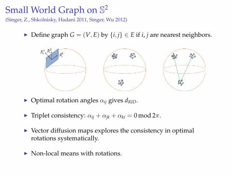
Small World Graph on S2

(Singer, Z., Shkolnisky, Hadani 2011, Singer, Wu 2012)

◮ Define graph G = (V,E) by {i, j} ∈ E if i, j are nearest neighbors.

◮ Optimal rotation angles αij gives dRID.

◮ Triplet consistency: αij + αjk + αki = 0 mod 2π.

◮ Vector diffusion maps explores the consistency in optimalrotations systematically.

◮ Non-local means with rotations.

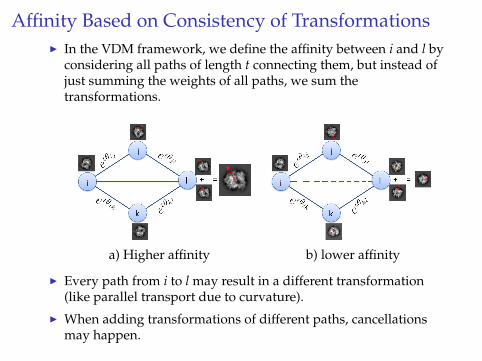
Affinity Based on Consistency of Transformations

◮ In the VDM framework, we define the affinity between i and l byconsidering all paths of length t connecting them, but instead ofjust summing the weights of all paths, we sum thetransformations.

a) Higher affinity b) lower affinity

◮ Every path from i to l may result in a different transformation(like parallel transport due to curvature).

◮ When adding transformations of different paths, cancellationsmay happen.

Initial vs VDM Classification

Noisy (SNR = 1/50) centered 104 simulated projection images of 70Sribosome. k = 200

0 60 120 1800

1

2

3

4

5

6x 10

5

acos〈vi, vj〉

N

0 5 10 15 20 25 300

2

4

6

8

10x 10

4

acos〈vi, vj〉N

Initial Classification VDM

Steerable PCA(Z., Singer 2013, Z., Shkolnisky, Singer 2015)

◮ Inclusion of the rotated and reflected images for PCA in somecases is advantageous.

◮ Many efficient algorithms transform images onto polar grid.However, non-unitary transformation from Cartesian to polargrid changes the noise statistics.

◮ A digital image I is obtained by sampling a squared-integrablebandlimited function f on a Cartesian grid of size L × L withbandlimit c. The underlying clean image is essentially compactlysupported in a disk of radius R.

◮ Suppose we have n images, we introduce an algorithm withcomputational complexity O(nL3 + L4) (O(nL4 + L6) for PCA).

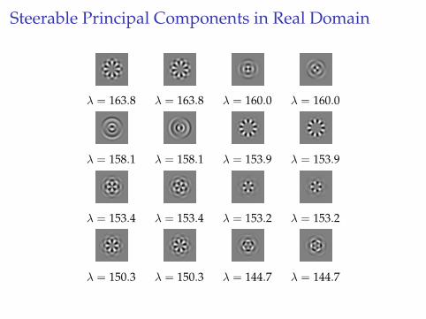
Steerable Principal Components in Real Domain

λ = 163.8 λ = 163.8 λ = 160.0 λ = 160.0

λ = 158.1 λ = 158.1 λ = 153.9 λ = 153.9

λ = 153.4 λ = 153.4 λ = 153.2 λ = 153.2

λ = 150.3 λ = 150.3 λ = 144.7 λ = 144.7

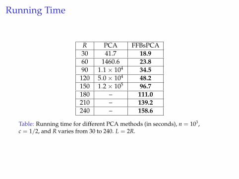
Running Time

R PCA FFBsPCA30 41.7 18.9

60 1460.6 23.8

90 1.1 × 104 34.5

120 5.0 × 104 48.2

150 1.2 × 105 96.7

180 – 111.0

210 – 139.2

240 – 158.6

Table: Running time for different PCA methods (in seconds), n = 103,c = 1/2, and R varies from 30 to 240. L = 2R.

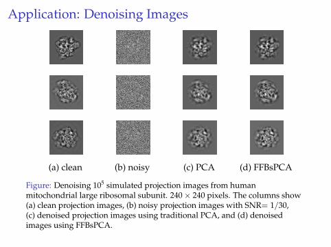
Application: Denoising Images

(a) clean (b) noisy (c) PCA (d) FFBsPCA

Figure: Denoising 105 simulated projection images from humanmitochondrial large ribosomal subunit. 240 × 240 pixels. The columns show(a) clean projection images, (b) noisy projection images with SNR= 1/30,(c) denoised projection images using traditional PCA, and (d) denoisedimages using FFBsPCA.

Outline of the Approach

◮ Truncated Fourier-Bessel expansion by a sampling criterion(asymptotics of Bessel functions).

◮ Efficient and accurate evaluation of the expansion coefficients(NUFFT and a Gaussian quadrature rule).

◮ Averaging over all rotations gives block diagonal structure in thesample covariance matrix and reduces computationalcomplexity.

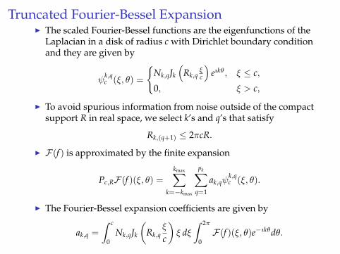
Truncated Fourier-Bessel Expansion◮ The scaled Fourier-Bessel functions are the eigenfunctions of the

Laplacian in a disk of radius c with Dirichlet boundary conditionand they are given by

ψk,qc (ξ, θ) =

{Nk,qJk

(Rk,q

ξc

)eıkθ, ξ ≤ c,

0, ξ > c,

◮ To avoid spurious information from noise outside of the compactsupport R in real space, we select k’s and q’s that satisfy

Rk,(q+1) ≤ 2πcR.

◮ F(f ) is approximated by the finite expansion

Pc,RF(f )(ξ, θ) =

kmax∑

k=−kmax

pk∑

q=1

ak,qψk,qc (ξ, θ).

◮ The Fourier-Bessel expansion coefficients are given by

ak,q =

∫ c

0

Nk,qJk

(Rk,q

ξ

c

)ξ dξ

∫ 2π

0

F(f )(ξ, θ)e−ıkθdθ.

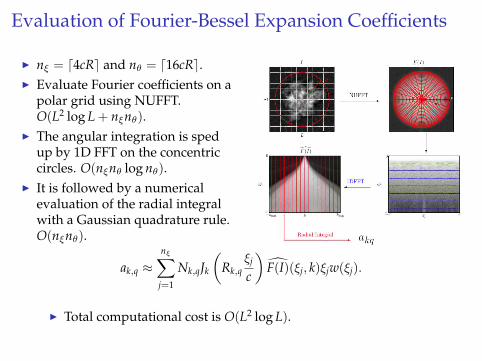
Evaluation of Fourier-Bessel Expansion Coefficients

◮ nξ = ⌈4cR⌉ and nθ = ⌈16cR⌉.

◮ Evaluate Fourier coefficients on apolar grid using NUFFT.O(L2 log L + nξnθ).

◮ The angular integration is spedup by 1D FFT on the concentriccircles. O(nξnθ log nθ).

◮ It is followed by a numericalevaluation of the radial integralwith a Gaussian quadrature rule.O(nξnθ).

ak,q ≈nξ∑

j=1

Nk,qJk

(Rk,q

ξj

c

)F(I)(ξj, k)ξjw(ξj).

◮ Total computational cost is O(L2 log L).

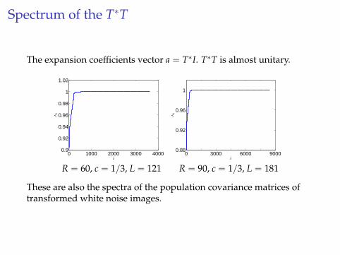
Spectrum of the T∗T

The expansion coefficients vector a = T∗I. T∗T is almost unitary.

0 1000 2000 3000 40000.9

0.92

0.94

0.96

0.98

1

1.02

i

λi

0 3000 6000 90000.88

0.92

0.96

1

i

λi

R = 60, c = 1/3, L = 121 R = 90, c = 1/3, L = 181

These are also the spectra of the population covariance matrices oftransformed white noise images.

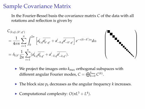
Sample Covariance Matrix

In the Fourier-Bessel basis the covariance matrix C of the data with allrotations and reflection is given by

C(k,q),(k′,q′)

=1

4πn

n∑

i=1

∫ 2π

0

[ai

k,qaik′,q′ + ai

−k,qai−k′,q′

]e−ı(k−k′)αdα

= δk,k′1

2n

n∑

i=1

(aik,qai

k,q′ + ai−k,qai

−k,q′).

◮ We project the images onto kmax orthogonal subspaces with

different angular Fourier modes, C =⊕kmax

k=0 C(k).

◮ The block size pk decreases as the angular frequency k increases.

◮ Computational complexity: O(nL3 + L4).

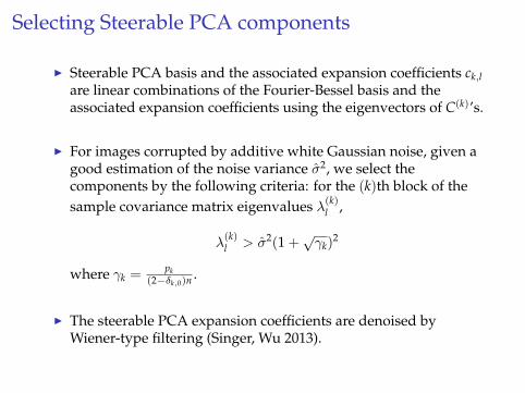
Selecting Steerable PCA components

◮ Steerable PCA basis and the associated expansion coefficients ck,l

are linear combinations of the Fourier-Bessel basis and theassociated expansion coefficients using the eigenvectors of C(k)’s.

◮ For images corrupted by additive white Gaussian noise, given agood estimation of the noise variance σ2, we select thecomponents by the following criteria: for the (k)th block of the

sample covariance matrix eigenvalues λ(k)l ,

λ(k)l > σ2(1 +

√γk)

2

where γk =pk

(2−δk,0)n .

◮ The steerable PCA expansion coefficients are denoised byWiener-type filtering (Singer, Wu 2013).

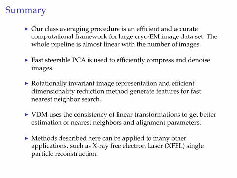
Summary

◮ Our class averaging procedure is an efficient and accuratecomputational framework for large cryo-EM image data set. Thewhole pipeline is almost linear with the number of images.

◮ Fast steerable PCA is used to efficiently compress and denoiseimages.

◮ Rotationally invariant image representation and efficientdimensionality reduction method generate features for fastnearest neighbor search.

◮ VDM uses the consistency of linear transformations to get betterestimation of nearest neighbors and alignment parameters.

◮ Methods described here can be applied to many otherapplications, such as X-ray free electron Laser (XFEL) singleparticle reconstruction.

References

◮ Z. Zhao, Y. Shkolnisky, A. Singer, “Fast Steerable PrincipalComponent Analysis”, Submitted, Available athttp://arxiv.org/abs/1412.0781.

◮ Z. Zhao, A. Singer, “Rotationally Invariant Image Representationfor Viewing Direction Classification in Cryo-EM”, Journal ofStructural Biology, 186 (1), pp. 153-166 (2014).

◮ Z. Zhao, A. Singer, “Fourier-Bessel Rotational InvariantEigenimages”, The Journal of the Optical Society of America A, 30

(5), pp. 871-877 (2013).

◮ A. Singer, H.-T. Wu, “Vector Diffusion Maps and the ConnectionLaplacian”, Communications on Pure and Applied Mathematics, 65

(8), pp. 1067-1144 (2012).

◮ A. Singer, Z. Zhao, Y. Shkolnisky, R. Hadani, “Viewing AngleClassification of Cryo-Electron Microscopy Images usingEigenvectors”, SIAM Journal on Imaging Sciences, 4 (2), pp.723-759 (2011).

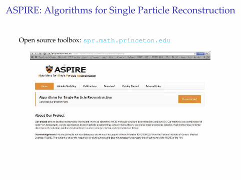
ASPIRE: Algorithms for Single Particle Reconstruction

Open source toolbox: spr.math.princeton.edu

Thank You!